
Factors Influencing the Accuracy of Shallow Snow Depth Measured Using UAV-Based Photogrammetry


Department of Civil and Environmental Engineering, Hongik University, Seoul 04066, Korea
*
Author to whom correspondence should be addressed.
Remote Sens. 2021, 13(4), 828; https://0-doi-org.brum.beds.ac.uk/10.3390/rs13040828
Submission received: 27 January 2021
/
Revised: 18 February 2021
/
Accepted: 19 February 2021
/
Published: 23 February 2021
(This article belongs to the Special Issue Measurement of Hydrologic Variables with Remote Sensing)
Abstract
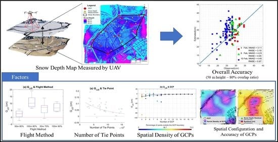
:Factors influencing the accuracy of UAV-photogrammetry-based snow depth distribution maps were investigated. First, UAV-based surveys were performed on the 0.04 km2 snow-covered study site in South Korea for 37 times over the period of 13 days under 16 prescribed conditions composed of various photographing times, flight altitudes, and photograph overlap ratios. Then, multi-temporal Digital Surface Models (DSMs) of the study area covered with shallow snow were obtained using digital photogrammetric techniques. Next, the multi-temporal snow depth distribution maps were created by subtracting the snow-free DSM from the multi-temporal DSMs of the study area. Then, snow depth in these UAV-Photogrammetry-based snow maps were compared to the in situ measurements at 21 locations. The accuracy of each of the multi-temporal snow maps were quantified in terms of bias (median of residuals, ) and precision (the Normalized Median Absolute Deviation, NMAD). Lastly, various factors influencing these performance metrics were investigated. The results are as follows: (1) the and NMAD of the eight surveys performed at the optimal condition (50 m flight altitude and 80% overlap ratio) ranged from −2.30 cm to 5.90 cm and from 1.78 cm to 4.89 cm, respectively. The best survey case had −2.30 cm of and 1.78 cm of NMAD; (2) Lower UAV flight altitude and greater photograph overlap lower the NMAD and ; (3) Greater number of Ground Control Points (GCPs) lowers the NMAD and ; (4) Spatial configuration and accuracy of GCP coordinates influenced the accuracy of the snow depth distribution map; (5) Greater number of tie-points leads to higher accuracy; (6) Smooth fresh snow cover did not provide many tie-points, either resulting in a significant error or making the entire photogrammetry process impossible.
1. Introduction
Snowfall in most regions of Korea occurs in the form of shallow snow, a term referring to snow with depth of less than 20 cm. Shallow snowpacks pose significant impacts on ecosystems. For example, shallow snowpacks increase surface albedo, causing the depth of frozen soil to increase [1]. This subsequently leads to greater erosion of soil [2], which contains high concentration of phosphorous and nitrogen, playing important role in plant growth [3,4]. Shallow snowpacks also influence animal habitat and predation by altering food availability [5,6,7]. Therefore, to study and model the behavior of shallow snowpacks, it is important to first measure them precisely.
However, it is difficult to measure shallow snowpacks precisely because of their high spatio-temporal variability [8,9,10]. While efforts have been made to estimate the spatial variability of shallow snow depths [11,12,13], most publicly available snow depth data are provided in the format of a set of sparsely placed point measurements or of low-resolution raster data [14] that are not accurate and precise enough to be used as input for hydrological models aimed at estimating snowmelts, groundwater recharge, and soil erosion.
Remote sensing technology have been actively applied to estimate the accumulated snow depth and spatial extent. Microwave sensors [15,16,17,18] and optical sensors [19,20,21,22,23,24] on-board satellites or the combination of both [25,26,27,28] have been used. In addition, on-board aircraft sensors have been used [29,30].
Unmanned Aerial Vehicles (UAVs), which recently went through dramatic technological advancement, emerged as the spotlight of the field of surveying in the last decades. Accordingly, snow depth surveying utilizing UAV was also a part of the spotlight [31]. The techniques of photogrammetry [32,33] can construct three-dimensional models of snow fields from multiple photographs taken from UAV, so it has been recently applied to estimate the snow depth [34,35,36]. Table 1 summarizes the results of studies that estimated snow depths using UAV-photogrammetry.
This study also applied the UAV-photogrammetry method to estimate the snow depth, but is distinctive from the studies summarized in the Table 1 as follows: (1) The lowest NMAD validated based on 21 in situ measurements is 1.78 cm, which is significantly lower than other previous studies; (2) This study analyzed how the accuracy of the estimated snow depth varies with regard to varying conditions of photography, such as altitude, photograph overlap ratio, time of survey, and condition of GCPs.
2. Methodology
2.1. Study Area
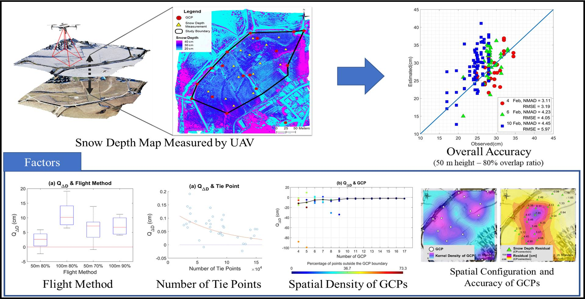
Figure 1 shows the study area, a small land patch located in Daegwallyeong-Myeon Pyoungchang-Gun Kangwon-Do of South Korea (37.6860°N, 128.7416°E). This area has the highest average annual snowfall in Korea, of approximately 260 cm, and the three highest snow accumulation measurements recorded at the Daegwallyeong AWS station, 2 km away from the study site, are 189 cm (1989), 149 cm (2003), and 126 cm (2005). The study site has the approximate spatial dimension of 350 m (E-W) × 400 m (N-S). Figure 2 shows the accumulated snow depth measured by laser snow depth gauge at the Daegwallyeong AWS station during the surveying period. There were three snow events between 26 January and 30 January 2020, and the maximum accumulated snow depth was approximately 31 cm (recorded on 30 January 2020).
2.2. Survey Instrument Specification (UAV and GNSS Receiver)
A Phantom 4 Pro 2.0 (produced by DJI) was used to take the base photographs of this study. The drone has the maximum and recommended flight time of 30 min and 15 min, respectively. The maximum allowable wind velocity is 10 m/s [45]. It has the GPS/GLONASS positioning system and the hovering accuracy is ±0.1 m (vertical) and ±0.3 m (horizontal). The camera onboard the drone (DJI FC6310) has an image dimension of 5472 × 3648, a sensor size of 13.2 mm (width) × 8.8 mm (height), and a focal length of 8.8 mm. Each of the photographs are recorded with the positioning metadata, which contains the axis roll, pitch, and yaw of the camera along with the three-dimensional coordinate of the drone.
A Trimble R10 GNSS (Global Navigation Satellite System) receiver was used to measure the three-dimensional coordinates of the GCPs and the locations of in situ snow depth measurement [46]. The instrument uses the technology of Real-Time Kinematic (RTK), Virtual Reference Station Networks (VRSN), and Real Time eXtended (RTX) to secure the measurement precision. The maximum precision is 8 mm (horizontal) and 15 mm (vertical).
2.3. Acquisition of the Snow Depth Map
Process of the snow depth map acquisition comprises: (1) placing GCPs to secure the accuracy of the survey; (2) UAV photographing and photogrammetry to obtain the DSM of accumulated snow; and (3) UAV photographing and the photogrammetry to obtain DSM of the ground surface after snow completely melted. The map of the accumulated snow was obtained by subtracting the product of process (3) from that of process (2).
2.3.1. GCPs
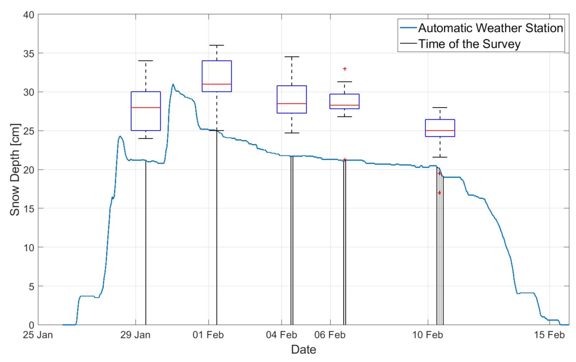
Before the snow events, 17 GCPs were chosen, where the coordinates (longitude, latitude, and height) were precisely measured using the GNSS receiver. These GCPs were chosen as the locations with easily identifiable landmarks, such as manholes on roads (Figure 3a,b). Snow on these locations was removed soon after the snow events, either by a researcher or by snow plowing vehicles operated by the local disaster management authority. Furthermore, we installed additional GCPs between the UAV surveying. A black planar object sized 50 cm × 50 cm was placed on the accumulated snow immediately prior to a set of UAV surveying (Figure 3c). Coordinates of an edge of the black planer object were measured using the GNSS receiver precisely considering the vertical location of the sensor in the instrument and the manually measured snow depth (Figure 3c). The green circles in Figure 1c show the location of the 17 GCPs used by this study.
Figure 4 shows the box plot of the horizontal and vertical uncertainties calculated for each of the surveying days. Each box plot was drawn based on the coordinates of 17 GCPs. All horizontal and vertical uncertainties ranged under 1.6 cm and 2.8 cm, suggesting that the in situ GCP positioning was successful.
2.3.2. UAV Surveying Campaigns
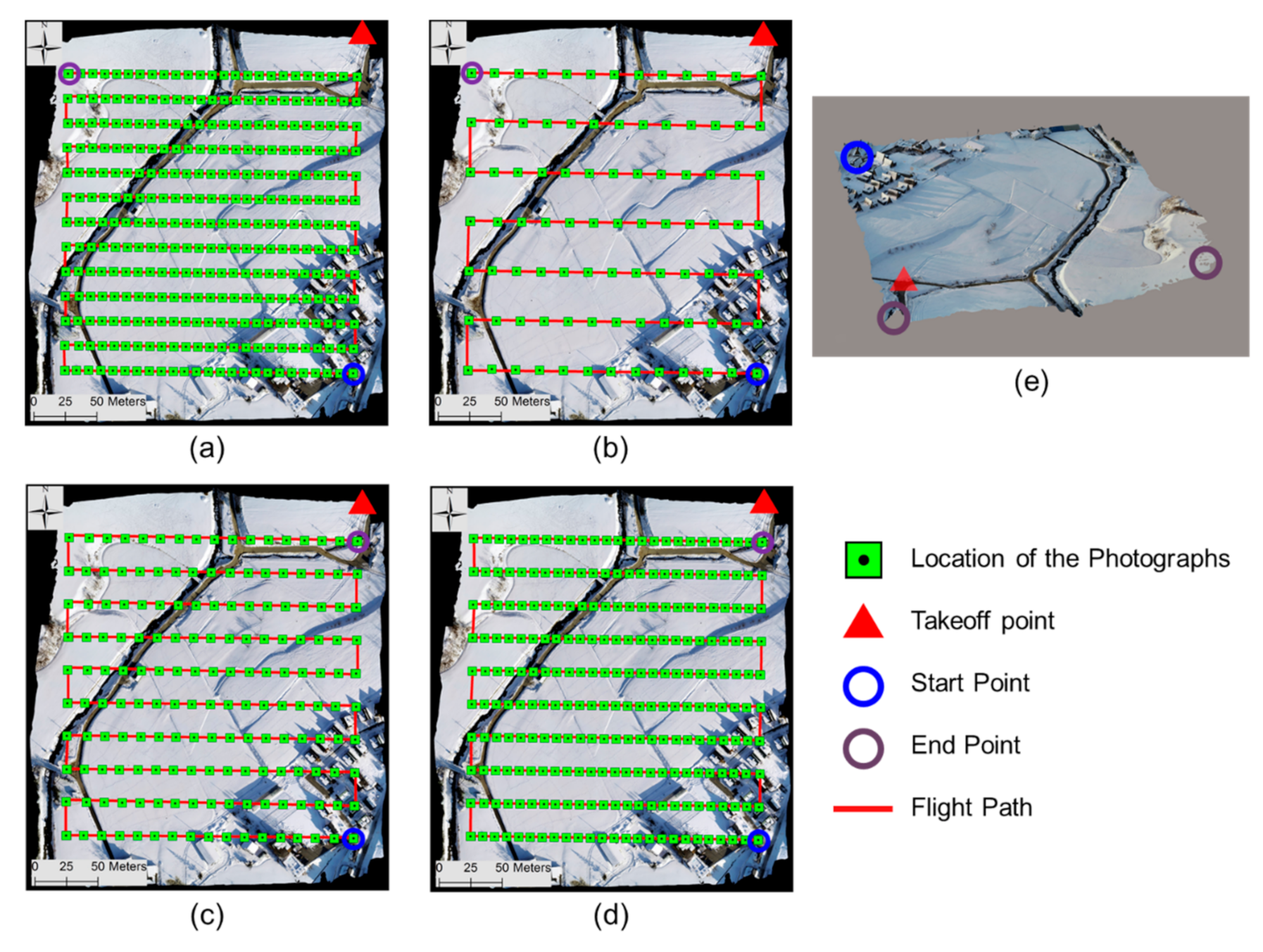
The UAV surveying campaigns were repeated 37 times after and between the three snow events with varying conditions of UAV altitude, photograph overlap ratio, and surveying time of day, as summarized in Table 2 and Table 3. Figure 5a–d shows the flight path and shooting locations with different overlap ratios and flight altitudes. Figure 5e shows the DSM of the study area viewed from the UAV take-off position.
2.3.3. Photogrammetric Processing to Obtain the DSM
Photographs taken from the UAV were fed into the photogrammetry software tool, ContextCapture, Bentley [47], to produce the DSM and orthomosaic of the study site with accumulated snow. Here, we describe the general process of photogrammetry instead of the one actually employed by the software tool, which is kept confidential. The process is composed of the following three steps:
- Camera calibration: this is the process of estimating camera’s intrinsic parameters such as its focal length, skew, distortion, and image center. This is first done by identifying common features in multiple photographs of which real-world 3D coordinates are precisely known (such as GCPs). Then, a set of equations [48] are solved to obtain the camera intrinsic parameters. Here, some of the intrinsic parameters are precisely provided by the camera manufacturer (e.g., focal length) and can be directly adopted. The intrinsic parameters are used to correct the distortion of the photographs and they apply to all photographs, so the accurate 2D coordinates of the pixels in all photographs can be obtained in this step.
- Structure from Motion (SfM): in this process, the tie-points, which are another set of features that coexists in a series of photographs, are first identified. Then, an optimization process of which the objective function is composed of a set of collinearity equations [37,49,50] are solved to obtain extrinsic parameters of the camera (e.g., position and orientation of camera corresponding to all photographs) and 3D coordinates of the tie-points. Here, the key to successful implementation is the automated algorithms for tie-point detection, which requires the comparison between all input photographs [51].
- Bundle Adjustment: the GCPs, as opposed to tie-points, have the precisely known pair of 2D and 3D coordinates, which are also included in the objective function of the optimization process. Therefore, accuracy and the spatial configuration of GCPs greatly influences accuracy of photogrammetry.
- DSM construction. In this step, the triangular irregular network, which is composed of tie-points, is constructed and textures extracted from photographs are applied to obtain the DSM. Here, the accuracy of the DSMs may be estimated by performing the pixel-wise correlation analysis.
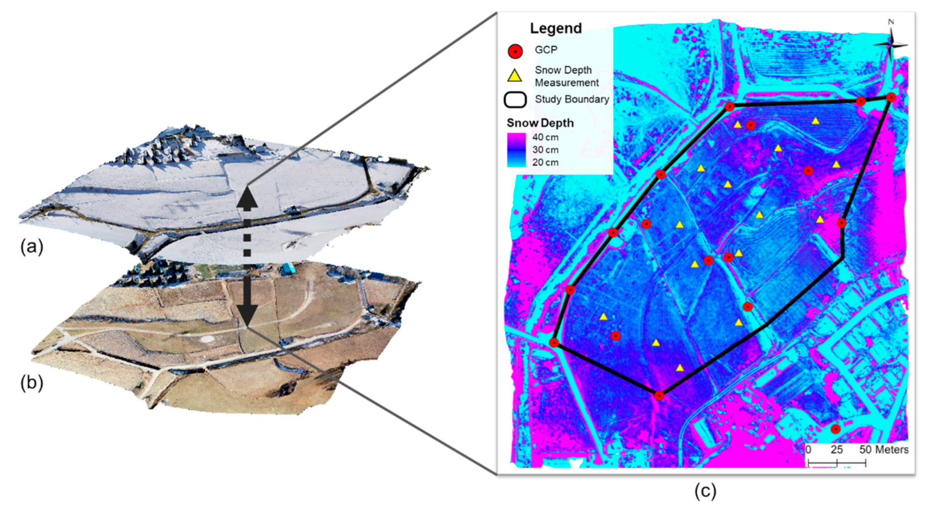
After the snow completely melted, a UAV survey was performed to obtain the DSM of the ground surface of the study site. A greater accuracy would have been achieved if the site was surveyed immediately before the snow event because the ground surfaces slightly deform as snow melts and runs off the ground. However, this was unfortunately impossible because the large snow events, as investigated in this study, are rare in Korea and only after this kind of large snow event occurs, the study area can be fixed. The photogrammetry was performed using the 17 GCPs, shown as yellow stars in Figure 1c. The accuracy of the DSM of the ground surface was validated at seven check points (CPs), shown as X marks in Figure 1c. The RMSE and the NMAD were 2.75 cm and 1.19 cm, respectively. Figure 6a–c show the DSM of the study site (a) with and (b) without accumulated snow, and (c) the snow depth map, respectively. Note that the local distortion of elevation tends to occur at the edge of the DSM (magenta area in Figure 6c). This is primarily because the edges are not photographed from as diverse angles as the internal area. Another reason may be the sparse placement of GCPs. The black line in Figure 6c delineates the study area where in situ measurement and analysis were performed. Most of this internal study area is not influenced by the local distortion of the DSM.
2.4. In Situ Snow Depth Measurment and Validation
Immediately after each of the UAV survey campaigns (Table 2), the snow depth was manually measured using a stainless metal ruler at and around the 21 specified locations shown as red triangles in Figure 1c. The in situ snow depths corresponding to each survey day are expressed as box plots in Figure 2. They ranged between 17.5 cm and 36 cm and were consistently greater than the measurement at the AWS stations, while the temporal trends coincide. This degree of discrepancy is not surprising considering the high spatial and temporal variability of rainfall in Korea [52,53]. The estimated snow depth values obtained from photogrammetry were validated based on these in situ snow depth measurements.
The mean of residuals (, Equation (2)), tandard deviation of error (, Equation (3)), and Root-Mean-Square-Error (RMSE, Equation (4)) are the typical metrics to measure the accuracy of the survey. Here, note that the term “accuracy” represents the general closeness of a measurement to the true value, which refers to both bias and precision. The term “bias” represents a measure of how far the expected value of the estimate is from the true value, and the term “precision” represents a measure of how similar the multiple estimates are to each other:
where and represent the observed in situ snow depth and the snow depth estimated from the UAV photogrammetry at the ith measurement location, respectively, and (Equation (1)) represents the measurement error. These statistics (Equations (2)–(4)) can be good accuracy measurement metrics only if the measurement errors (s) are normally distributed. In addition, the uncertainty analysis results based on these statistics may be highly sensitive to a few measurement outliers, which are hard to filter out due to the ambiguous standard for detection. In such cases, the median of residuals ( and Normalized Median Absolute Deviation (NMAD, Equation (5)) can be good alternatives to quantify the bias and the precision, which are less sensitive to outliers [39,54]:
Therefore, this study used all five statistics (, , RMSE, , and ) to quantify the bias and precision of snow depth estimation.
3. Results
3.1. Overall Accuracy of The Snow Depth Map
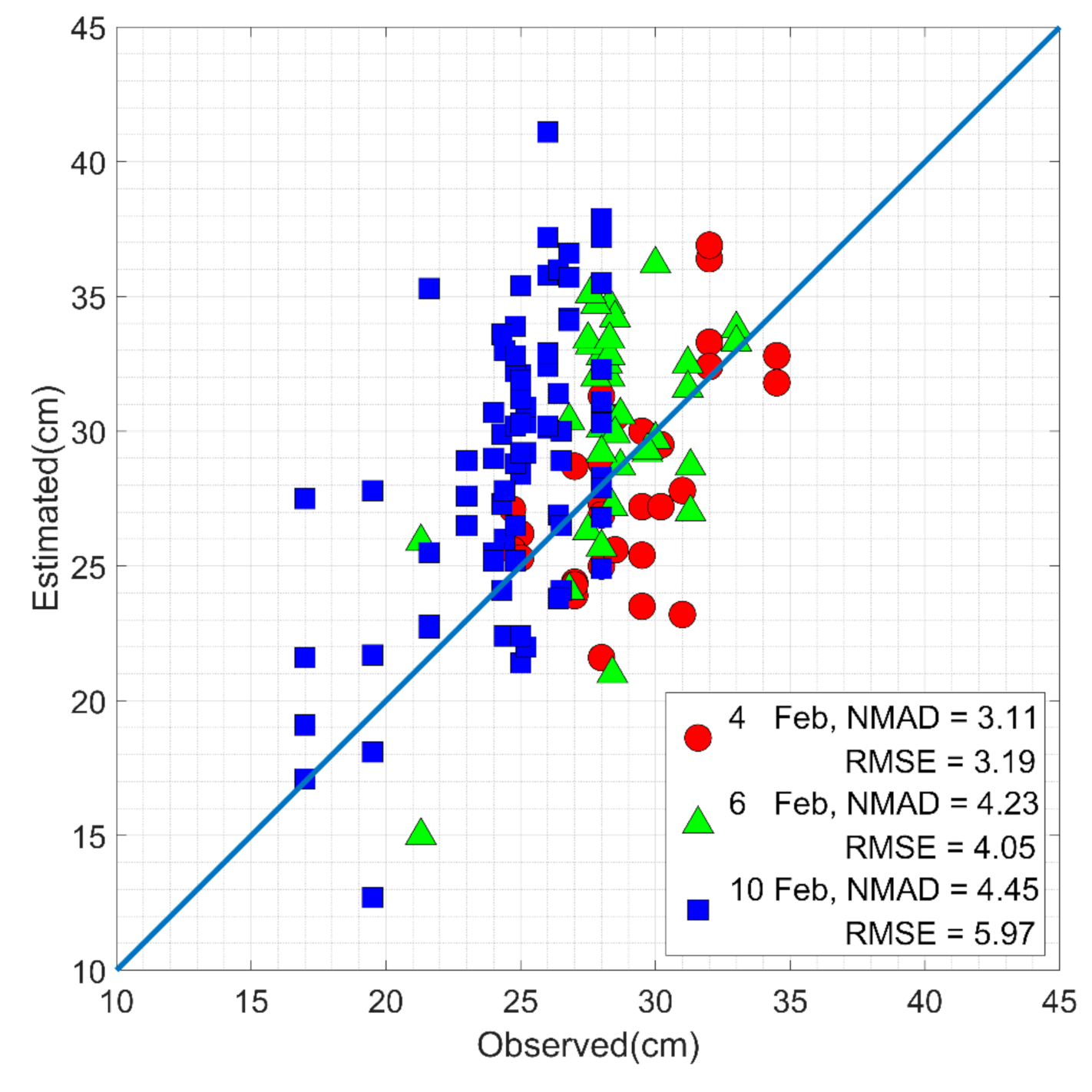
Figure 7 shows a scatter plot comparing the observed snow depth (x) and the snow depth estimated from the UAV photogrammetry (y) for the dates of 4th (red circles), 6th (green triangles), and 10 (blue squares) February. The results corresponding to 29 January and 1st February were not included because the photogrammetry process could not identify enough tie points due to the extremely smooth snow surface and the corresponding high reflectivity [35]. Thus, the snow map either could not be produced (29 January) or had very low accuracy (1 February). In addition, the results corresponding to 50 m of UAV altitude and 80 percent of photograph overlap are only shown here because this condition produced the lowest NMAD. The results corresponding to all four surveying times (9 a.m., 11 a.m., 1 p.m., and 3 p.m.) are shown in Table 4. The NMAD varied between 3.11 to 4.45 cm. The causes of varying accuracy are discussed in the later sections, because the residuals shown in Figure 7 were caused by a variety of factors, and thus, difficult to explain without isolating each of those factors. Note that the NMAD represents the precision of the measurement but not bias. The RMSE, which is the standard deviation of the residuals (), can be a good proxy for overall measurement accuracy reflecting both bias and precision. The RMSE varied between 3.19 cm and 5.97 cm. The causes of varying accuracy are discussed in the later sections, because the residuals shown in Figure 7 were caused by a variety of factors and are thus difficult to explain without isolating each of those factors.
3.2. Influence of the UAV Flight Altitude and the Photograph Overlap Ratio
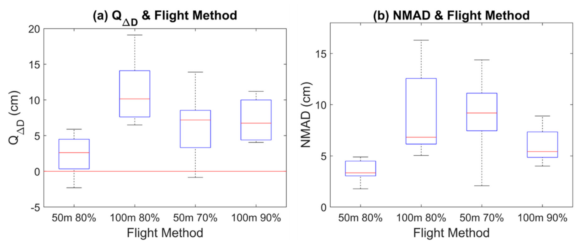
Figure 8 shows the box plots of the (a) and (b) NMAD of the estimated snow depth that varies with four different conditions of UAV flight altitudes and photograph overlap ratios. Low and NMAD is associated with low flight altitude and high photograph overlap. This is because a greater number of tie-points can be identified at low flight altitudes and high photograph overlap.
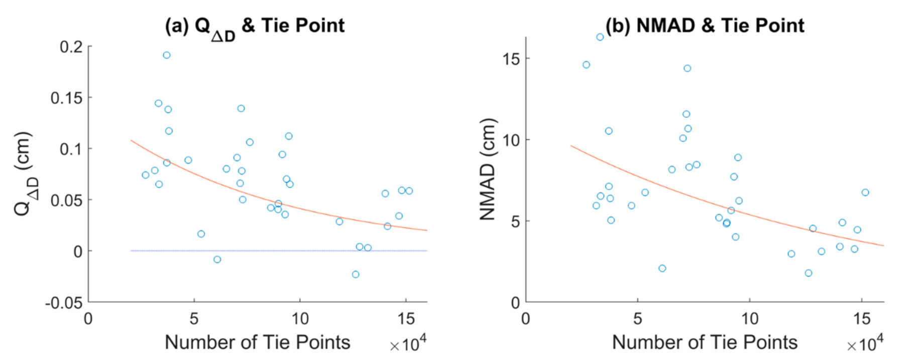
3.3. Influence of Number of Identified Tie-Points
Figure 9a,b shows the and the NMAD of each survey varying with the number of identified tie points. A greater number of tie points is associated with low and low NMAD of the estimated snow depth. The vertical variation in the scatters is associated with flight time, altitude, and overlap ratio, and the number, accuracy and spatial configuration of GCPs, which we explain in the following sections.
3.4. Influence of Spatial Density of GCPs
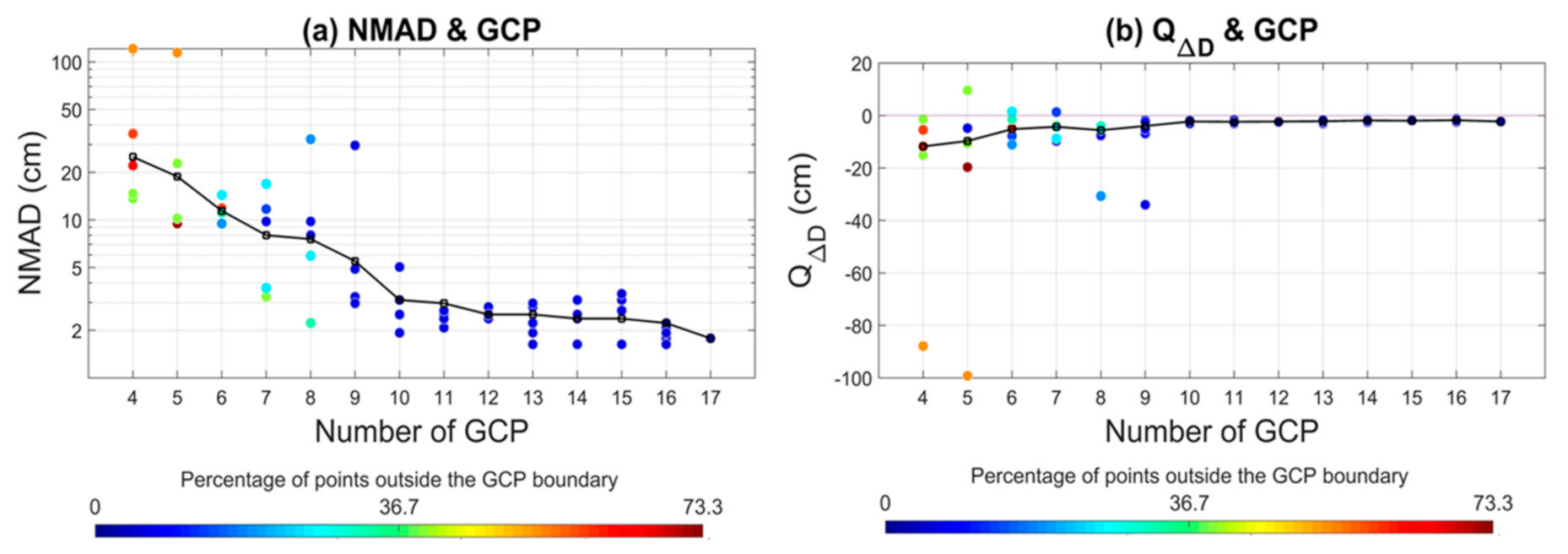
It is widely known that GCP spatial density affects the accuracy of photogrammetric surveys [55]. This study assumed that the same principle applies to the snow depth survey. To verify this hypothesis, this study repeated the process of intentionally removing the GCPs while performing the photogrammetric processing and recorded NMAD and of the estimated snow depth. Results with the lowest NMAD value (50 m height—80% overlap ratio, 4 February, 9 a.m.) were used for this experiment. Figure 10a,b show NMAD and of the estimated snow depth varying with the number of GCPs. The GCPs were removed evenly over the space so that the remaining GCPs are distributed equally over the space. The number of remaining GCPs varied between 4 and 17, which correspond to the spatial density of 0.4 GCP/km2 and 1.7 GCP/km2, respectively.
The magenta area of Figure 6c suggests sudden increases of snow depth, which strongly suggests that this area is associated with the error that is caused by the local deformation of DSM. This is a known issue of photogrammetry, which often happens at the area located outside the spatial networks of GCPs. This study performed an experiment to verify this assumption. The color of the points in Figure 10a,b represent the number of the in situ measurement locations outside the GCP network. The red points mean that most of the in situ measurement locations are located outside the GCP network, and vice versa. The vertical distribution of the color dots did not show a clear trend, which means that there are other important factors influencing the accuracy of the snow photogrammetry than the relative locations between the GCP network and in situ measurement locations. This suggests that the density and spatial distribution as well as type of GCP (i.e., road, manhole, and planar object on snow field) may be more critical factors influencing the accuracy of the snow photogrammetry. For example, most red colors were associated with the GCP network, containing many GCPs placed on snow field, which has relatively low accuracy. In addition, the GCPs were evenly placed over the study area, so no in situ measurement locations were truly further away from the GCP network, which may be another reason that the trend was not detected.
3.5. Influence of the Spatial Configuration and the Accuracy of the GCPs
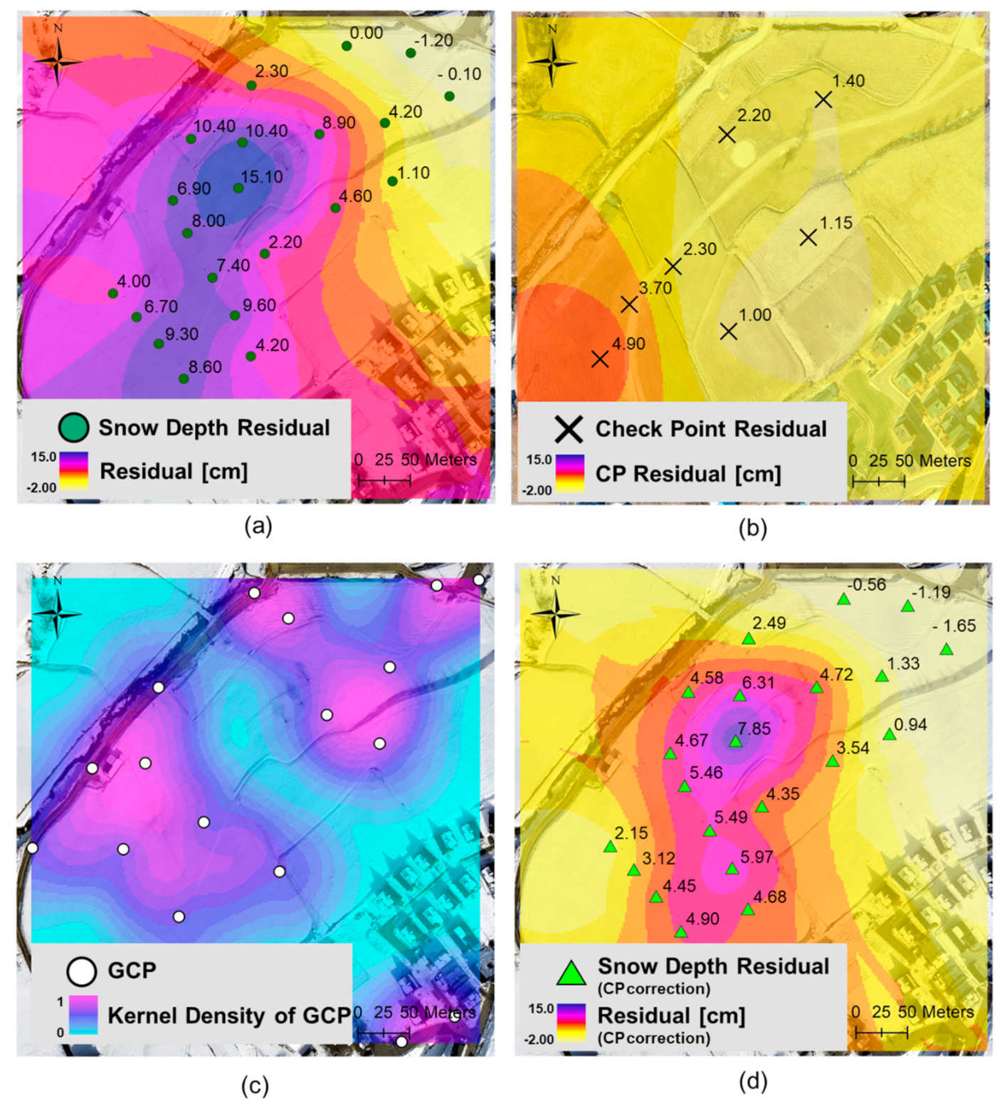
The spatial configuration as well as the spatial density of GCPs is important. Figure 11c shows the kernel density of spatially distributed GCP points; the pinker the area, the more GCPs are influencing the area. Figure 11a shows an interpolated map of snow depth residual of the estimated snow depth corresponding to the measurement with the overall lowest accuracy (50 m height—80% overlap ratio, 10 February, 3 p.m.). Figure 11b shows an interpolated map of CP residual of snow-free surface DSM, which were used to obtain Figure 11d, which is the map of the snow depth residual after CP correction. Figure 11c shows the kernel density of the GCPs. It is shown that the blue area of Figure 11c (area further away from GCPs) and the purple area of Figure 11d (area with greater estimation error) coincides, suggesting that the number of GCPs used for bundle adjustment may influence the accuracy of the photogrammetry.
4. Discussions
4.1. Influence of The Surveying Time
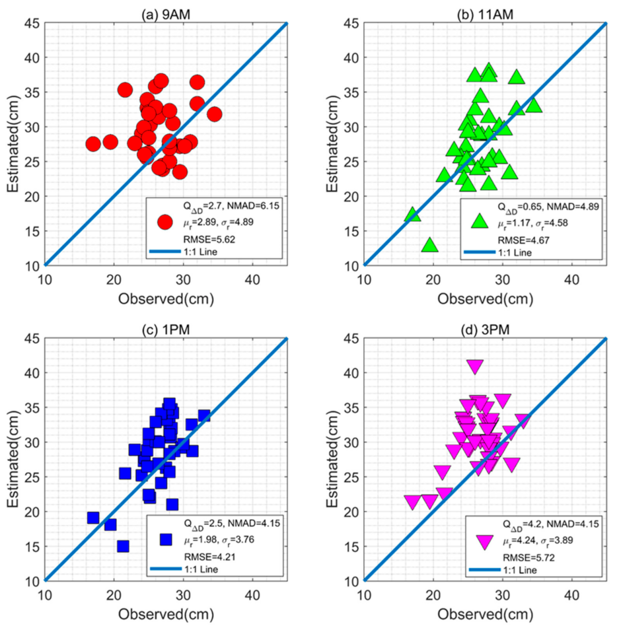
Figure 12 shows the scatter plot comparing the observed snow depth (x) and the snow depth estimated form the UAV photogrammetry (y) for the surveying time of (a) 9 a.m., (b) 11 a.m., (c) 1 p.m., and (d) 3 p.m., respectively. Results corresponding to the surveying condition of 50 m—80% for all dates (4, 6, and 10 February) are shown together in each scatter plot.
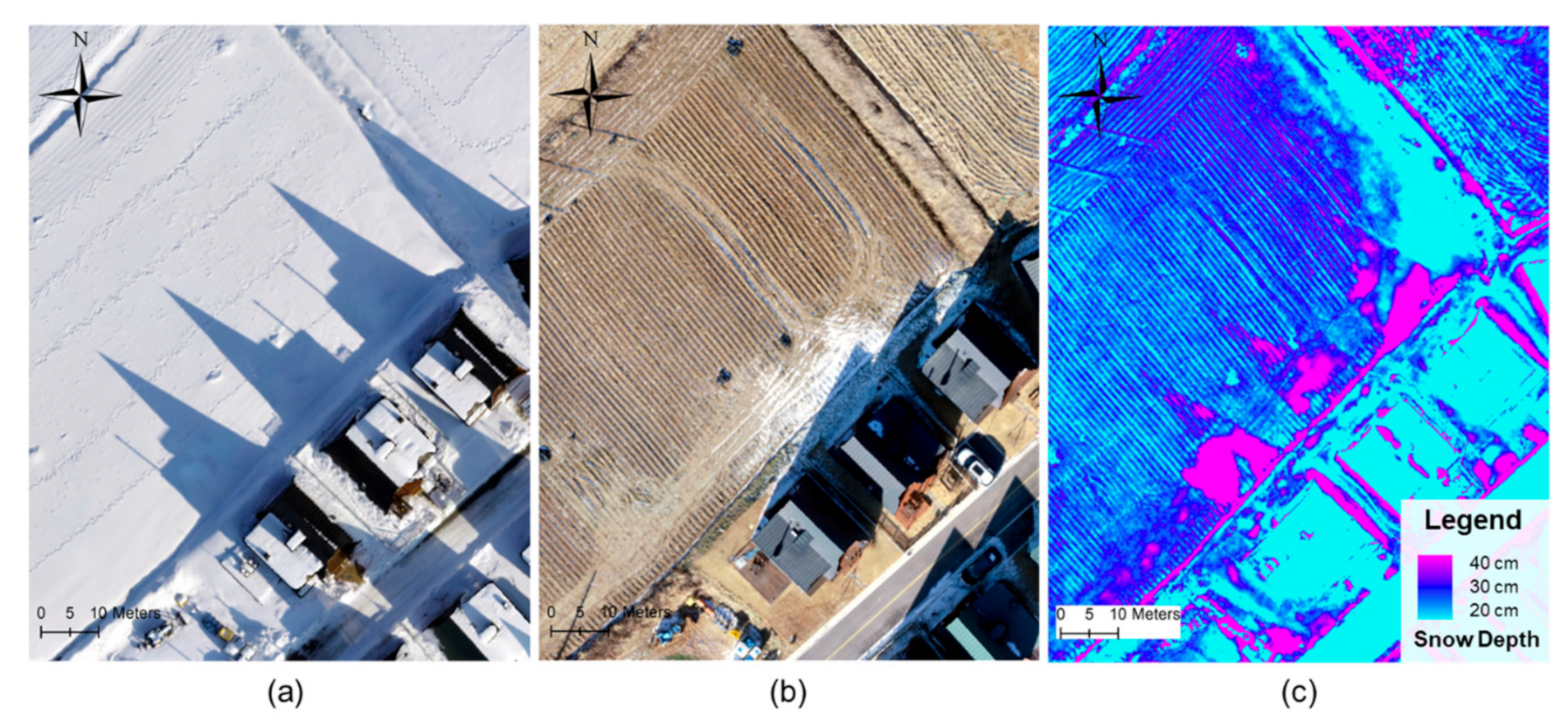
Significant positive bias is apparent for the surveying time of 9 a.m. and 3 p.m. One possible cause of this time-dependent accuracy is that shadows of the object generally degrade the accuracy of the photogrammetry result, and shadow sizes were greater as the surveying time was further away from noon. For example, the time lapse of the photographs existing between different swaths can be several minutes, and even in those several minutes, the size of the shadows can change significantly in early morning and late evening time [42]. In addition, clear contrast between snow and overlaying shadow induces significant positive bias in the photogrammetry result. Figure 13 shows the orthophoto and the estimated snow depth of a small fraction of the study site for 9 a.m. of 4 February. While the snow depth in the shadow seems not much different from the non-shaded area according to the orthophoto as shown in Figure 13a, the snow depth is significantly greater in the shadow area according to the photogrammetry, as shown in Figure 13c. These areas with high brightness contrast are greater for morning and evening time, which causes greater bias for the overall photogrammetry results.
4.2. Issues with Image Saturation
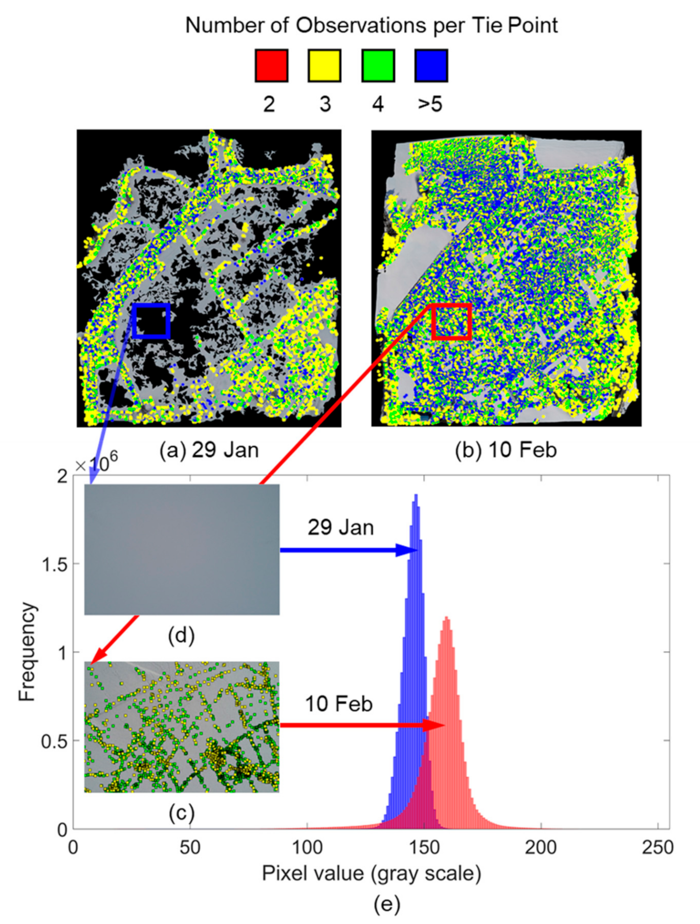
Figure 14a,b show the identified tie points and the orthophoto images (gray) during the survey of 29 January and 10 February, respectively. Figure 14c,d are the magnified view of the same subset of the images. Color of the points represents the number of photos that identified corresponding pixel location as a tie point. Inspection of survey data for 29 January shows that not as many tie points could be identified as were identified from data for 10 February, because the snow field initially had a very smooth surface on 29 January. Then, wind and uneven melting caused rifts on the field, dramatically increasing the number of tie points for the survey of 10 February.
The histograms (Figure 14e) of the orthomosaic subsets (Figure 14c,d) reveal that the colors of 26 January photographs are limited to within a very narrow range of the colors, while the colors of 10 February photographs are significantly more diverse.
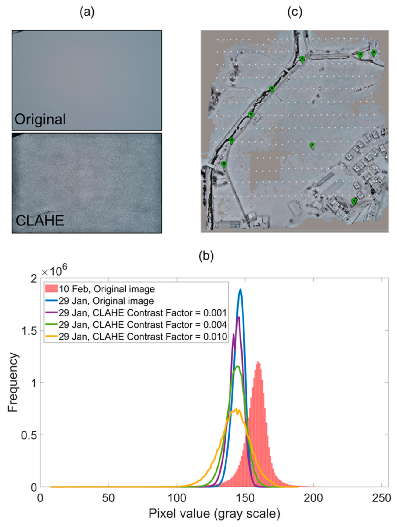
This issue of image oversaturation as shown through the case of the 29 January may be resolved through the application of the Contrast Limited Adaptive Histogram Equalization (CLAHE) technique. Figure 15a compares the same subset of the area (shown as Figure 14a) before and after applying the CLAHE filter. The comparison shows that the filter significantly resolves the issue of image saturation. Following this finding, we performed an experiment to see if the different levels of contrast factor of CLAHE filter increases the number of tie points. Figure 15b shows the grayscale histograms of the image of the entire study area corresponding to the contrast factor (CF) of 0 (no filter), 0.001, 0.004, and 0.010, respectively. The number of the identified tie points corresponding to each filter was 30,310 (no filter), 32,789 (CF = 0.001), 33,495 (CF = 0.004), and 11,897 (CF = 0.010), respectively. The number of unusable photographs were 18, 15, 16, and 21, respectively. Even though greater contrast factor slightly increased the number of tie points, the overall photogrammetry accuracy was not enhanced. This is because a smooth snow surface occupies a primary portion of the study area, and the photographs corresponding to this area were not enhanced, even after applying the CLAHE filter, as shown by Figure 15c. However, if the study area had an uneven surface such as variable terrain or many structures, the CLAHE filter may be a good option to improve snow depth estimation accuracy.
A way to resolve this issue may be to apply enhanced algorithms for image matching and orientation specialized to resolve image saturation, such as Semi-Global Matching [56,57]. However, a further test may be necessary to see if the algorithm would work for extremely saturated images as the case of this study. Another alternative is to scatter tiny color papers (e.g., 3 cm × 3 cm) using the UAV before taking photographs, which we consider as a future work. However, this approach should be cautiously performed as to not harm the environment and experimental condition (e.g., change of albedo influencing snow melts). Footprints can also be used to create tie-points, but they bring along with them a lot of limitations if the survey field is large or in inclement weather and complex terrain conditions. Alternately, high-performance cameras with more dynamic ranges and higher resolution as well as enhanced image filters may be applied.
5. Conclusions
This study investigated factors influencing the accuracy of a snow depth distribution map obtained from the UAV-photogrammetry. The results suggest that low flight altitude of UAV and high overlap ratio increases the number of the tie-points, which enhances the accuracy of the snow map. As a greater number of accurate GCPs are spatially well distributed, the accuracy of the snow map increased. A smooth snow surface, evident immediately after a snow event, does not have shadows to be used as tie-points, thus, either inducing significant errors or making the entire photogrammetry process impossible.
Another important finding of this study comes from the low NMAD value corresponding to the best survey case, which is 1.78 cm (RMSE: 2.85 cm). This value is significantly lower than that attained by previous studies, which ranges between 8 cm and 42 cm. This result suggests that the abundancy, accuracy, and spatial configuration of GCPs are the controlling factors for the accurate measurement of snow depth, but not the performance of sensors and drones.
Author Contributions
Conceptualization, D.K.; methodology, D.K.; software, S.L. and J.P.; validation, S.L., J.P., and D.K.; formal analysis, S.L., D.K., and J.P.; investigation, D.K., S.L., and J.P.; resources, D.K. and E.C.; data curation, S.L. and J.P.; writing, D.K. and S.L.; writing, D.K. and E.C.; visualization, S.L. and D.K.; supervision, D.K. and E.C.; project administration, D.K. and E.C.; funding acquisition, D.K. and E.C. All authors have read and agreed to the published version of the manuscript.
Funding
This research was supported by the Basic Science Research Program through the National Research Foundation of Korea (NRF) funded by the Ministry of Education, Science and Technology (Project No. NRF 2019R1A2C-2008542) This research was also supported by the Korea Environmental Industry & Technology Institute (KEITI) through Water Management Research Program, funded by Korea Ministry of Environment (MOE) (Project No. 127557).
Acknowledgments
We truly appreciate the critical reviews from the reviewers, which tremendously improved the quality of this article.
Conflicts of Interest
The authors declare no conflict of interest.
References
- Zhao, Y.; Huang, M.; Horton, R.; Liu, F.; Peth, S.; Horn, R. Influence of Winter Grazing on Water and Heat Flow in Seasonally Frozen Soil of Inner Mongolia. Vadose Zone J. 2013, 12, 1–11. [Google Scholar] [CrossRef]
- Øygarden, L. Rill and Gully Development during an Extreme Winter Runoff Event in Norway. Catena 2003, 50, 217–242. [Google Scholar] [CrossRef]
- Su, J.; van Bochove, E.; Thériault, G.; Novotna, B.; Khaldoune, J.; Denault, J.; Zhou, J.; Nolin, M.; Hu, C.; Bernier, M. Effects of Snowmelt on Phosphorus and Sediment Losses from Agricultural Watersheds in Eastern Canada. Agric. Water Manag. 2011, 98, 867–876. [Google Scholar] [CrossRef]
- Hu, J.; Moore, D.J.; Burns, S.P.; Monson, R.K. Longer Growing Seasons Lead to Less Carbon Sequestration by a Subalpine Forest. Glob. Chang. Biol. 2010, 16, 771–783. [Google Scholar] [CrossRef]
- Friggens, M.M.; Williams, M.I.; Bagne, K.E.; Wixom, T.T.; Cushman, S.A. Effects of Climate Change on Terrestrial Animals [Chapter 9]. In Climate Change Vulnerability and Adaptation in the Intermountain Region [Part 2]; Gen.Tech.Rep.RMRS-GTR-375; Halofsky, J.E., Peterson, D.L., Ho, J.J., Little, N.J., Joyce, L.A., Eds.; US Department of Agriculture, Forest Service, Rocky Mountain Research Station: Fort Collins, CO, USA, 2018; Volume 375, pp. 264–315. [Google Scholar]
- Nelson, M.E.; Mech, L.D. Relationship between Snow Depth and Gray Wolf Predation on White-Tailed Deer. J. Wildlife Manag. 1986, 50, 471–474. [Google Scholar] [CrossRef]
- Wipf, S.; Stoeckli, V.; Bebi, P. Winter Climate Change in Alpine Tundra: Plant Responses to Changes in Snow Depth and Snowmelt Timing. Clim. Chang. 2009, 94, 105–121. [Google Scholar] [CrossRef] [Green Version]
- Dickinson, W.; Whiteley, H. A Sampling Scheme for Shallow Snowpacks. Hydrol. Sci. J. 1972, 17, 247–258. [Google Scholar] [CrossRef]
- Doesken, N.J.; Robinson, D.A. The challenge of snow measurements. In Historical Climate Variability and Impacts in North America; Springer International Publishing: New York, NY, USA, 2009; pp. 251–273. [Google Scholar]
- Gascoin, S.; Lhermitte, S.; Kinnard, C.; Bortels, K.; Liston, G.E. Wind Effects on Snow Cover in Pascua-Lama, Dry Andes of Chile. Adv. Water Resour. 2013, 55, 25–39. [Google Scholar] [CrossRef] [Green Version]
- Peck, E.L. Snow Measurement Predicament. Water Resour. Res. 1972, 8, 244–248. [Google Scholar] [CrossRef]
- Hall, D.; Sturm, M.; Benson, C.; Chang, A.; Foster, J.; Garbeil, H.; Chacho, E. Passive Microwave Remote and in Situ Measurements of Artic and Subarctic Snow Covers in Alaska. Remote Sens. Environ. 1991, 38, 161–172. [Google Scholar] [CrossRef]
- Erxleben, J.; Elder, K.; Davis, R. Comparison of Spatial Interpolation Methods for Estimating Snow Distribution in the Colorado Rocky Mountains. Hydrol. Process. 2002, 16, 3627–3649. [Google Scholar] [CrossRef]
- Tarboton, D.; Blöschl, G.; Cooley, K.; Kirnbauer, R.; Luce, C. Spatial Snow Cover Processes at Kühtai and Reynolds Creek. Spat. Patterns Catchment Hydrol. Obs. Model. 2000, 158–186. [Google Scholar]
- Dietz, A.J.; Kuenzer, C.; Gessner, U.; Dech, S. Remote Sensing of snow—A Review of Available Methods. Int. J. Remote Sens. 2012, 33, 4094–4134. [Google Scholar] [CrossRef]
- Chang, A.; Rango, A. Algorithm Theoretical Basis Document (ATBD) for the AMSR-E Snow Water Equivalent Algorithm. In NASA/GSFC; November 2000. Available online: https://eospso.gsfc.nasa.gov/sites/default/files/atbd/atbd-lis-01.pdf (accessed on 24 August 2020).
- Kelly, R.E.; Chang, A.T.; Tsang, L.; Foster, J.L. A Prototype AMSR-E Global Snow Area and Snow Depth Algorithm. IEEE Trans. Geosci. Remote Sens. 2003, 41, 230–242. [Google Scholar] [CrossRef] [Green Version]
- Kelly, R. The AMSR-E Snow Depth Algorithm: Description and Initial Results. J. Remote Sens. Soc. Jpn. 2009, 29, 307–317. [Google Scholar]
- Lucas, R.M.; Harrison, A. Snow Observation by Satellite: A Review. Remote Sens. Rev. 1990, 4, 285–348. [Google Scholar] [CrossRef]
- Rosenthal, W.; Dozier, J. Automated Mapping of Montane Snow Cover at Subpixel Resolution from the Landsat Thematic Mapper. Water Resour. Res. 1996, 32, 115–130. [Google Scholar] [CrossRef]
- Hall, D.K.; Riggs, G.A.; Salomonson, V.V. Development of Methods for Mapping Global Snow Cover using Moderate Resolution Imaging Spectroradiometer Data. Remote Sens. Environ. 1995, 54, 127–140. [Google Scholar] [CrossRef]
- Hall, D.K.; Riggs, G.A.; Salomonson, V.V.; DiGirolamo, N.E.; Bayr, K.J. MODIS Snow-Cover Products. Remote Sens. Environ. 2002, 83, 181–194. [Google Scholar] [CrossRef] [Green Version]
- Maxson, R.; Allen, M.; Szeliga, T. Theta-Image Classification by Comparison of Angles Created between Multi-Channel Vectors and an Empirically Selected Reference Vector. 1996 North American Airborne and Satellite Snow Data CD-ROM. 1996. Available online: https://www.nohrsc.noaa.gov/technology/papers/theta/theta.html (accessed on 24 August 2020).
- Pepe, M.; Brivio, P.; Rampini, A.; Nodari, F.R.; Boschetti, M. Snow Cover Monitoring in Alpine Regions using ENVISAT Optical Data. Int. J. Remote Sens. 2005, 26, 4661–4667. [Google Scholar] [CrossRef]
- Foster, J.L.; Hall, D.K.; Eylander, J.B.; Riggs, G.A.; Nghiem, S.V.; Tedesco, M.; Kim, E.; Montesano, P.M.; Kelly, R.E.; Casey, K.A. A Blended Global Snow Product using Visible, Passive Microwave and Scatterometer Satellite Data. Int. J. Remote Sens. 2011, 32, 1371–1395. [Google Scholar] [CrossRef]
- König, M.; Winther, J.; Isaksson, E. Measuring Snow and Glacier Ice Properties from Satellite. Rev. Geophys. 2001, 39, 1–27. [Google Scholar] [CrossRef]
- Romanov, P.; Gutman, G.; Csiszar, I. Automated Monitoring of Snow Cover Over North America with Multispectral Satellite Data. J. Appl. Meteorol. 2000, 39, 1866–1880. [Google Scholar] [CrossRef]
- Simic, A.; Fernandes, R.; Brown, R.; Romanov, P.; Park, W. Validation of VEGETATION, MODIS, and GOES SSM/I snow-cover Products Over Canada Based on Surface Snow Depth Observations. Hydrol. Process. 2004, 18, 1089–1104. [Google Scholar] [CrossRef]
- McKay, G. Problems of Measuring and Evaluating Snow Cover. In Proceedings of the Workshop Seminar of Snow Hydrology, Ottawa, ON, Canada, 28–29 February 1968; pp. 49–63. [Google Scholar]
- Deems, J.S.; Painter, T.H.; Finnegan, D.C. Lidar Measurement of Snow Depth: A Review. J. Glaciol. 2013, 59, 467–479. [Google Scholar] [CrossRef] [Green Version]
- Jacobs, J.M.; Hunsaker, A.G.; Sullivan, F.B.; Palace, M.; Burakowski, E.A.; Herrick, C.; Cho, E. Shallow Snow Depth Mapping with Unmanned Aerial Systems Lidar Observations: A Case Study in Durham, New Hampshire, United States. Cryosphere Discuss. 2020, 1–20. [Google Scholar] [CrossRef] [Green Version]
- Remondino, F.; Barazzetti, L.; Nex, F.; Scaioni, M.; Sarazzi, D. UAV Photogrammetry for Mapping and 3d modeling–current Status and Future Perspectives. Int. Arch. Photogramm. 2011, 38, C22. [Google Scholar] [CrossRef] [Green Version]
- Uysal, M.; Toprak, A.S.; Polat, N. DEM Generation with UAV Photogrammetry and Accuracy Analysis in Sahitler Hill. Measurement 2015, 73, 539–543. [Google Scholar] [CrossRef]
- Bühler, Y.; Marty, M.; Egli, L.; Veitinger, J.; Jonas, T.; Thee, P.; Ginzler, C. Snow Depth Mapping in High-Alpine Catchments using Digital Photogrammetry. Cryosphere 2015, 9, 229–243. [Google Scholar] [CrossRef] [Green Version]
- Nolan, M.; Larsen, C.; Sturm, M. Mapping Snow-Depth from Manned-Aircraft on Landscape Scales at Centimeter Resolution using Structure-from-Motion Photogrammetry. Cryosphere Discuss. 2015, 9, 1445–1463. [Google Scholar] [CrossRef] [Green Version]
- Redpath, T.A.; Sirguey, P.; Cullen, N.J. Mapping Snow Depth at very High Spatial Resolution with RPAS Photogrammetry. Cryosphere 2018, 12, 3477–3497. [Google Scholar] [CrossRef] [Green Version]
- Vander Jagt, B.; Lucieer, A.; Wallace, L.; Turner, D.; Durand, M. Snow Depth Retrieval with UAS using Photogrammetric Techniques. Geosciences 2015, 5, 264–285. [Google Scholar] [CrossRef] [Green Version]
- De Michele, C.; Avanzi, F.; Passoni, D.; Barzaghi, R.; Pinto, L.; Dosso, P.; Ghezzi, A.; Gianatti, R.; Della Vedova, G. Using a fixed-wing UAS to map snow depth distribution: An evaluation at peak accumulation. Cryosphere 2016, 10, 511–522. [Google Scholar] [CrossRef] [Green Version]
- Marti, R.; Gascoin, S.; Berthier, E.; De Pinel, M.; Houet, T.; Laffly, D. Mapping snow depth in open alpine terrain from stereo satellite imagery. Cryosphere 2016, 10, 1361–1380. [Google Scholar] [CrossRef] [Green Version]
- Lendzioch, T.; Langhammer, J.; Jenicek, M. Tracking Forest and Open Area Effects on Snow Accumulation by Unmanned Aerial Vehicle Photogrammetry. Int. Arch. Photogramm. Sci. 2016, 41, 917. [Google Scholar]
- Harder, P.; Schirmer, M.; Pomeroy, J.; Helgason, W. Accuracy of Snow Depth Estimation in Mountain and Prairie Environments by an Unmanned Aerial Vehicle. Cryosphere 2016, 10, 2559–2571. [Google Scholar] [CrossRef] [Green Version]
- Bühler, Y.; Adams, M.S.; Bösch, R.; Stoffel, A. Mapping Snow Depth in Alpine Terrain with Unmanned Aerial Systems (UASs): Potential and Limitations. Cryosphere 2016, 10, 1075–1088. [Google Scholar] [CrossRef] [Green Version]
- Miziński, B.; Niedzielski, T. Fully-Automated Estimation of Snow Depth in Near Real Time with the use of Unmanned Aerial Vehicles without Utilizing Ground Control Points. Cold Reg. Sci. Technol. 2017, 138, 63–72. [Google Scholar] [CrossRef]
- Goetz, J.; Brenning, A. Quantifying Uncertainties in Snow Depth Mapping from Structure from Motion Photogrammetry in an Alpine Area. Water Resour. Res. 2019, 55, 7772–7783. [Google Scholar] [CrossRef] [Green Version]
- DJI. Available online: https://www.dji.com/phantom-4-pro-v2?site=brandsite&from=nav (accessed on 24 August 2020).
- Trimble. Available online: https://geospatial.trimble.com/products-and-solutions/r10 (accessed on 24 August 2020).
- Bentley Systems, I. ContextCapture: Quick Start Guide. 2017. Available online: https://www.bentley.com/-/media/724EEE70E12747C69BB4EEFC1F1CD517.ashx (accessed on 24 August 2020).
- Heikkila, J.; Silvén, O. A Four-Step Camera Calibration Procedure with Implicit Image Correction. In Proceedings of the IEEE Computer Society Conference on Computer Vision and Pattern Recognition, San Juan, PR, USA, 17–19 June 1997; pp. 1106–1112. [Google Scholar]
- Duane, C.B. Close-Range Camera Calibration. Photogramm. Eng. 1971, 37, 855–866. [Google Scholar]
- Triggs, B.; McLauchlan, P.F.; Hartley, R.I.; Fitzgibbon, A.W. Bundle adjustment—a Modern Synthesis. In Proceedings of the International Workshop on Vision Algorithms, Corfu, Greece, 20–25 September 1999; pp. 298–372. [Google Scholar]
- Rumpler, M.; Daftry, S.; Tscharf, A.; Prettenthaler, R.; Hoppe, C.; Mayer, G.; Bischof, H. Automated End-to-End Workflow for Precise and Geo-Accurate Reconstructions using Fiducial Markers. ISPRS Ann. Photogramm. Remote Sens. Spat. Inf. Sci. 2014, 3, 135–142. [Google Scholar] [CrossRef] [Green Version]
- Lee, G.; Kim, D.; Kwon, H.; Choi, E. Estimation of Maximum Daily Fresh Snow Accumulation using an Artificial Neural Network Model. Adv. Meteorol. 2019, 2019, 1–11. [Google Scholar] [CrossRef]
- Kim, J.; Lee, J.; Kim, D.; Kang, B. The Role of Rainfall Spatial Variability in Estimating Areal Reduction Factors. J. Hydrol. 2019, 568, 416–426. [Google Scholar] [CrossRef]
- Höhle, J.; Höhle, M. Accuracy Assessment of Digital Elevation Models by Means of Robust Statistical Methods. ISPRS J. Photogramm. 2009, 64, 398–406. [Google Scholar] [CrossRef] [Green Version]
- Sanz-Ablanedo, E.; Chandler, J.H.; Rodríguez-Pérez, J.R.; Ordóñez, C. Accuracy of Unmanned Aerial Vehicle (UAV) and SfM Photogrammetry Survey as a Function of the Number and Location of Ground Control Points used. Remote Sens. 2018, 10, 1606. [Google Scholar] [CrossRef] [Green Version]
- Deschamps-Berger, C.; Gascoin, S.; Berthier, E.; Deems, J.; Gutmann, E.; Dehecq, A.; Shean, D.; Dumont, M. Snow depth mapping from stereo satellite imagery in mountainous terrain: Evaluation using airborne laser-scanning data. Cryosphere 2020, 14, 2925–2940. [Google Scholar] [CrossRef]
- Hirschmuller, H. Accurate and Efficient Stereo Processing by Semi-Global Matching and Mutual Information. In Proceedings of the 2005 IEEE Computer Society Conference on Computer Vision and Pattern Recognition (CVPR’05), San Diego, CA, USA, 20–25 June 2005; pp. 807–814. [Google Scholar]
Figure 1.
Study area: (a) Location of Daegwallyeong-Myeon; (b) Location of Automatic Weather Station (AWS) and study area; (c) Aerial photo of the study site. Yellow stars and X marks represent GCPs and check points on the ground surface, respectively. Green circles and red triangles represent GCPs and the in situ snow depth measurement location on the snow surface, respectively.

Figure 2.
Accumulated snow depth measured at the Daegwallyeong AWS station, which is 2 km away from the study site. Times of survey are shown as vertical lines. In situ measurements for each surveying day are expressed as box plots.
Figure 2.
Accumulated snow depth measured at the Daegwallyeong AWS station, which is 2 km away from the study site. Times of survey are shown as vertical lines. In situ measurements for each surveying day are expressed as box plots.

Figure 3.
Various GCPs used in this study: (a) A manhole; (b) Lines on the road; (c) A black planar object on the snow surface. These photographs were taken on the 4 February.
Figure 3.
Various GCPs used in this study: (a) A manhole; (b) Lines on the road; (c) A black planar object on the snow surface. These photographs were taken on the 4 February.

Figure 4.
Box plot of (a) horizontal and (b) vertical uncertainties of 17 GCP measurements. Uncertainties of GCP on the snowed surface (4, 6, and 10 February) and on the original ground surface (21 February) were tested.
Figure 4.
Box plot of (a) horizontal and (b) vertical uncertainties of 17 GCP measurements. Uncertainties of GCP on the snowed surface (4, 6, and 10 February) and on the original ground surface (21 February) were tested.

Figure 5.
Flight path and location of photo according to each method: (a) 50 m, 80%; (b) 100 m, 80%; (c) 50 m, 70%; (d) 100 m, 90%, respectively. (e) Three-dimensional view of the study area viewed from the take-off site.
Figure 5.
Flight path and location of photo according to each method: (a) 50 m, 80%; (b) 100 m, 80%; (c) 50 m, 70%; (d) 100 m, 90%, respectively. (e) Three-dimensional view of the study area viewed from the take-off site.

Figure 6.
(a) Ortho+DSM of snow surface (b) Ortho+DSM of the ground surface. (c) The snow depth map that was obtained by subtracting the DSM of ground from that of the snow surface (4 February 2020, 9 a.m.).
Figure 6.
(a) Ortho+DSM of snow surface (b) Ortho+DSM of the ground surface. (c) The snow depth map that was obtained by subtracting the DSM of ground from that of the snow surface (4 February 2020, 9 a.m.).

Figure 7.
Observed (x) versus estimated snow depth from the UAV photogrammetry (y) for 4, 6, and 10 February 2020.
Figure 7.
Observed (x) versus estimated snow depth from the UAV photogrammetry (y) for 4, 6, and 10 February 2020.

Figure 8.
Box plot of (a) Median of residuals and (b) NMAD of the photogrammetry result varying with different UAV flight altitudes and photograph overlap.
Figure 8.
Box plot of (a) Median of residuals and (b) NMAD of the photogrammetry result varying with different UAV flight altitudes and photograph overlap.

Figure 9.
(a) Relationship between the number of tie points (x) and of estimated snow depths (y). (b) Relationship between number of tie points (x) and NMAD of the estimated snow depths (y).
Figure 9.
(a) Relationship between the number of tie points (x) and of estimated snow depths (y). (b) Relationship between number of tie points (x) and NMAD of the estimated snow depths (y).

Figure 10.
(a) NMAD and (b) Median of the estimated snow depth varying with the number of GCPs used for photogrammetry.
Figure 10.
(a) NMAD and (b) Median of the estimated snow depth varying with the number of GCPs used for photogrammetry.

Figure 11.
(a) Map of the error between the estimated snow depth DSM and the measurement. (b) Map of the check point error. (c) Kernel density of spatially distributed GCP points. (d) Map of the error snow depth after CP correction.
Figure 11.
(a) Map of the error between the estimated snow depth DSM and the measurement. (b) Map of the check point error. (c) Kernel density of spatially distributed GCP points. (d) Map of the error snow depth after CP correction.

Figure 12.
Observed (x) versus estimated snow depth from the UAV photogrammetry (y) classified by surveying time of (a) 9 a.m., (b) 11 a.m., (c) 1 p.m., and (d) 3 p.m..
Figure 12.
Observed (x) versus estimated snow depth from the UAV photogrammetry (y) classified by surveying time of (a) 9 a.m., (b) 11 a.m., (c) 1 p.m., and (d) 3 p.m..

Figure 13.
(a) Orthophoto of a part of the study site with large shadows, (b) the ground surface, and (c) the estimated snow depth map of the same area.
Figure 13.
(a) Orthophoto of a part of the study site with large shadows, (b) the ground surface, and (c) the estimated snow depth map of the same area.

Figure 14.
The location of the tie points that were identified by the program that were used in this study for the date of (a,c) 29 January 2020 (9 p.m.) and (b,d) 10 February 2020 (3 p.m.). (e) Gray histogram of photo taken on 29 January and 10 February at the same position, respectively. Black area in (a) and (b) represents the area where photographs could not be tied due to the lack of tie points.

Figure 15.
(a) Comparison original image (above) and CLAHE image (below). (b) Gray scale histogram: image of 10 February (bar) and 29 January (line) at the same position, respectively. (c) Constructed DSM using CLAHE filtered images.
Figure 15.
(a) Comparison original image (above) and CLAHE image (below). (b) Gray scale histogram: image of 10 February (bar) and 29 January (line) at the same position, respectively. (c) Constructed DSM using CLAHE filtered images.


Table 1.
Summary of the studies that estimated snow depth using the UAV-photogrammetry method.
| Author(s) | Area (km2) | UAV Camera | Use of RTK 1 | Flight Method 2 | GSD 3 | GCP | Average Depth | MP 4 | Result (RMSE) |
|---|---|---|---|---|---|---|---|---|---|
| Vander Jagt et al. [37] | 0.007 | SkyJiB2 | - | ~29 m 85–90% | 0.6 | NaN 20 | 0.6 cm | 20 | 18.4 cm 9.6 cm |
| De Michele et al. [38] | 0.03 | Swinglet CAM | - | 130 m 80% | 4.5 | 13 | 180 cm | 12 | 14.3 cm |
| Marti et al. [39] | 3.1 | eBee | RTK | 150 m 70% | 10–40 | NaN | 0–320 cm | 343 | NMAD 38 cm |
| Lendzioch et al. [40] | 0.26 0.005 | Phantom 2 | - | 35 m 60–80% | ~1 | 10 | 27 cm 67 cm | 10 | 22 cm 42 cm |
| Harder et al. [41] | 0.65 0.32 | eBee | RTK | 90 m 70% 90 m 85% | 3 | 10 11 | 0–5 m | 34 83 | 8–12 cm 8–9 cm |
| Bühler et al. [42] | 0.29 | Falcon 81 Sony EX-7 | - | 157 m 70% | 3.9 | 9 | 0–3 m | 22 | 15 cm |
| Miziński and Niedzielski [43] | 0.005 | eBee | - | 151 m | 5.3 | NaN | 42 cm | 42 | 41 cm |
| Goetz and Brenning [44] | 0.05 | Phantom 4 | - | 65 m 75% | 2.1 | 19 | 0–3 m | 80 | 15 cm |
1 RTK: Real-time kinematic positioning. 2 Flight Method: first and second row represent flight height and forward overlap, respectively. 3 GSD: ground sample distance (cm/px). 4 MP: number of ground measurements of snow depth.
Table 2.
Starting time of the drone surveying in this study.
| Date | Flight Method | Starting Time (GMT+9) | |||
|---|---|---|---|---|---|
| 9 a.m. | 11 a.m. | 1 p.m. | 3 p.m. | ||
| 1/29 | 50 m 80% 1 | 09:42 | - | - | - |
| 100 m 80% 1 | 10:00 | - | - | - | |
| 50 m 70% 2 | - | - | - | - | |
| 100 m 90% 3 | - | - | - | - | |
| 2/1 | 50 m 80% 1 | 08:16 | - | - | - |
| 100 m 80% 1 | 08:33 | - | - | - | |
| 50 m 70% 2 | 08:43 | - | - | - | |
| 100 m 90% 3 | - | - | - | - | |
| 2/4 | 50 m 80% 1 | 09:10 | 11:16 | - | - |
| 100 m 80% 1 | 09:27 | 11:32 | - | - | |
| 50 m 70% 2 | 09:37 | 11:42 | - | - | |
| 100 m 90% 3 | 09:48 | 11:54 | - | - | |
| 2/6 | 50 m 80% 1 | - | - | 13:36 | 15:32 |
| 100 m 80% 1 | - | - | 13:53 | 15:53 | |
| 50 m 70% 2 | - | - | 14:03 | 16:02 | |
| 100 m 90% 3 | - | - | 14:13 | 16:13 | |
| 2/10 | 50 m 80% 1 | 09:26 | 11:46 | 13:31 | 14:48 |
| 100 m 80% 1 | 09:43 | 12:03 | 13:48 | 15:05 | |
| 50 m 70% 2 | 09:52 | 12:12 | 14:01 | 15:14 | |
| 100 m 90% 3 | 10:03 | 12:23 | 14:11 | 15:25 | |
| 2/21 (Snow-free) | 50 m 80% 1 | 10:49 | |||
1 forward overlap: 80%, Sidelap 72%. 2 forward overlap: 70%, Sidelap 63%. 3 forward overlap: 90%, Sidelap 81%.
Table 3.
Information such as GSD at each flight method applied in this study.
| Flight Method | GSDh 1 (cm/px) | GSDv 2 (cm/px) | Flight Dur. | Num. Photos | Proc. Time | Model Size |
|---|---|---|---|---|---|---|
| 50 m 80% | 1.62 | 1.37 | 14 min 16 s | 338 | 1 h 58 min | 189 MB |
| 100 m 80% | 3.24 | 2.74 | 5 min 58 s | 98 | 33 min | 70 MB |
| 50 m 70% | 1.62 | 1.37 | 8 min 44 s | 180 | 1 h | 162 MB |
| 100 m 90% | 3.24 | 2.74 | 11 min 54 s | 260 | 1 h 18 min | 86 MB |
1 Horizontal Ground Sample Distance (GSD) in a digital photo. 2 Vertical GSD in a digital photo.
Table 4.
Proxy for uncertainties of the eight surveys performed at optimal condition (50 m flight altitude and 80% overlap).
Table 4.
Proxy for uncertainties of the eight surveys performed at optimal condition (50 m flight altitude and 80% overlap).
| DATE | Proxy for Uncertainties | Value (cm) | |||
|---|---|---|---|---|---|
| 9 a.m. | 11 a.m. | 13 p.m. | 15 p.m. | ||
| 4 February 2020 15 Points 1 25~35 cm 2 | NMAD RMSE | 1.78 −2.30 2.85 −1.19 2.68 | 3.1 10.30 3.49 −0.80 3.51 | - | - |
| 6 February 2020 18 Points 1 21~31 cm 2 | NMAD RMSE | - | - | 4.52 0.40 4.17 0.80 4.21 | 2.97 2.85 3.93 2.63 3.00 |
| 10 February 2020 21 Points 1 17~28 cm 2 | NMAD RMSE | 3.41 5.60 6.95 5.80 3.92 | 4.89 2.40 5.35 2.59 4.80 | 3.26 3.40 4.24 2.99 3.08 | 4.45 5.90 6.90 5.62 4.09 |
1 Number of points for ground measurements. 2 Range of snow depth measured by ground measurement.
Publisher’s Note: MDPI stays neutral with regard to jurisdictional claims in published maps and institutional affiliations. |
© 2021 by the authors. Licensee MDPI, Basel, Switzerland. This article is an open access article distributed under the terms and conditions of the Creative Commons Attribution (CC BY) license (http://creativecommons.org/licenses/by/4.0/).
Share and Cite
MDPI and ACS Style
Lee, S.; Park, J.; Choi, E.; Kim, D. Factors Influencing the Accuracy of Shallow Snow Depth Measured Using UAV-Based Photogrammetry. Remote Sens. 2021, 13, 828. https://0-doi-org.brum.beds.ac.uk/10.3390/rs13040828
AMA Style
Lee S, Park J, Choi E, Kim D. Factors Influencing the Accuracy of Shallow Snow Depth Measured Using UAV-Based Photogrammetry. Remote Sensing. 2021; 13(4):828. https://0-doi-org.brum.beds.ac.uk/10.3390/rs13040828
Chicago/Turabian StyleLee, Sangku, Jeongha Park, Eunsoo Choi, and Dongkyun Kim. 2021. "Factors Influencing the Accuracy of Shallow Snow Depth Measured Using UAV-Based Photogrammetry" Remote Sensing 13, no. 4: 828. https://0-doi-org.brum.beds.ac.uk/10.3390/rs13040828
Note that from the first issue of 2016, this journal uses article numbers instead of page numbers. See further details here.