Article

Monitoring the Efficacy of Crested Floatingheart (Nymphoides cristata) Management with Object-Based Image Analysis of UAS Imagery

1
Geomatics Program, Fort Lauderdale Research & Education Center, School of Forest Resources and Conservation, University of Florida, Fort Lauderdale, FL 33314, USA
2
Geomatics Program, Gulf Coast Research & Education Center, School of Forest Resources and Conservation, University of Florida, Plant City, FL 33563, USA
3
Fort Lauderdale Research & Education Center, Agronomy Department, University of Florida, Fort Lauderdale, FL 33314, USA
*
Author to whom correspondence should be addressed.
Submission received: 16 December 2020 / Revised: 16 February 2021 / Accepted: 19 February 2021 / Published: 23 February 2021
(This article belongs to the Special Issue Remote Sensing in Aquatic Vegetation Monitoring)

Abstract

:
This study investigates the use of unmanned aerial systems (UAS) mapping for monitoring the efficacy of invasive aquatic vegetation (AV) management on a floating-leaved AV species, Nymphoides cristata (CFH). The study site consists of 48 treatment plots (TPs). Based on six unique flights over two days at three different flight altitudes while using both a multispectral and RGB sensor, accuracy assessment of the final object-based image analysis (OBIA)-derived classified images yielded overall accuracies ranging from 89.6% to 95.4%. The multispectral sensor was significantly more accurate than the RGB sensor at measuring CFH areal coverage within each TP only with the highest multispectral, spatial resolution (2.7 cm/pix at 40 m altitude). When measuring response in the AV community area between the day of treatment and two weeks after treatment, there was no significant difference between the temporal area change from the reference datasets and the area changes derived from either the RGB or multispectral sensor. Thus, water resource managers need to weigh small gains in accuracy from using multispectral sensors against other operational considerations such as the additional processing time due to increased file sizes, higher financial costs for equipment procurements, and longer flight durations in the field when operating multispectral sensors.

Graphical Abstract

1. Introduction

Aquatic vegetation (AV), also known as macrophytes, has important ecological and regulatory functions in lakes, streams, and wetlands [1]. These ecosystem services include habitat provisioning for fauna and waste treatment via nutrient uptake from the water column [2]. Invasive AV can alter native plant communities by displacing native species, changing community structures or ecological functions, or hybridizing with native species [3,4]. By monitoring AV, ecosystem changes can be detected. Subsequently, water resource managers can implement control strategies when and where necessary.

1.1. Aquatic Vegetation Management

Typical invasive AV management strategies include (a) biological control, (b) mechanical control, and (c) herbicide control [4,5]. Biological control includes the use of insects, fish, or other animals to consume invasive AV. Prominent examples of biological control for AV include grass carp for submersed AV [6] and insects feeding on emergent AV [7]. Mechanical control necessitates the use of harvesting equipment to physically remove the invasive vegetation from the water column. For example, harvesting is used for both hydrilla (Hydrilla verticillata) and rotala (Rotala rotundifolia) in South Florida canal systems [8]. Lastly, using herbicides can kill or stunt the growth of invasive AV. Herbicides are often applied as either in-water treatments or foliar applications.
Invasive, exotic AV can be found across all four major categories of macrophytes: emergent (EAV), floating-leaved (FLAV), submersed (SAV), and free-floating (FFAV) [5]. In 2003, a cost-benefit analysis of aquatic weed impact on recreational use of waterways was estimated between $1 and $10 billion annually in the United States [9]. Further, federal spending in the United States on invasive AV control was estimated at over $1.3 billion in 2009 [10]. To ensure the public use of waterways as well as other positive ecosystem services, water resource managers spend significant time and monetary resources on the control of invasive or nuisance AVs. In Florida, there are 80 species of vegetation listed as Category 1 invasive exotic plants on the Florida Exotic Pest Plant Council’s 2019 List of Invasive Plant Species [3]. Nymphoides cristata, more commonly known as crested floatingheart (CFH), is an invasive aquatic weed that was originally added to this list in 2009 [11]. Furthermore, CFH was added to the Florida Department of Agriculture and Consumer Services (FDACS) Noxious Weed List in 2014 making CFH illegal to introduce, multiply, possess, move, or release [12,13].
CFH is a type of FLAV with a nymphaeid growth form, which means the plant is rooted in the sediment and produces floating leaves at the end of long stems [14]. Thus, as a type of FLAV, CFH is different from FFAV such as waterhyacinth (Pontederia (Eichhornia) crassipes). Waterhyacinth, another Florida Noxious Weed [13], forms dense mats on the water surface but is more susceptible to drift due to water currents and wind direction [15]. CFH aggressively reproduces even in nutrient-poor environments [12] and is capable of spreading rapidly in large bodies of water over a short period of time [16]. Thus, detection and management of CFH are of critical importance to water management districts within Florida (e.g., South Florida Water Management District (SFWMD), Southwest Florida Water Management District (SWFWMD)) and outside Florida (e.g., Santee Cooper in South Carolina). Since mechanical harvesting results in plant material breaking off during removal, mechanical control is not a suitable management option because CFH and similar species can propagate through fragmentation (i.e., when stems/leaves break off a parent plant to form new plants) [12]. While biological control development is recommended and being investigated for CFH, it is not yet a viable control strategy [17]. Thus, herbicide control is the primary management method for CFH and related FLAV species. Greenhouse/tank studies of herbicide efficacy on CFH have been conducted and yielded promising results [18,19,20]; however, field trials were necessary to replicate these successful, controlled studies in more challenging, real-world environments.
To monitor AV communities and the effectiveness of management strategies, traditional methods rely on boat-based surveys [21,22] and aerial observations from manned aircraft and satellites [23]. The efficacy of traditional field-based surveys of treatment efficacy is often dependent on subjective visual estimates with effective rankings from 1–10 by wetland biologists in the field [24]. Management needs and quantitative rigor can demand more objective, measurable determinations of (a) species presence/absence, (b) vegetation community coverage, (c) community change detection, and (d) vegetation health [25]. One AV monitoring method growing in prominence is the use of unmanned aerial systems (UAS) [26,27,28,29,30,31]. Depending on the UAS platform used and the imaging sensor mounted to the platform, UAS can capture high spatial and spectral resolution imagery that is critical for identifying individual species, accurately mapping vegetation communities, and subsequently analyzing AV change detection.

1.2. Monitoring Vegetation Communities with UAS Mapping

UAS mapping provides users with a method to automate high spatial resolution imagery data collection over a user-defined area via an aerial platform. In addition to potential improvements in spatial resolution relative to typical aerial imagery datasets, UAS mapping practitioners also benefit from (a) relatively low operational costs compared to those of traditional manned aircraft, (b) on-demand deployment for small, localized areas, and (c) contiguous areas of cloud-free imagery [32,33,34]. A major disadvantage for UAS mapping versus other aerial mapping modalities is the computational resource intensity, data storage inefficiency when mapping large areas [34], and high image overlap between adjacent images leading to an increase in processing time to perform alignment/aerotriangulation [35]. UAS mapping fills a significant gap for water resource managers looking to monitor AV covering moderate project areas on a semi-regular basis (e.g., weekly, monthly, bimonthly). Recent developments in sensor technology (e.g., multispectral, hyperspectral, thermal, lidar), comparisons of UAS platforms (e.g., fixed-wing, rotary, hybrid), and broader discussions of UAS mapping applications across non-vegetation monitoring applications (e.g., geomorphology, archaeology, transportation, wildlife, civil engineering, energy) are described in detail elsewhere [32,36,37,38].
To obtain actionable information from UAS mapping activities, the choice of an appropriate image processing methodology is of critical importance. In more traditional remote sensing approaches to supervised land cover classification, analyses were predominantly pixel-based with each individual pixel being assigned to a class. The spatial resolution of UAS-derived orthophoto mosaics is typically composed of sub-decimeter pixels, which is considered ultra-high-resolution imagery. This resolution is obtainable due to improved sensors and low-altitude unmanned platforms. Counterintuitively, the enhanced spatial resolution does not always correspond to improvements in pixel-based classification accuracy [39]. Thus, significant efforts have been invested in object-based image analysis (OBIA) to improve classification accuracy instead [29,40,41]. The OBIA methodology groups adjacent pixels together as image objects based on preset criteria during the image segmentation step as described in Section 2.4. Spectral, textural, and geometric information can then be extracted and summarized (e.g., as mean values) from all pixels within a given object and used for subsequent image classification.
The use of UAS mapping for weed management and invasive vegetation monitoring is a growing field of study [42]. Torres-Sánchez et al. [43] effectively examined the efficacy of early site-specific weed management by analyzing different UAS flying heights (30 m, 60 m, 100 m) and sensor types (RGB and multispectral) with decreasing accuracy found for datasets at higher flight altitudes and fewer spectral bands. It is important to note that these different flight altitudes impacted pixel sizes and the corresponding resolution of the imagery. Thus, a key takeaway is that sensor selection determines the resolution at a given flight altitude and the efficacy of the monitoring performance should be attributed to the image resolution at the different altitudes and not the specific altitudes flown. Similarly, López-Granados et al. [44] adopted these findings for detecting johnsongrass (Sorghum halepense) weeds amongst maize crops using an OBIA framework. Whether imagery is collected at a) typical UAS altitudes (i.e., 30–100 m) [43], b) during extremely low-altitude UAS flights (i.e., <5 m) [45], or c) from sensors mounted on agricultural equipment [46], the common objective is accurate weed identification to optimize management strategies through minimization of operational costs and reduction in unnecessary herbicide applications.
In riparian environments, Michez et al. [47] investigated the optimization of OBIA classification parameter selection for accurately detecting Himalayan balsam (Impatiens glandulifera), giant hogweed (Hercaleum mantegazzianum), and Japanese knotweed (Fallopia japonica) in UAS-derived orthophotos. Martin et al. [48] successfully showcased the use of UAS mapping in identifying the same highly invasive Asian knotweed across multiple seasons through the implementation of an OBIA framework that emphasized the inclusion of multiple vegetation indices as object features. Advanced multi-view OBIA methods were also used to identify invasive cogon grass (Imperata cylindrica) in natural areas of Florida [49,50]. For native AV, Nahirnick et al. [51] successfully delineated eelgrass (Zostera marina) habitats that are critical for coastal ecosystem health and biodiversity through OBIA segmentation of UAS orthophotos and subsequent manual supervised classification. For invasive AV, Sartain et al. [30] used multispectral imagery from satellites and UAS to demonstrate the effectiveness of remote sensing in quantifying the response of giant salvinia (Salvinia molesta), a type of invasive FFAV, to herbicide control.

1.3. Objectives

The primary goal of this research is to determine practical UAS mission planning parameters and image processing methods that contribute to efficiently and accurately monitoring the response of a specific FLAV species, CFH, to management practices. More specifically, the following objectives will be addressed:
  • Determine the effect of sensor selection and ground sample distance (GSD) on accurately identifying and measuring areal coverage of invasive CFH in a wetland environment
  • Determine the effect of sensor selection on accurately measuring the response of an invasive CFH community to management strategies
  • Provide operational guidance to water resource managers adopting UAS for monitoring the efficacy of AV management strategies
By using a FLAV species (CFH) that is growing in importance due to its relatively recent introduction and rapid growth potential, the analysis presented in this study will benefit water resource managers across Florida and beyond as CFH inevitably spreads to new geographic areas. From a UAS operations perspective, both sensor and mission planning parameter selection play a critical role in the efficiency of UAS monitoring and the wider adoption of this technique for monitoring FLAV.

2. Materials and Methods

2.1. Study Site and Experiment Design

The 0.8 ha project area, outlined in Figure 1, is in Palm Beach County, FL, USA. The study area comprises two earthen test ponds in the Stormwater Treatment Area 1 West (STA-1W) under the jurisdiction of the SFWMD. The STAs are man-made wetlands designed to capture nutrients from agricultural areas prior to the water filtering into the Everglades [52]. The 30 m by 85 m test ponds are areas where SFWMD personnel and affiliates perform research and development related to vegetation management. Ponds were rehabilitated (drained, treated with herbicides, and burned) prior to CFH herbicide treatments to reduce existing vegetation, which consisted primarily of muskgrass (Chara sp.), cattail (Typha sp.), spikerush (Eleocharis sp.), and algae (mixed planktonic and filamentous species). Each test pond contained twenty-four 3.5 m by 3.5 m treatment plots (TPs) as shown in Figure 2 and water depth was maintained at 1 m for the duration of the herbicide trials. Each TP was constructed through the installation of 8 metal fence posts: one at each TP corner and one at the midpoint of each side. The fence posts were then wrapped in bright white, plastic sheeting to separate the water and AV on the interior of each TP from that found in the remainder of the test ponds. As a constructed wetland, the test ponds are separated from each other and the surrounding wetlands by earthen levees. Land cover in the project area consisted of gravel/soil on the levees, open water, SAV (e.g., submersed muskgrass, algae), EAV (e.g., cattail, spikerush, emergent muskgrass), FLAV, and manmade materials used to construct the TPs as shown in Figure 3. CFH was the only FLAV species in the ponds. Each planting unit consisted of five mature CFH planted in a plastic dishpan filled with coarse sand that was amended with controlled-release fertilizer. Each TP had five planting units of CFH arranged in an “X” pattern with one planting unit in the middle and one at each end. This planting arrangement is standard protocol for herbicide treatment trials.
The herbicide control study was set up using a randomized block design with 12 unique treatments that varied the type and quantity of herbicide used. Treatments included six foliar applications (64 oz/ac imazamox; 96 oz/ac imazapyr; 5.6 oz/ac penoxsulam; 5.6 oz/ac penoxsulam + 64 oz/ac imazamox; 5.6 oz/ac penoxsulam + 96 oz/ac imazapyr; 1.5 oz/ac florpyrauxifen-benzyl), five water-column applications (2.5 ppm endothall; 0.37 ppm diquat; 2.5 ppm endothall + 0.37 ppm diquat; 0.2 ppm flumioxazin + 0.37 ppm diquat; 0.02 ppm florpyrauxifen-benzyl), and an untreated reference. Each treatment was replicated in two random TPs per test pond for a total of 4 replicates per treatment with the untreated reference plots found in TP2, TP14, TP33, and TP37. All herbicides were applied by a licensed Florida Aquatic Pesticide Applicator following herbicide label rates and state regulations [53].
To ensure positional accuracy and data consistency between flights on a given day and temporally across monitoring dates, project control points (PCPs), ground control points (GCPs), and checkpoints (CPs) were used. Three permanent PCPs were set at the beginning of the monitoring project and surveyed using static Global Navigation Satellite Systems (GNSS) surveying to establish a common geodetic basis for all data acquisitions. The GNSS survey yielded point precisions for the three PCPs on the order of 4 mm horizontally and 8 mm vertically. Following the static survey, one PCP served as the real-time kinematic (RTK) GNSS base station and the remaining two PCPs served as quality assurance checks for the RTK GNSS survey during each day of data acquisition. To georeference the UAS imagery, photo-identifiable GCPs were set for the duration of the data acquisition day as shown in Figure 4. GCPs and CPs were aerial targets consisting of 60 cm square targets with alternating black and white triangles and 30 cm circular orange targets with concentric black and white circles (not shown in the figure). For each field day, all GCPs and CPs were double-occupied by RTK GNSS with a dual-frequency Topcon HiperLite Plus base receiver set on one PCP and a matching rover receiver occupying the GCPs, CPs, and remaining PCPs as shown in Figure 4. Rover occupation times on each point were at least 60 s with a minimum of one hour between occupations. Data were post-processed using Topcon Tools v8.2.3 to ensure point precisions were less than 1 cm in the horizontal and vertical components.

2.2. Aerial Image Acquisition

A DJI Phantom 3 Professional (P3P) quadcopter UAS was used for aerial image acquisition throughout this monitoring project. The P3P is a typical consumer-grade drone (sometimes called a prosumer drone) that would be widely available to water resource managers at a relatively low price point (<$1500) [54]. The field site was flown on the day of herbicide application on 16 August 2017 (i.e., Day 0 after treatment: 00AT) and 2 weeks after herbicide application on 30 August 2017 (14AT). Subsequent monitoring was disrupted by compounding factors related to (a) restricted water flow in the test ponds due to CFH containment concerns and (b) vegetation and infrastructure damage from Hurricane Irma, a category 4 hurricane that caused landfall on peninsular Florida on 10 September 2017 (25AT).
Two separate flights were conducted on 00AT and four separate flights were conducted on 14AT. Temperatures were approximately 33 °C (91°F) on both days. Flying conditions consisted of partly cloudy skies with flights conducted during breaks in cloud coverage to obtain similar lighting for all data acquisitions. All flights were conducted within two hours of solar noon to maintain a consistent sun angle across acquisitions. Winds had minimal impact on data acquisition with average sustained winds of 2.0 m/s (4.5 mph) and infrequent gusts reaching 3.5 m/s (8.0 mph). Mission planning was conducted with DroneDeploy flight planning software based on sensor specifications to ensure 80% image overlap and 80% image sidelap. The P3P is equipped with a single-frequency code-based positioning sensor suite to provide coarse navigation for the UAS along a preprogrammed flight path from waypoint to waypoint.
The two separate imaging sensors used for this study are summarized in Table 1. The stock P3P camera, a Sony EXMOR 1/2.3” CMOS, is a 3-band (RGB) camera used on two flights. The second imaging sensor used on the remaining four flights was the MicaSense RedEdge. The RedEdge has five cameras capturing simultaneous images in distinct bands along the electromagnetic spectrum. This results in five individual images for each exposure: one in the blue (450 nm, 20 nm bandwidth (BW)), green (560 nm, 20 nm BW), red (668 nm, 10 nm BW), near-infrared (840 nm, 40 nm BW), and red edge (717 nm, 10 nm BW) bands.
The two imaging sensors across the six data acquisitions were operated in aperture-priority mode with the mission settings for each sensor summarized in Table 1. Based on flight altitude above ground level (AGL), the approximate GSDs for each sensor and respective flying time can be found in Table 2. The default AGL for the Sony sensor was set to 40 m since this is a flying height that ensures high spatial resolution while balancing practical operational considerations related to mission coverage and flight duration. The default AGL for the RedEdge sensor was set at 60 m per manufacturer recommendations [55]. On 14AT, additional RedEdge flights were conducted at 40 m and 80 m AGL, respectively, to test the impact GSD has on CFH community detection. To maintain the same image overlap parameters, the RedEdge requires additional flight lines due to its smaller field of view (FOV) relative to the Sony camera.

2.3. Image Processing—Structure from Motion (SfM)

Agisoft Metashape v1.5.3 was the SfM processing software used to convert individual aerial images into orthophotos and digital elevation models. USGS Agisoft PhotoScan workflows provided the guiding principles for SfM processing parameter selection within this project [56]. As shown in Figure 1, five three-dimensional GCPs approximating a bounding box with a point in the center of the project area were used to georeference the final datasets. These GCPs were critical to ensuring that resultant datasets align for subsequent analysis. Meanwhile, the eleven CPs provided an internal quality assurance measure to ensure that independent points not used in the georeferencing had spatial accuracies that were within acceptable horizontal tolerance (sub-pixel level magnitude). In addition, the elevation of the CPs provided a quality assurance check on the vertical accuracy of the digital surface model (DSM) generated during the SfM processing.
To radiometrically calibrate the multispectral imagery, MicaSense RedEdge best practices were followed [55,57]. This procedure required the use of both the downwelling light sensor (DLS) data captured with each image and images of radiometric calibration panels taken at the beginning and end of each flight. Orthophoto output from Agisoft was either (a) 3-band RGB orthomosaic derived from Sony imagery or (b) 5-band, radiometrically-calibrated multispectral orthomosaic derived from RedEdge imagery. A DSM with approximately twice the resolution of the orthomosaic (e.g., 1.7 cm/pix orthomosaic with 3.4 cm/pix DSM) was output from Agisoft for each trial as well.

2.4. Image Processing—Segmentation

OBIA was implemented using Trimble eCognition Developer v9.4. The initial image segmentation for each trial was a vector-based segmentation of the input RGB and multispectral datasets to mask the areas in the orthophotos outside of the project area shown in Figure 1 from subsequent processing. This mask of extraneous information reduced both processing time and file sizes containing image objects.
The eCognition software implements the multiresolution segmentation algorithm, a region merging technique, to maximize homogeneity and minimize heterogeneity within objects throughout the scene [58]. The multiresolution segmentation algorithm starts with each pixel as an individual image object. At each step in the process, an image object merging decision is made based on the similarity of adjacent image objects meeting a ‘least degree of fitting’ parameter. eCognition refers to this user-defined threshold parameter of maximum allowable heterogeneity as the ‘scale’ parameter [59]. In addition to the scale parameter, two additional parameters are required in eCognition: ‘shape’ and ‘compactness.’ The shape parameter acts as a weight from 0 to 1 between spectral information (i.e., color of an image object) and spatial information (i.e., compactness and smoothness of an image object). Given that multiresolution parameters are highly scene-dependent [29], multiple iterations of the multiresolution segmentation algorithm were conducted to determine the scale parameter that best-defined image objects within the project area across the six datasets. Specifically, the goal was to obtain image objects for this scene that were neither too small that textural information lacked relevance nor too large that multiple classes were mixed within a given object. For this project, these multiresolution parameters were 30 and 15 scale for the multispectral and RGB images, respectively; 0.2 for shape; and 0.5 for compactness. The 0.2 value for shape meant the spectral characteristics were weighted higher than the spatial characteristics.

2.5. Image Processing—Classification

A three-stage hybrid classification approach incorporating both rule-based and Random Forest (RF) classification was adopted. First, a rule-based classification was used to identify the 48 TPs. RF classification of the objects within the TPs was then used. Finally, a rule-based classification to refine the RF results was implemented. Since the project goal was to identify CFH within each of the 48 TPs, preliminary classification of all TP image objects was the first step. To identify non-vegetation object candidates that could represent the bright white, plastic sheeting bordering each TP, image object thresholds for the Normalized Difference Vegetation Index (NDVI) for multispectral datasets only, the Visible-Band Difference Vegetation Index (VDVI), and the Visible Brightness (VB) were used in series. These values were computed for each image object as follows:
N D V I =   N I R R N I R + R
V D V I =   2 G B R 2 G + B + R
V B =   G + B + R 3
where R, G, B, NIR are mean values of the red, green, blue, and near-infrared bands for a given image object, respectively.
The resultant non-vegetation borders were infilled using simple object rules (e.g., enclosed by class) to identify TP candidate objects (TPCOs) consisting of all interior objects. Prior to defining training samples for subsequent vegetation classification across the 48 TPs, the next step was the refinement of TPCOs on the external border of each TP. For the multispectral dataset trials, the TPCOs effectively represented the size and shape of the CFH communities across the 48 TPs. Thus, the TPCOs were exported to a shapefile for the creation and editing of a training point dataset in external software. For the RGB-only datasets, the multiresolution segmentation algorithm was performed again on the TPCOs using a scale parameter of 15. This reduced scale parameter improved the segmentation through better representation of the small, individual CFH communities across the 48 TPs. These refined image objects were similarly exported to shapefiles to create the training dataset.
To establish point training samples for classification, the image objects exported from eCognition were imported into ESRI’s ArcGIS Pro v2.5.1 (AGP) for digitization. Point samples were needed for six classes: dense crested floatingheart (CFH dense), sparse crested floatingheart (CFH sparse), dense submersed aquatic vegetation (SAV dense), sparse submersed aquatic vegetation and water (SAV sparse), emergent aquatic vegetation (EAV), and plastic sheeting (Other). For ground truth reference data, non-georeferenced, high-resolution RGB images of each individual TP were captured at approximately 5 m AGL (~0.2 cm/pix GSD) with the Sony EXMOR camera for each of the 48 TPs on 00AT and 14AT. These images are referred to herein as plot-level images. Training samples were derived through image interpretation of the original orthomosaics for each trial and verified with corresponding plot-level images. The ultra-high-resolution, plot-level images provided a reliable method for reducing the uncertainty associated with only using the orthomosaics for training sample digitization. Each class had between 55 and 90 training points spread across the 48 TPs for all six trials found in Table 2. Most training points were common amongst trials from the same day (e.g., 00AT, 14AT); however, non-uniform image object location, size, and shape across trials necessitated training point modifications for each trial. The training point shapefile for each trial was then imported into eCognition for the training of the classification algorithm.
RF classifiers have consistently been one of the best-performing classifiers for object-based land cover image classification [60]. Thus, the Random Trees classifier, eCognition’s implementation of the RF classification algorithm, was chosen as the classifier for the entirety of this project. The RF classifier is an ensemble, non-parametric Classification and Regression Tree (CART) classifier that does not make any assumptions on the normality of the frequency distribution. Furthermore, it is known for its robustness in handling high data dimensionality and multicollinearity amongst variables [61]. Object features are the variables extracted from the images for each object and used in the classification. To perform an RF classification, the user must select specific object features from a multitude of available object features that enable the classifier to separate image objects into the desired classes. Additionally, users can also create their own customized object features using relational and arithmetic functions of available object features. In this project, the RF classifier used a combination of spectral variables, textural variables, and band indices as object features. These object features are shown in Table 3. The selection of object features for inclusion in this RF classifier was based on previous OBIA studies detailing the importance of spectral information (e.g., R, G, B, NIR, RE band means and standard deviations) and geometric information such as DSM elevations [29,41,47,48]. Textural features capture local spectral variations in the pixels within an object. Sub-object analysis can be performed on pixel values directly or through analysis of pixel gray level frequencies. These features are also deemed important to classifier accuracy in these studies broadly [44] or through specific reference to Gray Level Co-occurrence Matrix (GLCM) derivative variables [29,47,48,50]. Lastly, band indices (e.g., NDVI, VDVI, VB, max difference) were shown to be useful features for distinguishing between vegetation and non-vegetation classes [29,43,44,48]. Given the ability of the RF classifier to handle multicollinearity amongst variables, further discrimination through feature space optimization between preserving or removing object features was not prioritized for this study. However, the importance of object features post-classification was reported for guidance on inclusion going forward.
To produce the final classified image for each trial, a post-processing simple rule-based classification was needed to refine the RF classified objects. Based on contextual and thematic information, this refinement consisted of (a) removing extraneous objects from the edges of each TP, (b) cleaning the few spurious classified objects from the “Other” class found in the interior of a TP separated from the TP borders where the white plastic sheeting is located (more predominant in RGB datasets), and (c) cleaning spurious vegetation classified objects surrounded by “Other” classified image objects indicating an occasional misclassification of vegetation within the white plastic sheeting. All final classified images were output as 6-class polygonal shapefiles and used to assess classification accuracy.

2.6. Accuracy Assessment

An accuracy assessment of each classified image was conducted using an equalized stratified random sampling strategy post-classification for the six classes. This sampling strategy ensured that classes with low percentages of areal coverage including the focal FLAV community of CFH were adequately assessed in each trial. Each of the six classes had an initial sample of 40 points. Once reference data was assigned to the initial accuracy assessment points for each of the six trials, these points were used for all subsequent accuracy assessments of classified images for that trial. The assessment points were assigned to classes through image interpretation of the original orthomosaic and corresponding plot-level images. The final accuracy assessment confusion matrices aggregated both crested floatingheart classes (sparse and dense) into one CFH class and both submersed vegetation and water classes (sparse and dense) into one SAV class.

2.7. Community Coverage Assessment

To determine the response of AV to herbicide management within each TP, a community coverage assessment of the focal vegetation species (CFH) was needed through the computation of areal coverage. To standardize the extent of the area analysis, the boundaries of all 48 TPs were digitized in AGP using the orthophoto of the Sony imagery on 00AT as shown in Figure 2. For each trial, the “Summarize Within” function in AGP used the polygon TP boundary file and the final classified image to compute the total area of each class within each TP boundary.
Using image interpretation of the orthomosaic and corresponding plot-level images, all CFH vegetation communities were manually digitized in AGP on the Sony orthophoto mosaic for each treatment day. Figure 5 shows a comparison of the digitized CFH vegetation communities overlaid on the orthophoto mosaic next to the plot level image of TP3 from 00AT. Again, the “Summarize Within” function computed the area of the digitized CFH community coverage within each TP through the use of the same polygon TP boundary file incorporated into the classified image community coverage assessment.
Two primary methods of community coverage assessment were conducted at the treatment plot level. The first method was a comparison of areal coverage between the digitized areas of CFH and the image object area from the final classified images. This provides an aggregate difference in CFH coverage for all 48 TPs across each trial. This metric quantifies the overestimation or underestimation of CFH community coverage based on the sensor and flight AGL. The second comparison analyzed community coverage change across treatment dates. Using the difference in community change between the reference datasets from 00AT to 14AT, trials that shared the same sensor and AGL across two dates were compared to analyze if a particular sensor/AGL pair was more prone to error in community change detection. These values were computed for each TP as follows:
Δ A I R , i , j = A C I , i , j A R P , i
Δ A C I , j = A C I 14 A T , j A C I 00 A T , j
Δ A R P = A R P 14 A T A R P 00 A T
where i is the unique evaluation date (e.g., 00AT, 14AT) and j is the unique pair of sensor and flight altitude (AGL). A C I is the aggregated community coverage area per TP for each final classified image (CI) and A R P is the aggregated community coverage area per TP for digitized reference polygon (RP) data. Δ A I R , i , j is the area coverage difference between the final classified image for each trial and digitized reference polygon data for the same day. Meanwhile, Δ A C I , j is the area coverage difference for the same sensor and AGL pair between final classified images on different days. Lastly, Δ A R P is the area coverage difference between reference polygon datasets on different days.

2.8. Statistical Analysis

To determine the significance of differences between datasets, three statistical tests were conducted in the subsequent analysis. The first statistical test was a Welch’s t-test to compare the means of two datasets with unequal variances. The second statistical test compared multiple trial datasets using an analysis of variance (ANOVA) test to determine if significant differences exist between the trials. If the ANOVA test revealed significant differences, it was unlikely that all trials were significantly different from each other. Thus, the third statistical test, the Tukey HSD (honestly significant difference) test, was implemented. The Tukey HSD is a post hoc multiple comparison statistical test used to determine which trial pairs had differences that were significantly different from each other.

3. Results

3.1. Image Classification

Following the RF image classification and subsequent post-classification refinement, the final classified images for both trials from the initial day of treatment (00AT) are shown in Figure 6 and the corresponding trials from the day of post-treatment assessment (14AT) are shown in Figure 7. Through visual inspection of the two figures, significant changes in CFH community coverage are apparent over this 14-day period. Next, an accuracy assessment of the final classified image for each trial was conducted. A summary of overall classification accuracy and kappa coefficients for each of the six trials is shown in Table 4. Table A1, Table A2, Table A3, Table A4, Table A5 and Table A6 in the appendix show the accuracy assessment confusion matrices for each trial. The producer’s accuracy, a measure of omission error that indicates the probability that a reference datapoint is correctly classified [62], ranged across the six trials for the CFH class between 90.8% with the lowest spatial resolution in trial RE80 on 14AT and 98.6% for the two remaining multispectral trials on 14AT (RE40, RE60). The user’s accuracy, a measure of commission error that indicates the probability that a classified datapoint on the map represents that class on the ground [62], differed across the six trials for the CFH class ranging between 86.3% for two trials on 14AT (S40, RE80) and 96.3% for both trials on 00AT (S40, RE60). The EAV class had the highest misclassification across the six trials with commission errors greater than 25.0% for all but two trials: 14AT-RE40 (5.0%) and 14AT-RE60 (15.0%). In contrast, the commission errors for the SAV and Other classes were consistently low (<5.0%) across all six trials. Given the overall classification accuracy greater than 89% for all six trials and producer’s and user’s accuracies exceeding 86% for all six trials for the focal vegetation type in this study (CFH class), the classified images accurately represented the wetland land cover and could be used with confidence for subsequent analysis.

3.2. Community Coverage

Since the TPs were constructed from non-rigid materials (i.e., flexible plastic sheeting), the total area of each TP ranged from 11.8–16.1 m2, which is within the range of expectations for the field-constructed TPs with approximate 3.5 m × 3.5 m dimensions. Figure 8 provides an overview of aggregated CFH class area for all 48 TPs within each trial. Additionally, Figure 9 provides context for the area of CFH community coverage relative to the other three classes. In general, the graphs exhibit consistency in areal coverage per class across trials for both assessment dates. The SAV class (SAV and open water) was the dominant cover for most TPs with greater variation across TPs on 14AT. The proportion of each TP covered by CFH changed significantly from the initial day of herbicide treatment to the post-treatment assessment two weeks later (compare CFH between Figure 9 left and right). A Welch t-test confirmed that this decrease in the mean CFH area of the reference datasets (RP) from 00AT to 14AT is significant [t(72) = 24.53, p < 0.001].
If UAS-derived datasets are to be relied upon to accurately measure changes in a vegetation community, evaluation of the difference in area between the digitized reference polygons and the final classified images for each trial (Equation (4)) is important. Figure 10 shows that there are predominantly positive areal differences which is indicative of OBIA overestimating coverage; however, these differences were not significantly different from 0. Table 5 summarizes these areal differences. An ANOVA test was implemented to statistically test the accuracy of measuring CFH areal coverage from classified imagery. Test results determined that the average difference in CFH area between the reference dataset and the classified imagery was significantly different for both the pond in which the TP was located [F(1, 281) = 12.153, p < 0.001] and the trial used [F(5, 281) = 2.835, p = 0.016]. Post hoc comparisons using the Tukey HSD test indicated that there was a significant difference at a 90% confidence level or higher between the mean areal difference for the RE40/S40 trial pair (p = 0.039) and the RE40/RE80 trial pair (p = 0.073). Both trial pairs indicated that the RE40 trial was significantly (or close to significantly) more accurate in determining CFH area than the S40 and RE80 trials. This implies that the multispectral sensor was better in discriminating CFH at higher resolutions of multispectral imagery (i.e., 2.7 cm/pix for 40 m versus 5.5 cm/pix for 80 m) and yielded better results than the RGB sensor which had a higher resolution (1.7 cm/pix at 40 m). Further, it should be noted that the areal differences using multispectral imagery at the lower GSDs (i.e., 2.7 cm/pix for 40 m and 4.1 cm/pix for 60 m) were more consistent (i.e., smaller standard deviations and interquartile ranges shown in Table 5) than the corresponding areas derived from the higher resolution RGB imagery.
To understand vegetation community response to a management strategy such as herbicide control, accuracy evaluation of areal change between treatment dates is necessary. As shown in Equation (6), the reference dataset to evaluate the temporal change in area for a given TP was derived by subtracting the area of the digitized polygons on 00AT from the area of the digitized polygons on 14AT. This reference dataset was compared to the temporal area change as determined by using a specific sensor/AGL pair (Equation (5)). These findings, in turn, were used to evaluate if sensor choice played a role in areal change assessment. Figure 11 shows the temporal change in area from original cover (00AT) to post-treatment cover (14AT) across all 48 TPs for a given trial. An ANOVA test yielded that there was no significant difference [F(2, 141) = 0.299, p = 0.742] between the mean areal change differences for the S40, RE60, and RP datasets found in Figure 11. Thus, both the multispectral sensor and the RGB sensor captured temporal areal change similar to the reference dataset at the tested flight altitudes and corresponding GSDs (1.7 cm/pix for RGB and 4.1 cm/pix for multispectral). Therefore, these findings also reveal that multispectral sensors can be used to measure the temporal areal change of CFH at lower spatial resolutions than RGB sensors with no significant decrease in performance.

3.3. Vegetation Health

Water resource managers are also often interested in vegetation health after treatment of invasive AV [25]. Simple vegetation indices such as NDVI (Equation (1)) and VDVI (Equation (2)) can be used as proxies for vegetation health [63]. The site characteristics for this project (e.g., shallow water, low flow, high nutrients) were conducive to the growth of SAV and specifically Chara sp. As shown in Figure 12, CFH are prevalent on the water surface and Chara are plentiful in the water column and near the water’s surface. Thus, most of the example plot (TP13) exhibits relatively robust vegetation health for both the CFH and SAV classes, respectively, on the day of treatment (00AT). Post-treatment the eradication of vegetation within the plot on 14AT and subsequent visualization of the shallow bottom yields an absence of healthy vegetation for the interior of TP13. The lack of healthy vegetation at the water’s surface within TP13 corresponds to the low NDVI values throughout the TP interior. Furthermore, as shown in Figure 13 of TP23, diminished CFH health is evident when low NDVI values correspond to the dead AV floating on the water surface; meanwhile, much of the rest of the TP23 interior exhibits high NDVI values due to the health of the Chara near the water surface. The response of CFH and SAV to herbicide treatment can vary substantially depending upon the herbicide used and application method employed within a TP. For this project, the vegetation indices (i.e., NDVI and VDVI) were most impactful as object features in discriminating the plastic sheeting (“Other” class) bordering each TP from the remaining classes across the 48 TPs as shown in Figure 12 and Figure 13.

3.4. Treatment Efficacy

Given the external environmental factors (e.g., restricted water flow, severe weather) impacting herbicide treatment effectiveness, the main objective of this study is not to make specific recommendations on the efficacy of a particular herbicide control strategy for managing CFH as previous studies did in controlled environments [18,19,20]. Instead, the objective is to illustrate the effectiveness of using UAS to (a) accurately identify CFH communities and (b) accurately measure the change in vegetation community coverage due to a management technique in a field setting. Figure 14 shows the response of CFH across the 48 TPs for each of the 12 treatments from 00AT to 14AT. This figure captures general trends (e.g., Treatment 5 was clearly more effective as a CFH management treatment than Treatment 3). While rehabilitation protocols outlined in Section 2.1 were followed prior to the construction of the project site to create consistent environments in both ponds, these ponds are natural systems that led to some variation in environmental conditions. This variation contributed to differences in CFH response with limited sample sizes per treatment (e.g., Treatment 2). However, the high classification accuracy of CFH discussed previously provides water resource managers with confidence that UAS are an effective tool to make management decisions on the efficacy of a given herbicide control strategy for similar FLAV species going forward in subsequent field trials.

4. Discussion

The OBIA method outlined herein accurately classified high-resolution UAS orthoimagery of the herbicide control treatment study with overall accuracy exceeding 89% for all six trials as shown in Table 4. Given these image classification accuracy assessment results, the final classified images from each trial could be used with confidence to assess CFH community coverage based on mapping parameters (e.g., sensor, ground sample distance) and changes over time due to herbicide control. Furthermore, the areal coverage assessment results suggest that water resource managers can accurately determine the response of an invasive FLAV species to a management technique by using UAS in small, localized project areas to assess changes in area coverage over time.

4.1. UAS Operational Considerations

A primary objective of this study was to determine the impact that sensor choice has on the classification of CFH. The NIR bands found in multispectral sensors such as the MicaSense RedEdge can aid in determining vegetation health (e.g., input into NDVI computation) while also providing additional feature object information for the RF classifier as shown in 
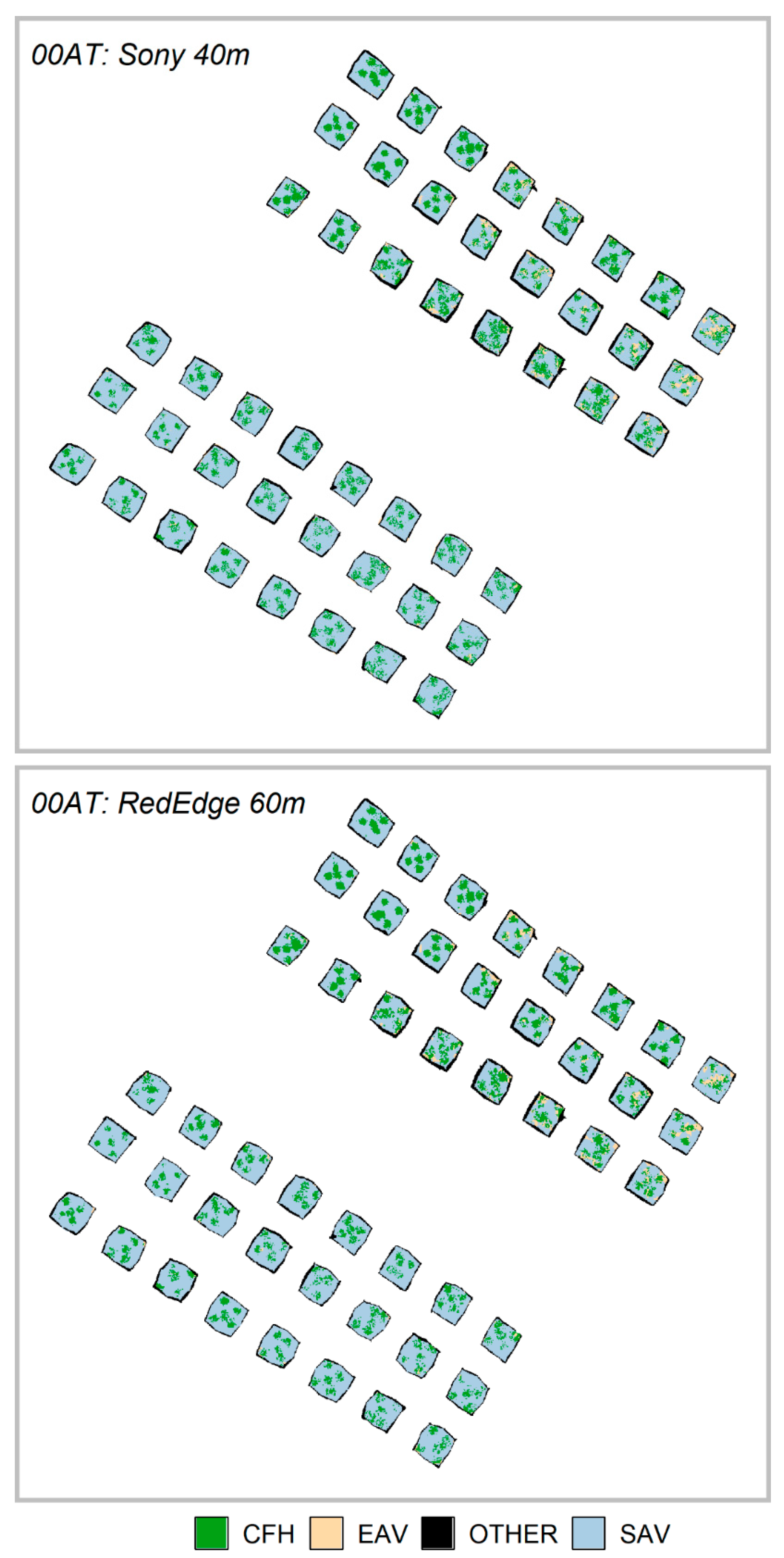
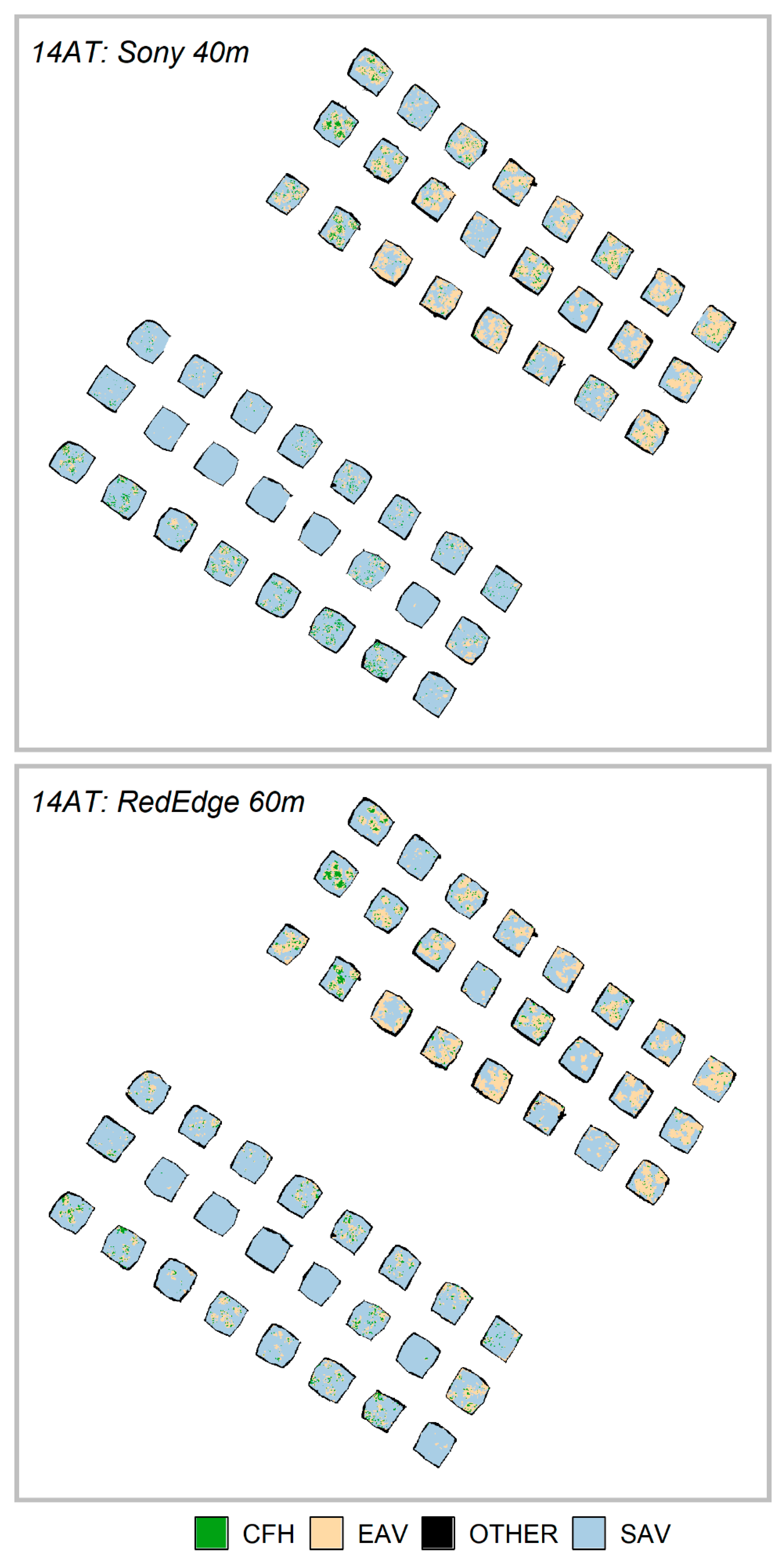
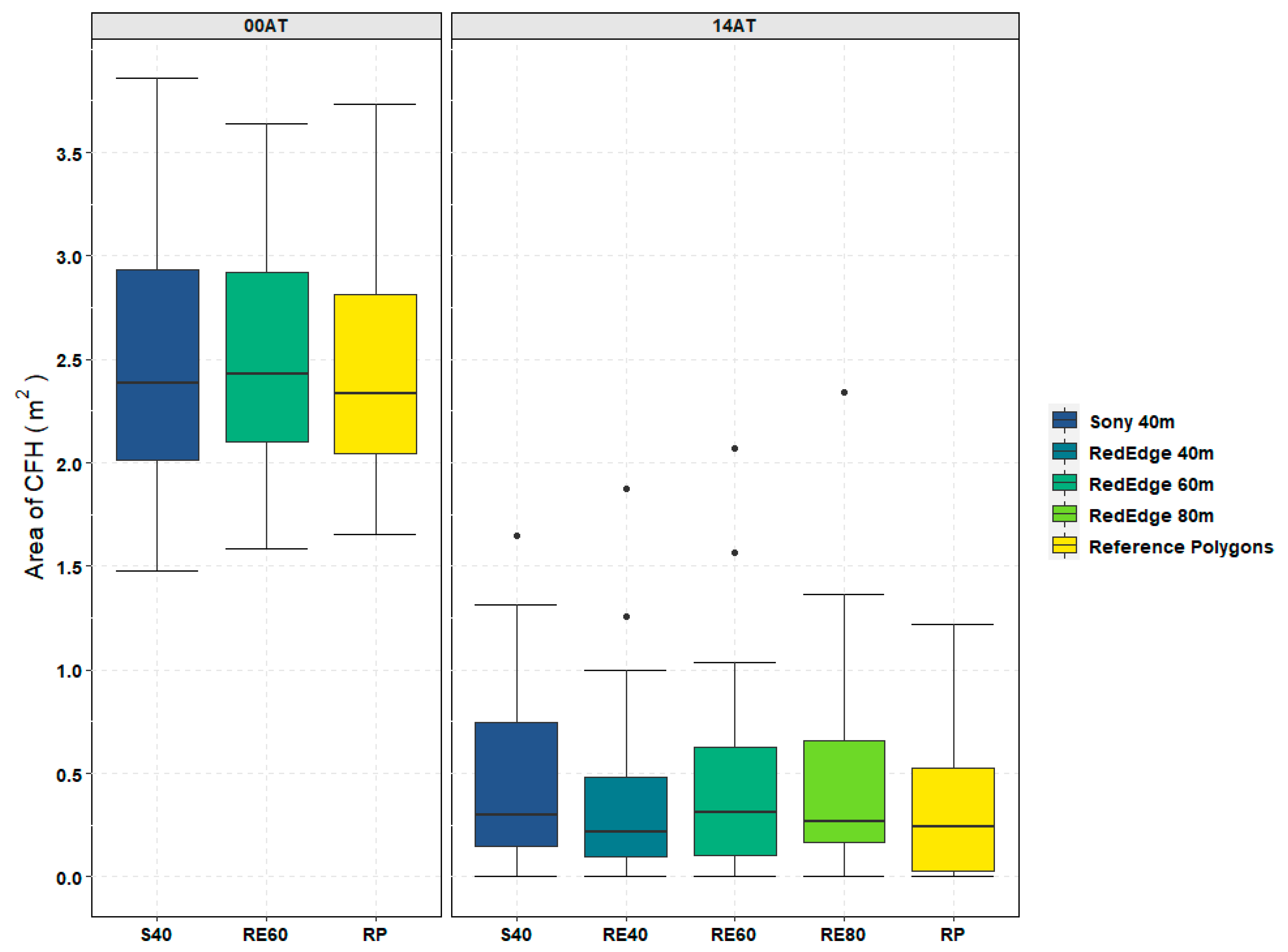
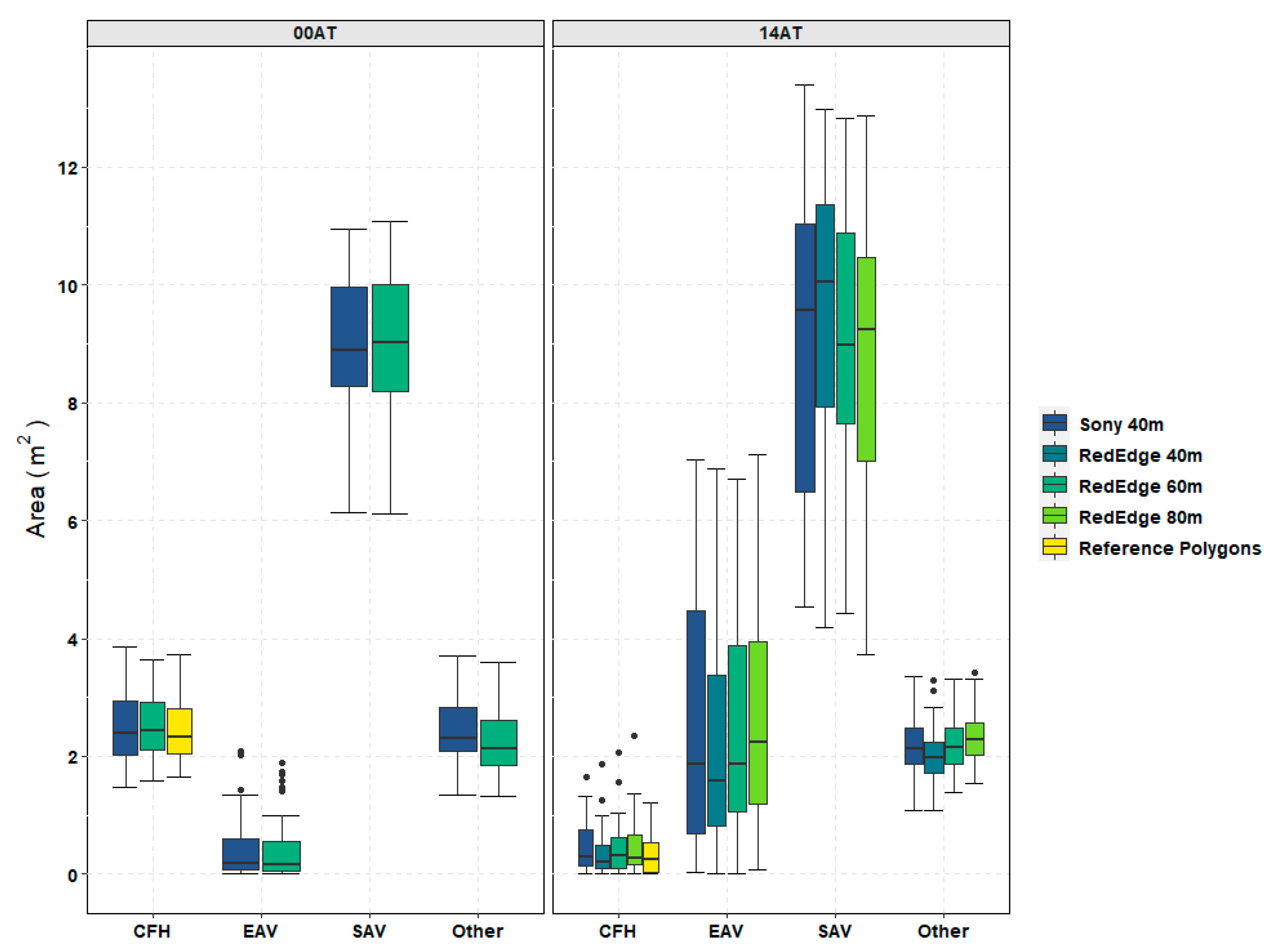
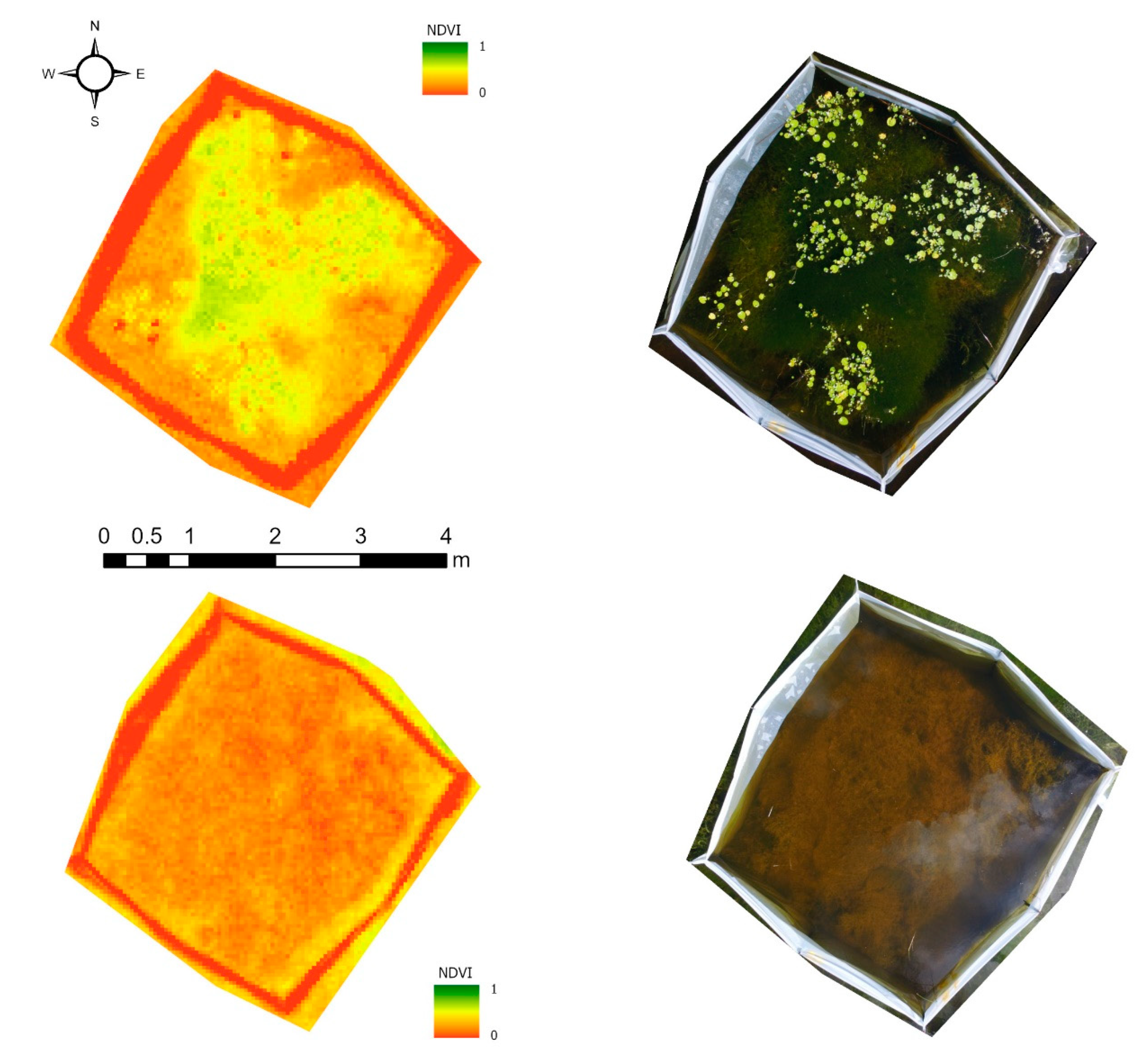
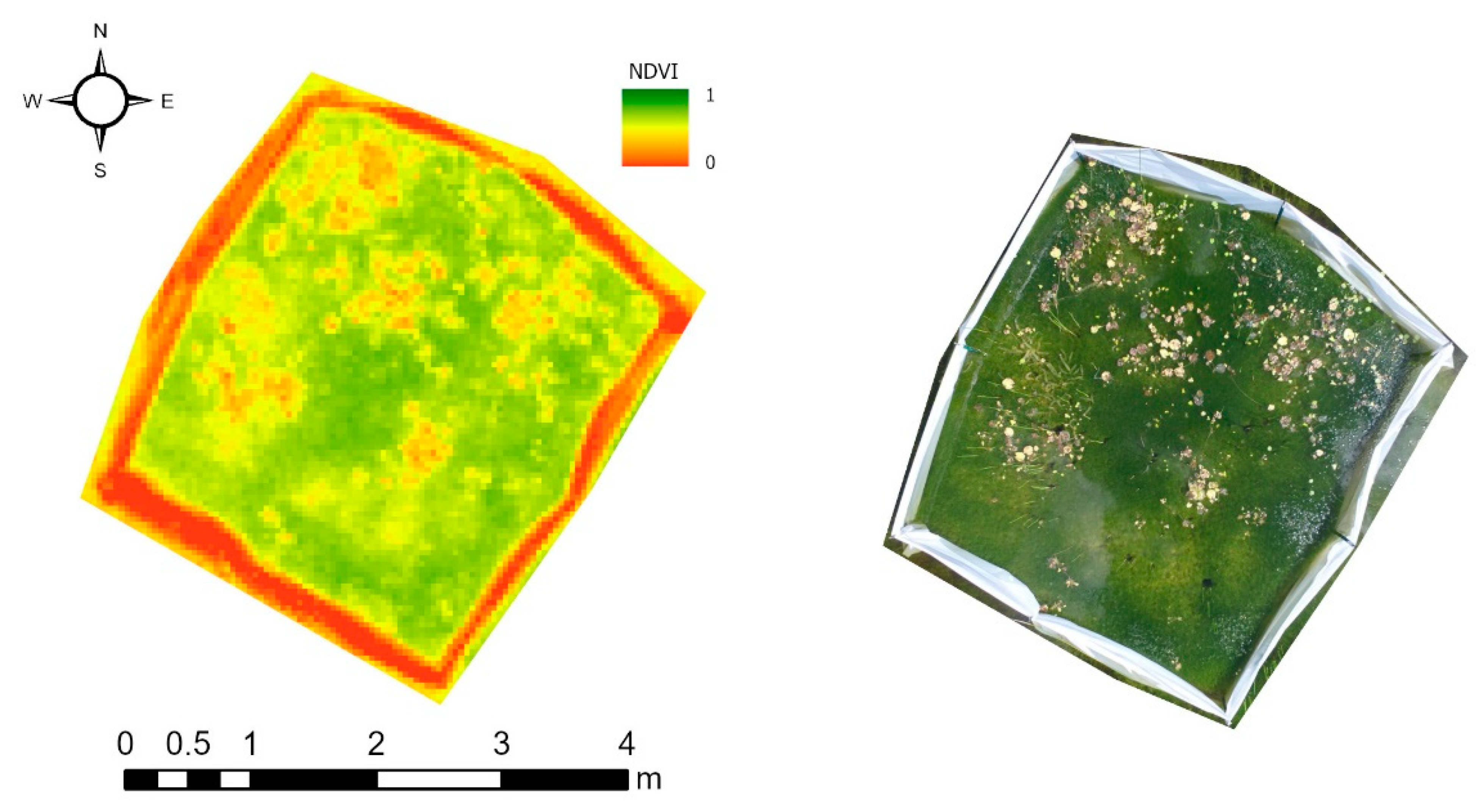
Table 3. This additional object information can be helpful in discriminating between vegetation and non-vegetation classes. During the 14AT trials, emergent aquatic vegetation (EAV) was more prevalent in the TPs than it was on 00AT as shown in Figure 9. Furthermore, the EAV and CFH classes were the most frequently confused classes in the accuracy assessment confusion matrices found in Table A1, Table A2, Table A3, Table A4, Table A5 and Table A6. The multispectral classified image derived from imagery at the lowest GSD (2.7 cm/pix at 40 m AGL) had the best performance in discriminating between these two vegetation classes as shown in Table A3. When comparing multispectral (2.7 cm/pix GSD) and RGB (1.7 cm/pix GSD) datasets collected at the same flight altitude (40 m), the results from the RE40 dataset showed a small but significant improvement in the accuracy of measuring areal coverage at a 95% confidence level. Based on the manufacturer’s recommendation, multispectral data was only collected at the flight altitude of 60 m (4.1 cm/pix GSD) for the pre-treatment assessment date (00AT). Thus, a comparison between datasets from the same flight altitude (40 m) was only conducted for 14AT where data was available.
While multispectral sensor performance showed statistically significant improvement over RGB-only datasets at certain spatial resolutions for accurately measuring areal coverage, water resource managers must also balance other operational considerations. The first consideration is cost. At present, prosumer drones (e.g., DJI Phantom series used herein) are approximately $1500 with standard visual cameras (e.g., Sony EXMOR) included in the price. Quality UAS multispectral cameras (e.g., MicaSense RedEdge) cost approximately $5000 without accounting for a stable UAS platform to carry the sensor. Suitable UAS platforms range in price from a few hundred to a few thousand dollars. Once startup costs are accounted for, operational considerations must be evaluated as well. Multispectral cameras such as the RedEdge typically have a limited field of view relative to standard optical cameras as shown in Table 1. To maintain the 70–80% image sidelap necessary for quality SfM-derived orthophoto mosaics, additional flight lines in the field are required [38]. This corresponds to both additional images and flight time as shown in Table 2. Consequently, data volume can differ considerably across sensors as well. The RedEdge sensor comprises five cameras, each operating on a different portion of the electromagnetic spectrum. For every image location, a single uncompressed 2.4 megabytes (MB) tif image is captured by each camera. Meanwhile, the Sony EXMOR camera captures the RGB bands in one compressed jpeg image that is approximately 5 MB in size. For this small 0.8 ha project, raw multispectral imagery collected at 40 m AGL on 14AT was approximately 1,980 MB of imagery files and the Sony imagery collected at the same 40 m AGL was 590 MB. While specifications certainly vary by sensor, UAS operators need to be cognizant of file storage and subsequent processing demands especially with multispectral imagery which is typically stored and processed in an uncompressed format. Thus, the implementation of multispectral imaging into a UAS operational workflow is not a trivial decision based purely on accuracy performance.
Similar to other UAS projects targeting specific vegetation species [43,
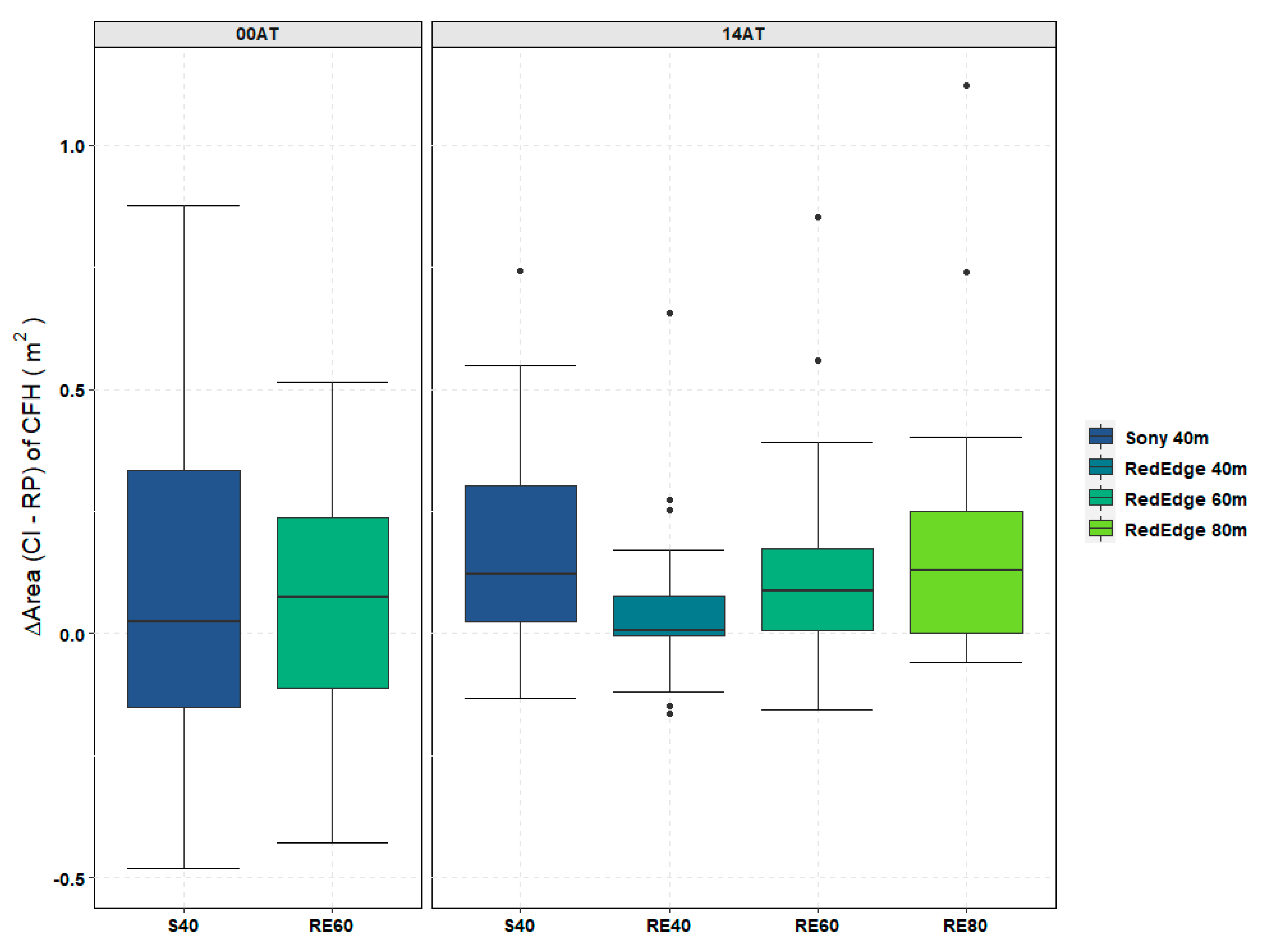
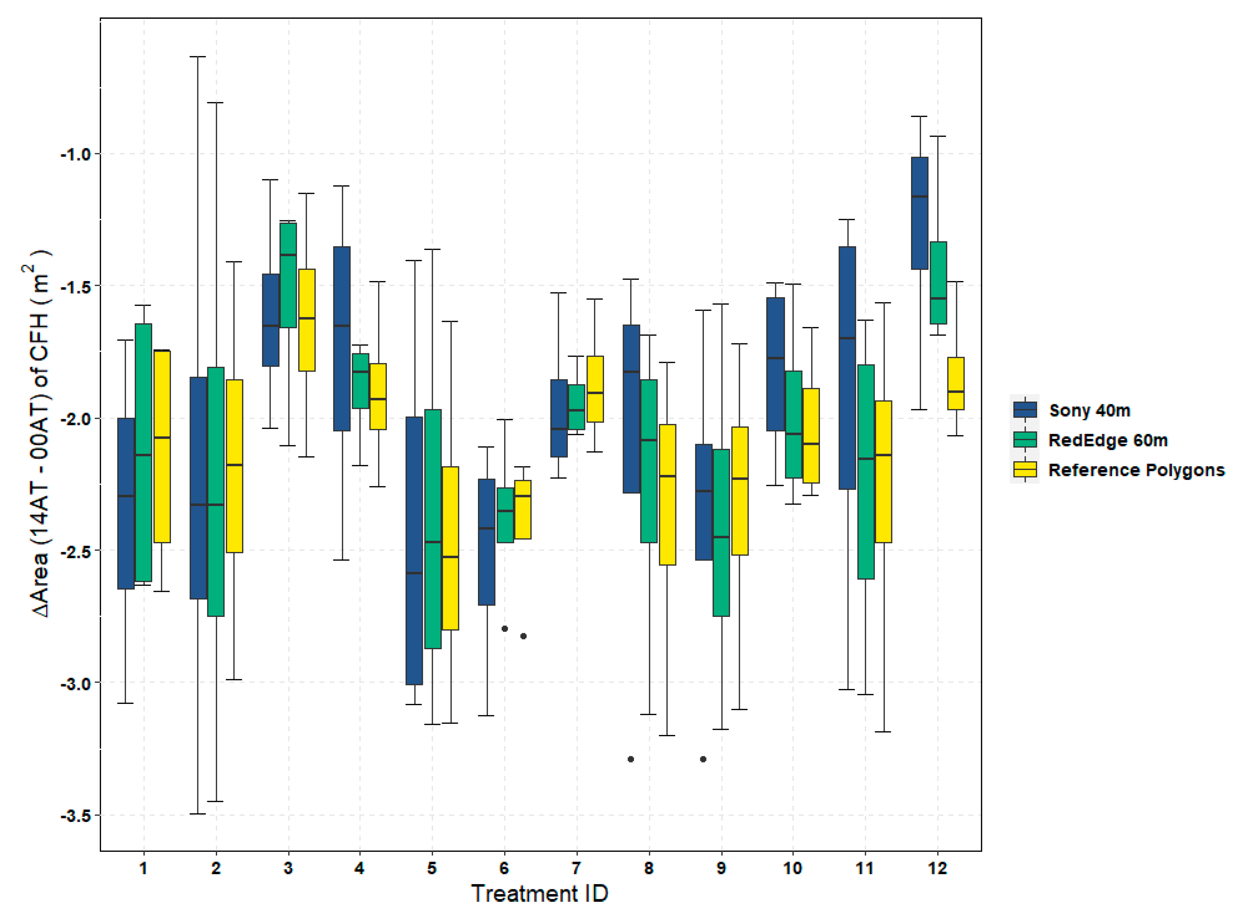
44], flight altitude and in turn GSD impacted the accuracy of CFH detection in this study. This is evidenced by the differences in CFH class accuracy from the classified image accuracy assessments (Table A4 and Table A6) as well as the small but significant difference in areal coverage accuracy (Figure 10) between the RedEdge trial flown at 40 m (RE40) and the RedEdge trial flown at 80 m (RE80). As a result, water resource managers must find an acceptable balance between potentially small but significant accuracy improvements noted above and the additional operational constraints imposed by achieving a higher spatial resolution. In this 0.8 ha study, the flight time for RE40 was nearly 10 min longer than the 7-min, RE80 flight as shown in Table 2. The lower flight altitude not only restricts the mission areal coverage per takeoff, but it also leads to increased volumes of data: 1,980 MB of imagery for RE40 versus 1,280 MB of imagery for RE80 on 14AT. Given these operational considerations and the ability to still obtain a high overall accuracy assessment (e.g., 89.6% with a 5.5 cm/pix GSD), many water resource managers may be willing to forego the marginal accuracy improvements of capturing data at a higher spatial resolution. One potential way to mitigate the time constraints of flying lower is to improve the spatial resolution of the multispectral sensor. For example, the newest, multispectral MicaSense sensor is the Altum, which offers a 50% improvement in spatial resolution relative to the MicaSense RedEdge [64]. Thus, operational efficiencies can be gained by flying 50% higher with the newer Altum sensor and maintaining the same GSD as the RedEdge. Alternatively, managers willing to forego the highest accuracies could fly the Altum at maximum allowable altitudes without a waiver (e.g., 121.9 m in the United States) to obtain a GSD of 5.3 cm/pix. With these operational parameters, UAS practitioners could reduce the amount of data acquired and subsequent SfM processing time while still creating high-accuracy datasets.
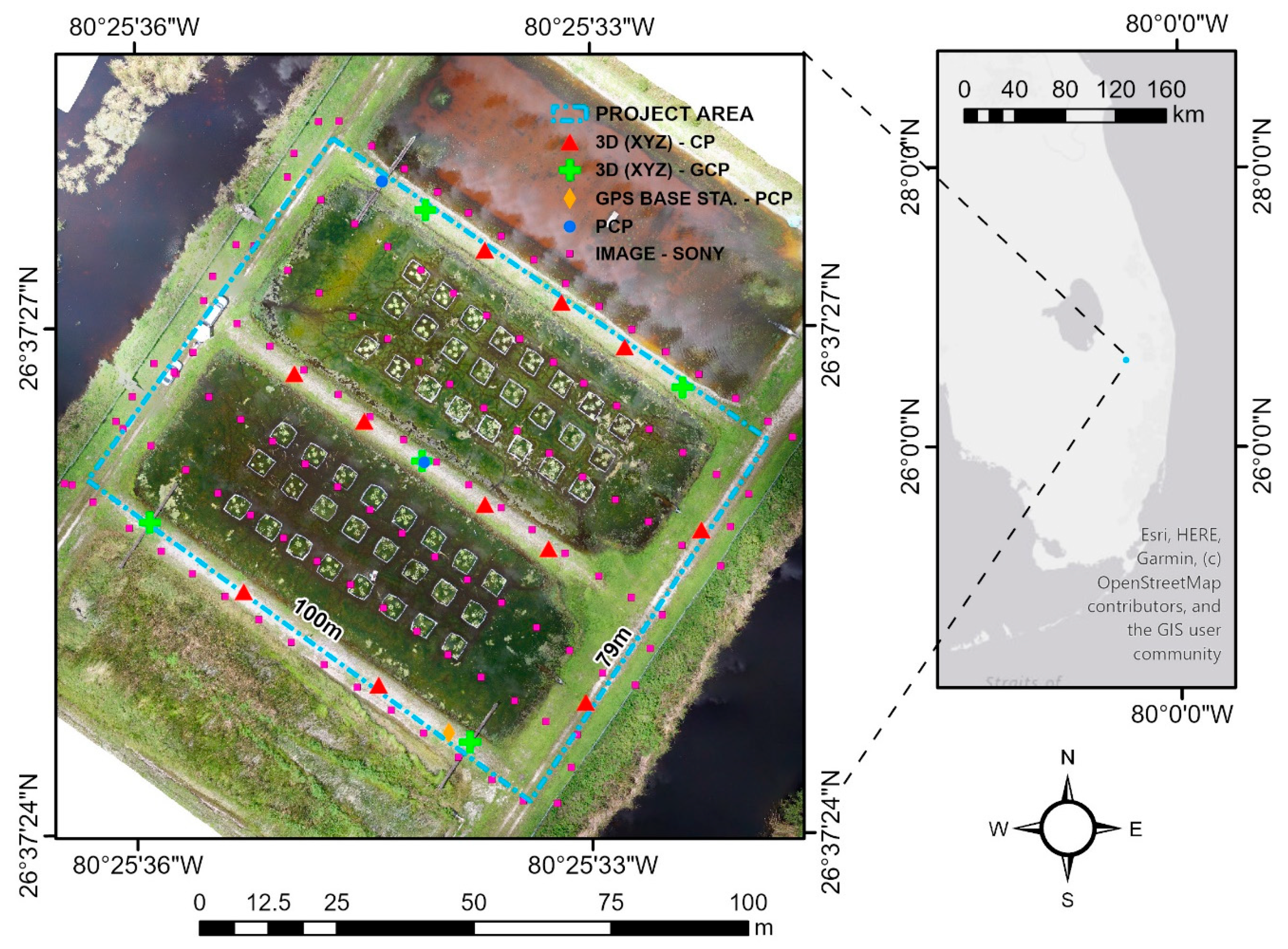
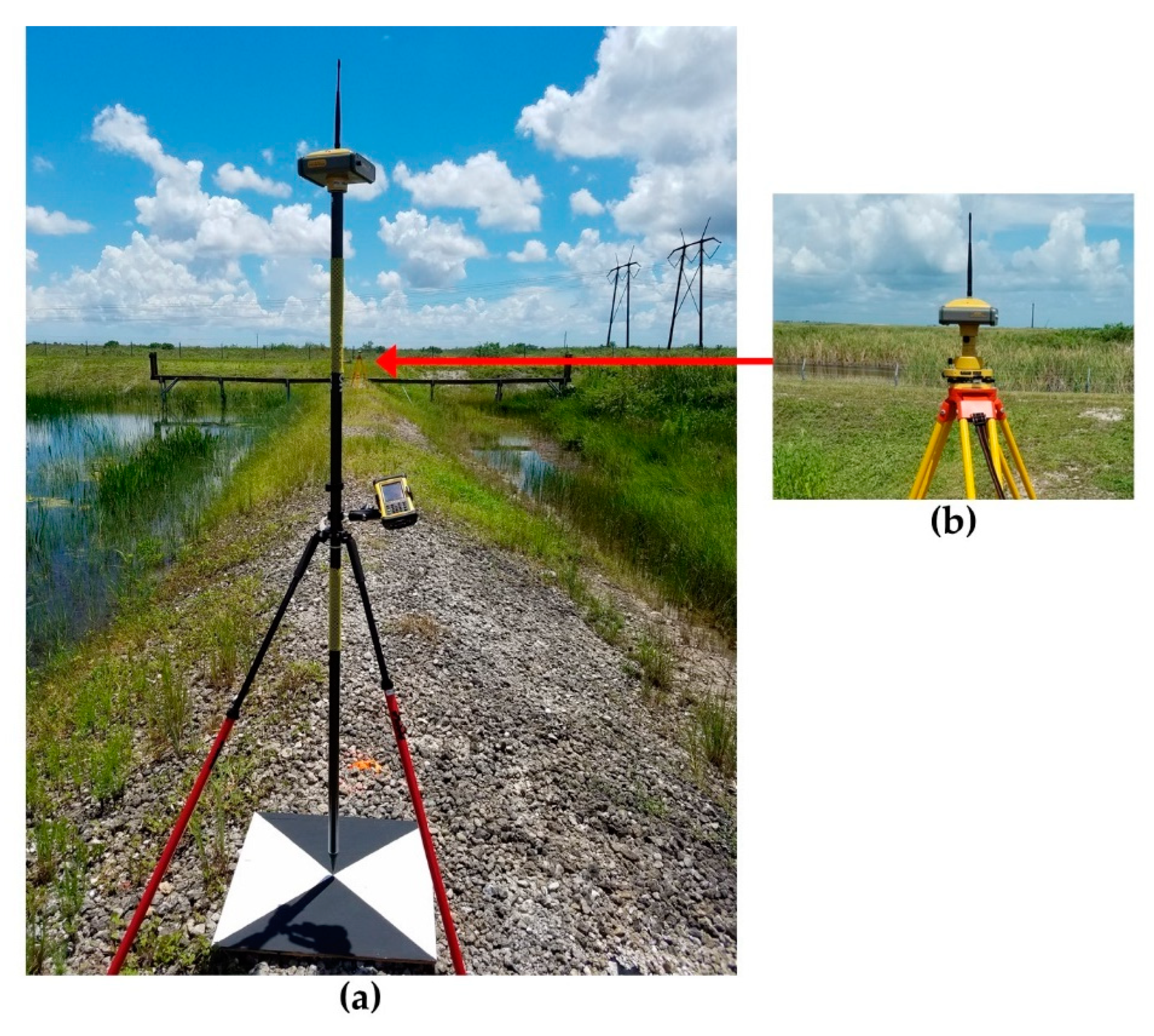
Even after optimizing operations through sensor selection and UAS flight planning parameters, multiple factors can still influence the accuracy of the results. For this project, the datasets were tightly georeferenced using stationary GCPs to ensure the best possible dataset alignment across the various trials. In a larger, natural wetland setting, access to well-distributed GCPs will be minimal. In these situations, georeferencing datasets using on-board, post-processed kinematic (PPK) GNSS can provide the best available positioning solution with misalignment errors similar to using GCPs [65,66,67]. The implementation of PPK GNSS requires either a PPK-enabled UAS platform or additional positioning sensors mounted to the existing UAS platform. Either scenario results in additional financial costs above and beyond the cost of the prosumer drone to mitigate dataset misalignment. During data acquisition, a poor sun angle can cause sun glint on the water surface. Sun glint can cause misalignments in the SfM processing, potentially adversely impacting the accuracy of resultant classified imagery [51,68].
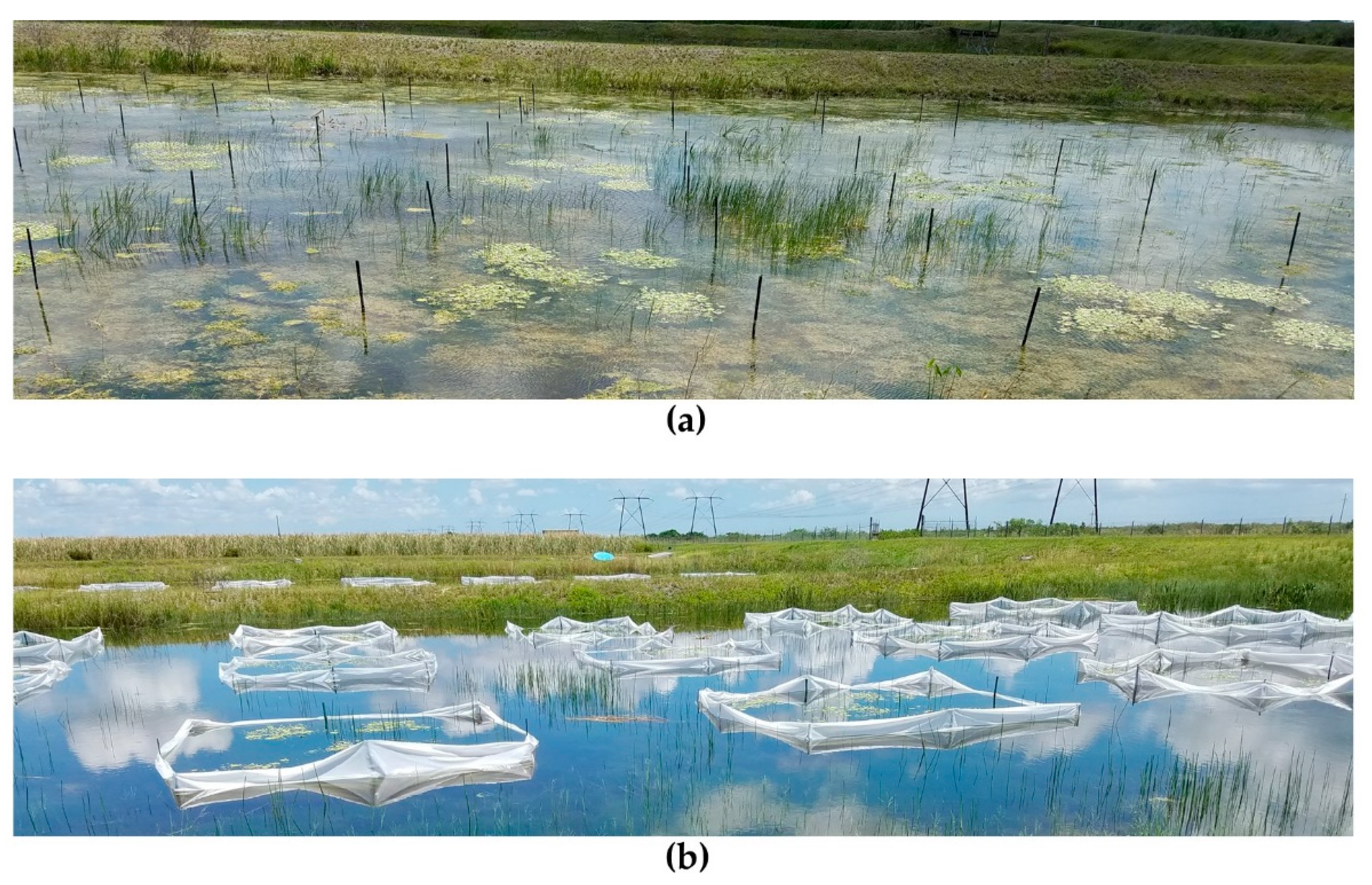
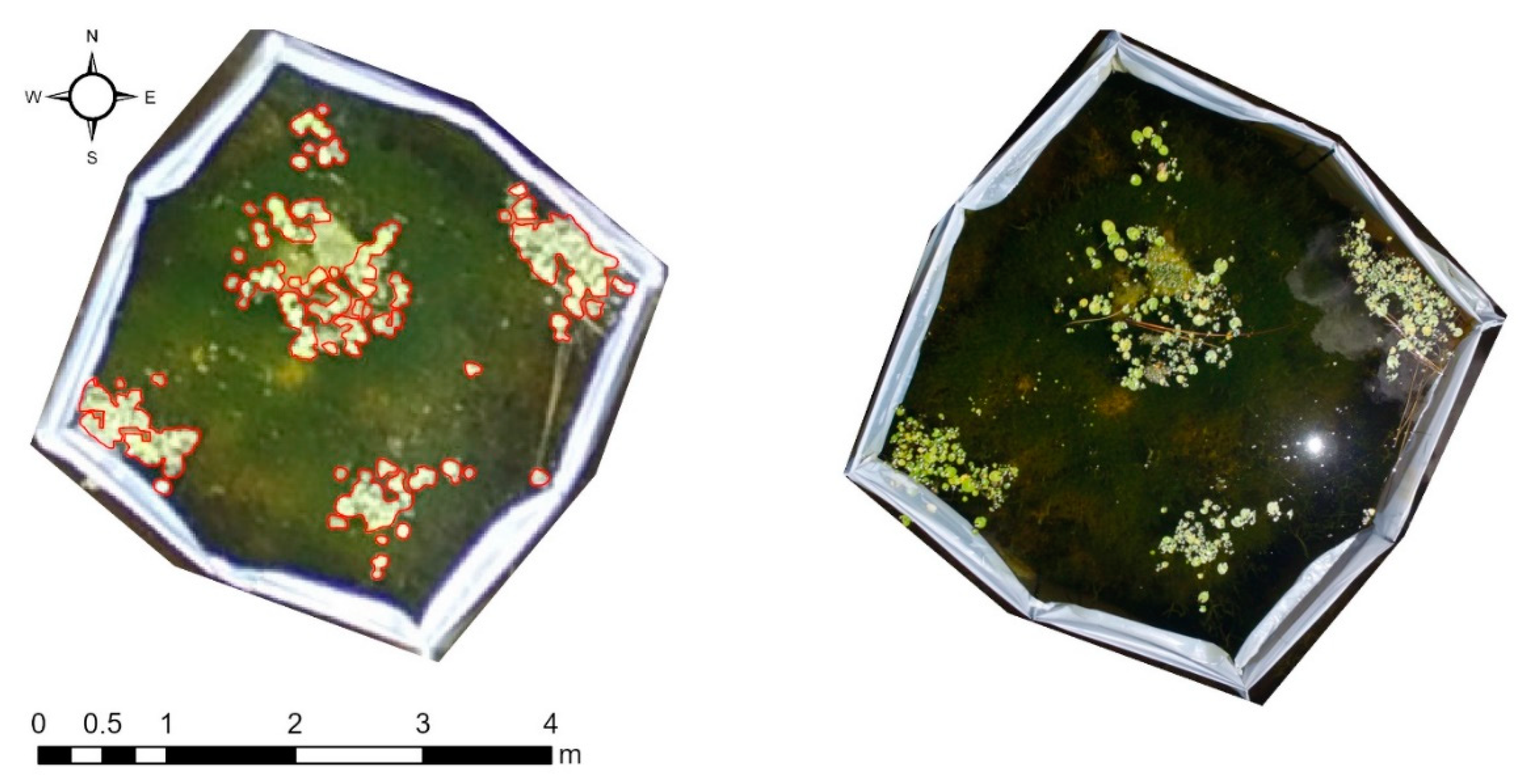
Another environmental factor that impacts floating wetland vegetation more so than terrestrial vegetation is vegetation movement. While FLAV is tethered to the bottom, the vegetation is still susceptible to drift on the water’s surface. This can cause individual vegetation leaves to cluster or disperse depending on water and wind currents. When plants disperse, the spatial resolution of the imagery must be high enough to capture individual leaves on the water surface, or underestimation of invasive vegetation will result. Meanwhile, plants that cluster together can cause overlapping leaves and in turn, result in underestimation of the subject vegetation class area coverage as well. While some field conditions can be mitigated (e.g., sun angle planning, PPK implementation), there is inherent noise in the classified image datasets that water resource managers need to be aware of when integrating UAS mapping and analysis in the decision-making process.

4.2. Future Considerations

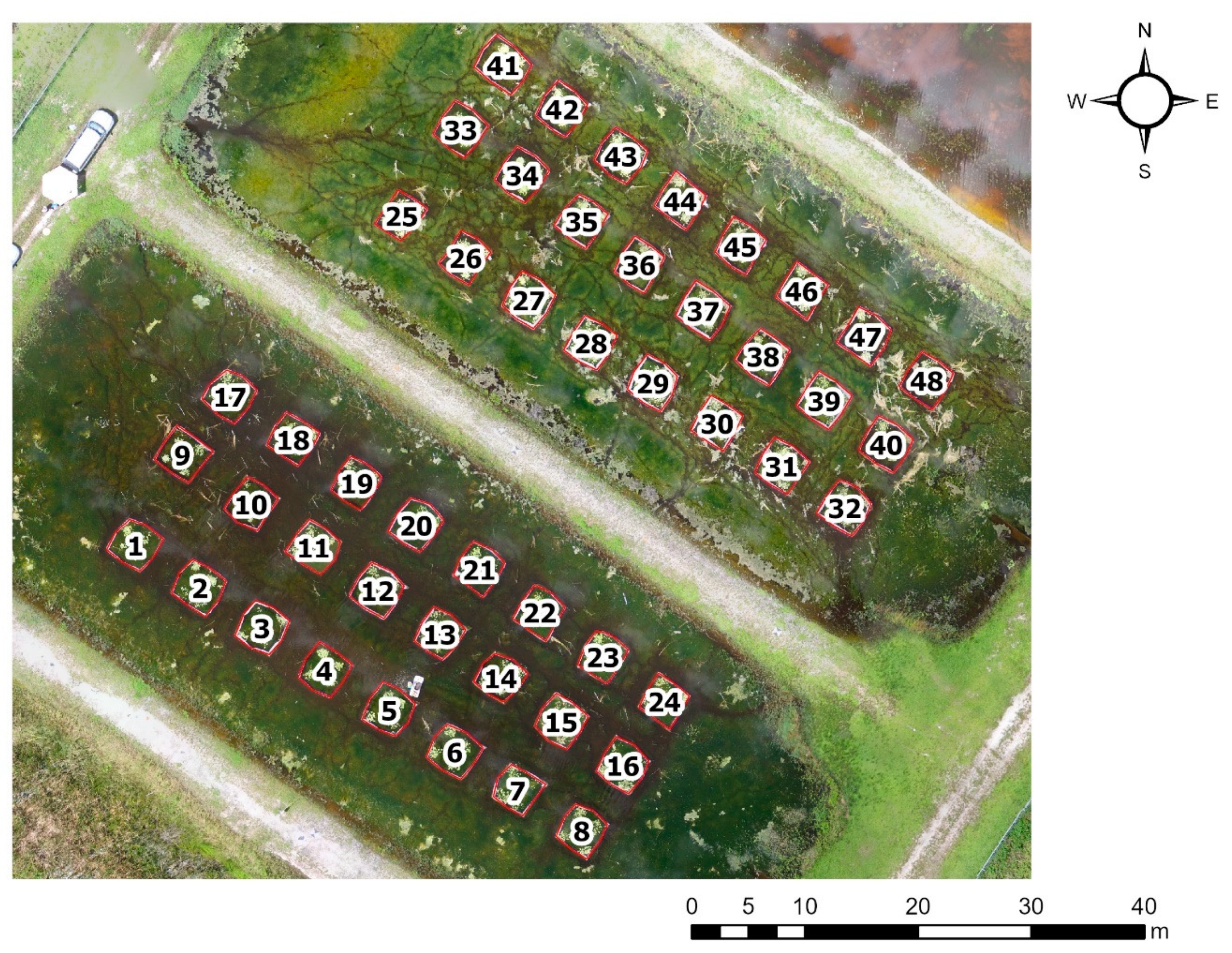
To effectively study herbicide efficacy on highly invasive vegetation in a randomized block design field trial, meticulous planning went into planting equal amounts of CFH in each TP and subsequently containing the CFH from entering the larger wetland complex surrounding the treatment ponds. Hence, water flow was restricted to the treatment ponds and plastic sheeting was used to form a physical barrier surrounding each TP and the subject vegetation. Due to these constraints, there was less mixing of invasive and native wetland vegetation than would be encountered when finding CFH in natural areas. A field study that investigates the management of CFH in a natural setting similar to Lishawa et al. [69], which investigated the management of Typha spp., would be the next progression in determining the value that multispectral remote sensing adds when water resource managers are faced with greater vegetative biodiversity than encountered in this project.
Thus far, CFH was accurately detected at all spatial resolutions tested in this project. A natural progression would be to further optimize data acquisition efficiency by collecting lower spatial resolution, multispectral imagery with the RedEdge sensor (e.g., 6.8 cm/pix at 100 m AGL, 8.3 cm/pix at 121.9 m AGL) and with the Sony sensor (e.g., 2.6 cm/pix at 60 m AGL, 3.4 cm/pix at 80 m AGL). If CFH communities can still be mapped accurately at these lower resolutions, water resource managers would have additional opportunities to reduce processing time and the amount of data acquired. Other data acquisition (e.g., image sidelap/overlap) and image processing (e.g., segmentation and classification parameters) variables were standardized for this project, but further investigation may yield additional accuracy improvements. On the data collection side, the sidelap and overlap parameters were each set to 80% for both sensors to ensure that no issues were encountered during SfM alignment and subsequent orthophoto mosaic generation. Reducing the sidelap parameter would reduce the number of flight lines leading to reductions in data acquisition time and the volume of data acquired. To test, a water resource manager could run a sample experiment by collecting UAS imagery at an extremely high sidelap of 90% or 95%. During SfM processing, datasets could be generated using every other or every third flightline to find the point at which the final classified imagery accuracy degrades for the given wetland environment and target vegetation species. This could help optimize data collection for temporal monitoring of larger areas with similar landcover characteristics.
The image processing parameters were standardized during the image segmentation and image classification process. Given prior studies on the superior performance of RF classifiers for OBIA land cover classification [60], testing of additional classifier algorithms was not undertaken. Furthermore, while additional testing of RF parameters and object features may yield improvements in the accuracy assessment of the classified images, these improvements if significant would be minimal given the high overall accuracy assessments found in Table 4. For future consideration, the feature objects of importance for the RF classifier were exported from eCognition. The mean values for the green and blue bands and the indices (i.e., NDVI, VDVI, VB) were most important for object classification. Meanwhile, the standard deviation value of the spectral bands, the mean and standard deviation of the DSM, and the GLCM Dissimilarity object feature were characterized as the least important. The relative importance of these object features may be applicable going forward for subsequent monitoring studies of similar FLAV species especially when considering the use of band indices for discriminating between vegetation and non-vegetation classes [29,43,44,48].
As the fields of deep learning and artificial intelligence continue to evolve, the adoption of these approaches to temporal vegetation monitoring is certainly encouraged [49]. For larger monitoring projects of invasive vegetation management techniques, a deep learning framework incorporating high-resolution UAS imagery as the training data for satellite imagery would be a valuable tool for water resource managers. The success of previous studies expanding the scale of remote sensing projects through the fusion of datasets from multiple sensor types provides additional support for this effort [28,30].

5. Conclusions

This study provides a more thorough understanding of UAS sensor selection and UAS data acquisition for monitoring the effectiveness of invasive aquatic vegetation management strategies. CFH (Nymphoides cristata), a floating-leaved aquatic plant, was the focal invasive vegetation species investigated herein due to its rapid growth potential in the southeastern US. Through investigation of OBIA classified images, the only significant difference in area coverage accuracy at a 95% confidence level amongst the six trials was a small improvement in accuracy between the 40 m multispectral (2.7 cm/pix GSD) and the 40 m RGB-only (1.7 cm/pix GSD) datasets. When comparing temporal area change between treatment day and two weeks post-treatment, there was no statistically significant difference between the change in area derived from the reference polygons and change in area derived from the other two trial pairs (multispectral with 4.1 cm/pix GSD and RGB-only with 1.7 cm/pix GSD). Based on these results, water resource managers can have confidence in the adoption of an object-based UAS remote sensing workflow for vegetation species detection and vegetation community areal change assessment when monitoring invasive aquatic vegetation management strategies. Finally, additional UAS operational considerations (e.g., cost, time, data storage) related to flight planning and sensor selection were provided to guide decision-making on the adoption of multispectral UAS remote sensing for a given monitoring application.

Author Contributions

A.R.B. conceived the study. L.A.G. and K.T. designed and set up the field site for the herbicide treatment trials. A.R.B. collected and processed the UAS and GNSS data. A.R.B. and A.A.-E. analyzed the data. A.R.B. wrote the original manuscript. A.R.B., A.A.-E., L.A.G., H.H.H. and K.T. contributed with writing, reviewing, and editing subsequent versions of the manuscript. All authors have read and agreed to the published version of the manuscript.

Funding

This research received no external funding.

Institutional Review Board Statement

Not applicable.

Informed Consent Statement

Not applicable.

Data Availability Statement

The data presented in this study are available on request from the corresponding author.

Acknowledgments

Thank you to the South Florida Water Management District for access to the field site in Stormwater Treatment Area 1-West. Thank you to Ian Markovich, Mohsen Tootoonchi, and Joseph Sigmon for field site construction and data collection support. Thank you to the anonymous reviewers who provided detailed feedback that guided the improvement of this manuscript during the review process.

Conflicts of Interest

The authors declare no conflict of interest.

Appendix A

Table A1. Accuracy assessment confusion matrix for the OBIA RF classification results from 0AT with the Sony sensor and a 1.7 cm/pix GSD.
Ground Truth/Reference
ClassCFHSAVEAVOtherTotalUser’s Acc.Commiss. Error
CFH79120820.9630.037
SAV07911810.9750.025
EAV70253350.7140.286
Other01041420.9760.024
Total86812845
Producer’s Acc.0.9190.9750.8930.911 Overall Acc.0.933
Omission Error0.0810.0250.1070.089 Kappa0.907
Table A2. Accuracy assessment confusion matrix for the OBIA RF classification results from 0AT with the MicaSense RedEdge and a 4.1 cm/pix GSD.
Ground Truth/Reference
ClassCFHSAVEAVOtherTotalUser’s Acc.Commiss. Error
CFH77120800.9630.038
SAV17801800.9750.025
EAV65272400.6750.325
Other00040401.0000.000
Total84842943
Producer’s Acc.0.9170.9290.9310.930 Overall Acc.0.925
Omission Error0.0830.0710.0690.070 Kappa0.895
Table A3. Accuracy assessment confusion matrix for the OBIA RF classification results from 14AT with the Sony sensor and a 1.7 cm/pix GSD.
Ground Truth/Reference
ClassCFHSAVEAVOtherTotalUser’s Acc.Commiss. Error
CFH691100800.8630.138
SAV07820800.9750.025
EAV25303400.7500.250
Other01138400.9500.050
Total71854341
Producer’s Acc.0.9720.9180.6980.927 Overall Acc.0.896
Omission Error0.0280.0820.3020.073 Kappa0.856
Table A4. Accuracy assessment confusion matrix for the OBIA RF classification results from 14AT with the MicaSense RedEdge and a 2.7 cm/pix GSD.
Ground Truth/Reference
ClassCFHSAVEAVOtherTotalUser’s Acc.Commiss. Error
CFH73070800.9130.088
SAV07910800.9880.013
EAV11380400.9500.050
Other00139400.9750.025
Total74804739
Producer’s Acc.0.9860.9880.8091.000 Overall Acc.0.954
Omission Error0.0140.0130.1910.000 Kappa0.937
Table A5. Accuracy assessment confusion matrix for the OBIA RF classification results from 14AT with the MicaSense RedEdge and a 4.1 cm/pix GSD.
Ground Truth/Reference
ClassCFHSAVEAVOtherTotalUser’s Acc.Commiss. Error
CFH70262800.8750.125
SAV07910800.9880.013
EAV05341400.8500.150
Other10138400.9500.050
Total71864241
Producer’s Acc.0.9860.9190.8100.927 Overall Acc.0.921
Omission Error0.0140.0810.1900.073 Kappa0.891
Table A6. Accuracy assessment confusion matrix for the OBIA RF classification results from 14AT with the MicaSense RedEdge and a 5.5 cm/pix GSD.
Ground Truth/Reference
ClassCFHSAVEAVOtherTotalUser’s Acc.Commiss. Error
CFH690110800.8630.138
SAV07721800.9630.038
EAV74290400.7250.275
Other00040401.0000.000
Total76814241
Producer’s Acc.0.9080.9510.6900.976 Overall Acc.0.896
Omission Error0.0920.0490.3100.024 Kappa0.856

References

  1. Silva, T.S.F.; Costa, M.P.F.; Melack, J.M.; Novo, E.M.L.M. Remote sensing of aquatic vegetation: Theory and applications. Environ. Monit. Assess. 2008, 140, 131–145. [Google Scholar] [CrossRef]
  2. Boerema, A.; Schoelynck, J.; Bal, K.; Vrebos, D.; Jacobs, S.; Staes, J.; Meire, P. Economic valuation of ecosystem services, a case study for aquatic vegetation removal in the Nete catchment (Belgium). Ecosyst. Serv. 2014, 7, 46–56. [Google Scholar] [CrossRef]
  3. Florida Exotic Pest Plant Council (FLEPPC). Florida Exotic Pest Plant Council’s 2019 List of Invasive Plant Species; Florida Exotic Pest Plant Council: Gainesville, FL, USA, 2019; pp. 1–4. Available online: https://bugwoodcloud.org/CDN/fleppc/plantlists/2019/2019_Plant_List_ABSOLUTE_FINAL.pdf (accessed on 2 December 2020).
  4. Hershner, C.; Havens, K.J. Managing Invasive Aquatic Plants in a Changing System: Strategic Consideration of Ecosystem Services. Conserv. Biol. 2008, 22, 544–550. [Google Scholar] [CrossRef] [PubMed]
  5. Lakewatch. A Beginner’s Guide to Water Management—Aquatic Plants in Florida Lakes; EDIS; Fisheries & Aquatic Sciences, Florida Cooperative Extension Service, Institute of Food and Agricultural Sciences, University of Florida: Gainesville, FL, USA, 2017; pp. 1–43. Available online: http://edis.ifas.ufl.edu/pdffiles/FA/FA16300.pdf (accessed on 2 December 2020).
  6. Sun, J.; Wang, L.; Ma, L.; Huang, T.; Zheng, W.; Min, F.; Zhang, Y.; Wu, Z.; He, F. Determinants of submerged macrophytes palatability to grass carp Ctenopharyngodon idellus. Ecol. Indic. 2018, 85, 657–663. [Google Scholar] [CrossRef]
  7. Jones, R.W.; Hill, J.M.; Coetzee, J.A.; Hill, M.P. The contributions of biological control to reduced plant size and biomass of water hyacinth populations. Hydrobiologia 2018, 807, 377–388. [Google Scholar] [CrossRef]
  8. Gettys, L.A.; Torre, C.J.D., III. Rotala: A New Aquatic Invader in Southern Florida; UF/IFAS Extension—University of Florida: Gainesville, FL, USA, 2017; pp. 1–4. Available online: https://edis.ifas.ufl.edu/pdffiles/AG/AG38100.pdf (accessed on 2 December 2020).
  9. Lovell, S.J.; Stone, S.F.; Fernandez, L. The Economic Impacts of Aquatic Invasive Species: A Review of the Literature. Agric. Resour. Econ. Rev. 2006, 35, 195–208. [Google Scholar] [CrossRef]
  10. Getsinger, K.; Dibble, E.; Rodgers, J.; Spencer, D. Benefits of Controlling Nuisance Aquatic Plants and Algae in the United States; CAST: Ames, IA, USA, 2014; pp. 1–12. Available online: https://www.cast-science.org/wp-content/uploads/2018/12/Aquatic_Plants_final_QTA20141_0121E9C2A73B5.pdf (accessed on 14 December 2020).
  11. Florida Exotic Pest Plant Council (FLEPPC). Florida Exotic Pest Plant Council’s 2009 List of Invasive Plant Species; Florida Exotic Pest Plant Council: Gainesville, FL, USA, 2009; pp. 1–4. Available online: https://www.fleppc.org/list/2009/List-WW-F09-final.pdf (accessed on 2 December 2020).
  12. Gettys, L.A.; Torre, C.J.D., III; Thayer, K.; Markovich, I.J. Asexual reproduction and ramet sprouting of crested floatingheart (Nymphoides cristata). J. Aquat. Plant Manag. 2017, 55, 83–88. [Google Scholar]
  13. Florida Department of Agriculture and Consumer Services (FDACS). Chapter 5B–57 Introduction or Release of Plant Pests, Noxious Weeds, Arthropods, and Biological Control Agents; Florida Department of Agriculture and Consumer Services: Tallahassee, FL, USA, 2020; pp. 1–15. Available online: https://www.flrules.org/gateway/ChapterHome.asp?Chapter=5B-57 (accessed on 7 December 2020).
  14. Floatinghearts. Biology and Control of Aquatic Plants: A Best Management Practices Handbook; Aquatic Ecosystem Restoration Foundation: Marietta, GA, USA, 2020; pp. 59–64. Available online: http://aquatics.org/bmpchapters/BMP4ed.pdf (accessed on 7 December 2020).
  15. Gettys, L.A. Waterhyacinth: Florida’s Worst Floating Weed; EDIS; Agronomy Department, Florida Cooperative Extension Service, Institute of Food and Agricultural Sciences, University of Florida: Gainesville, FL, USA, 2017; pp. 1–5. Available online: https://edis.ifas.ufl.edu/pdffiles/AG/AG38500.pdf (accessed on 18 November 2020).
  16. Willey, L.N.; Langeland, K.A. Aquatic Weeds: Crested Floating Heart (Nymphoides cristata); EDIS; Agronomy Department, Florida Cooperative Extension Service, Institute of Food and Agricultural Sciences, University of Florida: Gainesville, FL, USA, 2014; pp. 1–4. Available online: https://edis.ifas.ufl.edu/pdffiles/AG/AG35400.pdf (accessed on 2 December 2020).
  17. Harms, N.; Nachtrieb, J. Suitability of Introduced Nymphoides spp. (Nymphoides cristata, N. peltata) as Targets for Biological Control in the United States; Engineer Research and Development Center (U.S.): Vicksburg, MS, USA, 2019; Available online: https://erdc-library.erdc.dren.mil/jspui/handle/11681/32347 (accessed on 2 December 2020).
  18. Glomski, L.M.; Willey, L.N.; Netherland, M.D. The efficacy of protox-inhibiting herbicides alone and in combination with glyphosate to control crested floating heart. J. Aquat. Plant Manag. 2014, 52, 90–92. [Google Scholar]
  19. Glomski, L.; Netherland, M.D. Impact of herbicide retention time on the efficacy of foliar treatments for control of crested floating heart. J. Aquat. Plant Manag. 2016, 54, 50–52. [Google Scholar]
  20. Willey, L.N.; Netherland, M.D.; Haller, W.T.; Langeland, K.A. Evaluation of aquatic herbicide activity against crested floating heart. J. Aquat. Plant Manag. 2014, 52, 47–56. [Google Scholar]
  21. Valley, R.D.; Drake, M.T.; Anderson, C.S. Evaluation of alternative interpolation techniques for the mapping of remotely-sensed submersed vegetation abundance. Aquat. Bot. 2005, 81, 13–25. [Google Scholar] [CrossRef]
  22. Winfield, I.J.; van Rijn, J.; Valley, R.D. Hydroacoustic quantification and assessment of spawning grounds of a lake salmonid in a eutrophicated water body. Ecol. Inform. 2015, 30, 235–240. [Google Scholar] [CrossRef] [Green Version]
  23. Ozesmi, S.L.; Bauer, M.E. Satellite remote sensing of wetlands. Wetl. Ecol. Manag. 2002, 10, 381–402. [Google Scholar] [CrossRef]
  24. Madsen, J.D.; Wersal, R.M. A review of aquatic plant monitoring and assessment methods. J. Aquat. Plant Manag. 2017, 55, 1–12. [Google Scholar]
  25. Wu, L. (SFWMD Goals for Remote Sensing of SAV & EAV). Personal communication. 2019. [Google Scholar]
  26. Chabot, D.; Dillon, C.; Ahmed, O.; Shemrock, A. Object-based analysis of UAS imagery to map emergent and submerged invasive aquatic vegetation: A case study. J. Unmanned Veh. Syst. 2016, 5, 27–33. [Google Scholar] [CrossRef] [Green Version]
  27. Chabot, D.; Dillon, C.; Shemrock, A.; Weissflog, N.; Sager, E.P.S. An Object-Based Image Analysis Workflow for Monitoring Shallow-Water Aquatic Vegetation in Multispectral Drone Imagery. ISPRS Int. J. Geo-Inf. 2018, 7, 294. [Google Scholar] [CrossRef] [Green Version]
  28. Díaz-Delgado, R.; Cazacu, C.; Adamescu, M. Rapid Assessment of Ecological Integrity for LTER Wetland Sites by Using UAV Multispectral Mapping. Drones 2019, 3, 3. [Google Scholar] [CrossRef] [Green Version]
  29. Pande-Chhetri, R.; Abd-Elrahman, A.; Liu, T.; Morton, J.; Wilhelm, V.L. Object-based classification of wetland vegetation using very high-resolution unmanned air system imagery. Eur. J. Remote Sens. 2017, 50, 564–576. [Google Scholar] [CrossRef] [Green Version]
  30. Sartain, B.T.; Fleming, J.P.; Mudge, C.R. Utilizing remote sensing technology for monitoring chemically managed giant salvinia (Salvinia molesta) populations. J. Aquat. Plant Manag. 2019, 57, 14–22. [Google Scholar]
  31. Zweig, C.L.; Burgess, M.A.; Percival, H.F.; Kitchens, W.M. Use of Unmanned Aircraft Systems to Delineate Fine-Scale Wetland Vegetation Communities. Wetlands 2015, 35, 303–309. [Google Scholar] [CrossRef]
  32. Aasen, H.; Honkavaara, E.; Lucieer, A.; Zarco-Tejada, P.J. Quantitative Remote Sensing at Ultra-High Resolution with UAV Spectroscopy: A Review of Sensor Technology, Measurement Procedures, and Data Correction Workflows. Remote Sens. 2018, 10, 1091. [Google Scholar] [CrossRef] [Green Version]
  33. Manfreda, S.; McCabe, M.F.; Miller, P.E.; Lucas, R.; Madrigal, V.P.; Mallinis, G.; Dor, E.B.; Helman, D.; Estes, L.; Ciraolo, G.; et al. On the Use of Unmanned Aerial Systems for Environmental Monitoring. Remote Sens. 2018, 10, 641. [Google Scholar] [CrossRef] [Green Version]
  34. Thomas, O.H.; Smith, C.E.; Wilkinson, B.E. Economics of Mapping Using Small Manned and Unmanned Aerial Vehicles. Photogramm. Eng. Remote Sens. 2017, 83, 581–591. [Google Scholar] [CrossRef]
  35. Benjamin, A.; O’Brien, D.; Barnes, G.; Wilkinson, B.; Volkmann, W. Assessment of Structure from Motion (SfM) processing parameters on processing time, spatial accuracy, and geometric quality of unmanned aerial system derived mapping products. J. Unmanned Aer. Syst. 2017, 3, 73–99. [Google Scholar]
  36. Colomina, I.; Molina, P. Unmanned aerial systems for photogrammetry and remote sensing: A review. ISPRS J. Photogramm. Remote Sens. 2014, 92, 79–97. [Google Scholar] [CrossRef] [Green Version]
  37. Pajares, G. Overview and Current Status of Remote Sensing Applications Based on Unmanned Aerial Vehicles (UAVs). Photogramm. Eng. Remote Sens. 2015, 81, 281–330. [Google Scholar] [CrossRef] [Green Version]
  38. Singh, K.K.; Frazier, A.E. A meta-analysis and review of unmanned aircraft system (UAS) imagery for terrestrial applications. Int. J. Remote Sens. 2018, 39, 5078–5098. [Google Scholar] [CrossRef]
  39. Hsieh, P.-F.; Lee, L.C.; Chen, N.-Y. Effect of spatial resolution on classification errors of pure and mixed pixels in remote sensing. IEEE Trans. Geosci. Remote Sens. 2001, 39, 2657–2663. [Google Scholar] [CrossRef]
  40. Myint, S.W.; Gober, P.; Brazel, A.; Grossman-Clarke, S.; Weng, Q. Per-pixel vs. object-based classification of urban land cover extraction using high spatial resolution imagery. Remote Sens. Environ. 2011, 115, 1145–1161. [Google Scholar] [CrossRef]
  41. Whiteside, T.G.; Boggs, G.S.; Maier, S.W. Comparing object-based and pixel-based classifications for mapping savannas. Int. J. Appl. Earth Obs. Geoinf. 2011, 13, 884–893. [Google Scholar] [CrossRef]
  42. Maes, W.H.; Steppe, K. Perspectives for Remote Sensing with Unmanned Aerial Vehicles in Precision Agriculture. Trends Plant Sci. 2019, 24, 152–164. [Google Scholar] [CrossRef]
  43. Torres-Sánchez, J.; López-Granados, F.; De Castro, A.I.; Peña-Barragán, J.M. Configuration and Specifications of an Unmanned Aerial Vehicle (UAV) for Early Site Specific Weed Management. PLoS ONE 2013, 8, e58210. [Google Scholar] [CrossRef] [PubMed] [Green Version]
  44. López-Granados, F.; Torres-Sánchez, J.; De Castro, A.-I.; Serrano-Pérez, A.; Mesas-Carrascosa, F.-J.; Peña, J.-M. Object-based early monitoring of a grass weed in a grass crop using high resolution UAV imagery. Agron. Sustain. Dev. 2016, 36, 67. [Google Scholar] [CrossRef]
  45. Pflanz, M.; Nordmeyer, H.; Schirrmann, M. Weed Mapping with UAS Imagery and a Bag of Visual Words Based Image Classifier. Remote Sens. 2018, 10, 1530. [Google Scholar] [CrossRef] [Green Version]
  46. Partel, V.; Kakarla, S.C.; Ampatzidis, Y. Development and evaluation of a low-cost and smart technology for precision weed management utilizing artificial intelligence. Comput. Electron. Agric. 2019, 157, 339–350. [Google Scholar] [CrossRef]
  47. Michez, A.; Piégay, H.; Jonathan, L.; Claessens, H.; Lejeune, P. Mapping of riparian invasive species with supervised classification of Unmanned Aerial System (UAS) imagery. Int. J. Appl. Earth Obs. Geoinf. 2016, 44, 88–94. [Google Scholar] [CrossRef]
  48. Martin, F.-M.; Müllerová, J.; Borgniet, L.; Dommanget, F.; Breton, V.; Evette, A. Using Single- and Multi-Date UAV and Satellite Imagery to Accurately Monitor Invasive Knotweed Species. Remote Sens. 2018, 10, 1662. [Google Scholar] [CrossRef] [Green Version]
  49. Liu, T.; Abd-Elrahman, A. An Object-Based Image Analysis Method for Enhancing Classification of Land Covers Using Fully Convolutional Networks and Multi-View Images of Small Unmanned Aerial System. Remote Sens. 2018, 10, 457. [Google Scholar] [CrossRef] [Green Version]
  50. Liu, T.; Abd-Elrahman, A. Multi-view object-based classification of wetland land covers using unmanned aircraft system images. Remote Sens. Environ. 2018, 216, 122–138. [Google Scholar] [CrossRef]
  51. Nahirnick, N.K.; Reshitnyk, L.; Campbell, M.; Hessing-Lewis, M.; Costa, M.; Yakimishyn, J.; Lee, L. Mapping with confidence; delineating seagrass habitats using Unoccupied Aerial Systems (UAS). Remote Sens. Ecol. Conserv. 2019, 5, 121–135. [Google Scholar] [CrossRef]
  52. SFWMD. Stormwater Treatment Area 1 West (STA-1W). Available online: https://www.sfwmd.gov/recreation-site/stormwater-treatment-area-1-west-sta-1w (accessed on 2 December 2020).
  53. FDACS. Pesticide Applicator Certification and Licensing. Available online: https://www.fdacs.gov/Business-Services/Pesticide-Licensing/Pesticide-Applicator-Licenses/Pesticide-Applicator-Certification-and-Licensing (accessed on 2 December 2020).
  54. Carbonneau, P.E.; Dietrich, J.T. Cost-effective non-metric photogrammetry from consumer-grade sUAS: Implications for direct georeferencing of structure from motion photogrammetry. Earth Surf. Process. Landf. 2017, 42, 473–486. [Google Scholar] [CrossRef] [Green Version]
  55. Micasense. MicaSense RedEdge 3 Multispectral Camera User Manual. 2015. Available online: https://support.micasense.com/hc/en-us/article_attachments/204648307/RedEdge_User_Manual_06.pdf (accessed on 2 December 2020).
  56. USGS. USGS Unmanned Aircraft Systems Data Post-Processing: Structure-from-Motion Photogrammetry: Section 2 Micasense. 2017. Available online: https://uas.usgs.gov/nupo/pdf/PhotoScanProcessingMicaSenseMar2017.pdf (accessed on 2 December 2020).
  57. Micasense. Using Panels and/or DLS in Post-Processing. MicaSense Knowl. Base. 2020. Available online: https://support.micasense.com/hc/en-us/articles/360025336894-Using-Pa (accessed on 2 December 2020).
  58. Baatz, M.; Schäpe, A. Multiresolution Segmentation: An optimization approach for high quality multi-scale image segmentation. Angew. Geogr. Inf. 2000, XII, 12–23. [Google Scholar]
  59. Trimble. eCognition v9; Trimble Germany GmbH.: Munich, Germany, 2018; Available online: http://geo-ecog-doc.s3-website-us-west-2.amazonaws.com/v9.4.0/ (accessed on 2 December 2020).
  60. Ma, L.; Li, M.; Ma, X.; Cheng, L.; Du, P.; Liu, Y. A review of supervised object-based land-cover image classification. ISPRS J. Photogramm. Remote Sens. 2017, 130, 277–293. [Google Scholar] [CrossRef]
  61. Belgiu, M.; Drăguţ, L. Random forest in remote sensing: A review of applications and future directions. ISPRS J. Photogramm. Remote Sens. 2016, 114, 24–31. [Google Scholar] [CrossRef]
  62. Jensen, J.R. Introductory Digital Image Processing: A Remote Sensing Perspective, 3rd ed.; Prentice Hall Series in Geographic Information Science; Pearson Prentice Hall: Upper Saddle River, NJ, USA, 2005; ISBN 0-13-145361-0. [Google Scholar]
  63. Xue, J.; Su, B. Significant Remote Sensing Vegetation Indices: A Review of Developments and Applications. J. Sens. 2017, 2017, 1–17. [Google Scholar] [CrossRef] [Green Version]
  64. Micasense. User Guide for MicaSense Sensors. Available online: https://support.micasense.com/hc/en-us/article_attachments/360053582974/User_Guide_for_MicaSense_Sensors_-_R8.pdf (accessed on 2 December 2020).
  65. Benassi, F.; Dall’Asta, E.; Diotri, F.; Forlani, G.; di Cella, U.M.; Roncella, R.; Santise, M. Testing Accuracy and Repeatability of UAV Blocks Oriented with GNSS-Supported Aerial Triangulation. Remote Sens. 2017, 9, 172. [Google Scholar] [CrossRef] [Green Version]
  66. Benjamin, A.R.; O’Brien, D.; Barnes, G.; Wilkinson, B.E.; Volkmann, W. Improving Data Acquisition Efficiency: Systematic Accuracy Evaluation of GNSS-Assisted Aerial Triangulation in UAS Operations. J. Surv. Eng. 2020, 146, 05019006. [Google Scholar] [CrossRef]
  67. Forlani, G.; Dall’Asta, E.; Diotri, F.; di Cella, U.M.; Roncella, R.; Santise, M. Quality Assessment of DSMs Produced from UAV Flights Georeferenced with On-Board RTK Positioning. Remote Sens. 2018, 10, 311. [Google Scholar] [CrossRef] [Green Version]
  68. Casella, E.; Collin, A.; Harris, D.; Ferse, S.; Bejarano, S.; Parravicini, V.; Hench, J.L.; Rovere, A. Mapping coral reefs using consumer-grade drones and structure from motion photogrammetry techniques. Coral Reefs 2016, 36, 269–275. [Google Scholar] [CrossRef]
  69. Lishawa, S.C.; Carson, B.D.; Brandt, J.S.; Tallant, J.M.; Reo, N.J.; Albert, D.A.; Monks, A.M.; Lautenbach, J.M.; Clark, E. Mechanical Harvesting Effectively Controls Young Typha spp. Invasion and Unmanned Aerial Vehicle Data Enhances Post-treatment Monitoring. Front. Plant Sci. 2017, 8, 1–14. [Google Scholar] [CrossRef]
Figure 1. The study area (blue polygon) has project control points (PCPs) for the real-time kinematic (RTK) Global Navigation Satellite Systems (GNSS) base station (orange diamond) and RTK GNSS survey verification (blue circles); 3D ground control (red triangles) for spatial accuracy evaluation; 3D ground control (green crosses) for georeferencing the imagery; and approximate camera exposure locations (purple squares) for the Sony 3-band RGB camera showing the typical flight acquisition grid pattern.
Remotesensing 13 00830 g001
Figure 2. Distribution of 48 treatment plots (TPs) across the north and south test ponds in Stormwater Treatment Area 1 West (STA-1W). The untreated reference TPs are in TP2, TP14, TP33, and TP37.
Remotesensing 13 00830 g002
Figure 3. Typical land cover of test ponds both before and after treatment plot barrier installation. (a) Field site pre-construction of north pond treatment plots: facing south with low water. (b) Field site post-construction of south pond treatment plots: facing north with high water.
Remotesensing 13 00830 g003
Figure 4. (a) A dual-frequency RTK GNSS rover receiver setup over a typical 60 cm square aerial target with the dual-frequency RTK GNSS base station receiver shown both in the background and the inset (b).
Remotesensing 13 00830 g004
Figure 5. Comparison of crested floatingheart (CFH) vegetation communities at two different spatial resolutions for TP3 on 00AT. The red polygons were digitized on the Sony orthomosaic (1.7 cm/pix GSD) (left) through image interpretation of the orthomosaic and use of the Sony plot-level image (0.2 cm/pix GSD) (right) as a high-resolution, visual reference.
Remotesensing 13 00830 g005
Figure 6. Final classified image results for the initial day of treatment (00AT) for both the RGB Sony sensor and the multispectral RedEdge sensor. The four classes are crested floatingheart (CFH), emergent aquatic vegetation (EAV), submersed aquatic vegetation and water (SAV), and plastic sheeting (OTHER).
Remotesensing 13 00830 g006
Figure 7. Final classified image results for 14 days after treatment (14AT) for both the RGB Sony sensor and the multispectral RedEdge sensor.
Remotesensing 13 00830 g007
Figure 8. CFH community coverage area for 48 TPs across all six trials with a reference dataset for comparison on 00AT and 14AT.
Remotesensing 13 00830 g008
Figure 9. Class area for 48 TPs across all six trials organized by date of assessment.
Remotesensing 13 00830 g009
Figure 10. Difference in CFH area for 48 TPs between classified image (CI) area and reference polygon (RP) area across all six trials organized by date of assessment.
Remotesensing 13 00830 g010
Figure 11. Difference in CFH area for 48 TPs between paired datasets pre-treatment and post-treatment.
Remotesensing 13 00830 g011
Figure 12. Comparison of Normalized Difference Vegetation Index (NDVI) maps (left) with reference imagery (right) for TP13 on 00AT (top) and 14AT (bottom).
Remotesensing 13 00830 g012
Figure 13. Comparison of NDVI map (left) with reference plot-level imagery (right) for dead AV in TP23 on 14AT.
Remotesensing 13 00830 g013
Figure 14. Difference in CFH area between paired datasets pre-treatment and post-treatment organized by the 12 herbicide treatments.
Remotesensing 13 00830 g014
Table 1. Summary of parameters for the RGB Sony and multispectral RedEdge sensors.
ParameterSony EXMOR MicaSense RedEdge
BandsB, G, RB, G, R, RE, NIR
Cameras15 (1 per band)
Focal length (mm)3.615.5
Physical sensor size (mm)6.16 × 4.624.80 × 3.60
Field of view65.2° × 80.9°36.4° × 47.1°
Image resolution (pix)4000 × 3000 (12 MP)1280 × 960 (1.2 MP)
Mission setting: aperture (f-stop)f/2.8f/2.8
Mission setting: ISO100100
Mission setting: shutter speed (s)1/108–1/21411/505–1/2611
Table 2. Summary of unmanned aerial systems (UAS) monitoring trials with Trial IDs, ground sample distances, and flight times.
TrialDaySensorAGL (m)Trial NameGSD (cm/pix)Flight Time (s)
100ATSony40S401.7393
200ATRedEdge60RE604.1542
314ATSony40S401.7399
414ATRedEdge40RE402.71010
514ATRedEdge60RE604.1614
614ATRedEdge80RE805.5428
Table 3. Object features used with Random Trees classifier.
Object FeatureSony EXMOR MicaSense RedEdge
B m e a n ,   B s d XX
G m e a n ,   G s d XX
R m e a n ,   R s d XX
N I R m e a n ,   N I R s d n/aX
R E m e a n ,   R E s d n/aX
D S M m e a n ,   D S M s d XX
Max DiffXX
NDVIn/aX
VBXX
VDVIXX
G L C M D i s s .     ( A l l   d i r . ) XX
G L C M M e a n     ( A l l   d i r . ) XX
Table 4. Accuracy assessment summary for all final classified images.
TrialDayTrial NameOverall AccuracyKappa Coefficient
100ATS400.9330.907
200ATRE600.9250.895
314ATS400.8960.856
414ATRE400.9540.937
514ATRE600.9210.891
614ATRE800.8960.856
Table 5. Summary statistics for the difference in CFH area (m2) for 48 TPs between the classified image area and reference polygon area across all six trials.
TrialMeanSDMedIQR
S4000AT0.0750.3150.0250.483
RE6000AT0.0730.2380.0740.346
S4014AT0.1690.1930.1230.278
RE4014AT0.0390.1260.0080.082
RE6014AT0.1260.1810.0880.168
RE6014AT0.1580.2130.1300.250
Publisher’s Note: MDPI stays neutral with regard to jurisdictional claims in published maps and institutional affiliations.

