Article

Integration of Sentinel-3 OLCI Land Products and MERRA2 Meteorology Data into Light Use Efficiency and Vegetation Index-Driven Models for Modeling Gross Primary Production

1
Key Laboratory of Virtual Geographic Environment, Ministry of Education, Nanjing Normal University, Nanjing 210023, China
2
State Key Laboratory Cultivation Base of Geographical Environment Evolution, Nanjing 210023, China
3
School of Resource and Environmental Science, Wuhan University, Wuhan 430079, China
4
Jiangsu Center for Collaborative Innovation in Geographical Information Resource Development and Application, Nanjing 210023, China
*
Author to whom correspondence should be addressed.
Submission received: 13 January 2021 / Revised: 2 March 2021 / Accepted: 5 March 2021 / Published: 8 March 2021

Abstract

:
Accurately and reliably estimating total terrestrial gross primary production (GPP) on a large scale is of great significance for monitoring the carbon cycle process. The Sentinel-3 satellite provides the OLCI FAPAR and OTCI products, which possess a higher spatial and temporal resolution than MODIS products. However, few studies have focused on using LUE models and VI-driven models based on the Sentinel-3 satellites to estimate GPP on a large scale. The purpose of this study is to evaluate the performance of Sentinel-3 OLCI FAPAR and OTCI products combined with meteorology reanalysis data in estimating GPP at site and regional scale. Firstly, we integrated OLCI FAPAR and meteorology reanalysis data into the MODIS GPP algorithm and eddy covariance light use efficiency (EC-LUE) model (GPPMODIS-GPP and GPPEC-LUE, respectively). Then, we combined OTCI and meteorology reanalysis data with the greenness and radiation (GR) model and vegetation index (VI) model (GPPGR and GPPVI, respectively). Lastly, GPPMODIS-GPP, GPPEC-LUE, GPPGR, and GPPVI were evaluated against the eddy covariance flux data (GPPEC) at the site scale and MODIS GPP products (GPPMOD17) at the regional scale. The results showed that, at the site scale, GPPMODIS-GPP and GPPEC-LUE agreed well with GPPEC for the US-Ton site, with R2 = 0.73 and 0.74, respectively. The performance of GPPGR and GPPVI varied across different biome types. Strong correlations were obtained across deciduous broadleaf forests, mixed forests, grasslands, and croplands. At the same time, there are overestimations and underestimations in croplands, evergreen needleleaf forests and deciduous broadleaf forests. At the regional scale, the annual mean and maximum daily GPPMODIS-GPP and GPPEC-LUE agreed well with GPPMOD17 in 2017 and 2018, with R2 > 0.75. Overall, the above findings demonstrate the feasibility of using Sentinel-3 OLCI FAPAR and OTCI products combined with meteorology reanalysis data through LUE and VI-driven models to estimate GPP, and fill in the gaps for the large-scale evaluation of GPP via Sentinel-3 satellites.

Graphical Abstract

1. Introduction

Gross primary production (GPP) usually refers to the total amount of CO2 assimilated in photosynthesis [1]. GPP has been an important indicator for quantitatively describing the global carbon cycle and evaluating the sustainable development of terrestrial ecosystems [2,3]. Therefore, the real-time monitoring of changes in GPP is essential for the field of regional and global change studies [4]. The eddy covariance (EC) technique is the most widely used approach to measure CO2 net uptake and can obtain GPP through different modeling methods [5]. However, the limitations of this technique: the limited number of EC towers and their spatial distribution, mean that EC is not suitable for quantifying and monitoring GPP on regional, continental, and global scales [6,7,8].
Therefore, many models were developed for estimating GPP with various spatial scales, and they were categorized as follows: meteorological statistical models, dynamic global vegetation models (DGVMs), and remote sensing (RS)-driven models [9]. Meteorological statistical models [10,11,12] establish a simple statistical regression model between GPP and climate factors through a large amount of measured data. Due to the lack of a strict ecological mechanism, these models have great uncertainty and can only be used for interannual GPP estimation [13]. DGVMs simulate changes in the various processes, structures, and functions of the ecosystem [14,15,16]. However, their complex model structure and the uncertainty of the input data and parameters have caused these models to produce large errors when estimating GPP [17,18]. With a simple theoretical basis and practicality, RS-driven models were developed for continuously observing spatial−temporal variations in GPP [19,20]. At present, the most frequently used RS-driven models can be divided into light use efficiency (LUE) models [21,22] and vegetation index (VI)-driven models [23,24].
LUE models were developed according to Monteith’s light use efficiency concept, utilizing absorbed photosynthetically active radiation (APAR) and LUE to estimate GPP [25,26]. A large number of LUE models are widely applied in GPP estimation due to their clear mechanism and simple structure [27,28,29,30,31,32]. The fraction of absorbed photosynthetically active radiation (FAPAR) is a significant input parameter within LUE models [32,33,34]. VI-driven models estimate GPP by building an empirical relationship between in situ measurement GPP and vegetation indices (VIs) [35]. However, numerous VIs have been used to estimate GPP [36,37,38,39]. EVI is the most widely used VI amongst them [40]. For example, Wu et al. [41] used EVI to replace the chlorophyll content to estimate GPP in the greenness and radiation (GR) model. The VI model [42] was applied to estimate GPP using several VIs and EVI was proved the best indicator of LUE and FAPAR. Moreover, the temperature and greenness (TG) model [23] was employed to estimate GPP with the combination of EVI and land surface temperature (LST).
Although LUE and VI-driven models are widely used, the application of these models still has several shortcomings. For example, MODIS GPP products (MOD17), which are based on the MODIS GPP algorithm and MODIS FAPAR products (MOD15A2H), are cumulative eight-day composite products with a 500-m pixel size [43,44,45]. The standard EVI product is MODIS EVI, and its temporal resolution is 16 days. Numerous studies have utilized the 8-day MODIS Terra Surface Reflectance Product (MOD09, 500m) to calculate EVI to obtain a higher temporal resolution, rather than directly using the MODIS EVI product [46,47,48]. Besides, the MTCI is one of the VIs, and Harris and Dash [49] concluded that the MTCI could replace EVI for estimating GPP across different biomes. However, MTCI products were discontinued in 2012 [50].
The success of launching an Ocean and Land Colour Instrument (OLCI) onboard the Sentinel-3 satellite offers a new possibility for GPP estimation. This instrument provides a higher spatial and temporal resolution of FAPAR and MTCI products than MODIS. Sentinel-3 OLCI was the push-broom imaging spectrometer used to measure the Earth’s solar radiation in 21 spectral bands [51,52]. Moreover, the double satellite system (Sentinel-3A and -3B) mean that the OLCI revisiting period is less than two days [53]. OLCI products are mainly divided into two levels, namely level-1 and level-2 (land and water), with spatial resolutions of about 300 m and 1200 m, respectively [54]. The OLCI Global Vegetation Index (OGVI) and OLCI Terrestrial Chlorophyll Index (OTCI) (the proxy of MTCI [55]) are two of the OLCI level-2 full-resolution land and atmosphere geophysical products, providing an estimate of the FAPAR in the plant canopy and the chlorophyll index, respectively. Compared with the MODIS FAPAR product (MOD15) and surface reflectance composite data (MOD09), OGVI and OTCI use the actual value for each day rather than cumulative eight-day values. Moreover, the spatial resolution is also better than that of MOD15 and MOD09 [56]. Several studies have used Sentinel-3 satellite products for GPP evaluation. For example, Zhang et al. [34] explored the relationship between the products of satellite FAPAR and solar-induced chlorophyll fluorescence (SIF). They proved the potential correlation between FAPAR products and GPP. Harris et al. [49] demonstrated that OTCI might be an effective substitute for MODIS to estimate GPP. Zhang et al. [50] combined OLCI FAPAR with in situ meteorological data to drive the MODIS GPP algorithm to estimate GPP across several biomes. The results indicated that the Sentinel-3 OLCI FAPAR products performed better than MODIS FAPAR products at the site scale in estimating GPP and demonstrated a significant correlation between OTCI and GPP. Nevertheless, the studies mentioned above were all based on the site scale, and the estimation of GPP on a large scale was not involved. Moreover, only a single LUE model was adopted, or only a simple relationship between in situ GPP and FAPAR was established. None of these studies utilized multiple LUE or VI models to estimate GPP.
This paper aims to demonstrate the potential of combining Sentinel-3 OLCI FAPAR and OTCI with meteorology reanalysis data in estimating GPP with multiple models at multiple scales. Specifically, this study has four objectives (1) integrating Sentinel-3 OLCI FAPAR and MERRA2 meteorology reanalysis data into the MODIS GPP algorithm and EC-LUE model to estimate GPP, (2) combining Sentinel-3 OTCI and MERRA2 meteorology reanalysis data with the GR and VI models to estimate GPP, (3) comparing the GPP obtained from four RS-driven models with on-site measured GPP and MODIS GPP products, and (4) applying Sentinel-3 OLCI FAPAR and meteorology reanalysis to estimate GPP at the regional scale and compare it with MODIS GPP products.

2. Materials and Methods

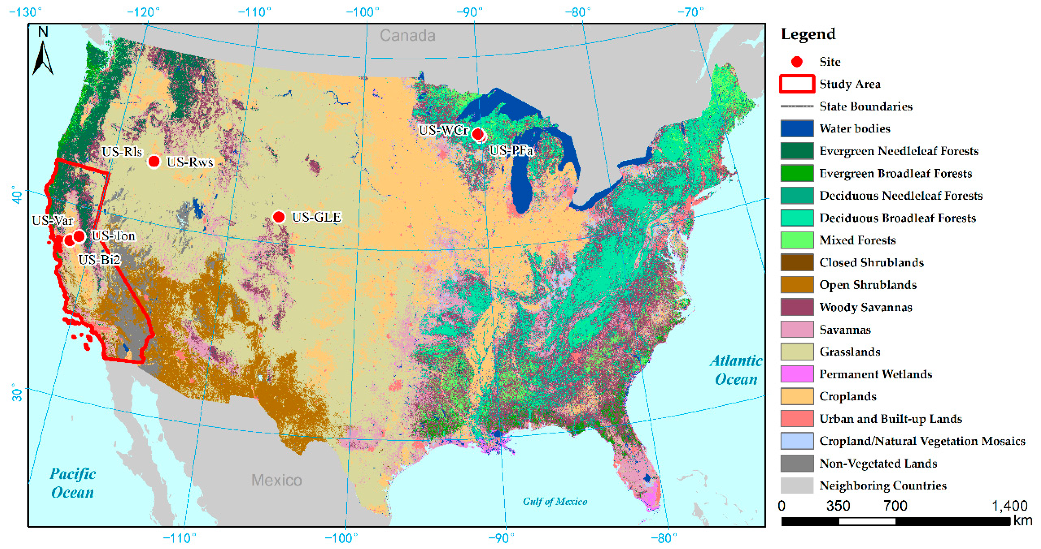
2.1. Research Sites and Region

The interest area covers regions from the upper-left corner at 45°N and −124°W to the bottom-right corner at 25°N and −89°W in North America (Figure 1). The AmeriFlux eddy covariance flux tower data were used in the study. Since the full year of available measurements by the satellite products is from 2017, we chose sites with data after 2017. The eight EC flux sites cover eight biome types, including evergreen needleleaf forests (ENF), deciduous broadleaf forests (DBF), mixed forests (MF), closed shrublands (CSH), open shrublands (OSH), woody savannas (WAS), grasslands (GRA), and croplands (CRO). Since the EC flux sites with the biome types of evergreen broadleaf forests (EBF), deciduous needleleaf forests (DNF), and savannas (SAV) are not matched in time with Sentinel-3 OLCI, this research did not estimate the GPP under these biome types at the site scale. Additionally, due to rich biome types, California was selected as the study area for regional GPP estimation.

2.2. Data

2.2.1. Sentinel-3 OLCI Land Product

Sentinel-3 OLCI is an inheritor of the Medium Resolution Imaging Spectrometer (MERIS) and has many enhancements [51,57]. There are three main kinds of OLCI products available to the public (i.e., level-1B products, level-2 land products, and level-2 water products). The level-2 land product provides land and atmospheric geophysical products at full and reduced resolution, where full resolution is approximately 300 m on the ground and reduced resolution is approximately 1200 m on the ground. An OLCI Level-2 Land Full Resolution (OL_2_LFR) product includes an OGVI band and OTCI band. OGVI describes FAPAR in the plant canopy and OTCI represents the terrestrial chlorophyll index. Sentinel-3 OLCI products applied in this study covered January 2017 to December 2018 at the US-WCr site, US-Ton site, US-PFa site and US-Var site, respectively. However, due to the lack of site data, Sentinel-3 OLCI products from January 2017 to September 2018 at the US-Rls site and US-Rws site, January 2017 to March 2018 at the US-GLE site and April 2017 to December 2018 at the US-Bi2 site were used.
The Sentinelsat module offers a powerful Python API for searching and downloading the metadata of Sentinel satellite images from the Copernicus Open Access Hub (https://scihub.copernicus.eu/dhus (accessed on 13 January 2021)) through executing condition and spatial queries (a region of interest can be created with a polygon on the GeoJSON website) and was used to batch download the OLCI online and offline products. The filtered OLCI products were automatically downloaded and stored locally as compressed files, and a total of about 5200 scene data were downloaded in this work. Then, we developed a complete set of OLCI product preprocessing processes, including mosaic, reprojection, resampling, and subset processes. The snappy module developed by the European Space Agency (ESA) and a custom script written in Python was applied to complete these data preprocessing operations. The traditional data processing software (i.e., SNAP and ENVI) either cannot batch process or takes a long time. Our python script can dramatically improve the efficiency of data processing through fully automatic data retrieval, batch processing and multithreading technology.

2.2.2. MERRA2 Daily Meteorology Reanalysis Data

Second Modern-Era Retrospective analysis for Research and Applications (MERRA2) meteorology reanalysis data with a 0.5° × 0.625° spatial resolution have been widely used in GPP modeling [5,58,59]. The data were downloaded from GMAO/NASA (https://disc.gsfc.nasa.gov (accessed on 13 January 2021)). Four MERRA2 variables were used for this study: (1) daily surface incoming shortwave flux (SWGDN, W/m2), (2) daily minimum air temperature at 2 m (T2MMIN, K), (3) daily mean air temperature at 2 m (T2MMEAN, K), and (4) relative humidity (RH, %). The SWGDN was discovered within the “Single-Level Radiation Diagnostics” collection (M2T1NXRAD), T2MMIN and T2MMEAN were found in the “Single-Level Diagnostics” collection (M2SDNXSLV), and RH was discovered within the “Assimilated Meteorological Fields” collection (M2I3NPASM).
In order to run GPP estimation models at the same spatial resolution as OLCI products, we adopted the nonlinear spatial interpolation method developed by Zhao et al. [60] for downsizing the MERRA2 meteorology reanalysis data from a 0.5° × 0.625° resolution to a 300 m OLCI pixel resolution [43,59]. This method utilizes the fourth power of the cosine function and the weighted distance in the closest four grid cell for computing the value of every output pixel with an OLCI resolution [61]. The spatial interpolation scheme may improve the meteorological input data accuracy of every 300 m pixel, eliminating sudden changes between the two sides of the MERRA2 boundary [62].

2.2.3. EC Flux Data

The EC flux data of eight AmeriFlux sites were downloaded from the AmeriFlux data portal (https://ameriflux.lbl.gov/ (accessed on 13 January 2021)). These eight AmeriFlux sites are GLEES (US-GLE), Willow Creek (US-WCr), SE5 Aspen-5 CHEESEHEAD 2019 (US-PFs), RCEW Low Sagebrush (US-Rls), Reynolds Creek Wyoming big sagebrush (US-Rws), Tonzi Ranch (US-Ton), Vaira Ranch-Ione (US-Var), and Bouldin Island corn (US-Bi2), represented by ENF, DBF, MF, CSH, OSH, WSA, GRA, and CRO, respectively (Table 1). The EC flux data have a half-hourly temporal resolution, and the daily GPP values were calculated as a sum of 30-min GPP fluxes. The REddyProc online tool (https://www.bgc-jena.mpg.de/REddyProc/brew/REddyProc.rhtml (accessed on 13 January 2021)) [63,64] implements a standardized approach for processing EC data and was used to calculate GPP for the EC flux tower when GPP was not provided. Furthermore, the online tool filters out data collection during stable atmospheric conditions using u* (friction velocity) filtering, and gap-fills missing data using a marginal distribution sampling approach. Flux measurements (net ecosystem exchange, latent heat flux and sensible heat flux) and meteorology measurements (incoming shortwave radiation, vapor pressure deficit, relative humidity, air temperature, soil temperature and friction velocity) were obtained to calculate GPP.

2.2.4. MODIS Products

The most widely used GPP product is MOD17A2H, which uses updated Biome Property look-up tables and an updated version of the daily GMAO meteorological data as input data. Since the time resolution is 8 days, there are a total of 92 scene MODIS GPP products used within two years. The purpose of using MOD17A2H is to compare of the model prediction accuracy.
The MOD12Q1 land cover product with a 500 m spatial resolution, which is one of the MODIS products, was used in the MODIS GPP algorithm. Boston University’s UMD classification scheme within the dataset was also employed for offering biome-specific information for GPP estimation models [6]. Moreover, a 1.5 km × 1.5 km area centered on every flux tower site was extracted to represent the flux footprint, the mean values of the 5 × 5 pixels and the mean values of the 3 × 3 pixels were the final GPP values for Sentinel-3 OLCI products and MODIS GPP products, respectively [5,50].

2.3. Methods

2.3.1. MODIS GPP Algorithm

Firstly, we used the MODIS GPP algorithm to estimate GPP. The MODIS GPP algorithm is applied based on the LUE model, which mainly uses the relationship between LUE and environmental factors (temperature, water vapor, and light) [28,72]. The algorithm can be expressed as follows:
GPP =   ε FAPAR IPAR
ε =   ε max TMIN _ scalar VPD _ scalar
TMIN _ scalar   =   { 0 T min < TMIN min T min TMIN min TMIN max TMIN min TMIN min < T min < TMIN max 1 T min > TMIN max
VPD _ scalar = { 0 VPD > VPD max VPD max VPD VPD max VPD min VPD min < VPD < 1 VPD < VPD min VPD max
where Ɛmax, TMINmax, TMINmin, VPDmax, and VPDmin are shown in Table 2. The biome-specific physiological parameters for each biome type are determined according to the MOD12Q1 UMD classification scheme and BPLUT (Table 3) [59]. TMIN and VPD scalars are simple linear ramp saturated at the maximum and minimum, respectively, and the range is from 0 to 1 [73]. FAPAR was obtained from the OLCI FAPAR product (OGVI). IPAR is equal to SWRad times 0.45 (Equation (1e)):
IPAR = SWRad 0.45
where SWRad, Tmin and VPD are obtained from MERRA2 meteorology reanalysis data. VPD is calculated with T2MMEAN and RH (Equation (1f)) [73]:
VPD = 610.78 e ( 17.2694 T 2 MMEAN T 2 MMEAN + 238.3 ) ( 1 RH 100 )

2.3.2. EC-LUE

Yuan et al. [32] developed the EC-LUE model which is mainly driven by FAPAR, PAR, the air temperature, and the Bowen ratio of sensible to latent heat flux. Because of the weak simulation of sensible and latent heat fluxes on a large spatial scale, adopting the Bowen ratio for presenting water stress factors (Ws) will hinder EC-LUE model application on a large scale [75]. In this study, VPD was used to replace sensible and latent heat fluxes to calculate Ws [21]. The GPP in EC-LUE is estimated as follows:
GPP = FAPAR IPAR ε max Min ( T S , W S )
where FAPAR is obtained from the OLCI FAPAR product (OGVI). IPAR is the same as in the MODIS GPP algorithm. ε max is the potential LUE without environmental stress and is set to 2.14 (gC/m2/d) [33]. Ts and Ws are the downward-regulation scalars for the individual influences of temperature and humidity on LUE. Min denotes the minimum value of Ts and Ws. Ts indicates a limiting influence of temperature on vegetation photosynthesis, based on the algorithm of the temperature limiting factor in the Terrestrial Ecosystem Model (TME) [76,77]:
T s = ( T T min ) ( T T max ) ( T T min ) ( T T max ) ( T T opt ) 2
where T is the average air temperature (°C), and Tmin, Tmax, and Topt represent the minimum, maximum, and optimum air temperatures (°C), respectively, for photosynthetic activities. If the air temperature is below Tmin or exceeds Tmax, Ts is set to zero. According to [32], this study set Tmin and Tmax to 0 and 40 °C, respectively, and Topt was determined to be 20.33 °C through nonlinear optimization. The Ws can be expressed as follows:
W s = VPD 0 VPD 0 + VPD
where VPD0 is the half-saturation coefficient of the Equation (2c), obtained from previous research (Table 4) [21].

2.3.3. The Greenness and Radiation Model (GR)

Gitelson et al. first introduced the GR model [78]. The GR model estimates GPP by adopting the chlorophyll content, as well as incoming solar radiation. This model was successfully applied within irrigated and rainfed maize, wheat cropland, and forest [48]. The GR model can be expressed as follows:
GPP = Chl IPAR m
where Chl was replaced with OTCI in this study. The parameter m is a scalar decided by the model calibration. The calculation method of model calibration is described in Section 2.3.5.

2.3.4. The Vegetation Index Model (VI)

The VI model employed for GPP estimation was proposed by Wu et al. and applied in crop and deciduous forest ecosystems [42]. It assumes that the VIs are a reliable proxy of both LUE and FAPAR, so the product VIs ∗ VIs ∗ IPAR is used to estimate GPP. In this paper, VIs is same, so the VI model can be expressed as:
GPP = VIs 2 IPAR m
where OTCI is regarded as the VI parameter of the model input, m is the same as in the GR model.

2.3.5. Calibration of the GR and VI Model

Model calibration is an important step for the operational application of the GR and VI models and greatly impacts model accuracy [48,79]. GR and VI model calibration mainly involves the calculation of scalar m. At present, calibration methods can be divided into adopting the half-data method (the rest of the data are used for model validation) [23] and the all-data method (all data are applied to model calibration and validation) [46,48]. In this work, to conduct a rigorous test of the model, we chose half-data to calibrate the model. The rest of the data were then applied when testing the model. The values of scalar m were obtained through establishing a directly linear relationship between in situ measured GPP and model-estimated GPP values, and scalar m is the slope of linear function.

2.3.6. Analytical Methods

Three statistic analytical indices can be adopted for evaluating the accuracies and uncertainties of all GPP models: (1) the coefficient of determination (R2), which expresses the fit between model prediction results and true values; (2) the root mean square error (RMSE), which refers to sample standard deviation between predictions and measurements; and (3) bias, which reflects the differences between the estimates and the observation. RMSE and bias are calculated as follows:
RMSE = 1 n i = 1 n ( M i E i ) 2
Bias = 1 n i = 1 n ( M i E i )
where Mi and Ei are the predicted GPP and measured GPP values, respectively. Notably, in subsequent chapters, GPPEC represents the on-site measured GPP values, and GPPMOD17 represents the GPP values from MODIS-GPP products. GPPMODIS-GPP, GPPEC-LUE, GPPGR, and GPPVI represent GPP estimation values obtained from the MODIS-GPP algorithm, EC-LUE model, GR model, and VI model, respectively.

3. Results

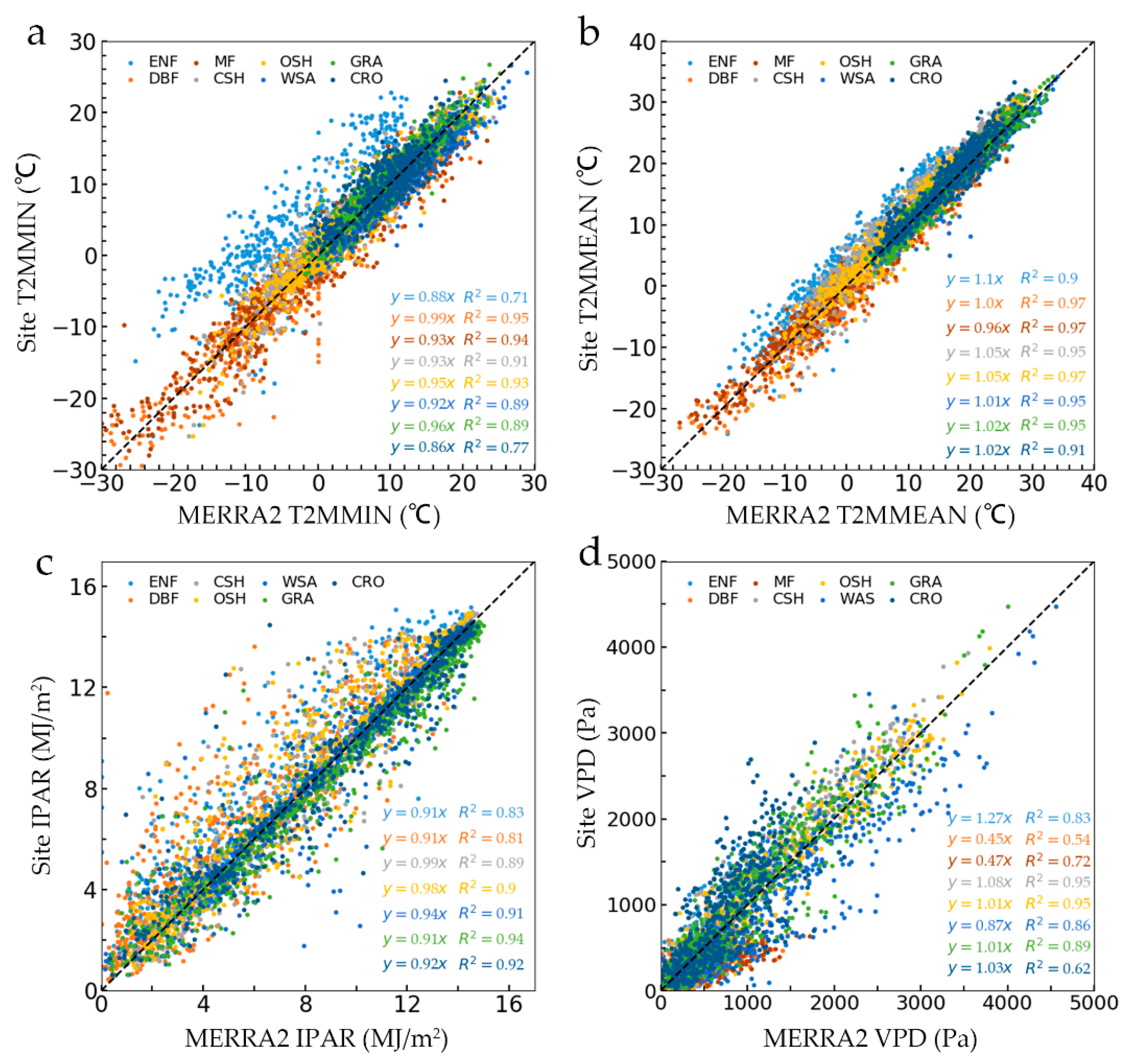
3.1. Meteorology Variables

In this study, the MERRA2 meteorology reanalysis data were taken as site meteorological data for four GPP estimation models. For determining the meteorological data effects on GPP estimation, we conducted a direct comparison of daily MERRA2 meteorology reanalysis data and site meteorological data (Figure 2). The two datasets have a strong correlation with T2M_MIN and T2M_MEAN (Figure 2a,b), suggesting that the MERRA2 meteorology reanalysis data can be reliably applied to estimate the on-site temperature conditions. The IPAR (Figure 2c) at the eight sites had a high correlation with the measured data. The R2 was above 0.8, and the scatter distribution was very close to the 1:1 line, which indicated that the on-site IPAR could be reliably calculated from the MERRA2 meteorology reanalysis data. For VPD (Figure 2d), R2 varied at different sites, and the range of R2 was 0.51–0.95. Among them, VPD at the US-WCr (DBF) and US-Bi2 (CRO) obtained a relatively low accuracy, with R2 = 0.54 and 0.62, respectively. The VPD across shrublands obtained the highest accuracy (R2 = 0.95).

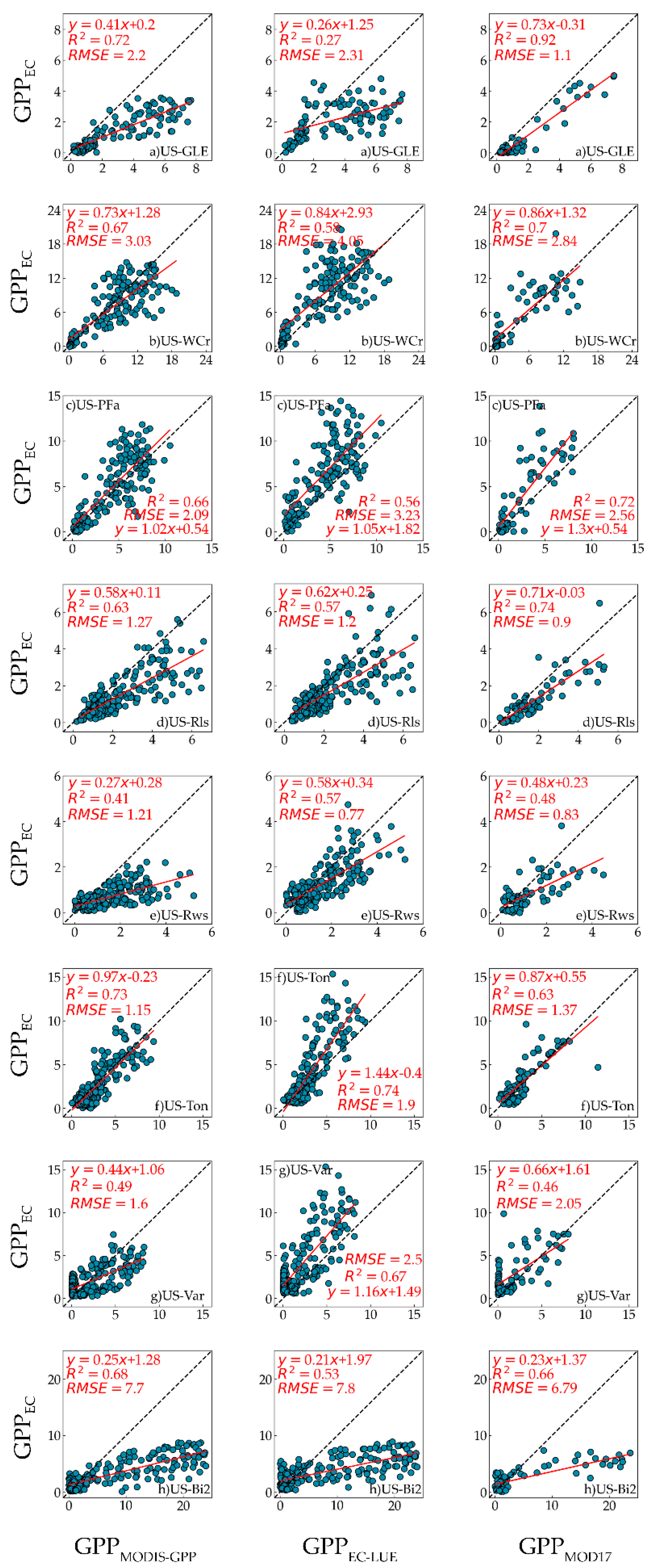
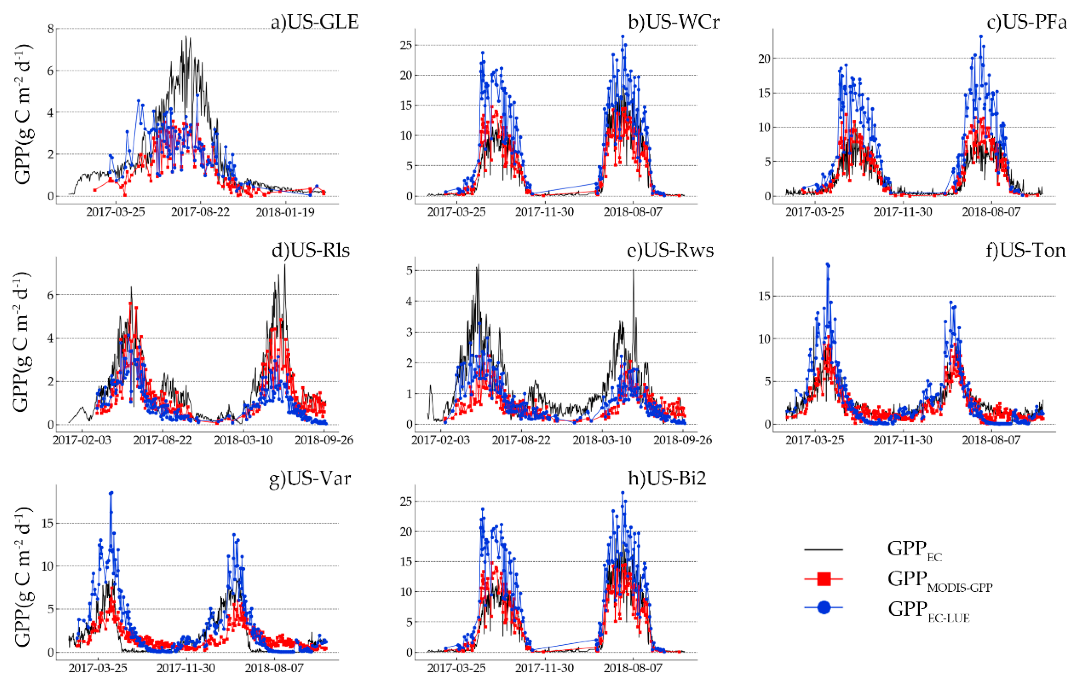
3.2. Agreement between GPPMODIS-GPP, GPPEC-LUE, GPPMOD17 and GPPEC

We first compared the performance of GPPMODIS-GPP and GPPEC-LUE against that of the GPPEC at all sites for 2017 and 2018 (Figure 3). For the MODIS-GPP algorithm, the results showed that the US-Ton site obtained the best performance (R2 = 0.73), followed by US-GLE with R2 = 0.72, US-Bi2 with R2 = 0.68, US-WCr with R2 = 0.67, US-PFa with R2 = 0.66, and US-Rls with R2 = 0.63 (Table 5). The R2 values between the GPPMODIS-GPP and GPPEC at the US-Var site and US-Rws site were lower than 0.5. In terms of the RMSE, the US-Bi2 site produced the maximum error (RMSE = 7.70 gC/m2/d) and the US-Ton site displayed the lowest error with RMSE = 1.15 gC/m2/d.
For the EC-LUE model, the results showed that the US-Ton site obtained the best performance (R2 = 0.74), followed by the US-Var with R2 = 0.67, US-WCr with R2 = 0.58, US-Rws with R2 = 0.57, US-PFa with R2 = 0.57, US-PFa with R2 = 0.56, and US-Bi2 with R2 = 0.53. However, insignificant correlations were obtained at the US-GLE site, and this situation was mainly influenced by the ENF when using EC-LUE model [32,75]. For MODIS-GPP products, the US-GLE site exhibited the best performance, with R2 = 0.92. At the US-Rws site and US-Var site, GPPMOD17 performed relatively poorly, with R2 = 0.48 and 0.46, respectively. These results were consistent with GPPMODIS-GPP. It is worth noting that the performance of GPPMOD17 was worse than GPPMODIS-GPP for the US-Ton, US-Var, and US-Bi2 site and worse than GPPEC-LUE for the US-Rws, US-Ton, and US-Var site.
Figure 4 illustrates the temporal variation of GPPMODIS-GPP, GPPEC-LUE and GPPEC for all sites. Overall, GPPMODIS-GPP and GPPEC-LUE effectively matched GPPEC and generally captured the seasonal variations aligned with the GPPEC. As shown in Table 5, GPPMODIS-GPP tracked GPPEC well at the US-Ton site, with the lowest RMSE (1.14 gC/m2/d) and the second-lowest bias (−0.30 gC/m2/d). Similarly, GPPEC-LUE tracked GPPEC well at the US-Rws site, with the lowest RMSE (1.01 gC/m2/d) and bias (−0.72 gC/m2/d). However, there were still substantial underestimations and overestimations in some sites among GPPMODIS-GPP, GPPEC-LUE and GPPEC. For example, for the MODIS-GPP algorithm, at the US-Bi2 site, GPPMODIS-GPP were underestimated (RMSE = 7.70 gC/m2/d, bias = −4.53 gC/m2/d). For the EC-LUE model, GPP fluxes were underestimated at several sites, such as the US-Bi2 site (RMSE = 7.80 gC/m2/d, bias = −4.15 gC/m2/d) and the US-GLE site (RMSE = 2.31 gC/m2/d, bias = −1.39 gC/m2/d), but GPPEC-LUE values at the US-PFa site (RMSE = 3.23 gC/m2/d, bias = 2.07 gC/m2/d) and the US-WCr site (RMSE = 4.05 gC/m2/d, bias = 1.71 gC/m2/d) were overestimated. Notably, GPPMODIS-GPP at the US-WCr site and GPPEC-LUE at the US-Ton site obtained a low bias but high RMSE. It was because the underestimation of GPP offset part of the deviation during the months of 2017, as well as the overestimation of compensation in 2018 or GPP underestimation during the growing season, alongside overestimation during the nongrowing season.

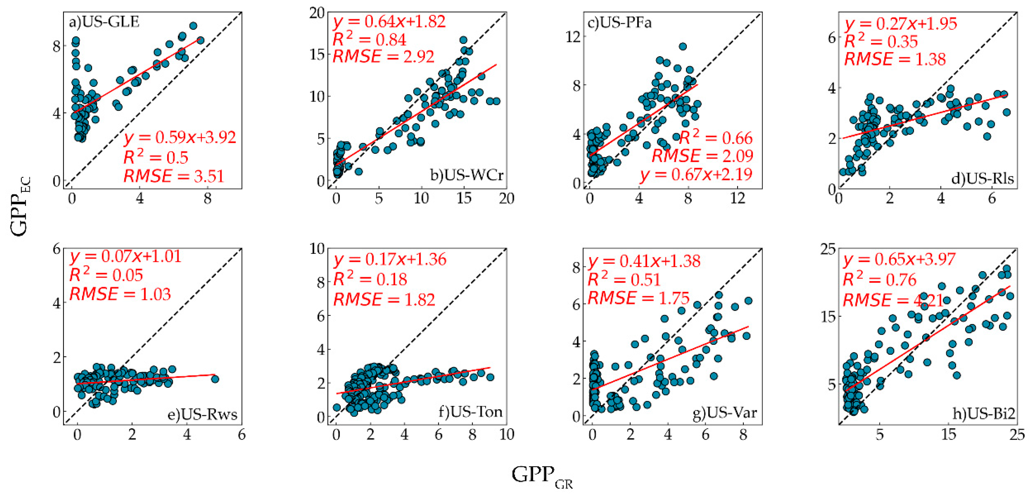
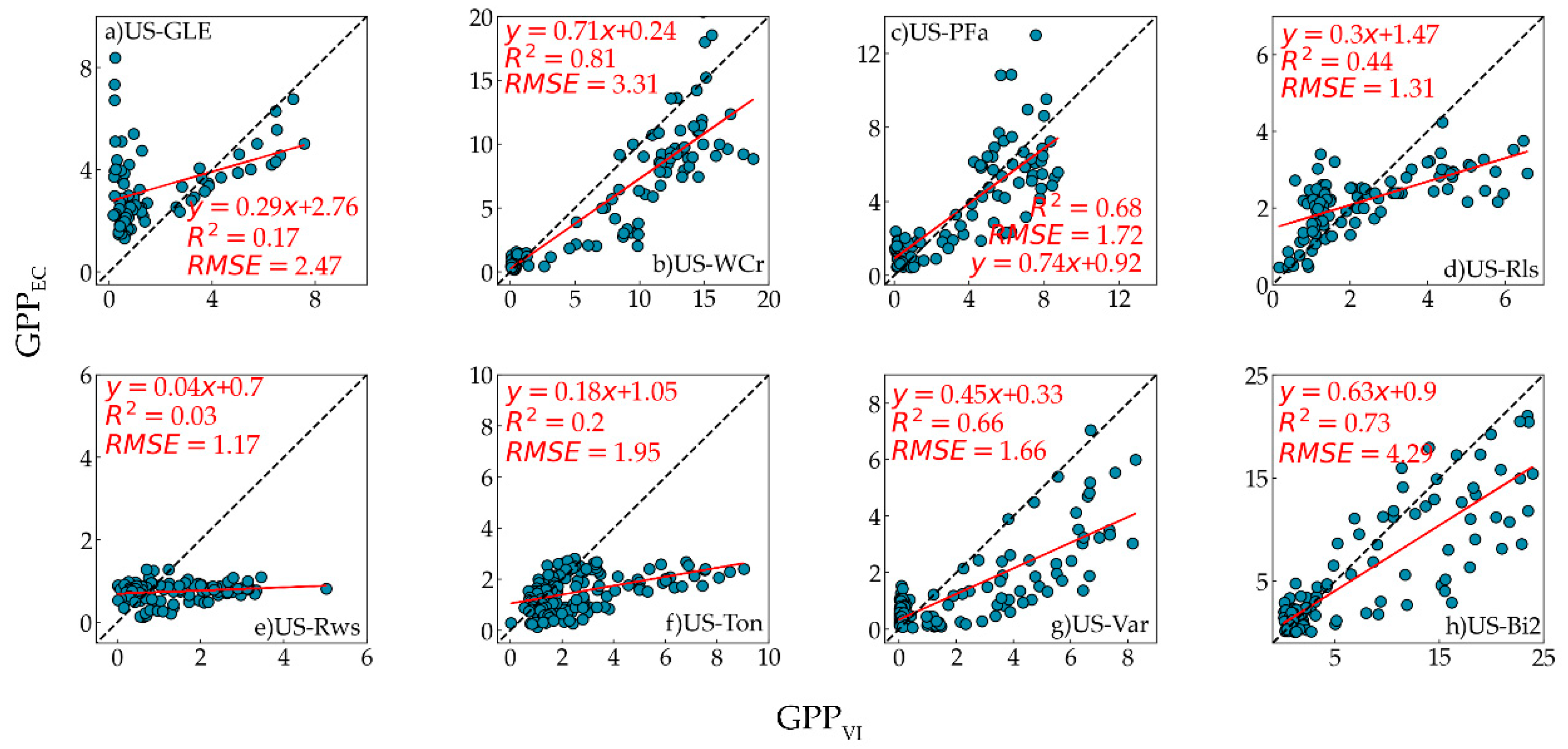
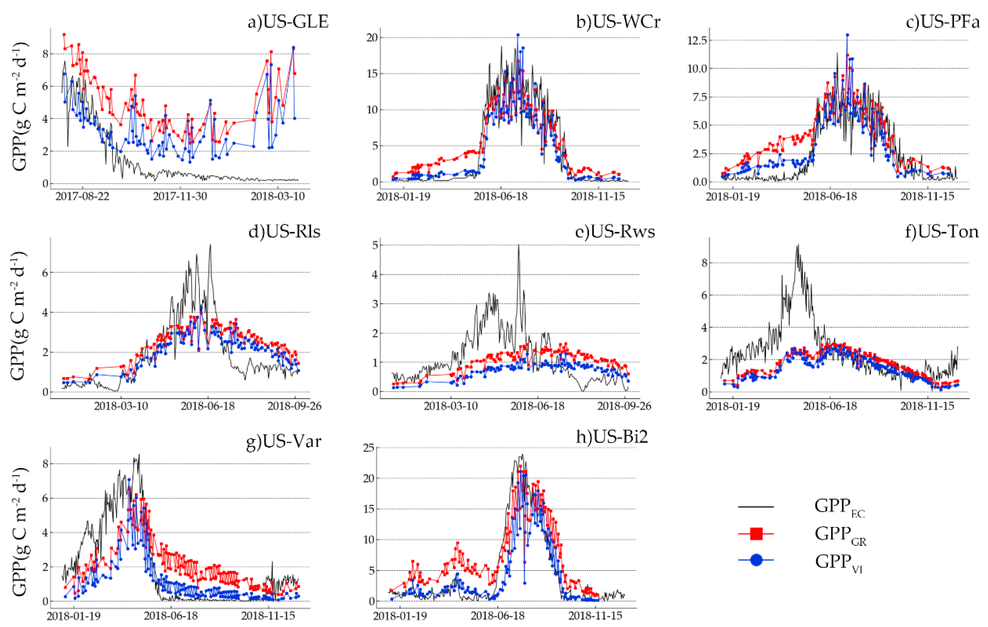
3.3. Agreement between GPPGR, GPPVI and GPPEC

The scatter plots between the GPPGR, GPPVI, and GPPEC for every site are displayed in Figure 5 and Figure 6. The performance of the two models is different at various sites. Therefore, the two models’ applicability depends on the biome type. For example, insignificant correlations between the GR and VI models were obtained at the US-Rws site, US-Ton site and US-Rls site. Even for the same biome type, their performance was different. For instance, the GR model had a better performance than the VI model at the US-GLE site. Additionally, strong relationships between GPPGR, GPPVI and GPPEC were established at the US-WCr site, US-Bi2 site, US-PFa site, and US-Var site. In particular, the GR and VI models both obtained the best performance at the US-WCr site, with R2 = 0.84 and 0.81, respectively.
The time series of GPPGR, GPPVI and GPPEC in 2017–2018 are presented in Figure 7. Overall, the temporal dynamics of GPPGR and GPPVI are roughly the same. The GPPGR and GPPVI tracked the GPPEC well at the US-Bi2 site, US-PFa site, US-Var site, and US-WCr site. As shown in Table 6, GPPGR and GPPVI at the US-GLE site were overestimated, with bias = 3.18 gC/m2/d and 1.16 gC/m2/d, respectively. Additionally, GPPGR and GPPVI were underestimated at the US-Ton site, with bias = −0.75 gC/m2/d and −1.48 gC/m2/d, respectively. Notably, both GPPGR and GPPVI showed a poor relationship with GPPEC at the US-Rls site and US-Rws site. This situation was mainly due to the underestimated GPP values during the growing season and overestimating GPP values during the nongrowing season.

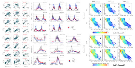
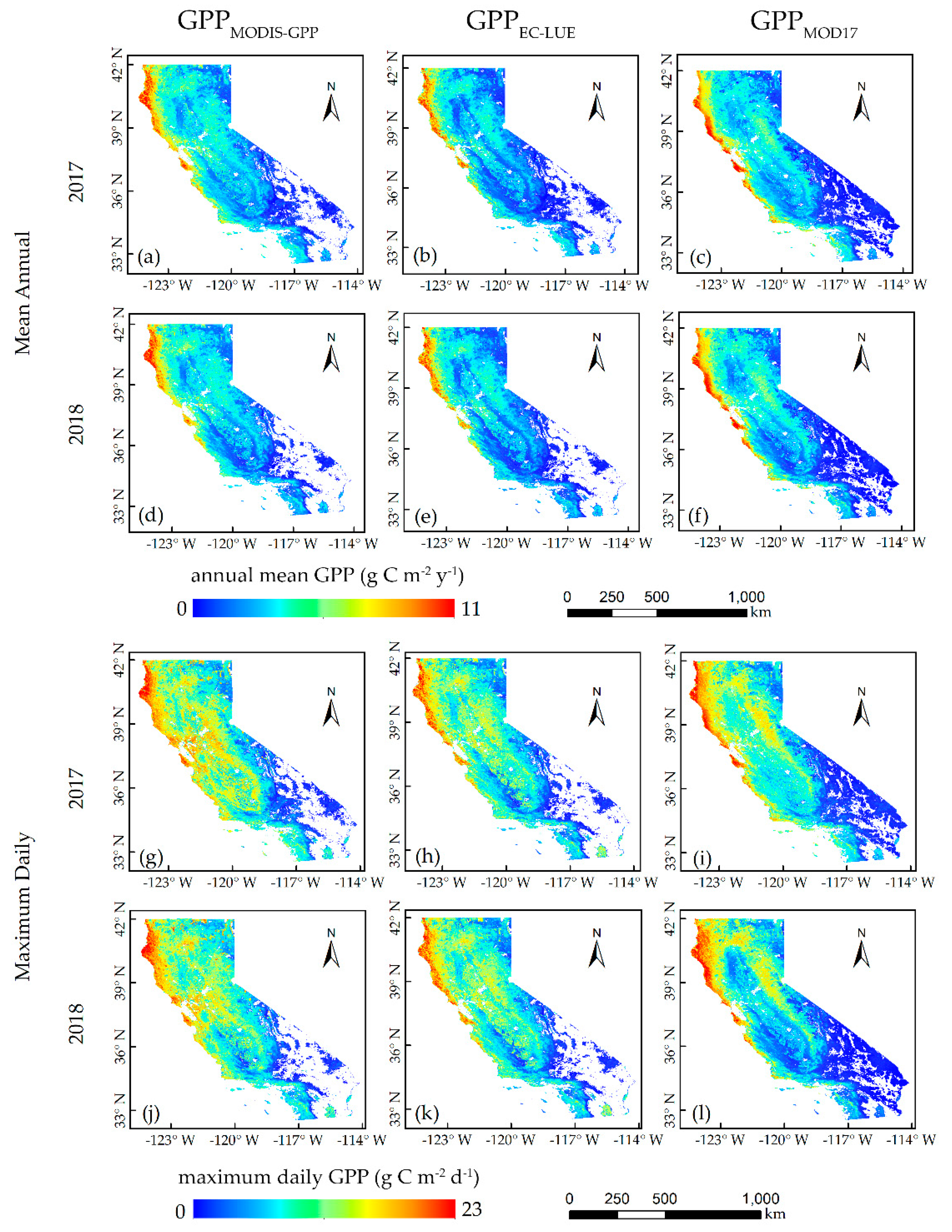
3.4. Spatial−Temporal Consistency between GPPMODIS-GPP, GPPEC-LUE and GPPMOD17

We compared the spatial distribution of the annual mean GPP (gC/m2/d) and maximum daily GPP (gC/m2/d) from GPPMODIS-GPP and GPPEC-LUE across California in North America during 2017 and 2018 at a 300 m spatial resolution. The annual mean GPP was the average of each pixel throughout the year. The maximum daily GPP was the maximum value of each pixel throughout the year. Notably, the spatial distributions of GPPGR and GPPVI were not shown here due to the insufficient calibration data for upscaling to the regional scale. Figure 8a−f show the spatial distribution of the annual mean GPP throughout California. The GPPMODIS-GPP and GPPEC-LUE reached the highest values in the western coastal area and decreased along a longitudinal gradient from the west (dominated by forest) to the east (dominated by shrubland and grassland). For the maximum daily GPP (Figure 8g−l), the highest value was ~23 gC/m2/d for the Northwest Coastal Forest Belt. The southeastern shrubland region had low GPP values. From 2017 to 2018, the maximum daily GPP decreased significantly in the southwestern shrubland (35°N–37°N, −121°W–199°W). The biggest discrepancy between the annual mean GPP value and maximum daily GPP value could be found in the central croplands, where the maximum daily GPP was high, and the annual mean GPP was moderate. Overall, the GPPMODIS-GPP and GPPEC-LUE showed similar spatial−temporal patterns to GPPMOD17. Notably, compared with GPPMOD17, GPPMODIS-GPP, and GPPEC-LUE relatively underestimated the GPP values for cropland.

4. Discussion

The R2 between GPPMODIS-GPP, GPPEC-LUE, and GPPEC showed the strong correlation between modelled GPP and measured GPP. The performance of RMSE varied at different sites. Compared with GPPMOD17, GPPMODIS-GPP offered better GPP prediction at the US-Ton site and US-Bi2 site, and GPPEC-LUE offered better GPP prediction at the US-Ton site, US-Var site, and US-Rws site. At the US-Ton site, GPPMODIS-GPP and GPPEC-LUE obtained the best performance. Previous research showed that the savanna GPP estimation accuracy was smaller than other biome types because of the misclassification and sparse vegetation cover [50,74,80]. However, the woody savanna has a denser vegetation cover than the savanna [74,80,81]. This structure can reduce the influence of understory vegetation and improve GPP estimation accuracy [82]. Additionally, GPPMODIS-GPP and GPPEC-LUE also obtained a good performance at the US-WCr site and US-PFa site. This finding was consistent with previous studies [5,83]. For the US-WCr site, both GPPMODIS-GPP and GPPEC-LUE performed best in estimating GPP. The reasons for this can be summarized as follows. Firstly, DBF has obvious seasonal and phenological characteristics which can be monitored by satellites in real time [32]. Secondly, the vegetation structure of DBF is simple and the vegetation coverage varies greatly in different seasons, so the estimation of FAPAR is relatively simple and accurate [32]. Thirdly, DBF usually grows at mid and high latitudes with less cloudiness so that high-quality time-series images can be obtained [44]. For the US-PFa site, GPPMODIS-GPP and GPPEC-LUE represented the growth status of MF. However, compared with GPPMODIS-GPP, GPPEC-LUE was overestimated (RMSE = 3.23 gC/m2/d, bias = 2.07 gC/m2/d). The factor that caused this overestimation was the complex vegetation structure of the mixed forest, which had various Ɛmax due to abundant plant species. Moreover, the leaf shape, tree height, and light energy absorption conditions are different among tree species. Therefore, a single Ɛmax used in the input model causes certain errors [84,85]. The performance of GPPMODIS-GPP and GPPEC-LUE at two shrubland sites varied. For the US-Rls site, GPPMODIS-GPP and GPPEC-LUE both had a moderate correlation against GPPEC, with R2 = 0.63 and 0.57, respectively. However, for the US-Rws site, the accuracy of GPPMODIS-GPP was the lowest, and the performance of GPPEC-LUE was better than that of GPPMODIS-GPP. The factor that caused this phenomenon was the estimation accuracy of GPP at shrubland sites, which varied in different areas [22,86]. The growth of shrubland is mainly affected by water, so more consideration should be given to water influence factors when estimating shrubland GPP [81,84]. Therefore, for shrubland in temperate and frigid zones, GPP estimation accuracy is higher, but in the tropics, affected by VPD and FAPAR, the accuracy of shrubland GPP estimation is lower. At the US-Var site, the performance of GPPEC-LUE was also better than GPPMODIS-GPP, and the accuracy of the GPPEC-LUE was the second highest (R2 = 0.67). The accuracy of GPPMODIS-GPP (R2 = 0.49) was consistent with that of GPPMOD17 (R2 = 0.46). However, the performance of GPPMODIS-GPP at the US-GLE site was far better than that of GPPEC-LUE. For the US-GLE site, the accuracy of GPPMODIS-GPP was worse than the US-Ton site (R2 = 0.72). For the US-Bi2 site, the relationship between GPPMODIS-GPP, GPPEC-LUE and GPPEC was moderate, and GPPMODIS-GPP and GPPEC-LUE obviously underestimated the cropland GPP (RMSE = 7.70 gC/m2/d, bias = −4.53 gC/m2/d and RMSE = 7.80 gC/m2/d, Bias = −4.15 gC/m2/d, respectively). This finding is aligned with previous research [50,87]. In crop ecosystems, different crops have different Ɛmax and growth cycles, so a single Ɛmax cannot represent well all types of crops [88,89]. Additionally, the rotation period varies for different crop types. Therefore, if the same input variables are used to estimate GPP for different crops, this can lead to a large deviation in GPP estimation [90].
The performance of GPPGR and GPPVI was diverse for different biome types. The correlation between GPPGR, GPPVI, and GPPEC was strongest at the US-WCr site, with R2 = 0.84 and 0.81, respectively. Compared to the US-WCr site, the correlation between GPPGR, GPPVI and GPPEC was relatively weak at the US-GLE site. This result was consistent with previous research, where OTCI was highly correlated with tower GPP across deciduous forests and weakly correlated with tower GPP across evergreen forests [49,50]. The reason for this phenomenon could be that stress causes a decrease of the photosynthetic efficiency [91], the conical canopy structure, and the density of evergreen needleleaf trees. The consequent shadowing effect leads to the failure of OTCI for detecting subtle changes within the seasonal chlorophyll content of evergreen needleleaf forests [92,93]. Additionally, GPPGR and GPPVI showed moderate correlations with GPPEC at the US-PFa site. The factors that caused this can be considered from two aspects. Firstly, the vegetation structure of mixed forests is complex, and different vegetation types will affect the estimation of GPP. Secondly, mixed forest productivity will drop sharply when the temperature drops in a short period. However, the vegetation index cannot change significantly in this case, leading to its failure in capturing the impact of temperature change on GPP [47,94,95]. A strong correlation could also be observed between GPPGR, GPPVI, and GPPEC at the US-Bi2 site. Previous studies have found a similar relationship between OTCI or other chlorophyll indices and GPP [49,78,96]. Notably, GPPGR and GPPVI had the highest RMSE (4.21 gC/m2/d and 4.29 gC/m2/d, respectively) at the US-Bi2 site. The reason for this is that compared with GPPEC, GPPGR and GPPVI overestimated GPP in the nongrowing season and underestimated it in the growing season (Figure 7h). A previous study demonstrated that OTCI started to increase earlier than the time of corn sowing [49]. The high GPPGR and GPPVI obtained in the nongrowing season may represent fallow land, which is gradually colonized by weed species or affected by humidity changes, and not represent actual crop growth [49]. At the US-Var site, the correlation between GPPVI and GPPEC (R2 = 0.66) was better than that between GPPGR and GPPEC (R2 = 0.50). This difference may be related to the vertical and horizontal heterogeneity of grasslands [49]. C3 annual grasses dominated the US-Var site. Previous studies [49,97] showed that, compared with grasslands dominated by C4 species, C3 grasslands exhibited lower OTCI values during the peak growth period, explaining why GPPVI had a higher accuracy than GPPGR. However, GPPGR and GPPVI performed poorly in woody savannas and two shrubland sites. The probable reason for this was that the influence of the soil background on the low vegetation coverage at these sites led to the failure of OTCI in tracking GPP [50].
At the regional scale, GPPMODIS-GPP and GPPEC-LUE agreed quite well with GPPMOD17. For the annual mean GPP, GPPMODIS-GPP and GPPEC-LUE were relatively high in the western coastal areas, where the biome types were mainly evergreen forests. The low GPPMODIS-GPP and GPPEC-LUE were obtained in grasslands. The finding aligned with a previous study [61], where evergreen forests exhibited strong photosynthesis and open shrublands were the least productive. Forest ecosystems have a relatively higher maximum daily GPP, and open shrublands have the lowest maximum daily GPP compared with other vegetation types. Notably, the maximum daily GPP across grasslands in the northeast was larger than in central areas, and the high sensitivity to soil moisture may be the cause of this phenomenon [61]. The inconsistency between the annual mean GPP and maximum daily GPP may be mostly due to the influence of temperature and rainfall on the length of the different growing seasons [61].
In addition, we further analyzed the uncertainty in simulating GPP using Sentinel-3 OLCI products and MERRA2 meteorology reanalysis data in this study. Several factors can influence the GPP estimation using the MODIS-GPP algorithm and EC-LUE model. First is the inconsistency of the spatial resolution between Sentinel-3 and meteorology reanalysis data. The errors may have been derived from the interpolation of MERRA2 meteorology reanalysis data from 0.5° × 0.625° to 300 m. Second is the coarse classification of vegetation types on land cover maps. Boston University’s UMD classification scheme in the MOD12Q1 land cover dataset classifies croplands as one category and does not distinguish between C3 and C4 crops. C3 and C4 crops possess various photosynthetic pathways and light use efficiencies [88,89]. Because the C3/C4 mixing ratio for each cropland pixel is unknown, we simply used the single Ɛmax and meteorological parameters to estimate GPP on a large scale. Therefore, GPPMODIS-GPP and GPPEC-LUE are underestimated or overestimated in croplands. Thirdly, the image data quality is also a significant factor influencing GPP estimation. Due to atmospheric contamination (i.e., clouds, aerosols), Sentinel-3 OLCI products have more missing data and low reliability during winter. Future work should be focused on spatial−temporal fusion techniques, which can further enhance the temporal and spatial continuity of Sentinel-3 OLCI products by fusing Sentinel-2 images with Sentinel-3 OLCI to achieve more accurate regional and large-scale GPP estimation [98,99].
Although our results showed that GPPMODIS-GPP, GPPEC-LUE, GPPGR and GPPVI did not always perform better than GPPEC or GPPMOD17, it needs to be emphasized that the objective of our study was not to distinguish which model was superior for GPP estimation. Our study aimed to demonstrate the potential of integrating Sentinel-3 OLCI products and MERRA2 meteorology reanalysis data to estimate GPP at site and regional scales. Our results also demonstrated that the LUE model and VI-driven model were suitable for ESA’s Sentinel-3 data. The Sentinel-3 Sea and Land Surface Temperature Radiometer (SLSTR) provides land surface temperature (LST) products with a higher temporal resolution. In future research, the integration of SLSTR LST products and OLCI FAPAR or meteorology reanalysis data in other models for estimating GPP should be conducted. For a wider application of Sentinel-3 OTCI products, future work requires more in situ data to explore the OTCI and GPP’s relationship. Moreover, further investigations should focus on combining other remote sensing data or satellite-driven models with OTCI-based models. Previous studies have found that meteorological factors could improve VI-driven GPP estimation models [23]. Some existing satellite-driven models could make up for the insufficiency of GPP models based on physiologically driven spectral indices, such as MTCI [100,101]. Additionally, the Fluorescence Explorer satellite, the ESA’s eighth Earth Explorer, is expected to be launched by 2022, which can offer important auxiliary data for using Sentinel-3 products to estimate GPP [33,102].

5. Conclusions

Within this research, we assessed the performance of two Sentinel-3 OLCI products (FAPAR and OTCI) combined with MERRA2 meteorology reanalysis data to estimate GPP through four GPP models (the MODIS GPP algorithm, EC-LUE model, GR model, and VI model) at the site and regional scales during 2017 and 2018. The following major conclusions can be drawn from the study:
(1) The relationship between GPPMODIS-GPP, GPPEC-LUE and GPPEC is obvious for all sites. GPPMODIS-GPP exhibited the best performance with GPPEC at the US-Ton site (R2 = 0.73), and the weakest performance for the US-Rws site (R2 = 0.41). In addition, GPPMODIS-GPP and GPPEC-LUE were underestimated or overestimated at several sites, such as the US-Bi2 site, US-GLE site, US-WCr site and US-PFa site. Compared with GPPMOD17, GPPMODIS-GPP was superior to GPPEC at the US-Ton site, US-Var site, and US-Bi2 site, and GPPEC-LUE was superior at the US-Ton site, and the US-Var site;
(2) Compared with GPPEC, the performance of GPPGR and GPPVI varied across different biome types. Good performances were obtained across deciduous broadleaf forests, mixed forests, grasslands, and croplands, and low R2 values were obtained across evergreen needleleaf forests, shrublands, and woody savannas;
(3) At the regional scale, GPPMODIS-GPP and GPPEC-LUE both showed a very high spatial−temporal consistency with GPPMOD17. The GPP value was high in the western coastal area and low in southwestern shrubland across California. The annual mean GPP value and maximum daily GPP exhibited a strong correlation with GPPMOD17 in broadleaf forests, mixed forests, grasslands and croplands, but a relatively weak correlation in evergreen needleleaf forests and shrublands.

Author Contributions

Conceptualization, F.Z.; methodology, F.Z.; software, F.Z.; validation, F.Z. and Z.Z.; formal analysis, F.Z.; investigation, F.Z. and Z.Z.; resources, F.Z.; data curation, F.Z.; writing—original draft preparation, F.Z.; writing—review and editing, Z.Z. and L.Z.; visualization, F.Z.; supervision, Y.L. and L.Z.; project administration, F.Z. and Z.Z.; funding acquisition, Y.L. and L.Z. All authors have read and agreed to the published version of the manuscript.

Funding

This research was funded by the National Key Research and Development Program of China (2017YFB0503500), the National Natural Science Foundation of China (41930104), and the Natural Science Foundation of Jiangsu Province (SBK2019022628).

Institutional Review Board Statement

Not applicable.

Informed Consent Statement

Not applicable.

Data Availability Statement

Data sharing is not applicable to this article.

Acknowledgments

The authors would like to thank the AmeriFlux community for the eddy covariance data they provided for free, as well as the science team members who produce and manage the MODIS, MERRA2 meteorology reanalysis data and Sentinel-3 data.

Conflicts of Interest

The authors declare no conflict of interest.

Abbreviations

GPPGross primary production
LUELight use efficiency
VIsVegetation indices
ECEddy covariance
MODISModerate resolution imaging spectroradiometer
MTCIMERIS Terrestrial Chlorophyll Index
OLCIOcean and Land Colour Instrument
OTCIOLCI Terrestrial Chlorophyll Index
GRGreenness and radiation model
TGTemperature and greenness model
MOD17MODIS GPP products
GPPMODIS-GPPGPP values obtained from MODIS-GPP algorithm
GPPEC-LUEGPP values obtained from EC-LUE model
GPPGRGPP values obtained from GR model
GPPVIGPP values obtained from VI model
GPPECGPP values obtained from eddy covariance flux towers
GPPMOD17GPP values obtained from MODIS-GPP products
FAPARFraction of absorbed photosynthetically active radiation
APARAbsorbed photosynthetically active radiation
IPARIncident photosynthetically active radiation
T2MMINMinimum air temperature at 2 m
T2MMEANMean air temperature at 2 m
RHRelative humidity
SWRadSurface incoming shortwave flux
VPDVapor pressure deficit
WSWater stress factors
TSTemperature stress factors
TAverage air temperature
TminMinimum air temperature
TmaxMaximum air temperature
ToptOptimum air temperature
ƐmaxMaximum light use efficiency
ChlChlorophyll content
LSTLand surface temperature
EVIEnhanced vegetation index

References

  1. Zhang, Y.; Xiao, X.; Wu, X.; Zhou, S.; Zhang, G.; Qin, Y.; Dong, J. A global moderate resolution dataset of gross primary production of vegetation for 2000–2016. Sci. Data 2017, 4, 170165. [Google Scholar] [CrossRef] [PubMed] [Green Version]
  2. Beer, C.; Reichstein, M.; Tomelleri, E.; Ciais, P.; Jung, M.; Carvalhais, N.; Rödenbeck, C.; Arain, M.A.; Baldocchi, D.; Bonan, G.B.; et al. Terrestrial gross carbon dioxide uptake: Global distribution and covariation with climate. Science 2010, 329, 834–838. [Google Scholar] [CrossRef] [Green Version]
  3. Chapin, F.S.; Matson, P.A.; Vitousek, P.M. Principles of Terrestrial Ecosystem Ecology; Springer: New York, NY, USA, 2011. [Google Scholar]
  4. Badgley, G.; Anderegg, L.D.L.; Berry, J.A.; Field, C.B. Terrestrial gross primary production: Using NIRV to scale from site to globe. Global Chang. Biol. 2019, 25, 3731–3740. [Google Scholar] [CrossRef] [PubMed]
  5. Wu, C.; Munger, J.W.; Niu, Z.; Kuang, D. Comparison of multiple models for estimating gross primary production using MODIS and eddy covariance data in Harvard Forest. Remote Sens. Environ. 2010, 114, 2925–2939. [Google Scholar] [CrossRef]
  6. Xiao, J.; Zhuang, Q.; Baldocchi, D.D.; Law, B.E.; Richardson, A.D.; Chen, J.; Oren, R.; Starr, G.; Noormets, A.; Ma, S.; et al. Estimation of net ecosystem carbon exchange for the conterminous United States by combining MODIS and AmeriFlux data. Agric. For. Meteorol. 2008, 148, 1827–1847. [Google Scholar] [CrossRef] [Green Version]
  7. Baldocchi, D. Flux Footprints Within and Over Forest Canopies. Bound. Layer Meteorol. 1997, 85, 273–292. [Google Scholar] [CrossRef]
  8. Schmid, H.P. Source areas for scalars and scalar fluxes. Bound. Layer Meteorol. 1994, 67, 293–318. [Google Scholar] [CrossRef]
  9. Ruimy, A.; Saugier, B.; Dedieu, G. Methodology for the estimation of terrestrial net primary production from re-motely sensed data. J. Geophys. Res. Atmos. 1994, 9, 5263–5283. [Google Scholar] [CrossRef]
  10. Lieth, H. Modeling the Primary Productivity of the World. In Primary Productivity of the Biosphere; Lieth, H., Whittaker, R.H., Eds.; Springer: Berlin/Heidelberg, Germany, 1975; pp. 237–263. [Google Scholar]
  11. Box, E. Quantitative Evaluation of Global Primary Productivity Models Generated by Computers. In Primary Productivity of the Biosphere; Lieth, H., Whittaker, R.H., Eds.; Springer: Berlin/Heidelberg, Germany, 1975; pp. 265–283. [Google Scholar]
  12. Uchijima, Z.; Seino, H. Agroclimatic Evaluation of Net Primary Productivity of Natural Vegetations. (1) Chikugo Model for Evaluating Net Primary Productivity. J. Agric. Meteorol. 1985, 40, 343–352. [Google Scholar] [CrossRef]
  13. Jung, M.; Reichstein, M.; Margolis, H.A.; Cescatti, A.; Richardson, A.D.; Arain, M.A.; Arneth, A.; Bernhofer, C.; Bonal, D.; Chen, J.; et al. Global patterns of land-atmosphere fluxes of carbon dioxide, latent heat, and sensible heat derived from eddy covariance, satellite, and meteorological observations. J. Geophys. Res. Biogeosci. 2011, 116. [Google Scholar] [CrossRef] [Green Version]
  14. Foley, J.A.; Prentice, I.C.; Ramankutty, N.; Levis, S.; Pollard, D.; Sitch, S.; Haxeltine, A. An integrated biosphere model of land surface processes, terrestrial carbon balance, and vegetation dynamics. Glob. Biogeochem. Cycles 1996, 10, 603–628. [Google Scholar] [CrossRef]
  15. Sitch, S.; Smith, B.; Prentice, I.C.; Arneth, A.; Bondeau, A.; Cramer, W.; Kaplan, J.O.; Levis, S.; Lucht, W.; Sykes, M.T.; et al. Evaluation of ecosystem dynamics, plant geography and terrestrial carbon cycling in the LPJ dynamic global vegetation model. Glob. Chang. Biol. 2003, 9, 161–185. [Google Scholar] [CrossRef]
  16. Friend, A.D.; Stevens, A.K.; Knox, R.G.; Cannell, M.G.R. A process-based, terrestrial biosphere model of ecosystem dynamics (Hybrid v3.0). Ecol. Model. 1997, 95, 249–287. [Google Scholar] [CrossRef]
  17. Cramer, W.; Kicklighter, D.W.; Bondeau, A.; Iii, B.M.; Churkina, G.; Nemry, B.; Ruimy, A.; Schloss, A.L.; Intercomparison, T.P.O.F.T.P.N.M. Comparing global models of terrestrial net primary productivity (NPP): Overview and key results. Glob. Chang. Biol. 1999, 5, 1–15. [Google Scholar] [CrossRef]
  18. Schaefer, K.; Schwalm, C.; Williams, C.; Arain, A.; Barr, A.; Chen, J.; Davis, K.; Dimitrov, D.; Golaz, N.; Hilton, T.; et al. A model-data comparison of gross primary productivity: Results from the North American Carbon Program site synthesis. J. Geophys. Res. Space Phys. 2012, 117, 03010. [Google Scholar] [CrossRef] [Green Version]
  19. Sun, Z.; Wang, X.; Zhang, X.; Tani, H.; Guo, E.; Yin, S.; Zhang, T. Evaluating and comparing remote sensing terrestrial GPP models for their response to climate variabil-ity and CO2 trends. Sci. Total Environ. 2019, 668, 696–713. [Google Scholar] [CrossRef]
  20. Behrenfeld, M.J.; Randerson, J.T.; McClain, C.R.; Feldman, G.C.; Los, S.O.; Tucker, C.J.; Falkowski, P.G.; Field, C.B.; Frouin, R.; Esaias, W.E.; et al. Biospheric Primary Production During an ENSO Transition. Science 2001, 291, 2594–2597. [Google Scholar] [CrossRef] [Green Version]
  21. Zheng, Y.; Shen, R.; Wang, Y.; Li, X.; Liu, S.; Liang, S.; Chen, J.M.; Ju, W.; Zhang, L.; Yuan, W. Improved estimate of global gross primary production for reproducing its long-term variation, 1982–2017. Earth Syst. Sci. Data 2020, 12, 2725–2746. [Google Scholar] [CrossRef]
  22. Yuan, W.; Cai, W.; Xia, J.; Chen, J.; Liu, S.; Dong, W.; Merbold, L.; Law, B.; Arain, A.; Beringer, J.; et al. Global comparison of light use efficiency models for simulating terrestrial vegetation gross primary production based on the LaThuile database. Agric. For. Meteorol. 2014, 192–193, 108–120. [Google Scholar] [CrossRef]
  23. Sims, D.A.; Rahman, A.F.; Cordova, V.D.; El-Masri, B.Z.; Baldocchi, D.D.; Bolstad, P.V.; Flanagan, L.B.; Goldstein, A.H.; Hollinger, D.Y.; Misson, L.; et al. A new model of gross primary productivity for North American ecosystems based solely on the en-hanced vegetation index and land surface temperature from MODIS. Remote Sens. Environ. 2008, 112, 1633–1646. [Google Scholar] [CrossRef]
  24. Rossini, M.; Migliavacca, M.; Galvagno, M.; Meroni, M.; Cogliati, S.; Cremonese, E.; Fava, F.; Gitelson, A.; Julitta, T.; Morra di Cella, U.; et al. Remote estimation of grassland gross primary production during extreme meteorological seasons. Int. J. Appl. Earth Obs. Geoinf. 2014, 29, 1–10. [Google Scholar] [CrossRef]
  25. Monteith, J.L. Solar Radiation and Productivity in Tropical Ecosystems. J. Appl. Ecol. 1972, 9, 747. [Google Scholar] [CrossRef] [Green Version]
  26. Monteith, J.L.; Moss, C.J. Climate and the Efficiency of Crop Production in Britain [and Discussion]. Philosophi-cal Transactions of the Royal Society of London. Ser. B Biol. Sci. 1977, 281, 277–294. [Google Scholar]
  27. Potter, C.S.; Randerson, J.T.; Field, C.B.; Matson, P.A.; Vitousek, P.M.; Mooney, H.A.; Klooster, S.A. Terrestrial ecosystem production: A process model based on global satellite and surface data. Glob. Biogeochem. Cycles 1993, 7, 811–841. [Google Scholar] [CrossRef]
  28. Running, S.W.; Nemani, R.R.; Heinsch, F.A.; Zhao, M.; Reeves, M.; Hashimoto, H. A Continuous Satellite-Derived Measure of Global Terrestrial Primary Production. Bioscience 2004, 54, 547–560. [Google Scholar] [CrossRef]
  29. Prince, S.D.; Goward, S.N. Global Primary Production: A Remote Sensing Approach. J. Biogeogr. 1995, 22, 815. [Google Scholar] [CrossRef]
  30. Veroustraete, F.; Sabbe, H.; Eerens, H. Estimation of carbon mass fluxes over Europe using the C-Fix model and Euroflux data. Remote. Sens. Environ. 2002, 83, 376–399. [Google Scholar] [CrossRef]
  31. Xiao, X.; Zhang, Q.; Braswell, B.; Urbanski, S.; Boles, S.; Wofsy, S.; Moore, B.; Ojima, D. Modeling gross primary production of temperate deciduous broadleaf forest using satellite images and climate data. Remote Sens. Environ. 2004, 91, 256–270. [Google Scholar] [CrossRef]
  32. Yuan, W.; Liu, S.; Zhou, G.; Tieszen, L.L.; Baldocchi, D.; Bernhofer, C.; Gholz, H.; Goldstein, A.H.; Goulden, M.L.; Hollinger, D.Y.; et al. Deriving a light use efficiency model from eddy covariance flux data for predicting daily gross pri-mary production across biomes. Agric. Forest Meteorol. 2007, 143, 189–207. [Google Scholar] [CrossRef] [Green Version]
  33. Zhang, Z.; Zhang, Y.; Zhang, Y.; Gobron, N.; Frankenberg, C.; Wang, S.; Li, Z. The potential of satellite FPAR product for GPP estimation: An indirect evaluation using so-lar-induced chlorophyll fluorescence. Remote Sens. Environ. 2020, 240, 111686. [Google Scholar] [CrossRef]
  34. Zhang, Q.; Cheng, Y.-B.; Lyapustin, A.I.; Wang, Y.; Gao, F.; Suyker, A.; Verma, S.; Middleton, E.M. Estimation of crop gross primary production (GPP): fAPARchl versus MOD15A2 FPAR. Remote. Sens. Environ. 2014, 153, 1–6. [Google Scholar] [CrossRef] [Green Version]
  35. Tucker, C.J.; Fung, I.Y.; Keeling, C.D.; Gammon, R.H. Relationship between atmospheric CO2 variations and a satellite-derived vegetation index. Nat. Cell Biol. 1986, 319, 195–199. [Google Scholar] [CrossRef]
  36. Hmimina, G.; Dufrêne, E.; Pontailler, J.Y.; Delpierre, N.; Aubinet, M.; Caquet, B.; de Grandcourt, A.; Burban, B.; Flechard, C.; Granier, A.; et al. Evaluation of the potential of MODIS satellite data to predict vegetation phenology in different biomes: An investigation using ground-based NDVI measurements. Remote. Sens. Environ. 2013, 132, 145–158. [Google Scholar] [CrossRef]
  37. Huang, X.; Xiao, J.; Ma, M. Evaluating the Performance of Satellite-Derived Vegetation Indices for Estimating Gross Primary Productivity Using FLUXNET Observations across the Globe. Remote. Sens. 2019, 11, 1823. [Google Scholar] [CrossRef] [Green Version]
  38. Almond, S.; Boyd, D.S.; Dash, J.; Curran, P.J.; Hill, R.A.; Foody, G.M. Estimating terrestrial gross primary productivity with the Envisat Medium Resolution Imaging Spectrometer (MERIS) Terrestrial Chlorophyll Index (MTCI). IEEE Int. Geosci. Remote Sens. Symp. 2010, 4792–4795. [Google Scholar] [CrossRef]
  39. Lin, S.; Li, J.; Liu, Q.; Li, L.; Zhao, J.; Yu, W. Evaluating the Effectiveness of Using Vegetation Indices Based on Red-Edge Reflectance from Sentinel-2 to Estimate Gross Primary Productivity. Remote. Sens. 2019, 11, 1303. [Google Scholar] [CrossRef] [Green Version]
  40. Nestola, E.; Calfapietra, C.; Emmerton, C.A.; Wong, C.Y.; Thayer, D.R.; Gamon, J.A. Monitoring Grassland Seasonal Carbon Dynamics, by Integrating MODIS NDVI, Proximal Optical Sampling, and Eddy Covariance Measurements. Remote. Sens. 2016, 8, 260. [Google Scholar] [CrossRef] [Green Version]
  41. Wu, C.; Niu, Z.; Wang, J.; Gao, S.; Huang, W. Predicting leaf area index in wheat using angular vegetation indices derived from in situ canopy meas-urements. Can. J. Remote Sens. 2010, 36, 301–312. [Google Scholar] [CrossRef]
  42. Wu, C.; Niu, Z.; Gao, S. Gross primary production estimation from MODIS data with vegetation index and pho-tosynthetically active radiation in maize. J. Geophys. Res. Atmos. 2010, 115. [Google Scholar] [CrossRef] [Green Version]
  43. Wang, H.; Li, X.; Ma, M.; Geng, L. Improving Estimation of Gross Primary Production in Dryland Ecosystems by a Model-Data Fusion Approach. Remote Sens. 2019, 11, 225. [Google Scholar] [CrossRef] [Green Version]
  44. Lin, S.; Li, J.; Liu, Q. Overview on estimation accuracy of gross primary productivity with remote sensing methods. Yaogan Xuebao J. Remote Sens. 2018, 22, 234–252. [Google Scholar]
  45. Heinsch, F.A.; Maosheng, Z.; Running, S.W.; Kimball, J.S.; Nemani, R.R.; Davis, K.J.; Bolstad, P.V.; Cook, B.D.; Desai, A.R.; Ricciuto, D.M.; et al. Evaluation of remote sensing based terrestrial productivity from MODIS using regional tower eddy flux network observations. IEEE Trans. Geosci. Remote. Sens. 2006, 44, 1908–1925. [Google Scholar] [CrossRef] [Green Version]
  46. Wu, C.; Gonsamo, A.; Zhang, F.; Chen, J.M. The potential of the greenness and radiation (GR) model to interpret 8-day gross primary production of vegetation. ISPRS J. Photogramm. Remote. Sens. 2014, 88, 69–79. [Google Scholar] [CrossRef]
  47. Wu, C.; Chen, J.M.; Huang, N. Predicting gross primary production from the enhanced vegetation index and photosynthetically active radiation: Evaluation and calibration. Remote. Sens. Environ. 2011, 115, 3424–3435. [Google Scholar] [CrossRef]
  48. Dong, J.; Xiao, X.; Wagle, P.; Zhang, G.; Zhou, Y.; Jin, C.; Torn, M.S.; Meyers, T.P.; Suyker, A.E.; Wang, J.; et al. Comparison of four EVI-based models for estimating gross primary production of maize and soybean croplands and tallgrass prairie under severe drought. Remote. Sens. Environ. 2015, 162, 154–168. [Google Scholar] [CrossRef] [Green Version]
  49. Harris, A.; Dash, J. The potential of the MERIS Terrestrial Chlorophyll Index for carbon flux estimation. Remote. Sens. Environ. 2010, 114, 1856–1862. [Google Scholar] [CrossRef] [Green Version]
  50. Zhang, Z.; Zhao, L.; Lin, A. Evaluating the Performance of Sentinel-3A OLCI Land Products for Gross Primary Productivity Estimation Using AmeriFlux Data. Remote. Sens. 2020, 12, 1927. [Google Scholar] [CrossRef]
  51. Wang, X.; Ling, F.; Yao, H.; Liu, Y.; Xu, S. Unsupervised Sub-Pixel Water Body Mapping with Sentinel-3 OLCI Image. Remote. Sens. 2019, 11, 327. [Google Scholar] [CrossRef] [Green Version]
  52. Neneman, M.; Wagner, S.; Bourg, L.; Blanot, L.; Bouvet, M.; Adriaensen, S.; Nieke, J. Use of Moon Observations for Characterization of Sentinel-3B Ocean and Land Color Instrument. Remote Sens. 2020, 12, 2543. [Google Scholar] [CrossRef]
  53. Lamquin, N.; Clerc, S.; Bourg, L.; Donlon, C. OLCI A/B Tandem Phase Analysis, Part 1: Level 1 Homogenisation and Harmonisation. Remote. Sens. 2020, 12, 1804. [Google Scholar] [CrossRef]
  54. Nieke, J.; Mavrocordatos, C. Sentinel-3a: Commissioning phase results of its optical payload. Int. Conf. Space Opt. 2017, 187. [Google Scholar] [CrossRef] [Green Version]
  55. Pastor-Guzman, J.; Brown, L.; Morris, H.; Bourg, L.; Goryl, P.; Dransfeld, S.; Dash, J. The Sentinel-3 OLCI Terrestrial Chlorophyll Index (OTCI): Algorithm Improvements, Spatiotemporal Consistency and Continuity with the MERIS Archive. Remote. Sens. 2020, 12, 2652. [Google Scholar] [CrossRef]
  56. Jin, J.; Jiang, H.; Zhang, X.; Wang, Y. Characterizing Spatial-Temporal Variations in Vegetation Phenology over the North-South Transect of Northeast Asia Based upon the MERIS Terrestrial Chlorophyll Index. Terr. Atmos. Ocean. Sci. 2012, 23, 413. [Google Scholar] [CrossRef] [Green Version]
  57. Berger, M.; Moreno, J.; Johannessen, J.A.; Levelt, P.F.; Hanssen, R.F. ESA’s sentinel missions in support of Earth system science. Remote Sens. Environ. 2012, 120, 84–90. [Google Scholar] [CrossRef]
  58. Zhao, M.; Running, S.W.; Nemani, R.R. Sensitivity of Moderate Resolution Imaging Spectroradiometer (MODIS) terrestrial primary production to the accuracy of meteorological reanalyses. J. Geophys. Res. Space Phys. 2006, 111, 111. [Google Scholar] [CrossRef] [Green Version]
  59. Wang, L.; Zhu, H.; Lin, A.; Zou, L.; Qin, W.; Du, Q. Evaluation of the Latest MODIS GPP Products across Multiple Biomes Using Global Eddy Covariance Flux Data. Remote Sens. 2017, 9, 418. [Google Scholar] [CrossRef] [Green Version]
  60. Zhao, M.; Heinsch, F.A.; Nemani, R.R.; Running, S.W. Improvements of the MODIS terrestrial gross and net primary production global data set. Remote. Sens. Environ. 2005, 95, 164–176. [Google Scholar] [CrossRef]
  61. Zhang, Y.; Xiao, X.; Jin, C.; Dong, J.; Zhou, S.; Wagle, P.; Joiner, J.; Guanter, L.; Zhang, Y.; Zhang, G.; et al. Consistency between sun-induced chlorophyll fluorescence and gross primary production of vegeta-tion in North America. Remote Sens. Environ. 2016, 183, 154–169. [Google Scholar] [CrossRef] [Green Version]
  62. Mu, Q.; Zhao, M.; Running, S.W. Improvements to a MODIS global terrestrial evapotranspiration algorithm. Remote. Sens. Environ. 2011, 115, 1781–1800. [Google Scholar] [CrossRef]
  63. Reichstein, M.; Falge, E.; Baldocchi, D.; Papale, D.; Aubinet, M.; Berbigier, P.; Bernhofer, C.; Buchmann, N.; Gilmanov, T.; Granier, A.; et al. On the separation of net ecosystem exchange into assimilation and ecosystem respiration: Review and improved algorithm. Glob. Chang. Biol. 2005, 11, 1424–1439. [Google Scholar] [CrossRef]
  64. Wutzler, T.; Lucas-Moffat, A.; Migliavacca, M.; Knauer, J.; Sickel, K.; Šigut, L.; Menzer, O.; Reichstein, M. Basic and extensible post-processing of eddy covariance flux data with REddyProc. Biogeosciences 2018, 15, 5015–5030. [Google Scholar] [CrossRef] [Green Version]
  65. Frank, J.M.; Massman, W.J.; Ewers, B.E.; Huckaby, L.S.; Negrón, J.F. Ecosystem CO2/H2O fluxes are explained by hydraulically limited gas exchange during tree mor-tality from spruce bark beetles. J. Geophys. Res. Biogeosci. 2014, 119, 1195–1215. [Google Scholar] [CrossRef]
  66. Cook, B.D.; Davis, K.J.; Wang, W.; Desai, A.; Berger, B.W.; Teclaw, R.M.; Martin, J.G.; Bolstad, P.V.; Bakwin, P.S.; Yi, C.; et al. Carbon exchange and venting anomalies in an upland deciduous forest in northern Wisconsin, USA. Agric. For. Meteorol. 2004, 126, 271–295. [Google Scholar] [CrossRef]
  67. Desai, A.R.; Xu, K.; Tian, H.; Weishampel, P.; Thom, J.; Baumann, D.; Andrews, A.E.; Cook, B.D.; King, J.Y.; Kolka, R. Landscape-level terrestrial methane flux observed from a very tall tower. Agric. For. Meteorol. 2015, 201, 61–75. [Google Scholar] [CrossRef]
  68. Flerchinger, G.N.; Fellows, A.W.; Seyfried, M.S.; Clark, P.E.; Lohse, K.A. Water and Carbon Fluxes Along an Elevational Gradient in a Sagebrush Ecosystem. Ecosystems 2020, 23, 246–263. [Google Scholar] [CrossRef]
  69. Ma, S.; Baldocchi, D.; Wolf, S.; Verfaillie, J. Slow ecosystem responses conditionally regulate annual carbon balance over 15 years in Californian oak-grass savanna. Agric. For. Meteorol. 2016, 228–229, 252–264. [Google Scholar] [CrossRef] [Green Version]
  70. Ma, S.; Baldocchi, D.D.; Xu, L.; Hehn, T. Inter-annual variability in carbon dioxide exchange of an oak/grass savanna and open grassland in California. Agric. For. Meteorol. 2007, 147, 157–171. [Google Scholar] [CrossRef]
  71. Hemes, K.S.; Chamberlain, S.D.; Eichelmann, E.; Anthony, T.; Valach, A.; Kasak, K.; Szutu, D.; Verfaillie, J.; Silver, W.L.; Baldocchi, D.D. Assessing the carbon and climate benefit of restoring degraded agricultural peat soils to managed wetlands. Agric. For. Meteorol. 2019, 268, 202–214. [Google Scholar] [CrossRef]
  72. Zhao, M.; Running, S.; Heinsch, F.A.; Nemani, R. MODIS-Derived Terrestrial Primary Production. In Land Remote Sensing and Global Environmental Change: NASA’s Earth Observing System and the Science of ASTER and MODIS; Ramachandran, B., Justice, C.O., Abrams, M.J., Eds.; Springer: New York, NY, USA, 2011; pp. 635–660. [Google Scholar]
  73. Park, H.; Im, J.; Kim, M. Improvement of satellite-based estimation of gross primary production through optimi-zation of meteorological parameters and high resolution land cover information at regional scale over East Asia. Agric. For. Meteorol. 2019, 271, 180–192. [Google Scholar] [CrossRef]
  74. Kanniah, K.D.; Beringer, J.; Hutley, L.B.; Tapper, N.J.; Zhu, X. Evaluation of Collections 4 and 5 of the MODIS Gross Primary Productivity product and algo-rithm improvement at a tropical savanna site in northern Australia. Remote Sens. Environ. 2009, 113, 1808–1822. [Google Scholar] [CrossRef]
  75. Yuan, W.; Liu, S.; Yu, G.; Bonnefond, J.-M.; Chen, J.; Davis, K.; Desai, A.R.; Goldstein, A.H.; Gianelle, D.; Rossi, F.; et al. Global estimates of evapotranspiration and gross primary production based on MODIS and global meteorology data. Remote. Sens. Environ. 2010, 114, 1416–1431. [Google Scholar] [CrossRef] [Green Version]
  76. Raich, J.W.; Rastetter, E.B.; Melillo, J.M.; Kicklighter, D.W.; Steudler, P.A.; Peterson, B.J.; Grace, A.L.; Moore, B.; Vorosmarty, C.J. Potential Net Primary Productivity in South America: Application of a Global Model. Ecol. Appl. 1991, 1, 399–429. [Google Scholar] [CrossRef] [PubMed] [Green Version]
  77. Xiao, J.; Zhuang, Q.; Liang, E.; Shao, X.; McGuire, A.D.; Moody, A.; Kicklighter, D.W.; Melillo, J.M. Twentieth-Century Droughts and Their Impacts on Terrestrial Carbon Cycling in China. Earth Interact. 2009, 13, 1–31. [Google Scholar] [CrossRef]
  78. Gitelson, A.A.; Viña, A.; Verma, S.B.; Rundquist, D.C.; Arkebauer, T.J.; Keydan, G.; Leavitt, B.; Ciganda, V.; Burba, G.G.; Suyker, A.E. Relationship between gross primary production and chlorophyll content in crops: Implications for the synoptic monitoring of vegetation productivity. J. Geophys. Res. Space Phys. 2006, 111. [Google Scholar] [CrossRef] [Green Version]
  79. Zhang, L.; Zhou, D.; Fan, J.; Guo, Q.; Chen, S.; Wang, R.; Li, Y. Contrasting the Performance of Eight Satellite-Based GPP Models in Water-Limited and Tempera-ture-Limited Grassland Ecosystems. Remote Sens. 2019, 11, 1333. [Google Scholar] [CrossRef] [Green Version]
  80. Jin, C.; Xiao, X.; Merbold, L.; Arneth, A.; Veenendaal, E.; Kutsch, W.L. Phenology and gross primary production of two dominant savanna woodland ecosystems in Southern Africa. Remote. Sens. Environ. 2013, 135, 189–201. [Google Scholar] [CrossRef]
  81. Sjöström, M.; Zhao, M.; Archibald, S.; Arneth, A.; Cappelaere, B.; Falk, U.; De Grandcourt, A.; Hanan, N.; Kergoat, L.; Kutsch, W.L.; et al. Evaluation of MODIS gross primary productivity for Africa using eddy covariance data. Remote. Sens. Environ. 2013, 131, 275–286. [Google Scholar] [CrossRef]
  82. Lin, S.; Li, J.; Liu, Q.; Huete, A.; Li, L. Effects of Forest Canopy Vertical Stratification on the Estimation of Gross Primary Production by Remote Sensing. Remote. Sens. 2018, 10, 1329. [Google Scholar] [CrossRef] [Green Version]
  83. Verma, M.; Friedl, M.A.; Law, B.E.; Bonal, D.; Kiely, G.; Black, T.A.; Wohlfahrt, G.; Moors, E.J.; Montagnani, L.; Marcolla, B.; et al. Improving the performance of remote sensing models for capturing intra- and inter-annual varia-tions in daily GPP: An analysis using global FLUXNET tower data. Agric. For. Meteorol. 2015, 214–215, 416–429. [Google Scholar] [CrossRef] [Green Version]
  84. Gebremichael, M.; Barros, A. Evaluation of MODIS Gross Primary Productivity (GPP) in tropical monsoon regions. Remote. Sens. Environ. 2006, 100, 150–166. [Google Scholar] [CrossRef]
  85. Shi, H.; Li, L.; Eamus, D.; Huete, A.; Cleverly, J.; Tian, X.; Yu, Q.; Wang, S.; Montagnani, L.; Magliulo, V.; et al. Assessing the ability of MODIS EVI to estimate terrestrial ecosystem gross primary production of mul-tiple land cover types. Ecol. Indic. 2017, 72, 153–164. [Google Scholar] [CrossRef] [Green Version]
  86. Jiang, C.; Ryu, Y. Multi-scale evaluation of global gross primary productivity and evapotranspiration products derived from Breathing Earth System Simulator (BESS). Remote. Sens. Environ. 2016, 186, 528–547. [Google Scholar] [CrossRef]
  87. Xin, Q.; Broich, M.; Suyker, A.E.; Yu, L.; Gong, P. Multi-scale evaluation of light use efficiency in MODIS gross primary productivity for croplands in the Midwestern United States. Agric. For. Meteorol. 2015, 201, 111–119. [Google Scholar] [CrossRef] [Green Version]
  88. Kalfas, J.L.; Xiao, X.; Vanegas, D.X.; Verma, S.B.; Suyker, A.E. Modeling gross primary production of irrigated and rain-fed maize using MODIS imagery and CO2 flux tower data. Agric. For. Meteorol. 2011, 151, 1514–1528. [Google Scholar] [CrossRef] [Green Version]
  89. Yuan, W.; Cai, W.; Nguy-Robertson, A.L.; Fang, H.; Suyker, A.E.; Chen, Y.; Dong, W.; Liu, S.; Zhang, H. Uncertainty in simulating gross primary production of cropland ecosystem from satellite-based mod-els. Agric. For. Meteorol. 2015, 207, 48–57. [Google Scholar] [CrossRef] [Green Version]
  90. Verma, M.; Friedl, M.A.; Richardson, A.D.; Kiely, G.; Cescatti, A.; Law, B.E.; Wohlfahrt, G.; Gielen, B.; Roupsard, O.; Moors, E.J.; et al. Remote sensing of annual terrestrial gross primary productivity from MODIS: An assessment using the FLUXNET La Thuile data set. Biogeosciences 2014, 11, 2185–2200. [Google Scholar] [CrossRef] [Green Version]
  91. Bourdeau, P.F. Seasonal Variations of the Photosynthetic Efficiency of Evergreen Conifers. Ecology 1959, 40, 63–67. [Google Scholar] [CrossRef]
  92. Lewandowska, M.; Jarvis, P.G. Changes in Chlorophyll And Carotenoid Content, Specific Leaf Area and Dry Weight Fraction in Sitka Spruce, In Response To Shading And Season. New Phytol. 1977, 79, 47–256. [Google Scholar] [CrossRef]
  93. Khan, S.R.; Rose, R.; Haase, D.L.; Sabin, T.E. Effects of shade on morphology, chlorophyll concentration, and chlorophyll fluorescence of four Pacific Northwest conifer species. New For. 2000, 19, 171–186. [Google Scholar] [CrossRef]
  94. Sims, D.A.; Rahman, A.F.; Cordova, V.D.; El-Masri, B.Z.; Baldocchi, D.D.; Flanagan, L.B.; Goldstein, A.H.; Hollinger, D.Y.; Misson, L.; Monson, R.K.; et al. On the use of MODIS EVI to assess gross primary productivity of North American ecosystems. J. Geophys. Res. Space Phys. 2006, 111, 1114. [Google Scholar] [CrossRef] [Green Version]
  95. King, D.A.; Turner, D.P.; Ritts, W.D. Parameterization of a diagnostic carbon cycle model for continental scale ap-plication. Remote Sens. Environ. 2011, 115, 1653–1664. [Google Scholar] [CrossRef]
  96. Wu, C.; Niu, Z.; Tang, Q.; Huang, W.; Rivard, B.; Feng, J. Remote estimation of gross primary production in wheat using chlorophyll-related vegetation indices. Agric. For. Meteorol. 2009, 149, 1015–1021. [Google Scholar] [CrossRef]
  97. Foody, G.M.; Dash, J. Discriminating and mapping the C3 and C4 composition of grasslands in the northern Great Plains, USA. Ecol. Inform. 2007, 2, 89–93. [Google Scholar] [CrossRef]
  98. Wang, Q.; Atkinson, P.M. Spatio-temporal fusion for daily Sentinel-2 images. Remote. Sens. Environ. 2018, 204, 31–42. [Google Scholar] [CrossRef] [Green Version]
  99. Korosov, A.; Pozdnyakov, D. Fusion of data from Sentinel-2/MSI and Sentinel-3/OLCI. In Proceedings of the Living Planet Symposium, Milan, Italy, 13–17 May 2011; Volume 740, p. 405. [Google Scholar]
  100. Whittaker, R.H.; Marks, P.L. Methods of Assessing Terrestrial Productivty. In Primary Productivity of the Biosphere; Springer: Berlin/Heidelberg, Germany, 1975; Volume 14, pp. 55–118. [Google Scholar] [CrossRef]
  101. Dawson, T.P.; North, P.R.J.; Plummer, S.E.; Curran, P.J. Forest ecosystem chlorophyll content: Implications for remotely sensed estimates of net primary productivity. Int. J. Remote. Sens. 2003, 24, 611–617. [Google Scholar] [CrossRef]
  102. Tenjo, C.; Rivera-Caicedo, J.P.; Sabater, N.; Servera, J.V.; Alonso, L.; Verrelst, J.; Moreno, J. Design of a Generic 3-D Scene Generator for Passive Optical Missions and Its Implementation for the ESA’s FLEX/Sentinel-3 Tandem Mission. IEEE Trans. Geosci. Remote. Sens. 2017, 56, 1290–1307. [Google Scholar] [CrossRef]
Figure 1. The geographical location of AmeriFlux sites and research areas employed in this study.
Remotesensing 13 01015 g001
Figure 2. Scatter plots of daily Modern-Era Retrospective analysis for Research and Applications (MERRA2) meteorology reanalysis data against daily site meteorology data: (a) T2M_MIN; (b) T2M_MEAN; (c) IPAR; and (d) VPD from different biome types.
Remotesensing 13 01015 g002
Figure 3. Scatter plots between GPPMODISGPP, GPPEC-LUE, GPPMOD17, and GPPEC for all sites in 2017–2018. The left column refers to the MODIS-GPP model, the middle column represents the EC-LUE model, and the right column represents the MODIS-GPP products.
Remotesensing 13 01015 g003
Figure 4. Temporal dynamics of GPPMODIS-GPP, GPPEC-LUE, and GPPEC for all sites in 2017–2018. (a): evergreen needleleaf forest site, (b) deciduous broadleaf forest site, (c) mixed forest site, (d) closed shrubland site, (e) open shrubland site, (f) woody savannas site, (g) grassland site, (h) cropland site.
Remotesensing 13 01015 g004
Figure 5. Scatter plots between GPPGR and GPPEC for all sites in 2017–2018. (ah) represent the site the same as Figure 4.
Remotesensing 13 01015 g005
Figure 6. Scatter plots between GPPVI and GPPEC for all sites in 2017–2018. (ah) represent the site the same as Figure 4.
Remotesensing 13 01015 g006
Figure 7. GPPGR, GPPVI, and GPPEC temporal dynamics for all sites in 2017–2018. (ah) represent the site the same as Figure 4.
Remotesensing 13 01015 g007
Figure 8. Spatial distribution of the annual mean GPP from the MODIS-GPP algorithm (a,d), EC-LUE model (b,e), and MODIS-GPP products (c,f) in 2017 and 2018 and the maximum daily GPP from the MODIS-GPP algorithm (g,j), EC-LUE model (h,k), and MODIS-GPP products (i,l) in 2017 and 2018.
Remotesensing 13 01015 g008
Table 1. List of AmeriFlux eddy covariance tower sites adopted within the research.
Site IDLat (°N)Lon (°E)Biome TypeLocationHeightPeriod UsedReference
US-GLE41.37−106.24ENFWyoming22.65 m2017.01–2018.03[65]
US-WCr45.81−90.08DBFWisconsin29.60 m2017.01–2018.12[66]
US-PFa45.94−90.24MFWisconsin--2017.01–2018.12[67]
US-Rls43.14−116.74CSHIdaho2.09 m2017.01–2018.09[68]
US-Rws43.17−116.71OSHIdaho2.05 m2017.01–2018.09[68]
US-Ton38.43−120.97WSACalifornia23.50 m2017.01–2018.12[69]
US-Var38.41−120.95GRACalifornia2.00 m2017.01–2018.12[70]
US-Bi238.11−121.54CROCalifornia5.11 m2017.04–2018.12[71]
ENF: evergreen needleleaf forests; DBF: deciduous broadleaf forests; MF: mixed forests; CSH: closed shrublands; OSH: open shrublands; WSA: woody savannas; GRA: grasslands; and CRO: croplands.
Table 2. Biome properties look-up table parameters for daily gross primary production (GPP) [50,74].
ParameterDescription
ƐmaxThe maximum light use efficiency
TMINmaxDaily minimum temperature where Ɛ = Ɛmax
TMINminDaily minimum temperature at which Ɛ = 0.0
VPDmaxDaylight average vapor pressure deficit at which Ɛ = Ɛmax
VPDminDaylight average vapor pressure deficit at which Ɛ = 0.0
Table 3. Biome properties look-up table for the moderate resolution imaging spectroradiometer (MODIS) GPP algorithm [50].
Biome TypesENFDBFMFCSHOSHWSAGRACRO
Ɛmax(gC/m2/d/MJ)0.9621.1651.0511.2810.8411.2390.8601.044
TMINmax (°C)−8.00−6.00−7.00−8.00−8.00−8.00−8.00−8.00
TMINmin (°C)8.319.949.508.618.8011.3912.0212.02
VPDmax (Pa)650.0650.0650.0650.0650.0650.0650.0650.0
VPDmin (Pa)4600.01650.02400.04700.04800.03200.05300.04300.0
ENF: evergreen needleleaf forests; DBF: deciduous broadleaf forests; MF: mixed forests; CSH: closed shrublands; OSH: open shrublands; WSA: woody savannas; GRA: grasslands; and CRO: croplands.
Table 4. VPD0 of the eddy covariance light use efficiency (EC-LUE) model for various biome types [21].
Biome TypesENFDBFMFCSHOSHWSAGRACRO-C4
VPD0(kPa)0.720.930.581.231.231.241.310.94
Table 5. Coefficient of determination (R2), root mean square error (RMSE, gC/m2/d) and bias (gC/m2/d) for GPPMODIS-GPP, GPPEC-LUE, GPPMOD17 and GPPEC.
Site IDGPPMODIS-GPPGPPEC-LUEGPPMOD17
R2RMSEBiasR2RMSEBiasR2RMSEBias
US-GLE0.722.20−1.650.272.31−1.390.921.10−0.83
US-WCr0.673.02−0.700.584.051.710.702.840.71
US-PFa0.662.090.620.563.232.070.722.561.34
US-Rls0.631.27−0.860.571.20−0.640.740.90−0.53
US-Rws0.411.21−0.830.570.77−0.290.480.83−0.40
US-Ton0.731.14−0.300.741.900.700.631.370.21
US-Var0.491.600.190.672.501.730.462.051.00
US-Bi20.687.70−4.530.537.80−4.150.666.80−3.12
Note: Highest R2, lowest RMSE, and lowest Bias value are shown in bold. GPPMODIS-GPP: GPP values obtained from MODIS-GPP algorithm; GPPEC-LUE: GPP values obtained from EC-LUE model; GPPMOD17: GPP values are from MODIS GPP products.
Table 6. Coefficient of determination (R2), root mean square error (RMSE, gC/m2/d) and bias (gC/m2/d) for GPPGR, GPPVI, and GPPEC.
Site IDGR ModelVI Model
R2RMSEBiasR2RMSEBias
US-GLE0.503.513.180.172.471.46
US-WCr0.842.92−0.660.813.31−1.76
US-PFa0.662.091.120.681.720.09
US-Rls0.351.380.240.441.31−0.15
US-Rws0.051.03−0.220.031.17−0.57
US-Ton0.181.82−0.750.201.95−1.48
US-Var0.511.750.340.661.67−0.63
US-Bi20.764.211.660.734.29−1.48
Note: Highest R2, lowest RMSE, and lowest Bias value are shown in bold. GPPGR: GPP values are calculated from GR model; GPPVI: GPP values are calculated from VI model.
Publisher’s Note: MDPI stays neutral with regard to jurisdictional claims in published maps and institutional affiliations.

