
Improving the Estimation of Weighted Mean Temperature in China Using Machine Learning Methods


School of Geodesy and Geomatics, Wuhan University, Wuhan 430079, China
*
Author to whom correspondence should be addressed.
Remote Sens. 2021, 13(5), 1016; https://0-doi-org.brum.beds.ac.uk/10.3390/rs13051016
Submission received: 6 February 2021
/
Revised: 4 March 2021
/
Accepted: 5 March 2021
/
Published: 8 March 2021
(This article belongs to the Special Issue Remote Sensing of Land Surface and Earth System Modelling)
Abstract
:As a crucial parameter in estimating precipitable water vapor from tropospheric delay, the weighted mean temperature (Tm) plays an important role in Global Navigation Satellite System (GNSS)-based water vapor monitoring techniques. However, the rigorous calculation of Tm requires vertical profiles of temperature and water vapor pressure that are difficult to acquire in practice. As a result, empirical models are widely used but have limited accuracy. In this study, we use three machine learning methods, i.e., random forest (RF), backpropagation neural network (BPNN), and generalized regression neural network (GRNN), to improve the estimation of empirical Tm in China. The basic idea is to use the high-quality radiosonde observations estimated Tm to calibrate and optimize the empirical Tm through machine learning methods. Validating results show that the three machine learning methods improve the Tm accuracy by 37.2%, 32.6%, and 34.9% compared with the global pressure and temperature model 3 (GPT3). In addition to the overall accuracy improvement, the proposed methods also mitigate the accuracy variations in space and time, guaranteeing evenly high accuracy. This study provides a new idea to estimate Tm, which could potentially contribute to the GNSS meteorology.
1. Introduction
When Global Navigation Satellite System (GNSS) signals travel through the neutral atmosphere, they will experience a delay and bending effect due to atmospheric refraction. If the satellite elevation is larger than 5°, the bending effect can be neglected [1]. However, the delay effect always introduces apparent errors in positioning results. The GNSS community calls such error as tropospheric delay and usually models it with a multiplication between a zenith delay and a mapping function. The zenith tropospheric delay is usually divided into the zenith hydrostatic delay (ZHD) and the zenith wet delay (ZWD). The tropospheric delay is an error source in GNSS positioning and thus should be mitigated or eliminated. But the tropospheric delay can also be used to monitor the atmosphere since it contains important information about the troposphere, especially that the ZWD contains information about water vapor in the atmosphere. Consequently, the water vapor in the atmosphere can be remotely sensed by taking advantage of ZWD.
Precipitable water vapor (PWV) is an important quantification of the vertically integrated water vapor content in the atmosphere in a unit area and is expressed as the equivalent water height. Literature study [2] derived an linear relationship between ZWD and PWV, making it possible to detect water vapor using ground-based GNSS. It also pointed out that Weighted Mean Temperature (Tm) is a crucial parameter in converting ZWD to PWV. The rigorous method for calculating Tm is to integrate temperature and water vapor pressure profiles numerically into the vertical direction [3], but it is difficult to acquire in situ vertical profiles of temperature and water vapor pressure in practice. Literature study [4] proposed the concept of Global Positioning System (GPS) meteorology and found a linear relationship between Tm and Surface Temperature (Ts), based on which it proposed a Ts-based linear regression formula for computing Tm in North America. Literature study [5] updated the linear formula and made it suitable for the calculation of Tm on a global scale. This method obtains an accuracy of ~4.0 K in estimating Tm and greatly simplifies the computation, which makes it widely used in GNSS-based water vapor detection.
The Bevis formula needs in situ Ts as input, which can be a restriction for GNSS users since most of them do not have access to in situ Ts observations. Inspired by the global pressure and temperature model (GPT) and the Bevis relationship, literature study [6] proposed the global weighted mean temperature (GWMT) model for providing empirical Tm, which was updated in 2013 and 2014 [7,8]. Later, other studies also constructed similar empirical Tm models using numerical weather model’s (NWM) products [9,10,11,12,13], and some empirical tropospheric delay models also provide Tm estimates [14,15,16,17]. The empirical models have many advantages. First, they can provide the estimates of Tm at any place without any input of meteorological parameters. Second, they are easy to use and fully consider the spatiotemporal variation characteristics of Tm. These advantages make the empirical models very useful for those users that cannot access to in situ temperature or have high requirement on real-time performance.
The accuracy of empirical models is, however, limited because, first, the conventional methods only model the seasonal and diurnal variations by fixing the phase and amplitudes, but these variations actually differ from year to year. In addition, the conventional methods cannot model synoptic-scale variations and thus are unable to reflect more complicated variations in time. Machine learning methods have shown advantages in modeling physical quantities due to their strong nonlinear fitting capacity, which can construct a data-adaptive model without artificially setting the variation mode. This advantage makes the machine learning method a new powerful tool for further improving the accuracy of Tm estimation.
Some studies have been carried out to estimate Tm using the machine learning approaches. Literature study [18] first tried to build Tm models using backpropagation neural network (BPNN) approach. This neural-network-based model achieves an accuracy of 3.3 K and outperforms the models developed with conventional approaches. Literature study [19] used the BPNN approach to develop a new generation of Tm model, which is designed to provide highly accurate Tm estimates from the surface to almost the top of the troposphere. Literature study [20] introduced sparse kernel learning into the modeling of Tm and obtained high-accuracy and high-temporal-resolution Tm estimates. Literature study [21] established Tm models by adopting the BPNN approach and carefully tested the performances of the neural network models with different neuron numbers in the hidden layer and different input variables.
But the studies on modeling Tm with machine learning methods are still at an early stage. Most of the previous studies solely studied the BPNN approach, while other advanced machine learning methods, such as the random forest (RF) and the generalized regression neural network (GRNN) approaches, were seldom studied before, according to our knowledge. Therefore, the potential of the machine learning technique in modeling Tm needs further exploration, and the performance of other different machine learning methods in constructing Tm models should be tested and studied.
In this study, we hope to improve the accuracy of Tm models through machine learning methods. The basic idea is to use the high-accuracy Tm derived from radiosonde observations to calibrate and optimize the Tm from empirical models through machine learning methods. To achieve this, three machine learning methods, including RF, BPNN, and GRNN, are used to construct new Tm models in China.
2. Study Area and Data
2.1. Study Area
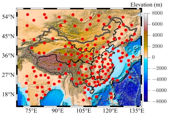
The study area is 15°N–55°N and 70°E–135°E, which covers the whole mainland China and its surrounding areas (see Figure 1). The terrain in China is overall higher in the southwest and lower in the east, with the altitude ranging from −154 m to 8848 m. In the study area, plains and basins occupy ~33% of the land area, and mountains, hills, and plateaus account for ~67%. Southwest China contains the Tibetan Plateau. Due to the complicated topography, the study area has diverse climate patterns, which are mainly dominated by dry seasons and wet monsoon. There are more than 100 radiosonde stations located in the study area, which provides sufficient data for experiments.
2.2. Data
2.2.1. Radiosonde Data
Radiosonde data are important meteorological observations, including pressure, temperature, relative humidity, etc., on certain pressure levels. In this study, we accessed radiosonde data from the Integrated Global Radiosonde Archive (IGRA). The IGRA provides high-quality sounding observations from more than 1500 radiosondes and sounding balloons worldwide since the 1960s and launches radiosonde twice daily at 00:00 and 12:00 UTC. All available meteorological profiles from 2007 to 2016 were collected and used to derive Tm according to the following equation [3]:
where h is the ellipsoidal height (km) in WGS84 (World Geodetic System 1984) frame converted from geopotential height, T denotes the temperature (K), e is the water vapor pressure (hPa), which is derived from relative humidity using the following equations:
where es denotes the saturated water vapor pressure (hPa), rh is the relative humidity, and Td is the atmospheric temperature (°C). The Tm time series at 00:00 and 12:00 UTC from 2007 to 2016 were computed at each radiosonde station. In total, 150 radiosonde stations were used at last, which are marked out in Figure 1.
2.2.2. GPT3 Model Predictions
The GPT3 model is the latest version of the GPT model [16]. The model provides empirical hydrostatic and wet delays, mapping functions, and other meteorological parameters. The meteorological parameters are directly taken from its predecessor, the GPT2w model, which provides temperature, pressure, water vapor pressure, and Tm. It uses a Fourier series to represent the temporal variations of the meteorological parameters, including Tm, on 5° × 5° or 1° × 1° grids. The temporal variations of the meteorological parameters are described as:
where r(t) indicates the meteorological parameters, doy means the day of year, A0 represents the mean value, A1 and B1 are the annual amplitudes, and A2 and B2 are the semi-annual amplitudes of the parameters.
3. Methods
The objective of this study is to improve the accuracy of empirical Tm using machine learning methods. The basic idea was to use the high-accuracy Tm derived from high-quality radiosonde observations to calibrate and optimize the Tm from empirical models through machine learning methods. To use the machine learning methods, the model structure should be set at first, which includes the selection of input and output and the determination of a specific machine learning structure. Furthermore, the model evaluation method should also be specified to assess the accuracy of different structures.
3.1. Selection of Input and Output
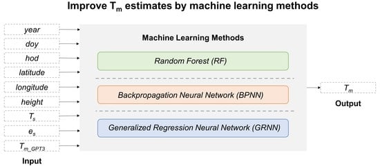
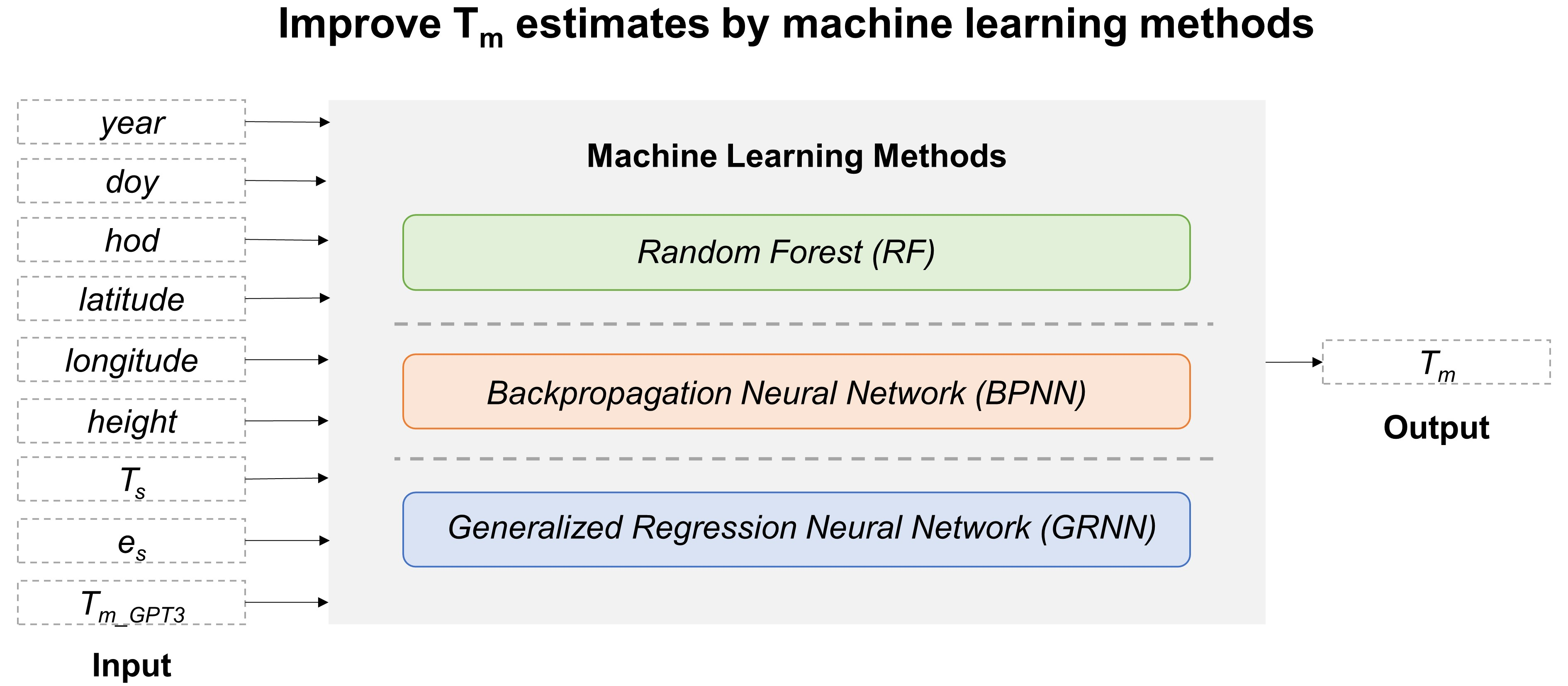
Since Tm has a strong correlation with surface temperature and water vapor pressure [4,22], the radiosonde measured temperature and water vapor pressure at the surface level were used as model input. In addition, empirical models have already well modeled the seasonal variations of Tm, which account for the majority of the temporal variations of Tm and can serve as good prior information for estimating more accurate Tm from machine learning models [18,19]. Therefore, the empirical Tm from the GPT3 model was also taken as one input to the machine learning models. When taking empirical Tm as an input, the high-quality radiosonde Tm is actually used to calibrate and optimize the empirical Tm through the machine learning models. To account for the spatial and temporal variations of Tm, the geographical information (latitude, longitude, height) and temporal information (year, day of year (doy), hour of day (hod)) were also taken as an auxiliary input to the machine learning model. The radiosonde is believed to be the most accurate approach to derive Tm by numerically integrating its vertical profiles of water vapor pressure and temperature [23,24]. The radiosonde-derived Tm were thus treated as target output of machine learning models. Consequently, the relationship between input variables and output Tm through machine learning methods can be written as:
where g() means machine learning-based estimation model, lat, lon, and h represent the three-dimensional geographical location, year, doy, and hod indicate the specific time, Ts is the surface temperature (K), es means the surface water vapor pressure (hPa), Tm_GPT3 denotes the Tm prediction from GPT3 model (K).
3.2. Machine Learning Structures
3.2.1. Random Forest (RF)
The RF technique is an ensemble learning method by constructing a multitude of decision trees at training time and outputting the mode of classes for classification or mean predictions for regression based on the bootstrap aggregation [25]. The decision tree algorithm in this study employs the classification and regression tree (CART), which can perform both the classification and regression tasks [26]. RF has the advantage of being able to account for complex and nonlinear relationships between input and output variables owing to its adaptive nature of decision rules.
The RF employs recursive partitioning to divide training data into many homogeneous subsets and builds multivariate regression trees with each subset based on a deterministic algorithm. For the growth of each regression tree, a bootstrap sample that contains about two-thirds of the samples is first selected from the training data. Then randomly selected input variables at each node are used to grow the tree by recursively partitioning the input space into successively smaller regions with binary splits. For the regression tree, the split point is determined by minimizing the regression error, which is a weighted sum of the regression error of each subset as shown in Equation (6):
where E(DL) and E(DR) are the regression errors of left and right subsets, N, NL, and NR are the number of total samples and the samples of left and right subsets, respectively. The regression algorithm computes the mean square error (MSE) as the regression error using Equation (7):
where y denotes the value of the target variable, denotes the average value of the target variable for all the samples. An individual regression tree is likely to overfit the data when it goes very deep, while RF can appropriately overcome this problem by introducing randomness into many individual regression trees and by averaging a large collection of these decorrelated individual trees to output the predictions with Equation (8):
where X indicates the input variables, Y is the final output of RF, Tb denotes the output of each individual regression tree, B is the number of trees.
3.2.2. Backpropagation Neural Network (BPNN)
The BPNN is one of the most commonly used artificial neural network (ANN) algorithms, which employs a gradient descent method to minimize the differences between the network output and target output [27]. It has the advantage of fitting a nonlinear relationship and thus, has been widely used in many regression problems.
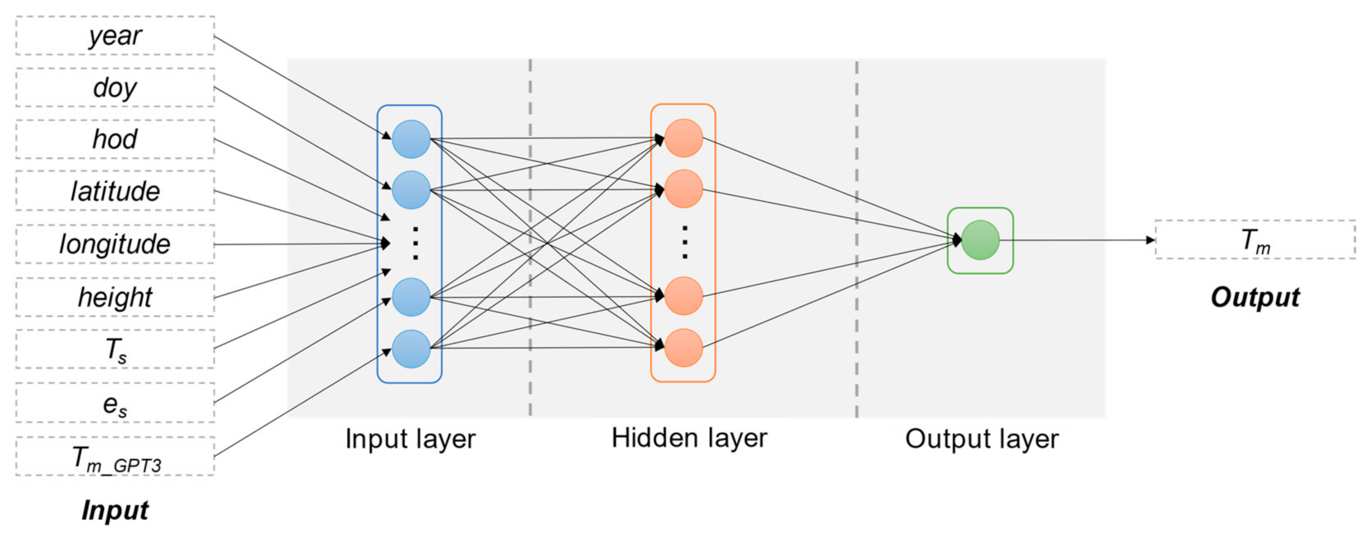
A BPNN model is composed of three different kinds of layers, i.e., an input layer, an output layer, and generally one hidden layer. The number of neurons in the input layer equals the number of input variables, and the number of neurons in the output layer equals the number of output variables. The determination of neuron number in the hidden layer is discussed later in Section 4.1. The structure of a BPNN model is shown in Figure 2.
In the BPNN model, each neuron in one layer is directly connected to the neurons of the subsequent layer with an activation function. In this study, we adopted the hyperbolic tangent function as the activation function of each neuron between the input and hidden layers, which is shown in Equation (9):
And we adopted the linear function as the activation function of each neuron between the hidden and output layers:
Then the final output of a BPNN can be written as:
where W2,1 and W3,2 are weight matrices and b1 and b2 are bias matrices, these four matrices store the coefficients of the BPNN model and should be optimized via the backpropagation algorithm [27], X and Y are the input and output variables.
3.2.3. Generalized Regression Neural Network (GRNN)
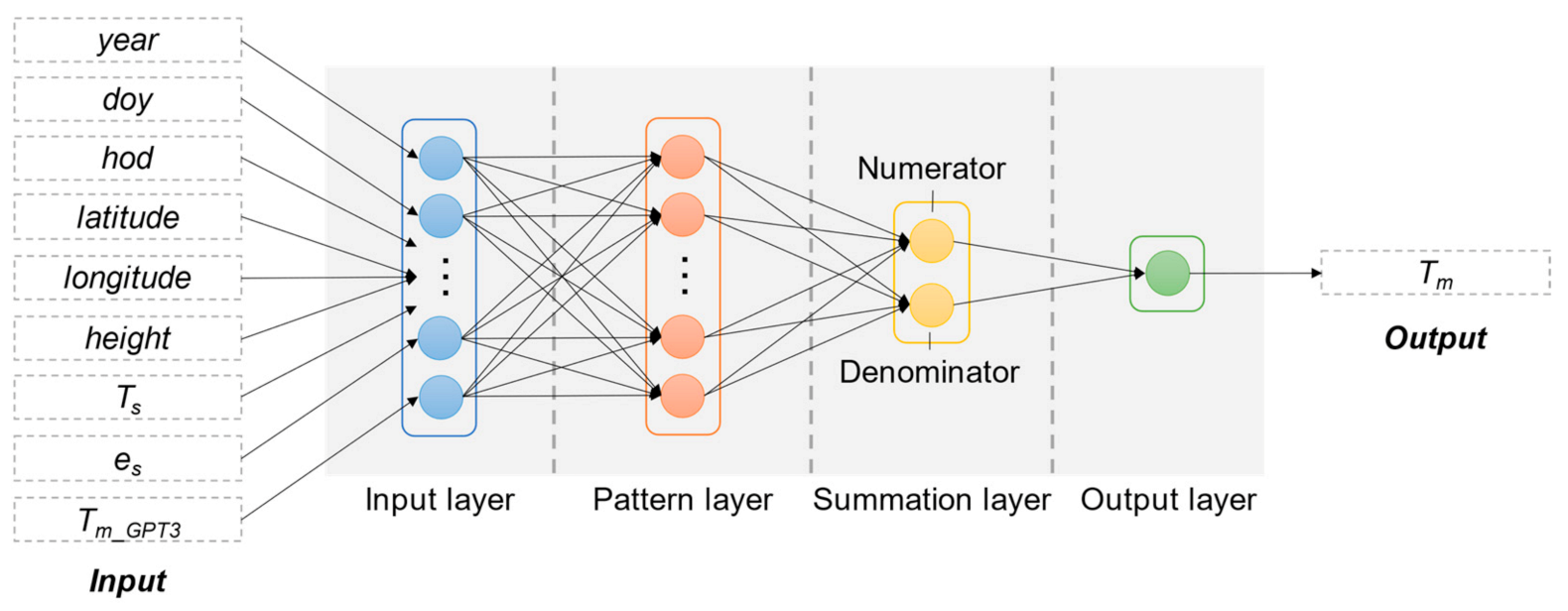
GRNN is a variation to the radial basis neural networks first suggested by [28]. It is a one-pass learning algorithm, which features fast learning without the requirement of an iterative procedure. GRNN is a powerful tool for regression, approximation, fitting, and prediction problems owing to its superiority in terms of fitting capability and convergence speed and can converge to the global minimum compared with BPNN.
The architecture of GRNN is composed of four layers: an input layer, a pattern layer, a summation layer, and an output layer. The number of neurons in the input layer equals the number of input variables. The number of neurons in the pattern layer equals the number of training samples. Each neuron in this layer is assigned with a sample vector Xi in the training data. If new input X is fed in, the Euclidean distance between the input vector X and the assigned vector Xi is first calculated using Equation (12):
where di denotes the Euclidean distance between X and Xi. The results are then fed into a Gaussian kernel as shown in Equation (13):
where K(·,·) stands for the Gaussian kernel, σ is called the “spread” parameter, which affects the level of fitness in GRNN architecture. Large values of the spread parameter tend to force the estimation to be smooth, while lower values provide a closer approximation to the sample values [28]. The spread is the only unknown parameter in the network and needs to be optimized. The determination of its optimum value is given in Section 4.1. The outputs of the pattern layer are sent to the summation layer. The summation layer is divided into two parts: a “Numerator” part and a “Denominator” part. The input to the Numerator neuron is the sum of the pattern layer outputs weighted by the sample output Yi corresponding to Xi in the training data. The input to the Denominator number is the sum of the pattern layer outputs. The output layer receives the two outputs from these two neurons in the summation layer and divides the Numerator output by the Denominator output, which is shown in Equation (14):
where n denotes the neuron number in the pattern layer, which equals the number of training samples. Therefore, GRNN memorizes every unique pattern in the training samples, which makes it a single-pass learning network without any backpropagation learning. The structure of the GRNN model is given in Figure 3.
3.3. Model Evaluation
The 10-fold cross-validation technique was used to evaluate the accuracy of different machine learning models [29]. This technique randomly and averagely divides the original dataset into 10 groups, where 9 groups are used as the training set for model fitting, and the remaining 1 group serves as the test set for model testing. This process should be repeated 10 times, and for each 10-fold cross-validation run, we computed and stored all the residuals. With this implementation, we could finally obtain the residual for each sample. We called these residuals the cross-validation residuals, hereafter. Based on the cross-validation residuals, we computed five statistical indicators, i.e., the Bias, mean absolute error (MAE), standard deviation (STD), root mean square error (RMSE), and Pearson correlation coefficient (R) to give a quantitative assessment of the model performances. The equations to compute these five indicators are given as:
where N indicates the number of samples, are the Tm values output from machine learning models, are the reference Tm values derived from radiosonde measurements, and are the mean values of and , respectively. In the 10-fold cross-validation technique, each sample was tested, and thus it can provide a reliable evaluation of the model accuracy. After performing the cross-validation, we used all the samples for model fitting to yield a final model for later prediction and gave the statistical indicators based on fitting residuals.
4. Results
4.1. Determining the Hyperparameter
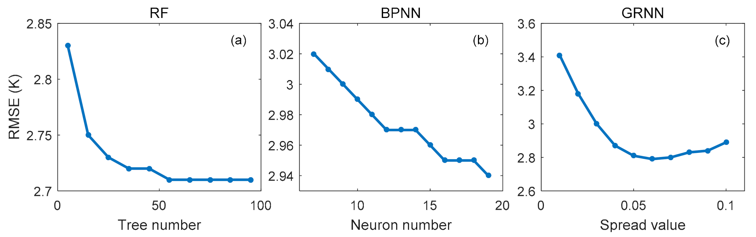
In this section, we determined the optimal hyperparameters for different machine learning methods, i.e., the number of trees for RF, the neuron number in the hidden layer for BPNN, and the spread value for GRNN. To determine the optimal number of trees in RF, we set the number from 5 to 95 with a step of 5 and then evaluated the performance of different RF models based on the 10-fold cross-validation technique. According to previous works [30,31], the optimum number of neurons in the hidden layer can be determined based on the range from to 2n + 1, where n and μ are the number of neurons in the input and output layer, respectively. In this study, n equaled 9 and μ equaled 1. We, therefore, tested a series of hidden layer neurons ranging from 7 to 19 for the BPNN model based on the 10-fold cross-validation technique. In the GRNN model, the adopted spread parameter usually ranges from 0.01 to 1 [32]. After many experiments, we found that the optimal spread value could be between 0 and 0.1. Therefore, we successively set the spread value of GRNN from 0.01 to 0.1 with a step of 0.01 for 10-fold cross-validation training for finalizing the best spread. Based on the cross-validation residuals, we computed the RMSE to compare the performances of different model settings. The RMSEs against the number of trees in RF, the neuron number in the hidden layer in BPNN, and the spread value in GRNN is depicted in Figure 4.
Figure 4a shows that for the RF model when the number of trees increased from 5 to 55, the RMSE decreased. However, the decrease stopped after the number of trees was greater than 55. Therefore, we set the number of trees as 55 for the RF model. Figure 4b shows that for the BPNN model, when the neuron number was in the range from 7 to 19, the RMSE decreased, and the RMSE was the smallest with the neuron number equal to 19. We also tested the case where the neuron number in the hidden layer was larger than 19. We found that when the neuron number was larger than 19, the RMSE still decreased, but the decrease rate was very small, and a very long training time was required. Hence, we set the neuron number in the hidden layer as 19 for the BPNN model. Figure 4c shows that for the GRNN model, the RMSE decreased when the spread value increased from 0.01 to 0.06 and is then followed by an increase when the spread value was larger than 0.06. Therefore, we finally determined the spread value as 0.06 for the GRNN model.
4.2. Overall Performance of the Model
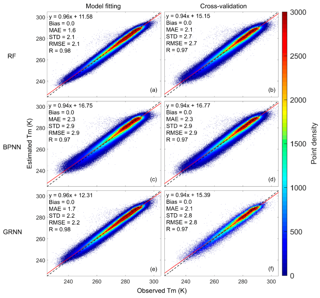
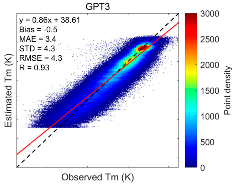
After determining the hyperparameters, we used all the training data (936,814 samples) to test the performances of different machine learning models using the 10-fold cross-validation technique. We computed the Tm from model fitting results and cross-validation results (estimated Tm) and showed their scatter plots against the radiosonde-derived Tm (observed Tm) in Figure 5. The empirical model GPT3 was also tested for comparison. The scatter plots of the Tm output from this model against the radiosonde-derived Tm are given in Figure 6. By removing the estimated Tm from observed Tm, we obtained the residuals, based on which we computed the Bias, MAE, STD, and RMSE. The correlation coefficient R between estimated Tm and observed Tm was also computed. All the statistical results are shown in Table 1.
Comparing Figure 5 and Figure 6, we find that the point distributions from the machine learning methods (Figure 5b,d,f) were much denser near the fitting line with a higher slope (0.94) and higher cross-validation R (0.97) than the point distribution of the GPT3 model (Figure 6) that showed a more dispersed scatter diagram with lower slope (0.86) and lower R (0.93).
Table 1 shows that the GPT3 model had a bias of −0.5 K, while the three machine learning methods had biases close to 0. This suggests that the GPT3 model still had some systematic bias, while the machine learning methods successfully calibrated these biases. As for the STD, which is free of systematic bias, the STDs from the three machine learning methods were apparently reduced compared with that from the GPT3 model. This is attributed to the machine learning methods optimizing the empirical Tm values from the GPT3 model via high-accuracy radiosonde-derived Tm values. The cross-validation RMSEs of the three machine learning models were largely reduced compared with that of the GPT3 model. The percentage RMSE reductions were 37.2%, 32.6%, and 34.9% for the RF model, the BPNN model, and the GRNN model compared with the GPT3 model. This indicates that the three machine learning methods significantly improved the accuracy of the GPT3 model. This is because we used high-accuracy radiosonde Tm to calibrate and optimize the GPT3 Tm via machine learning methods. Due to the strong capability of the machine learning methods in simulating complex nonlinear relations, the residuals between the radiosonde Tm and the GPT3 Tm were well modeled and corrected, consequently leading to higher accuracy of Tm estimates.
When comparing the three machine learning models, we found that the RF performs better than the BPNN and GRNN models by showing smaller cross-validation RMSE. Therefore, the RF model is believed to have the highest accuracy among the three machine learning models.
4.3. The Spatial Performance of the Models
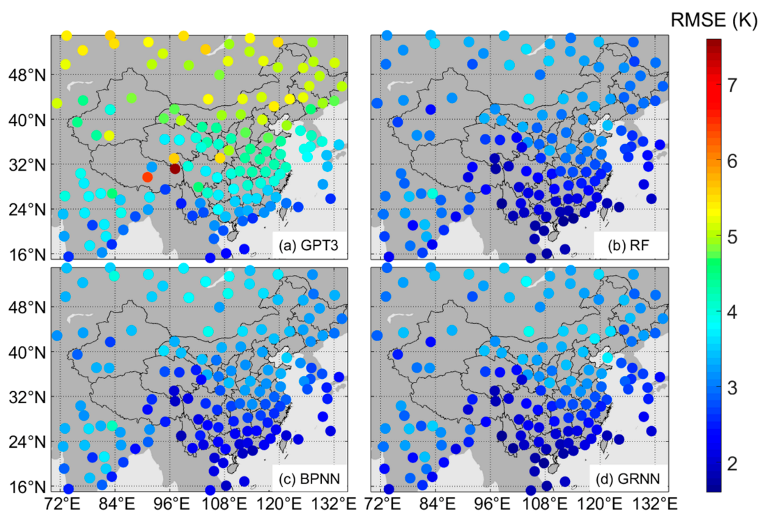
To give a comprehensive assessment of the performance of the machine learning models, we used their cross-validation residuals to compute the RMSE at each radiosonde station and show them in Figure 7. The RMSEs of the GPT3 model at each radiosonde station were also computed and shown in Figure 7 for comparison.
Figure 7 shows that the RMSEs were overall smaller in low latitude regions and larger in high latitude regions. This is because the seasonal variations of Tm are stronger in high latitude regions than in low latitude regions. Stronger seasonal variations bring more difficulties in Tm modeling, thus causing larger RMSE.
The RMSEs of the machine learning models were apparently smaller than that of the GPT3 model. The averaged RMSEs were 2.6 K, 2.9 K, and 2.7 K for the RF model, the BPNN model, and the GRNN model compared with 4.2 K for the GPT3 model. The number of sites with an RMSE value smaller than 3.0 K was 18 for the GPT3 model (Figure 7a), 90 for the RF model (Figure 7b), 72 for the BPNN model (Figure 7c), and 85 for the GRNN model (Figure 7d). These results demonstrate that the machine learning models have higher accuracy than the GPT3 model and that the RF model performs the best among these machine learning models.
In addition, Figure 7a shows that the RMSE of the GPT3 model was unevenly distributed in space, while the RMSEs of the machine learning models were much more evenly distributed, as shown in Figure 7b–d. This indicates that besides the accuracy improvement, the proposed machine learning methods also mitigate the accuracy variations in space compared with the GPT3 model, resulting in a more even spatial distribution of model accuracy. This is due to the geographical information, i.e., latitude, longitude, and height, which are input to the machine learning models. The GPT3 Tm are therefore calibrated and optimized differently in space.
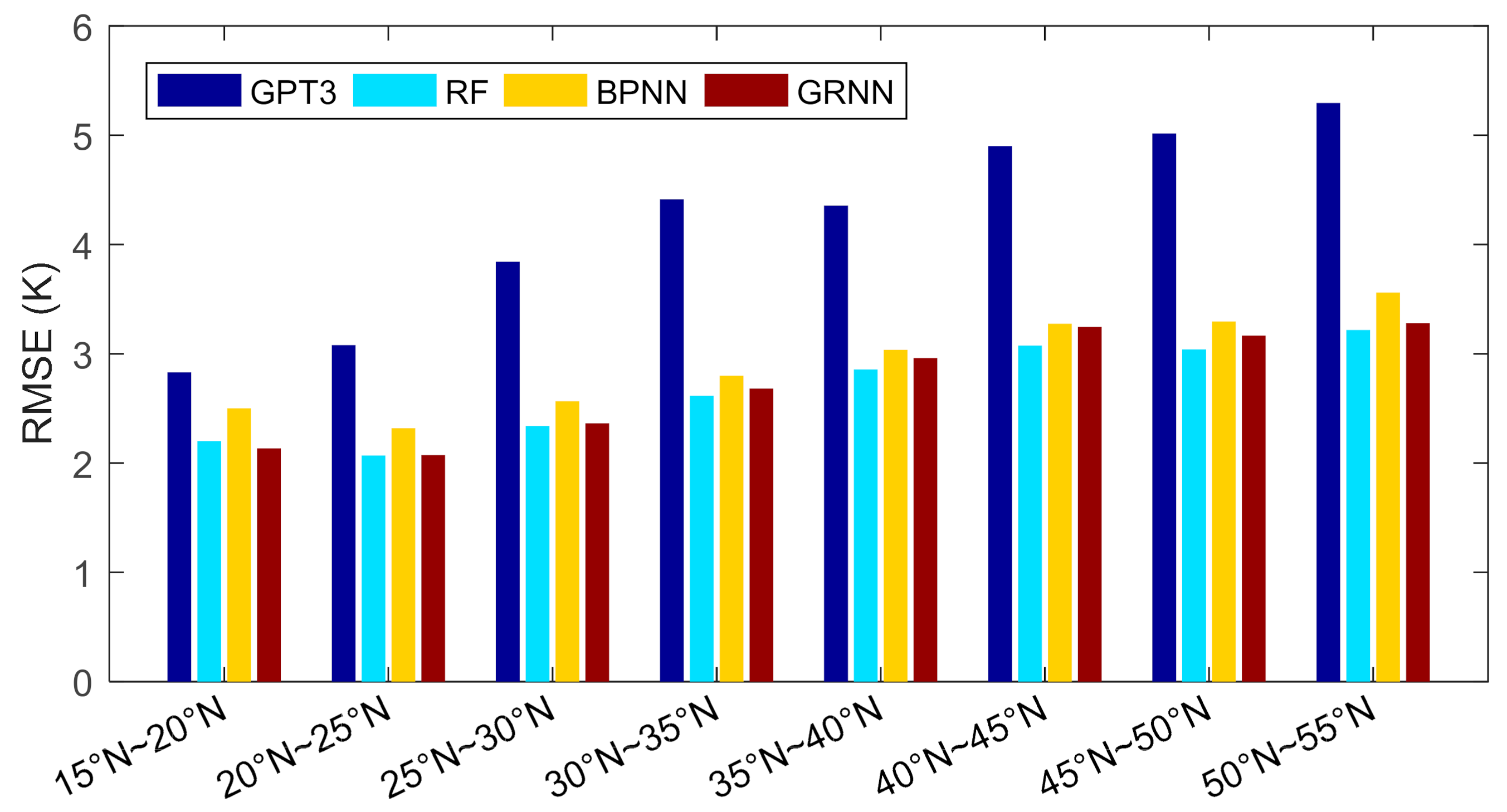
We further compared the performances of these models in different latitudes. We divided the research area into eight latitudinal bands with a sampling interval of 20°, and then computed the RMSEs of these models in each band based on the cross-validation residuals, which are shown in Figure 8 and Table 2.
Figure 8 shows that the RMSEs of these models overall increased with increasing latitudes, which is reasonable since the seasonal variations of Tm are stronger in higher latitudes than in lower latitudes. Stronger seasonal variations of Tm bring difficulties in modeling, which leads to larger RMSE in higher latitudes. In all the latitudinal bands, the RMSEs of the machine learning methods were smaller than those of the GPT3 model. Compared with the traditional empirical model GPT3, apparent RMSE reductions were achieved by machine learning methods. This indicates that the machine learning methods significantly improve the accuracy in estimating Tm than the GPT3 model. Comparing these three machine learning models, the RF model performs the best with slightly smaller RMSEs than the other two models, and the BPNN model is worse than the RF and the GRNN models by showing slightly larger RMSEs.
Furthermore, compared with the GPT3 model, the RMSE variations of the machine learning models with latitudes are more even. Table 2 shows that the RMSEs of the GPT3 model were smaller than 3 K at low latitudes and larger than 5 K at high latitudes. But the RMSEs of the machine learning models were within the range of 2 K and 3.5 K at these latitudes. This indicates that the machine learning methods effectively mitigate the accuracy variations in space, guaranteeing evenly high accuracy. This should be due to the geographical information being input into the machine learning models. The calibration and optimization of the GPT3 Tm are, therefore, different in space, which finally results in a more even spatial accuracy.
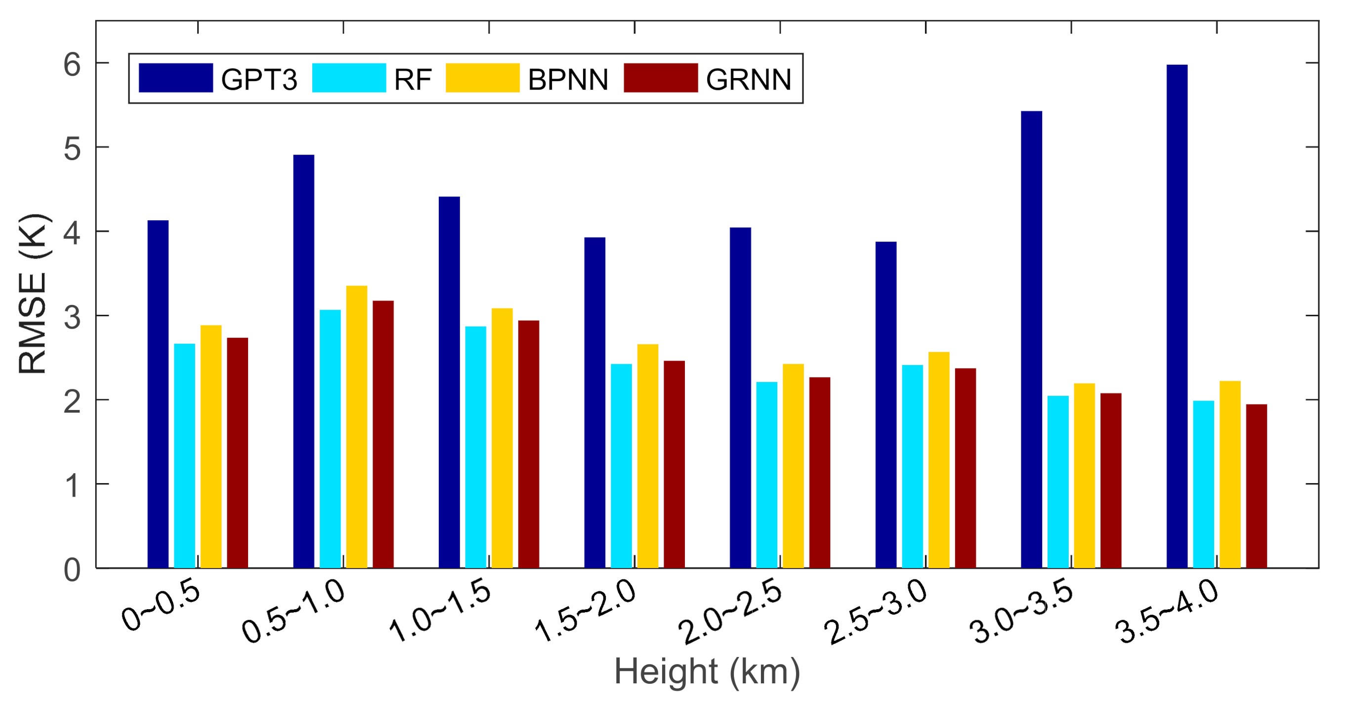
To evaluate the model performances in the vertical direction, we divided the height from 0 to 4 km into eight layers with a sampling interval of 0.5 km and calculated the RMSEs in each layer based on cross-validation residuals. The results are shown in Figure 9 and Table 3.
Figure 9 shows that the RMSE of the GPT3 model was overall smaller in lower heights and larger in higher heights. This should be due to the fact that the GPT3 model only estimates the Tm values near the surface and does not calibrate them in the vertical direction; thus, the RMSE of the GPT3 model is large in high heights. The RMSEs of the machine learning models overall decreased with increasing height. This is because, first, the machine learning models have calibrated the empirical Tm values from the GPT3 model in the vertical direction with height information input to the models, and second the magnitudes of Tm are smaller in higher heights. Smaller magnitudes lead to smaller RMSE. Therefore, the RMSEs of the machine learning models are smaller in higher heights.
The machine learning models had smaller RMSE than the GPT3 model in all the height layers, especially in higher heights where much larger RMSE reductions were observed. This indicates that the GPT3 model performs worse in estimating Tm at high heights, which is due to the fact that the GPT3 model does not perform height calibration to Tm estimates in the vertical direction, whereas the machine learning methods address this problem by calibrating the empirical Tm values with height and as a result, show small RMSE in high heights.
In addition, Figure 9 shows that the accuracy variation of the GPT3 model in the vertical direction was stronger than the machine learning models. According to Table 3, the RMSE of the GPT3 model was ~4 K at 0~0.5 km, increased to ~5 K at 0.5~1.0 km, and decreased to ~4 K at 1.5~3.0 km, and finally increased to 6 K at 3.5~4.0 km. However, the RMSEs of machine learning models were ~3 K at low heights and decreased to ~2 K at high heights. This indicates that the accuracy of the machine learning models is not only higher but also varies more evenly than the GPT3 model, which should be attributed to the fact that the height information is input to the machine learning models. As a result, the machine learning models, on the one hand, calibrate the empirical GPT3 Tm in the vertical direction; on the other hand, the calibration is different at different heights, which consequently generates a better and more even accuracy in the vertical direction.
4.4. The Temporal Performance of the Models
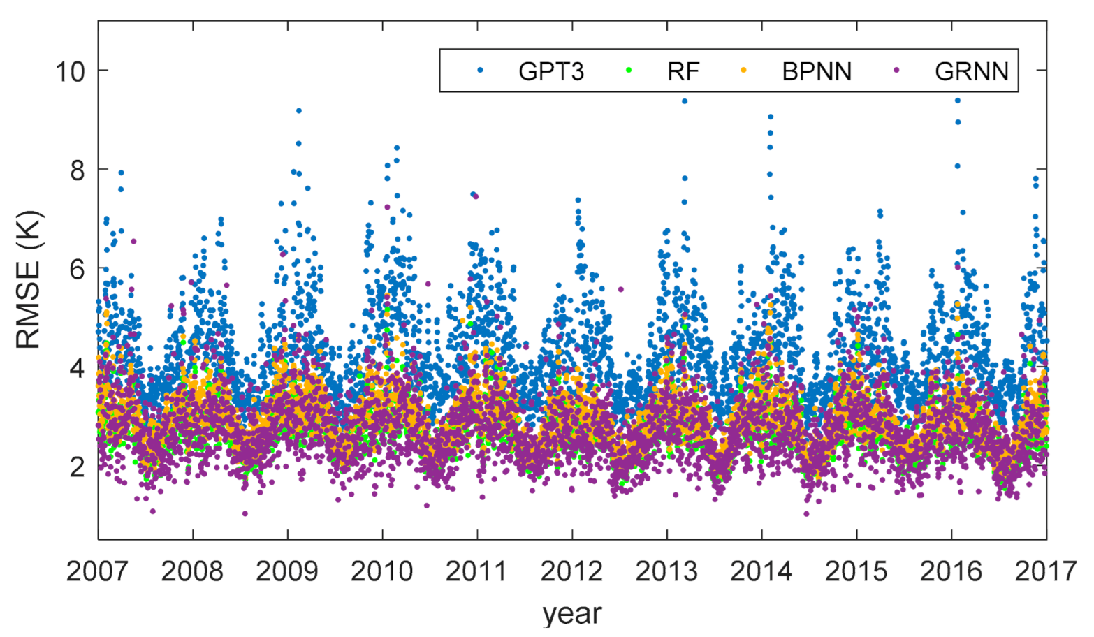
To investigate the temporal variation of the model performances, we used the cross-validation residuals to compute the RMSEs of different models for each day and display the results in Figure 10.
Figure 10 shows that the RMSEs were overall larger in winter and smaller in summer. This is because the seasonal magnitudes of Tm are larger in winter and smaller in summer. Larger seasonal magnitudes deteriorated the modeling results, leading to larger RMSE. Nearly in all the days, the RMSEs of the machine learning models were smaller than the GPT3 model, demonstrating the superiority of the machine learning methods. Moreover, the temporal variation of the accuracy of the GPT3 model was much stronger than the machine learning models. The RMSE of the GPT3 model was ~3 K in summer and reached 8 K in winter. Whereas for the machine learning models, the RMSEs were ~2 K in summer and ~4 K in winter. This indicates that compared with the GPT3 model, the proposed machine learning models effectively mitigate the accuracy variation in time, obtaining a more evenly temporal variation of accuracy. The reason for this is that the machine learning models consider the temporal difference in the accuracy of the Tm from the GPT3 model. The input variables of the machine learning models include time information; hence, the calibration and optimization of the GPT3 Tm via the machine learning models are different in time, which yields a more even temporal accuracy at last.
5. Discussion
5.1. The Reason for Accuracy Improvement of Machine Learning Models
To better understand the reason for the accuracy improvement of machine learning models, we plotted the estimated Tm time series from different models and compared them with radiosonde references. Figure 11 shows one exemplary plot at the radiosonde station CHM00057083 (34.71°N, 113.65°E).
Figure 11 shows that the GPT3 model could only simulate the seasonal pattern of Tm variations, while the machine learning models could simulate more complicated variations of Tm, such as the variations at synoptic scales. Therefore, the Tm time series estimated from the machine learning models agreed better with the radiosonde estimated ones than the GPT3 model. This could explain the accuracy improvement of Tm estimates from machine learning models.
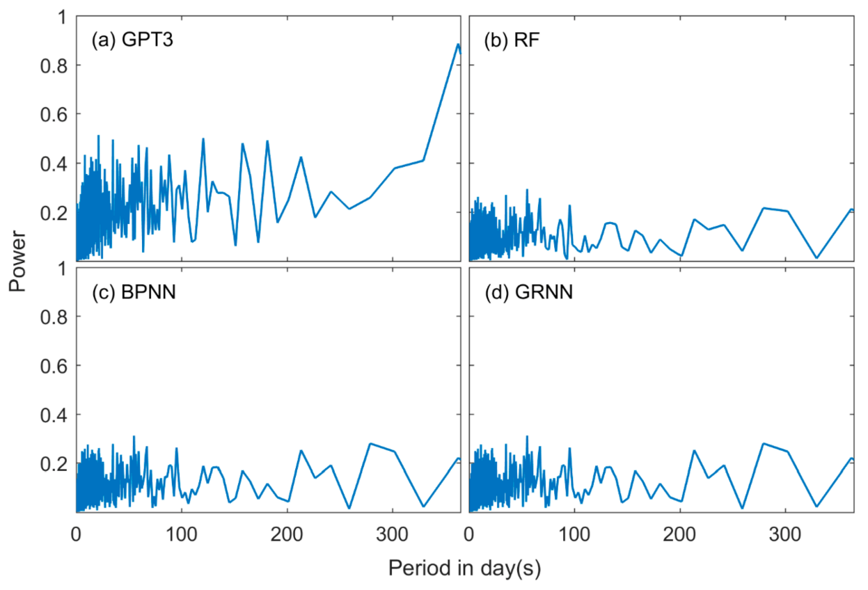
We further investigated the spectral characteristics of the residuals. We first computed the model residuals by removing the model output from the radiosonde-derived Tm and then applied Fast Fourier Transform (FFT) analysis to the residuals. We only focused on the spectral characteristics within one year since seasonal variations have been well modeled and interannual variation is not apparent in Tm. We used a high-pass filter to remove the low-frequency signals larger than one year before applying FFT. The exemplary power spectrums within one year at the station CHM00057083 (34.71°N, 113.65°E) are shown in Figure 12.
Figure 12a shows that the GPT3 model residuals had a strong power at high frequencies. The variations at these frequencies had timescales of several days to a few months, which were due to synoptic variations or irregular climate fluctuations that were not modeled by the GPT3 model. In addition, these variations changed with locations. These features make it hard to model these variations with a conventional method. These unmodeled variations bring uncertainties in Tm estimations and thus decrease the accuracy of the model. But Figure 12b–d shows that in the residuals of the machine learning models, the powers of these unclear frequencies were apparently mitigated, indicating that the machine learning methods can model these signals to some degree. This is because the machine learning methods are a data-adaptive approach, which can automatically learn the variation pattern of Tm from training data. Furthermore, the strong nonlinear fitting capacity of the machine learning methods can help well model the relationship between Tm and surface meteorological elements, which also benefits the modeling of the irregular variations. These results could explain the RMSE reductions in Tm of the machine learning models compared with the GPT3 model and further demonstrate that the proposed machine learning methods in this study could well simulate more complicated variations of Tm other than seasonal and diurnal variations.
5.2. Comparison of Computational Costs of Machine Learning Models
To better identify the advantages and disadvantages of different machine learning models, we compared their computational costs in terms of the time costs for model fitting and prediction and the memory space needed for storing the model. First, we recorded the time costs of model fitting and predictions for different machine learning models. Both the model fitting and prediction had 936,814 data samples to process. The implementations were conducted on MATLAB 2016 with a laptop computer equipped with Intel Core i7-8565U CPU at 1.80 GHz and the RAM of 8 Gigabytes (GB). The time costs of different models are given in Table 4. This table also gives the model size of different machine learning models.
Table 4 shows that the RF method took more than 3 min for model fitting, and the prediction took around 1 min. In the model fitting process, the RF method should continuously compute MSE on each node and grow the tree accordingly. Each tree finally grows around 120,000 nodes, and the whole forest (55 trees) have in total more than 6,500,000 nodes. The huge number of nodes requires large space memory to store the RF model, and its model size reaches approximately 6 GB. However, though the number of nodes is very large, the prediction of the RF model does not take much time. This is due to the fact that the implementations in the RF model are all judgments or decisions without any numerical calculations, which saves much time for predicting new values.
The BPNN model needed a long time for training (around 10 min), but the prediction of this model was very fast (around 5 s). This is because the BPNN method employs a backpropagation algorithm to continuously tune the weights and biases in the network, which requires an iterative procedure and takes a long time for training. But a well-trained BPNN model can output the prediction within a short time since this model uses very few coefficients (weights and biases) to compute the predictions. In this study, the BPNN model had only 210 coefficients in total. Due to the small number of coefficients, the memory space needed for storing the BPNN model was also very small, which was less than 25 Megabytes (MB) here.
The time cost of model fitting for the GRNN model was very small. This is because the GRNN method employs a one-pass learning algorithm without backpropagation training and iterative tuning. It simply memorizes all the samples and stores them in the network. Hence, the construction of a GRNN model is very fast, which only took 1 s here. But this model had much more coefficients than the BPNN model as it memorizes all the samples as the coefficients. Our GRNN model in this study had in total 10,304,954 coefficients, which, therefore, need more space for storage than the BPNN model and was around 40 MB here. The prediction of the GRNN model should compute the Euclidean distance between all the samples and the new input vectors, which requires a huge number of numerical calculations. The prediction by a GRNN model can be considered as an interpolation in multidimensional space, which thus takes a very long time and needs more than 10 h in this study.
6. Conclusions
In this study, we used machine learning methods to construct new Tm models in China based on random forest (RF), backpropagation neural network (BPNN), and generalized regression neural network (GRNN). Our new models could estimate Tm with the accuracies of 2.7 K, 2.9 K, and 2.8 K in terms of RMSE based on RF, BPNN, and GRNN, which significantly outperformed the traditional empirical model GPT3 with the RMSE reductions of 37.2%, 32.6%, and 34.9%, respectively. Moreover, the new models effectively mitigated the accuracy variations and achieved a more even accuracy in space and time. This is due to the fact that the new modeling methods based on machine learning have apparent superiority in modeling the irregular spatial and temporal variations of Tm.
However, this study only focuses on a national region, and the global data should be tested in the future. Moreover, this study only investigates the performance of machine learning methods, and the evaluation of deep learning methods is not included, which will be left for a future work.
Author Contributions
Conceptualization, Z.S. and B.Z.; Data curation, Z.S.; Formal analysis, Z.S. and B.Z.; Funding acquisition, B.Z. and Y.Y.; Investigation, Z.S. and B.Z.; Methodology, Z.S. and B.Z.; Project administration, B.Z. and Y.Y.; Resources, Z.S.; Software, Z.S.; Supervision, B.Z. and Y.Y.; Validation, Z.S.; Visualization, Z.S.; Writing—original draft, Z.S.; Writing—review & editing, B.Z. All authors have read and agreed to the published version of the manuscript.
Funding
This research was funded by the National Natural Science Foundation of China (NNSFC), grant number 42074035 and 41874033; the Fundamental Research Funds for the Central Universities, grant number 2042020kf0009; and the China Postdoctoral Science Foundation, grant number 2018M630880 and 2019T120687.
Institutional Review Board Statement
Not applicable.
Informed Consent Statement
Not applicable.
Data Availability Statement
The radiosonde data used in this paper can be freely accessed at https://www1.ncdc.noaa.gov/pub/data/igra/ (accessed on 1 March 2021). The GPT3 codes can be accessed at https://vmf.geo.tuwien.ac.at/codes/ (accessed on 1 March 2021). The training data and the machine learning codes related to this article can be found at https://github.com/sun1753814280/ML_Tm (accessed on 1 March 2021). The links for these data can be accessed all the time.
Acknowledgments
The authors would like to thank the Integrated Global Radiosonde Archive (IGRA) for providing the radiosonde data and Vienna University of Technology for providing the GPT3 codes.
Conflicts of Interest
The authors declare no conflict of interest.
References
- Leick, A. GPS satellite surveying. J. Geol. 1990, 22, 181–182. [Google Scholar]
- Askne, J.; Nordius, H. Estimation of Tropospheric Delay for Mircowaves from SurfaceWeather Data. Radio Sci. 1987, 22, 379–386. [Google Scholar] [CrossRef]
- Davis, J.L.; Herring, T.A.; Shapiro, I.I.; Rogers, A.E.E.; Elgered, G. Geodesy by radio interferometry: Effects of atmospheric modeling errors on estimates of baseline length. Radio Sci. 1985, 20, 1593–1607. [Google Scholar] [CrossRef]
- Bevis, M.; Businger, S.; Herring, T.A.; Rocken, C.; Anthes, R.A.; Ware, R.H. GPS meteorology: Remote sensing of atmospheric water vapor using the global positioning system. J. Geophys. Res. Atmos. 1992, 97, 15787–15801. [Google Scholar] [CrossRef]
- Bevis, M.; Businger, S.; Chiswell, S.; Herring, T.A.; Anthes, R.A.; Rocken, C.; Ware, R.H. GPS meteorology: Mapping zenith wet delays onto precipitable water. J. Appl. Meteorol. Clim. 1994, 33, 379–386. [Google Scholar] [CrossRef]
- Yao, Y.; Zhu, S.; Yue, S. A globally applicable, season-specific model for estimating the weighted mean temperature of the atmosphere. J. Geod. 2012, 86, 1125–1135. [Google Scholar] [CrossRef]
- Yao, Y.; Zhang, B.; Yue, S.; Xu, C.; Peng, W. Global empirical model for mapping zenith wet delays onto precipitable water. J. Geod. 2013, 87, 439–448. [Google Scholar] [CrossRef]
- Yao, Y.; Xu, C.; Zhang, B.; Cao, N. GTm-III: A new global empirical model for mapping zenith wet delays onto precipitable water vapour. Geophys. J. Int. 2014, 197, 202–212. [Google Scholar] [CrossRef] [Green Version]
- Chen, P.; Yao, W.; Zhu, X. Realization of global empirical model for mapping zenith wet delays onto precipitable water using NCEP re-analysis data. Geophys. J. Int. 2014, 198, 1748–1757. [Google Scholar] [CrossRef] [Green Version]
- He, C.; Wu, S.; Wang, X.; Hu, A.; Wang, Q.; Zhang, K. A new voxel-based model for the determination of atmospheric weighted mean temperature in GPS atmospheric sounding. Atmos. Meas. Tech. 2017, 10, 2045–2060. [Google Scholar] [CrossRef] [Green Version]
- Zhang, H.; Yuan, Y.; Li, W.; Ou, J.; Li, Y.; Zhang, B. GPS PPP derived precipitable water vapor retrieval based on Tm/Ps from multiple sources of meteorological data sets in China. J. Geophys. Res. Atmos. 2017, 122, 4165–4183. [Google Scholar] [CrossRef]
- Huang, L.; Jiang, W.; Liu, L.; Chen, H.; Ye, S. A new global grid model for the determination of atmospheric weighted mean temperature in GPS precipitable water vapor. J. Geod. 2019, 93, 159–176. [Google Scholar] [CrossRef]
- Yang, F.; Guo, J.; Meng, X.; Shi, J.; Zhang, D.; Zhao, Y. An improved weighted mean temperature (Tm) model based on GPT2w with T m lapse rate. GPS Solut. 2020, 24, 1–13. [Google Scholar] [CrossRef] [Green Version]
- Schüler, T. The TropGrid2 standard tropospheric correction model. GPS Solut. 2014, 18, 123–131. [Google Scholar] [CrossRef]
- Landskron, D.; Böhm, J. VMF3/GPT3: Refined discrete and empirical troposphere mapping functions. J. Geod. 2018, 92, 349–360. [Google Scholar] [CrossRef]
- Balidakis, K.; Nilsson, T.; Zus, F.; Glaser, S.; Heinkelmann, R.; Deng, Z.; Schuh, H. Estimating integrated water vapor trends from VLBI, GPS, and numerical weather models: Sensitivity to tropospheric parameterization. J. Geophys. Res. Atmos. 2018, 123, 6356–6372. [Google Scholar] [CrossRef] [Green Version]
- Sun, Z.; Zhang, B.; Yao, Y. A global model for estimating tropospheric delay and weighted mean temperature developed with atmospheric reanalysis data from 1979 to 2017. Remote Sens. 2019, 11, 1893. [Google Scholar] [CrossRef] [Green Version]
- Ding, M. A neural network model for predicting weighted mean temperature. J. Geod. 2018, 92, 1187–1198. [Google Scholar] [CrossRef]
- Ding, M. A second generation of the neural network model for predicting weighted mean temperature. GPS Solut. 2020, 24, 1–6. [Google Scholar] [CrossRef]
- Yang, L.; Chang, G.; Qian, N.; Gao, J. Improved atmospheric weighted mean temperature modeling using sparse kernel learning. GPS Solut. 2021, 25, 1–10. [Google Scholar] [CrossRef]
- Long, F.; Hu, W.; Dong, Y.; Wang, J. Neural Network-Based Models for Estimating Weighted Mean Temperature in China and Adjacent Areas. Atmosphere 2021, 12, 169. [Google Scholar] [CrossRef]
- Yao, Y.; Zhang, B.; Xu, C.; Yan, F. Improved one/multi-parameter models that consider seasonal and geographic variations for estimating weighted mean temperature in ground-based GPS meteorology. J. Geod. 2014, 88, 273–282. [Google Scholar] [CrossRef]
- Wang, J.; Zhang, L.; Dai, A. Global estimates of water-vapor-weighted mean temperature of the atmosphere for GPS applications. J. Geophys. Res. Atmos. 2005, 110. [Google Scholar] [CrossRef] [Green Version]
- Wang, X.; Zhang, K.; Wu, S.; Fan, S.; Cheng, Y. Water vapor weighted mean temperature and its impact on the determination of precipitable water vapor and its linear trend. J. Geophys. Res. Atmos. 2016, 121, 833–852. [Google Scholar] [CrossRef]
- Breiman, L. Random forests. Mach. Learn. 2001, 45, 5–32. [Google Scholar] [CrossRef] [Green Version]
- Breiman, L.; Friedman, J.; Stone, C.J.; Olshen, R.A. Classification and Regression Trees; CRC Press: Boca Raton, FL, USA, 1984. [Google Scholar]
- Hecht-Nielsen, R. Theory of the backpropagation neural network. In Neural Networks for Perception; Academic Press: Cambridge, MA, USA, 1992; pp. 65–93. [Google Scholar]
- Specht, D.F. A general regression neural network. IEEE Trans. Neural Netw. 1991, 2, 568–576. [Google Scholar] [CrossRef] [PubMed] [Green Version]
- Rodriguez, J.; Perez, A.; Lozano, J. Sensitivity analysis of k-fold cross-validation in prediction error estimation. IEEE Trans. Pattern Anal. Mach. Intell. 2009, 32, 569–575. [Google Scholar] [CrossRef] [PubMed]
- Gardner, M.; Dorling, S.R. Artificial neural networks (the multilayer perceptron)—A review of applications in the atmospheric sciences. Atmos. Environ. 1998, 32, 2627–2636. [Google Scholar] [CrossRef]
- Reich, S.; Gomez, D.; Dawidowski, L. Artificial neural network for the identification of unknown air pollution sources. Atmos. Environ. 1999, 33, 3045–3052. [Google Scholar] [CrossRef]
- Yuan, Q.; Xu, H.; Li, T.; Shen, H.; Zhang, L. Estimating surface soil moisture from satellite observations using a generalized regression neural network trained on sparse ground-based measurements in the continental US. J. Hydrol. 2020, 580, 124351. [Google Scholar] [CrossRef]
Figure 1.
Topography of the study area and geographical distribution of the radiosonde stations. The red points indicate the location of the radiosonde stations.
Figure 1.
Topography of the study area and geographical distribution of the radiosonde stations. The red points indicate the location of the radiosonde stations.

Figure 2.
Structure of backpropagation neural network (BPNN).

Figure 3.
Structure of generalized regression neural network (GRNN).

Figure 4.
Root mean square errors versus (a) the number of trees, (b) the neuron number in the hidden layer, and (c) the spread value derived from the 10-fold cross-validation technique.
Figure 4.
Root mean square errors versus (a) the number of trees, (b) the neuron number in the hidden layer, and (c) the spread value derived from the 10-fold cross-validation technique.

Figure 5.
Scatter plots of estimated the weighted mean temperature (Tm) against observed Tm for different models: (a) RF-model fitting; (b) RF-cross-validation; (c) BPNN-model fitting; (d) BPNN-cross-validation; (e) GRNN-model fitting; (f) GRNN-cross-validation. The dashed line is the 1:1 line. RF: random forest; BPNN: backpropagation neural network; GRNN: generalized regression neural network.

Figure 6.
Scatter plots of estimated Tm against observed Tm for GPT3 model. The dashed line is the 1:1 line. GPT3: global pressure and temperature model 3.
Figure 6.
Scatter plots of estimated Tm against observed Tm for GPT3 model. The dashed line is the 1:1 line. GPT3: global pressure and temperature model 3.

Figure 7.
Spatial distribution of the root mean square errors (RMSEs) at each radiosonde station for (a) GPT3 (global pressure and temperature model 3), (b) RF (random forest), (c) BPNN (backpropagation neural network), and (d) GRNN (generalized regression neural network).
Figure 7.
Spatial distribution of the root mean square errors (RMSEs) at each radiosonde station for (a) GPT3 (global pressure and temperature model 3), (b) RF (random forest), (c) BPNN (backpropagation neural network), and (d) GRNN (generalized regression neural network).

Figure 8.
Root mean square errors of different models at different latitude bands.

Figure 9.
Root mean square errors of different models at different height layers.

Figure 10.
Root mean square errors of different models at different days.

Figure 11.
Tm time series estimated from different models and radiosonde observations at the station CHM00057083 (34.71°N, 113.65°E).
Figure 11.
Tm time series estimated from different models and radiosonde observations at the station CHM00057083 (34.71°N, 113.65°E).

Figure 12.
Power spectrums of Tm residuals from (a) GPT3 (global pressure and temperature model 3), (b) RF (random forest), (c) BPNN (backpropagation neural network), and (d) GRNN (generalized regression neural network) models at the station CHM00057083 (34.71°N, 113.65°E).
Figure 12.
Power spectrums of Tm residuals from (a) GPT3 (global pressure and temperature model 3), (b) RF (random forest), (c) BPNN (backpropagation neural network), and (d) GRNN (generalized regression neural network) models at the station CHM00057083 (34.71°N, 113.65°E).


Table 1.
Model fitting and cross-validation performances of different models.
| Model | Model Fitting | Cross-Validation | ||||||||
|---|---|---|---|---|---|---|---|---|---|---|
| Bias | MAE | STD | RMSE | R | Bias | MAE | STD | RMSE | R | |
| GPT3 | −0.5 | 3.4 | 4.3 | 4.3 | 0.93 | |||||
| RF | 0.0 | 1.6 | 2.1 | 2.1 | 0.98 | 0.0 | 2.1 | 2.7 | 2.7 | 0.97 |
| BPNN | 0.0 | 2.3 | 2.9 | 2.9 | 0.97 | 0.0 | 2.3 | 2.9 | 2.9 | 0.97 |
| GRNN | 0.0 | 1.7 | 2.2 | 2.2 | 0.98 | 0.0 | 2.1 | 2.8 | 2.8 | 0.97 |
MAE: mean absolute error; STD: standard deviation; RMSE: root mean square error; R: Pearson correlation coefficient; GPT3: global pressure and temperature model 3; RF: random forest; BPNN: backpropagation neural network; GRNN: generalized regression neural network.
Table 2.
Root mean square errors of different models at different latitude bands.
| Latitude Band | RMSE (K) | |||
|---|---|---|---|---|
| GPT3 | RF | BPNN | GRNN | |
| 15°N~20°N | 2.8 | 2.2 | 2.5 | 2.1 |
| 20°N~25°N | 3.1 | 2.1 | 2.3 | 2.1 |
| 25°N~30°N | 3.8 | 2.3 | 2.6 | 2.4 |
| 30°N~35°N | 4.4 | 2.6 | 2.8 | 2.7 |
| 35°N~40°N | 4.4 | 2.9 | 3.0 | 3.0 |
| 40°N~45°N | 4.9 | 3.1 | 3.3 | 3.2 |
| 45°N~50°N | 5.0 | 3.0 | 3.3 | 3.2 |
| 50°N~55°N | 5.3 | 3.2 | 3.6 | 3.3 |
Table 3.
Root mean square errors of different models at different height layers.
| Height Layer | RMSE (K) | |||
|---|---|---|---|---|
| GPT3 | RF | BPNN | GRNN | |
| 0 km~0.5 km | 4.1 | 2.7 | 2.9 | 2.7 |
| 0.5 km~1.0 km | 4.9 | 3.1 | 3.4 | 3.2 |
| 1.0 km~1.5 km | 4.4 | 2.9 | 3.1 | 2.9 |
| 1.5 km~2.0 km | 3.9 | 2.4 | 2.7 | 2.5 |
| 2.0 km ~2.5 km | 4.0 | 2.2 | 2.4 | 2.3 |
| 2.5 km~3.0 km | 3.9 | 2.4 | 2.6 | 2.4 |
| 3.0 km~3.5 km | 5.4 | 2.0 | 2.2 | 2.1 |
| 3.5 km~4.0 km | 6.0 | 2.0 | 2.2 | 1.9 |
Table 4.
Time costs for model fitting and prediction and model size of different machine learning models.
Table 4.
Time costs for model fitting and prediction and model size of different machine learning models.
| Machine Learning Model | Time Cost | Model Size | |
|---|---|---|---|
| Model Fitting | Prediction | ||
| RF | 3′13′′ | 0′52′′ | 5889.6 MB |
| BPNN | 8′54′′ | 0′05′′ | 23.6 MB |
| GRNN | 0′01′′ | 11h33′54′′ | 39.2 MB |
Publisher’s Note: MDPI stays neutral with regard to jurisdictional claims in published maps and institutional affiliations. |
© 2021 by the authors. Licensee MDPI, Basel, Switzerland. This article is an open access article distributed under the terms and conditions of the Creative Commons Attribution (CC BY) license (http://creativecommons.org/licenses/by/4.0/).
Share and Cite
MDPI and ACS Style
Sun, Z.; Zhang, B.; Yao, Y. Improving the Estimation of Weighted Mean Temperature in China Using Machine Learning Methods. Remote Sens. 2021, 13, 1016. https://0-doi-org.brum.beds.ac.uk/10.3390/rs13051016
AMA Style
Sun Z, Zhang B, Yao Y. Improving the Estimation of Weighted Mean Temperature in China Using Machine Learning Methods. Remote Sensing. 2021; 13(5):1016. https://0-doi-org.brum.beds.ac.uk/10.3390/rs13051016
Chicago/Turabian StyleSun, Zhangyu, Bao Zhang, and Yibin Yao. 2021. "Improving the Estimation of Weighted Mean Temperature in China Using Machine Learning Methods" Remote Sensing 13, no. 5: 1016. https://0-doi-org.brum.beds.ac.uk/10.3390/rs13051016
Note that from the first issue of 2016, this journal uses article numbers instead of page numbers. See further details here.