
Accuracy Analysis of GNSS Hourly Ultra-Rapid Orbit and Clock Products from SHAO AC of iGMAS


Shanghai Astronomical Observatory, Chinese Academy of Sciences, 80 Nandan Road, Shanghai 200030, China
*
Author to whom correspondence should be addressed.
Remote Sens. 2021, 13(5), 1022; https://0-doi-org.brum.beds.ac.uk/10.3390/rs13051022
Submission received: 31 December 2020
/
Revised: 28 February 2021
/
Accepted: 3 March 2021
/
Published: 8 March 2021
(This article belongs to the Special Issue Upcoming Positioning, Navigation and Timing: GPS, GLONASS, Galileo and BeiDou)
Abstract
:With the development of the global navigation satellite system(GNSS), the hourly ultra-rapid products of GNSS are attracting more attention due to their low latency and high accuracy. A new strategy and method was applied by the Shanghai Astronomical Observatory (SHAO) Analysis Center (AC) of the international GNSS Monitoring and Assessment Service (iGMAS) for generating 6-hourly and 1-hourly GNSS products, which mainly include the American Global Positioning System (GPS), the Russian Global’naya Navigatsionnaya Sputnikova Sistema (GLONASS), the European Union’s Galileo, and the Chinese BeiDou navigation satellite system (BDS). The 6-hourly and 1-hourly GNSS orbit and clock ultra-rapid products included a 24-h observation session which is determined by 24-h observation data from global tracking stations, and a 24-h prediction session which is predicted from the observation session. The accuracy of the 1-hourly orbit product improved about 1%, 31%, 13%, 11%, 23%, and 9% for the observation session and 18%, 43%, 45%, 34%, 53%, and 15% for the prediction session of GPS, GLONASS, Galileo, BDS Medium Earth Orbit (MEO), Inclined Geosynchronous Orbit (IGSO), and GEO orbit, when compared with reference products with high accuracy from the International GNSS service (IGS).The precision of the 1-hourly clock products can also be seen better than the 6-hourly clock products. The accuracy and precision of the 6-hourly and 1-hourly orbit and clock verify the availability and reliability of the hourly ultra-rapid products, which can be used for real-time or near-real-time applications, and show encouraging prospects.
1. Introduction
The Global Navigation Satellite System (GNSS) has achieved remarkable progress in modernization and global service capacity in recent decades. The American Global Positioning System (GPS) and Russian Global’naya Navigatsionnaya Sputnikova Sistema (GLONASS) are enabling full global coverage services and are undergoing modernization. Moreover, the new global navigation satellite systems, such as the Galileo satellite navigation system(Galileo) established by the European Union (EU), and the Chinese BeiDou navigation satellite system (BDS) were launched to improve global and regional coverage, in order to provide more improved services to users [1,2,3,4]. Some countries have also claimed regional navigation satellite projects, such as Japan, India, and South Korea [5,6].
The multi-frequency signals are transmitted from the GNSS constellations, which can be received and used by global users conveniently. Moreover, there are great challenges and opportunities for satellite positioning, timing, and navigation (PNT) for more and more satellites, observation frequencies and types which can benefit users for many applications [7,8,9].
Some organizations have studied GNSS in past decades. International GNSS Services (IGS) was founded in 1996 and provides GNSS observation data and products to support the terrestrial reference frame, PNT, and other scientific research and engineering applications [10].
The network of IGS stations has grown rapidly in recent years, reaching more than 500 stations distributed all over the world, about two-thirds of which have been updated to track GNSS, and could upload daily, hourly, and high-rate observation data files to the IGS Data Center (DC) [10]. The IGS Analysis Center (AC), which retrieves the observation data from DCs, can generate products to IGS, for combination, and then provide to the users. The IGS provides official final, rapid, and ultra-rapid products of GPS and GLONASS to users (www.igs.org). However, the combined orbit and clock products of new constellations, such as BDS and Galileo, are still missing in the IGS official products.
IGS launched the Multi-GNSS Experiment (MGEX) project in 2011, and then started a pilot project in 2016 after the experimental phase ended. The MGEX station network was established or updated from the IGS reference network, which could receive radio signals transmitted from BDS, Galileo, and the Japanese Quasi-Zenith Satellite System (QZSS), as well as legacy GPS and GLONASS. More MGEX observation data files were named (by longname) with RINEX version 3, which can be downloaded from IGS/MGEX DCs. Many ACs, such as the Center for Orbit Determination in Europe (CODE), GeoForschungsZentrum (GFZ), Shanghai Astronomical Observatory (SHAO), and Wuhan University etc., can provide GNSS orbit and clock products for MGEX. However, the combined MGEX products have not been available until now by MGEX [2].
The international GNSS Monitoring and Assessment System (iGMAS), which was initiated by China, is an open technology platform for the collection, storing, analysis, and managing observation data, and can provide relative products and evaluation performance of GNSS [1,7]. iGMAS consists of 30 global tracking stations, three DCs, and more than seven ACs. The ACs of iGMAS can provide GNSS products with high precision, including orbits, clock, station coordinates, earth rotation parameters (ERP), zenith troposphere delay (ZTD), and global ionosphere delay. These products include three types: final, rapid, and ultra-rapid (www.igmas.org). The ultra-rapid orbit and clock products of IGS or iGMAS comprise of observation and prediction sessions. The predicted session, especially the predicted orbit, can be used to estimate real-time clock offset for real-time precise point positioning (PPP). The predicted clock can also be used as an initial value to estimate the real-time clock. However, the lack or latency of observation data in the predicted session decreases the accuracy of the predicted orbit and clock [11]. Moreover, the latency of ultra-rapid products is usually 3 h, meaning that the user can only exploit the predicted orbit and clock from the first to the ninth hour in the prediction session.
With notable developments of PPP theory, the real-time PPP has attracted more interest and will be widely applied in navigation, automatic piloting, atmospheric sounding, natural disasters, hazard monitoring, and rescue, etc. [12]. However, the time consumption, timeliness, and accuracy of the ultra-rapid orbit and clock products are the main issues for real-time studies or applications. More global distribution stations and constellations should be processed to generate the products if we want to pursue better accuracy and precision. However, it will cause more time consumption and increase latency so as to hardly satisfy the real-time or near-real-time users. Thus, the methods for increasing the updated rate of ultra-rapid orbit and clock products have been studied by many researchers.
Choi et al. (2012) have studied the accuracy of ultra-rapid products from the ACs of IGS and combined IGU products, assessed by rapid products. They found that the 40–45 h observation arc length can generate better predicted orbit than a 1 day case [13]. Li et al. (2019) studied the improved method to produce hourly ultra-rapid products with about 100 stations, which cost about 50 min [8]. A method was studied by Ma, which was used to generate hourly ultra-rapid orbit products by combining normal equations from two solutions: a 22-h solution plus a 3-h solution. This method improved the latency of the products. Nevertheless, there is a problem in this method for hardly fixing the ambiguities if the cycles exist between the joints of the two solutions [11].
However, the stability, continuity, latency, and accuracy should be improved for previous studies. More observation data from stations should be available, and the computation efficiency and optimized method should be studied to shorten the latency and update interval in order to achieve the predicted orbit and clock products, with high accuracy and low latency. This article presents a new strategy and method to generate the hourly ultra-rapid orbit and clock products, which may be different from previous studies. Then, the accuracy of the products are analyzed.
2. Data, Methods, and Strategy
In recent years, more IGS/MGEX stations were updated to track Galileo and BDS, as well as QZSS and Indian Regional Navigation Satellite System (IRNSS) satellites. The data observed from stations were archived in the DCs from IGS/MGEX, which can be downloaded freely. However, the distribution of the stations, which can track the BDS and Galileo, are not as good as GPS and GLONASS. Thus, in this contribution, the observation data from stations of iGMAS, which are distributed globally, and the Crustal Movement Observation Network of China (CMONOC), mainly distributed in the Chinese mainland, are used.
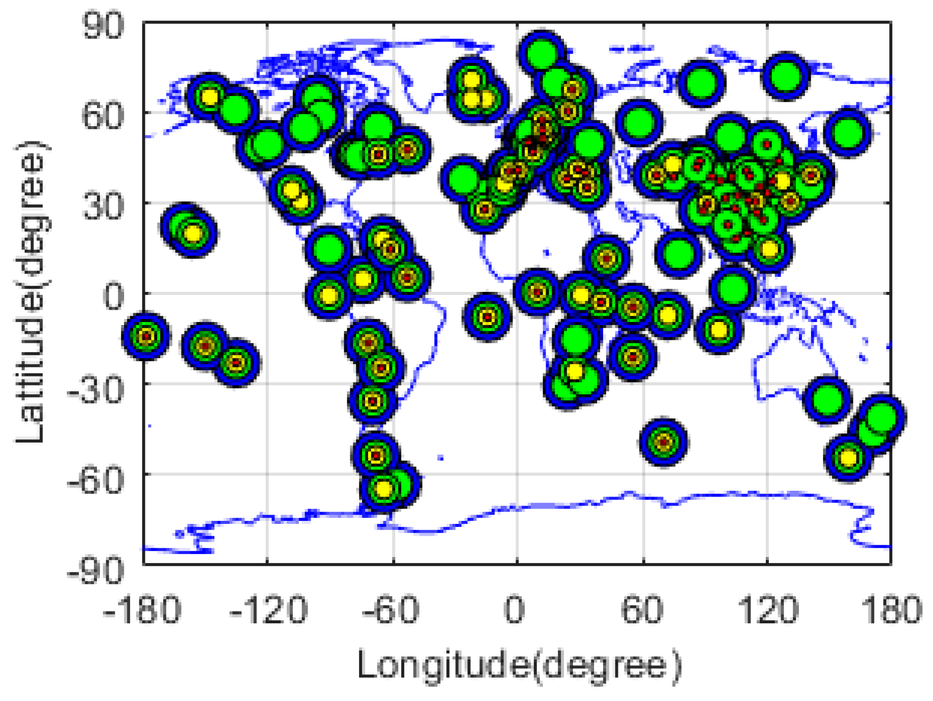
Approximately 120 stations are used to generate the hourly ultra-rapid orbit and clock products in this study, which include 60–70 stations that can receive BDS and Galileo observation data, as shown in Figure 1. The blue circles represent the stations, which can track GPS satellites; the green circles represent stations tracking GLONASS; the yellow circles show the stations tracking Galileo, and the red circles represent the stations tracking BDS satellites.
In order to improve the efficiency for downloading the observation data and broadcast ephemeris, the optimized parallel scripts are coded with a remote scanning method in the Linux server, which runs by an automatic operation mode to retrieve data from IGS/MGEX DCs, such as the Crustal Dynamics Data Information System (CDDIS), Instituto Geográfico Nacional (IGN), The Federal Agency for Cartography and Geodesy (BKG) and Chinese tracking station networks from iGMAS and CMONOC.
A new method—combined serial and parallel threads (CSPT)—is studied in this contribution. It is different from previous studies [8,11] when it comes to improving the stability and reliability of the products—avoiding some problems that may be caused by satellites (from a single satellite system), and reducing the time consumption and latency of the ultra-rapid orbit and clock products. The CSPT method is introduced in the Appendix A.
Table 1 shows the strategy of the CSPT method for GNSS product generation in this study. This method includes four serial threads, which were operated in parallel mode, and arranged to generate the hourly orbit and clock products for GPS, GLONASS, Galileo, and BDS. Moreover, the GLONASS, Galileo, and BDS were coupled with GPS in their threads to improve the accuracy of their products. The inter-system biases (ISBs) were estimated in the coupled satellite systems for Galileo and BDS, while the inter-frequency bias (IFB) parameters were estimated as constants, without constrains, for each GLONASS satellite and station pair, for the Frequency Division Multiple Access (FDMA), applied by GLONASS to recognize the different satellites.
Full operational capability (FOC) satellites should be included in the products as much as possible, in order to provide better service to users. In this study, about 32 and 24 Medium Earth Orbit (MEO) satellites were included for GPS and GLONASS, which were established earlier and showed a notable performance. Moreover, about 24 MEO satellites for Galileo, and five Geostationary Orbits (GEO), five satellites in Inclined Geosynchronous Orbit (IGSO), and four MEO for BDS-2 satellites were also included in this contribution.
The undifferenced (UD) ionosphere-free (IF) combinations for double frequency observations, such as L1 (1575.42 MHz) and L2 (1227.60 MHz) frequencies for GPS, GLONASS L1 (1602.00 MHz) and L2 (1246.00 MHz), Galileo E1 (1575.42 MHz) and E5a (1176.45 MHz), BDS-2 B1 (1561.098 MHz) and B2 (1207.14 MHz), were formed to eliminate the first order of ionospheric delays. The cutoff elevation angle of the observation data was selected at 7 degrees. The sampling intervals were 450 and 600 s for 6-hourly (6H) products and 1-hourly (1H) products, respectively, in order to improve the data processing efficiency.
Then, the orbit and clock parameters were estimated from the carrier phase and pseudorange observations. The clock of satellites and receivers were estimated at every sampling interval. Moreover, a reference clock from a station was fixed as the time reference, which was usually connected with a hydrogen atomic clock and showed better performance.
The force models, such as the solar radiation pressure (SRP) with five parameters, Earth gravity model (EGM) with degree and order 12, solid earth tide, pole tide, M-body gravity model (DE405), and phase win-up corrections [15] were applied for orbit estimation. The ocean tide loading corrections of each station were retrieved from the Onsala Space Observatory (OSO), which is the component of the Swedish National Infrastructure [16].
The ambiguity solutions needed to be determined in order to improve the accuracy of the parameters estimation [17]. However, the float ambiguity solutions were calculated for GLONASS and BDS GEO, which were hard to fix because of the distinctive signal transmit mechanism for GLONASS and special satellite slot for BDS GEO.
The phase center correct (PCC) must be considered for improving the accuracy of the products. PCC files of the antenna of the stations and GPS/GLONASS/Galileo satellites can be downloaded from IGS [18,19], while PCC of BDS are referred to reference [14].
Saastamoinen established the ZTD model, which was called the Saastamoinen model by many researchers [20]. Chen et al. (2011) assessed the Saastamoinen model and found the accuracy of the model was about 4 cm [21]. Boehm studied and established the global mapping function (GMF), which was used by many researchers and engineers [22,23,24,25]. The Saastamoinen model and GMF were used to estimate ZTD in this contribution. The interval of ZTD was estimated by piecewise constant (PWC), with a 1-h interval, while the interval of horizontal gradient was 12 h.
The initial parameters of ERP were achieved from International Earth Rotation and Reference Systems Service (IERS) rapid products, which were strongly constrained during the parameters estimation. Moreover, the ERP parameters were also updated during the running CSPT.
The reference frame of the orbit and clock products was based from the ITRF2014. The initial coordinates and constrain information of the stations from IGS/MGEX were downloaded from IGS weekly final solution independent exchange (SINEX) format solutions. However, the initial coordinates of stations from iGMAS or CMONOC could be extracted from the final solution of SHAO AC of iGMAS with loose constrains.
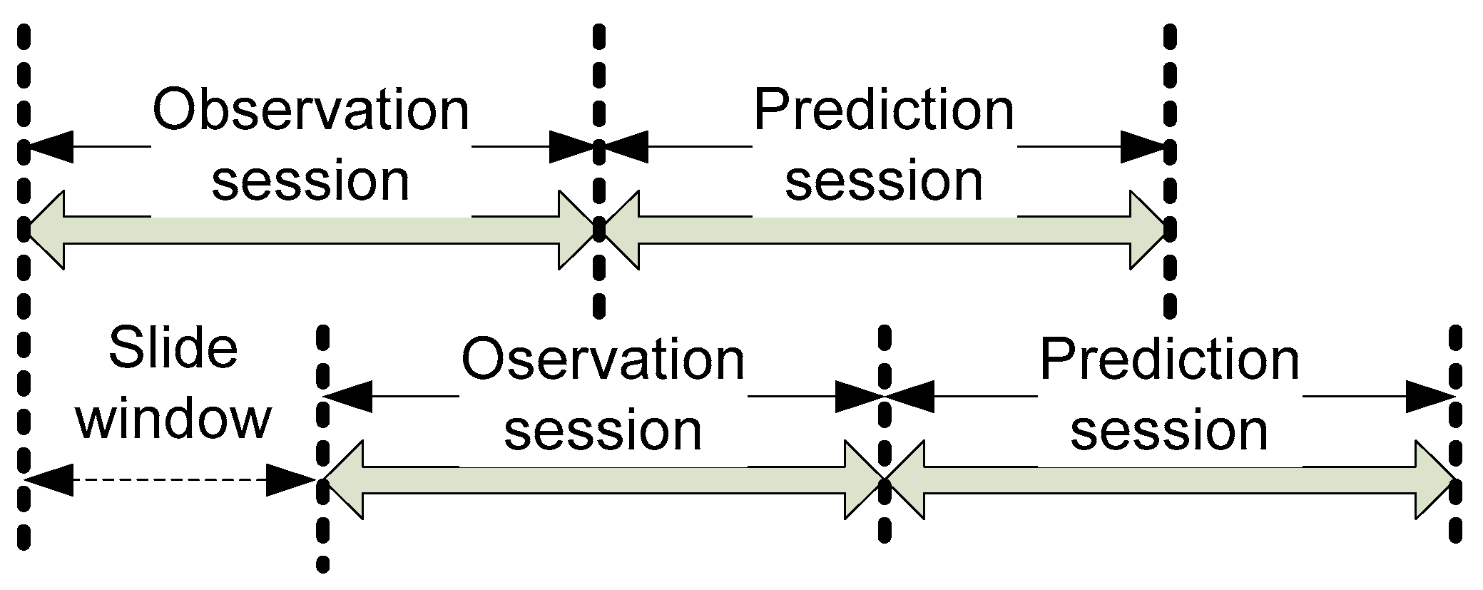
Figure 2 shows the slide window for hourly ultra-rapid orbit and clock products. The slide window was 6 h for 6-hourly GNSS orbit and clock productions, which were similar to IGS ultra-rapid products, while a 1-h slide window was applied for 1-hourly productions. Moreover, Figure 2 shows the ultra-rapid productions were comprised of a 24-h observation session and a 24-h prediction session.
Some studies found that a long arc-length, such as a 25–40 h length, could get a better prediction orbit [8,11,13]. However, time consumption is an issue for the latency of the products. Thus, in this study, we discussed a new prediction strategy which fit two-day orbits to integrate the orbit for the prediction orbit, while the prediction clock was computed by a modified Auto Regressive Integrated Moving Average (ARIMA) method [26].
The daily-observed data are not suited to generate the ultra-rapid orbit and clock productions for their long latency, and the fixed whole day observation session. Thus, the hourly observation data are extremely important, and combined for each station, according to the given session set by users to generate the hourly ultra-rapid productions.
The raw code and phase observation data needed to be preprocessed and quality controlled before taking part in the parameters estimation. Thus, the format and integrity of the hourly observation data files must be checked after being uncompressed, and then combined into a new file for each station. Similar to observation data file combinations, the hourly broadcast files were also uncompressed and combined by our script, because the combined broadcast files from IGS/MGEX may sometimes be postponed, or show the wrong format, which would decrease the stability and continuity of our routine data processing procedure.
It also should be mentioned that there are two servers used in this study, including eight Central Processing Unit (CPU) cores with basic frequency, 2.4 GHz and 128G memory, respectively, connected with the shared storage array (SSA) by a fiber optic cable. The phase and code hourly observation and navigation data files from IGS/MGEX/iGMAS/CMONOC were downloaded by multi-threads arranged in the first server. The CSPT routines for precise orbit determination (POD) ran in the second server, which could copy the observation, navigation, and other data files from SSA to the local storage hard disk, and then process the data.
Figure 3 shows the flow chart of hourly orbit and clock product generation. The control information and initial files, such as configuration files, ERP, ocean tide loading files, and so on, were prepared first. Then the hourly phase and code observation files were preprocessed and combined for one station by one thread. The threads of each station ran in parallel mode.
The navigation files were also preprocessed, to transfer the version from 2.0 to 3.0, in order to get the unified format, and then checked and deleted the unhealthy satellites.
Quality control is important for the observation of each station. The millisecond jump of the observation data would be corrected, and cycle jumps needed to be checked and marked. The stations, which had less data or showed bad quality, would be rejected. The receiver type of the station could be updated if it was found changed.
The initial orbit and clock were calculated from qualified navigation files. The orbit with five SRPs, satellite and receiver clock, station coordinate, ERP, ambiguity, ISB/IFB between systems, and ZTD, were estimated by four threads, which were running parallel. The lease square (LSQ) adjustment procedure was iterated if the residuals were accessed beyond the requirement of the threshold value. The satellites or stations with larger residuals were excluded by a quality check procedure for controlling the quality of the products. The hourly products of orbit and clock for GPS/GLONASS/Galileo/BDS were composited together after quality checks. It should be mentioned that the 6-hourly orbit and clock products were generated routinely in the iGMAS AC at SHAO, while the 1-hourly products were running by post-processing batch mode in this study.
3. Assessment and Analysis
In order to assess the CSPT method of SHAO AC for hourly products, the computational efficiency of the 6-hourly and 1-hourly procedures are compared with each other. The 6H and 1H will be used on behalf of the 6-hourly and 1-hourly products in this study, respectively. Subsequently, the accuracy of different orbit prediction methods is discussed in this study. Finally, the accuracy of hourly orbit and clock products is analyzed by being compared with reference products from IGS/MGEX products.
3.1. Computational Efficiency
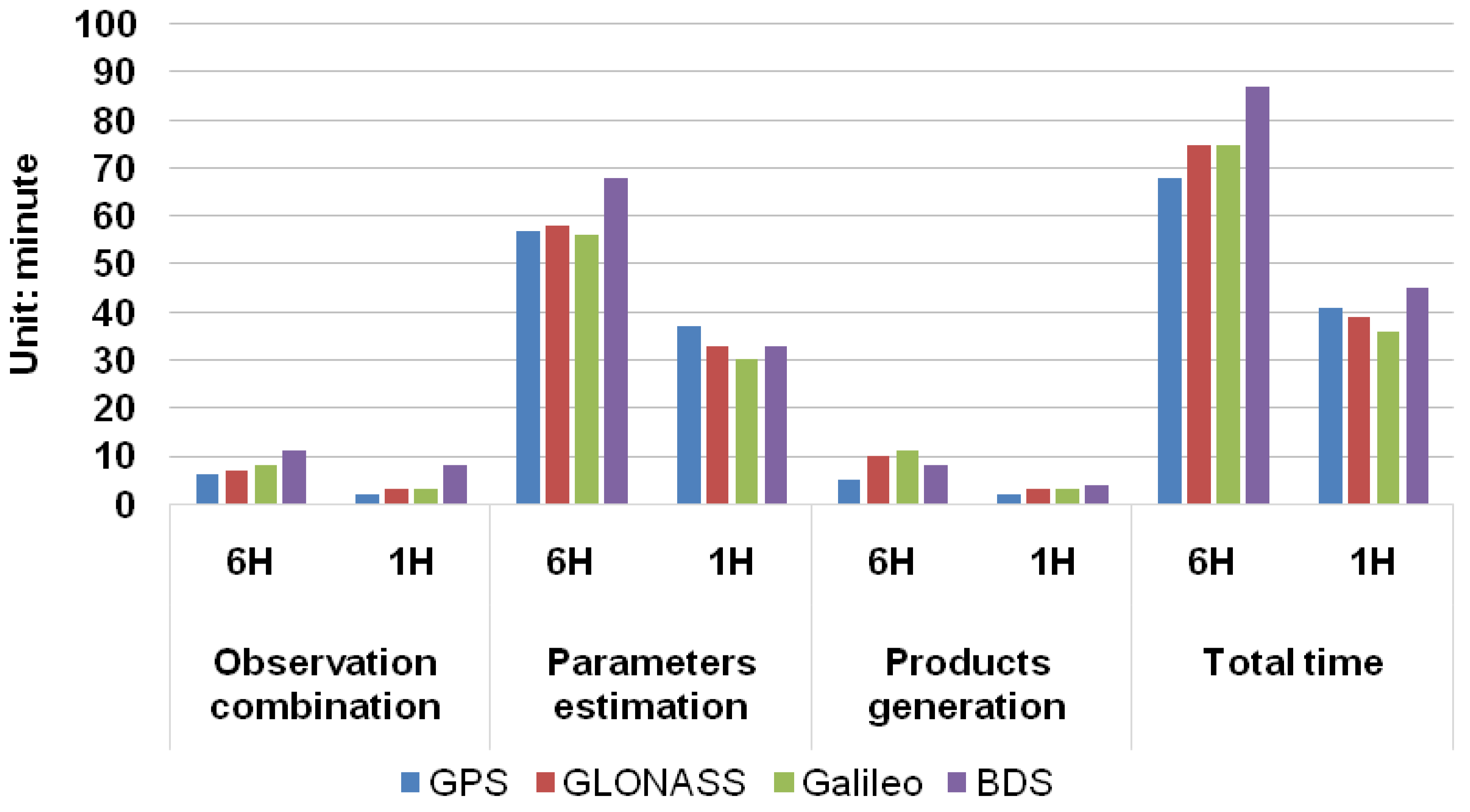
The total time consumption of the procedure of 6H ultra-rapid products was about 90 min, which may not satisfy the requirement of users. Thus, in order to improve the computational efficiency, the procedure of 1H products was improved by the optimized CSPT method for product generation. The quality control of observation and navigation data was also improved for 1H products to reduce the iteration of the least square parameter estimation. The time consumption of the 6H and 1H product generation procedure for GNSS is shown in Figure 4. We can see the procedure mainly includes three steps: observation combination, parameters estimation, and products generation. The total time consumption of 1H is 41, 39, 36, and 45minutes for GPS, GLONASS, Galileo, and BDS, which are less than 6H for three steps, respectively. The efficiency of 1H was improved by 40%, 48%, 52%, and 48% for GPS, GLONASS, Galileo, and BDS, with respect to 6H, respectively. Thus, the improved method of 1H shows a promising application for real-time or near-real-time applications.
Figure 4 shows that the latency is no more than 2 h for 6H, and 1hour for 1H. Moreover, the available prediction session of the orbit and clock products is 1st–8th hour for 6H and 1st–2nd hour for 1H. Thus, in this study, the accuracy and precision of the observed and 1st–8th and 1st–2nd prediction sessions for 6H and 1H products are analyzed and discussed in detail.
3.2. Accuracy Analysis of Different Methods for Orbit Prediction
In order to access and analyze the performance of the 6H and 1H products, the orbit and clock products from another source with high accuracy should be chosen as a reference. The IGS provided final combined products, which are well known with high accuracy. Thus, the IGS final combined products can be used as the reference to access accuracy of the GPS orbit and clock and GLONASS orbit. However, the combined orbit and clock products for Galileo and BDS are not provided by IGS yet. Fortunately, several ACs provided the GNSS products for MGEX. The orbit and clock products from GFZ have been assessed and showed better performance [8,14]. Thus, in this study, GFZ’s orbit and clock products are used as the reference to access the accuracy of orbit and clock for Galileo and BDS, and for GLONASS, because the combined GLONASS clock products is not provided by IGS [27].
Lutz et al. (2014) analyzed the impact of the one-day and three-day arc length on orbit accuracy. Li et al. (2019) assessed orbit accuracy of the two-day ultra-rapid solutions. Ma et al. (2017) analyzed the accuracy of the 25-h solution. Their results show the long-arc solutions will improve the accuracy and disclosures of the orbit [8,11,28]. However, the long-arc solutions will increase time consumption, which means the products will not be provided to users on time. Thus, a new method to generate the prediction session of the orbit is discussed in this section, before accessing the accuracy of 6H and 1H products.
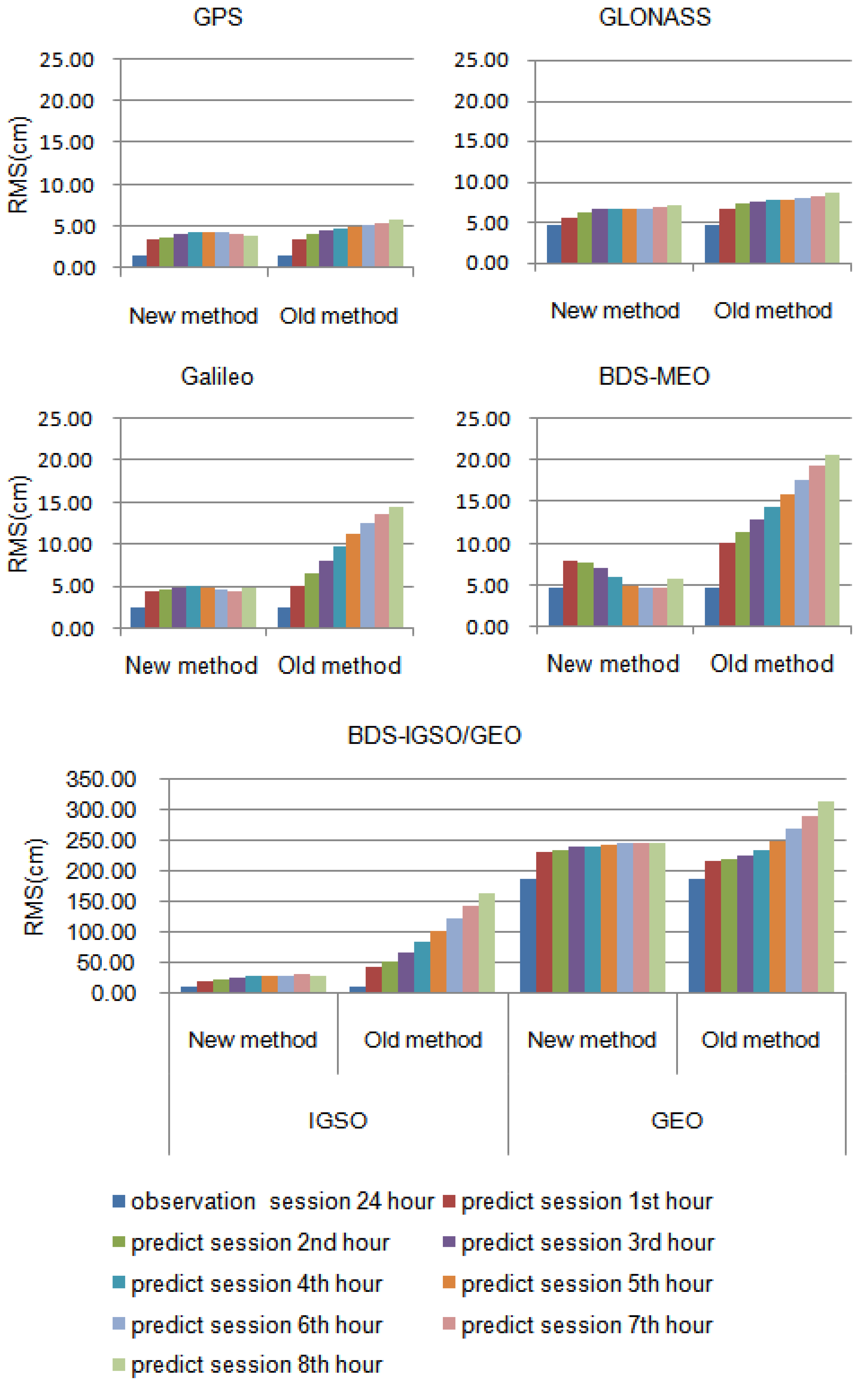
Obviously, the accuracy and the computational efficiency of the orbit and clock products is an important issue for users, which should be considered together, especially for ultra-rapid products. The new method is addressed for integrating the forecast orbit by the fitted orbit, from 24 h, and adjacent afore 24 h-orbits, which were determined by observation data values. The results are analyzed with respect to the old method, which integrated forecast orbits from only 24-h orbits.
Figure 5 and Table 2 show the accuracy of the orbit for the new and old method for GPS/GLONASS/Galileo/BDS from day of the year (DOY) 041st to 043rd in the year 2019, with respect to IGS/MGEX products. We can see the accuracy of the 24-h observation orbit is close between new and old methods. The root mean square (RMS) of GPS prediction orbit in along, cross, and radial directions is from 3.5 cm to 4.4 cm for the 1st–8th prediction hour for the new method, which is improved from 9% to 32% versus the old method. The RMS of the GLONASS prediction orbit is from 5.7 cm to 7.1 cm for the new method, which is improved from 13% to 19% relative to the old method. The RMS of the Galileo prediction orbit is from 4.4 cm to 5.0 cm for the new method. The accuracy for the new method is improved from 12% to 67% relative to the old method, which shows an obvious improvement. Similar to Galileo, a distinct improvement can be seen from the BDS prediction orbit for the new method, especially for MEO and IGSO. The RMS is from 4.7 to 8 cm for the BDS MEO prediction orbit for the new method, which is improved from the 20% to 73% versus the old method. Moreover, the RMS is from 18 cm to 28 cm for prediction BDS IGSO for the new method, improved from 54% to 83% versus the old method. However, accuracy of BDS GEO prediction orbit for the new method is close to the old method. Thus, the results show the new method can improve the accuracy of the prediction GNSS orbit, especially for Galileo and BDS.
3.3. Assessment of 6H and 1H Orbit Products
The accuracy of 6H and 1H orbit products for GPS, GLONASS, Galileo, and BDS is analyzed by comparing the reference productions from IGS/MGEX. This method compares the orbit positions between our orbit products with reference orbits at a 15 min sampling in radial, along-tracking, and cross-tracking direction, with seven-parameter Helmet rotation transformation. Moreover, the results are expressed as mean 1DRMS values over the three components for different types of GNSS satellites, such as MEO, IGSO, and GEO, respectively.
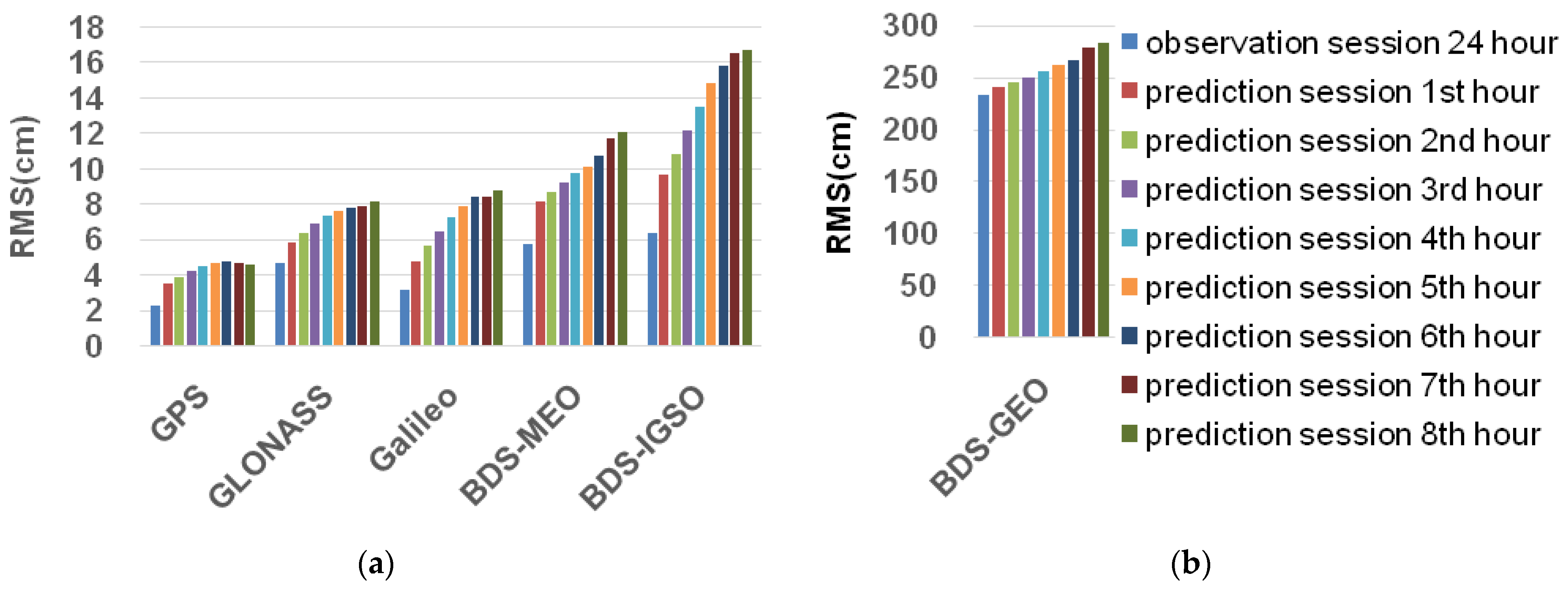
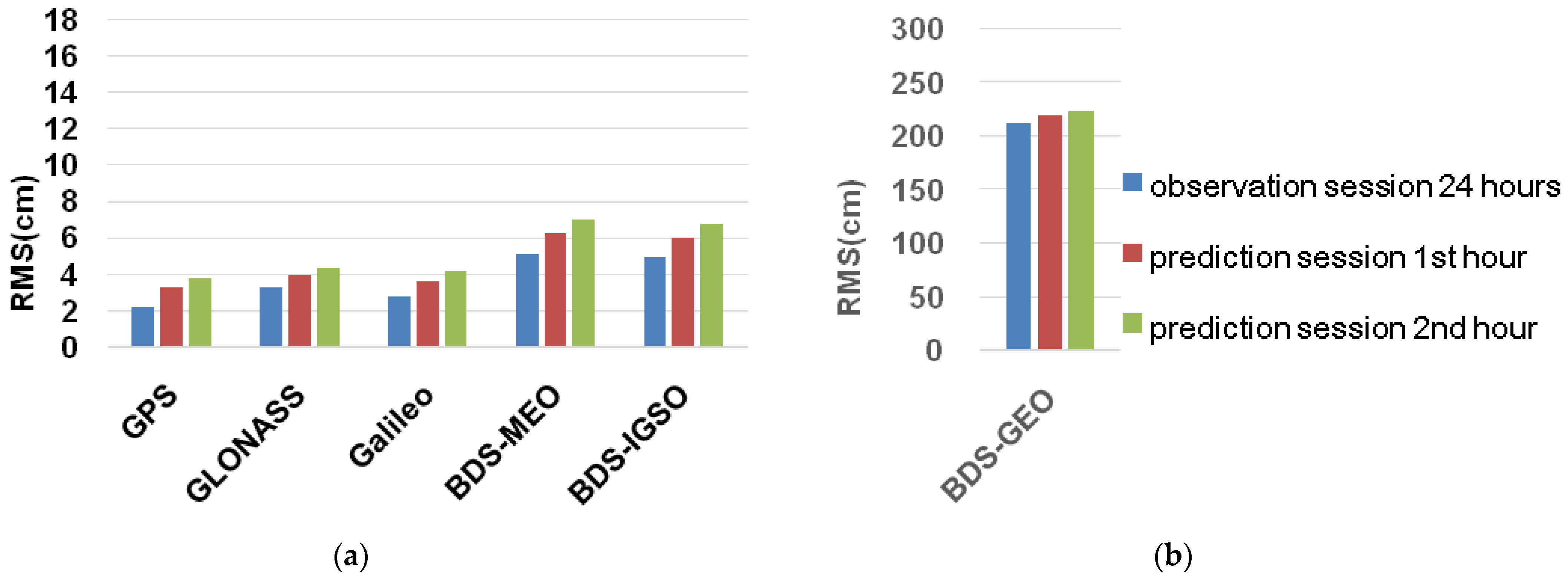
Figure 6 and Figure 7 show the average RMS of the orbit difference including the observation and prediction session for 6H and 1H orbit with respect to the reference orbit for GPS, GLONASS, Galileo, and BDS over the period from the 041st to 050th days of the year in 2019 (from 10 February 2019 to 19 February 2019).
For GPS satellites, the average RMS of 6H was about 2 cm for the observation session. However, the RMS of the prediction orbit was from 3.5 to 4.7 cm for the 1st–8th hour prediction session. The accuracy of prediction shows a diminishing trend, with the prediction hour session increasing. The mean RMS of observation and 1st–2nd hour prediction session was 2.2 cm and 3.3–3.8 cm for 1H, which is better than 6H. Moreover, the higher renewal rate of 1H will provide the better accuracy of 1H orbit products, which can be provided to users during the 3rd–8th prediction hours of 6H.
For GLONASS satellites, the average RMS for 6H was less than 4.7 cm for the observation session, while the RMS of the prediction session was from 5.8 to 8.1 cm, which is worse than GPS, due to the difficulty in GLONASS ambiguity fixing, and the bad tracking site distributed in some places, such as the Russian area. Moreover, the average RMS for 1H was about 3.2 cm and 3.9–4.3 cm for observation, and 1st–2nd hour prediction sessions, which is better than 6H. The high updated rate, recently updated observation data, and the improved strategy may benefit the 1H orbit.
For Galileo satellites, the mean RMS of 6H was about 3.2 cm and 4.7–8.7 cm for observation and 1st–8th hour prediction session. While the mean RMS of 1H was about 2.8 cm and 3.6-4.2 cm for observation and 1st–2nd hour prediction session.
For BDS satellites, the average RMS of 6H observation and 1st–8th hour prediction session for MEO satellites was about 5.7 cm and 8–12 cm, which is better than that of IGSO and GEO because of the limitation of tracking station distribution for the latter. While the mean RMS of 1H was about 5 cm and 6–7 cm for observation and 1st–2nd hour prediction session. The BDS–GEO shows the worst accuracy mainly due to the poor distribution of ground stations and limited constellation.
In general, we can see the mean RMS of the observation session for 6H orbit was comparative to 1H. However, the accuracy of 6H decreased when the prediction hour session increased. The GPS shows the orbit productions with best accuracy, followed by GLONASS, Galileo, and BDS-MEO/IGSO/GEO. The limited station distribution for some areas for GLONASS/Galileo/BDS, the improper attitude model, and the SRPs model used for Galileo/BDS and the PCC, without better accuracy for BDS, may decrease the accuracy of GLONASS/Galileo/BDS. However, the RMS of the 1H prediction orbit was better than 6H due to the improved strategy and the latest updated observation data being used to generate the productions for GPS/GLONASS/Galileo/BDS.
Table 3 shows that the accuracy of 1H GNSS orbits improved about 1%, 31%, 13%, 11%, 23%, 9% for the observation session, and 18%, 43%, 45%, 34%, 53%, 15% for the prediction session of GPS, GLONASS, Galileo, BDS MEO, IGSO, and GEO orbit, relative when compared with reference products from IGS/MGEX, which shows encouraging prospects for real-time or near-real-time studies and applications.
3.4. Assessment of 6H and 1H Clock Products
In this study, the GNSS clock was estimated, relatively, with respect to a reference clock. Thus, the clock bias must be removed before comparing with the reference products from IGS/MGEX. A satellite clock of GPS is selected as the reference clock because GLONASS/Galileo/BDS are coupled with GPS in the running threads. Then the difference between other satellite clocks and the reference clock for each epoch are calculated to remove the clock bias. Moreover, the RMS and SD of the differences between our hourly clock productions and reference clock products from IGS/MGEX are summarized to assess the quality of the clock.
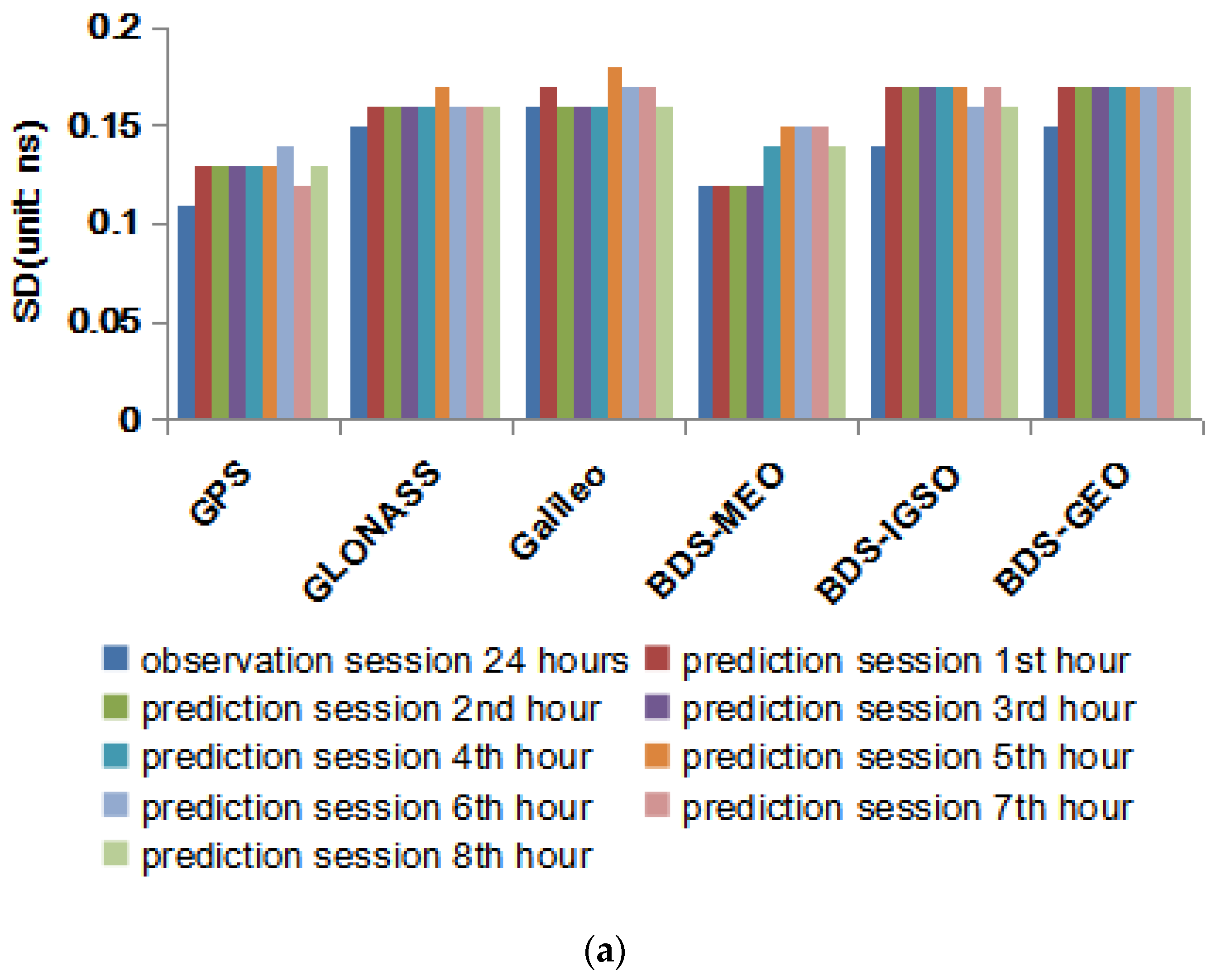
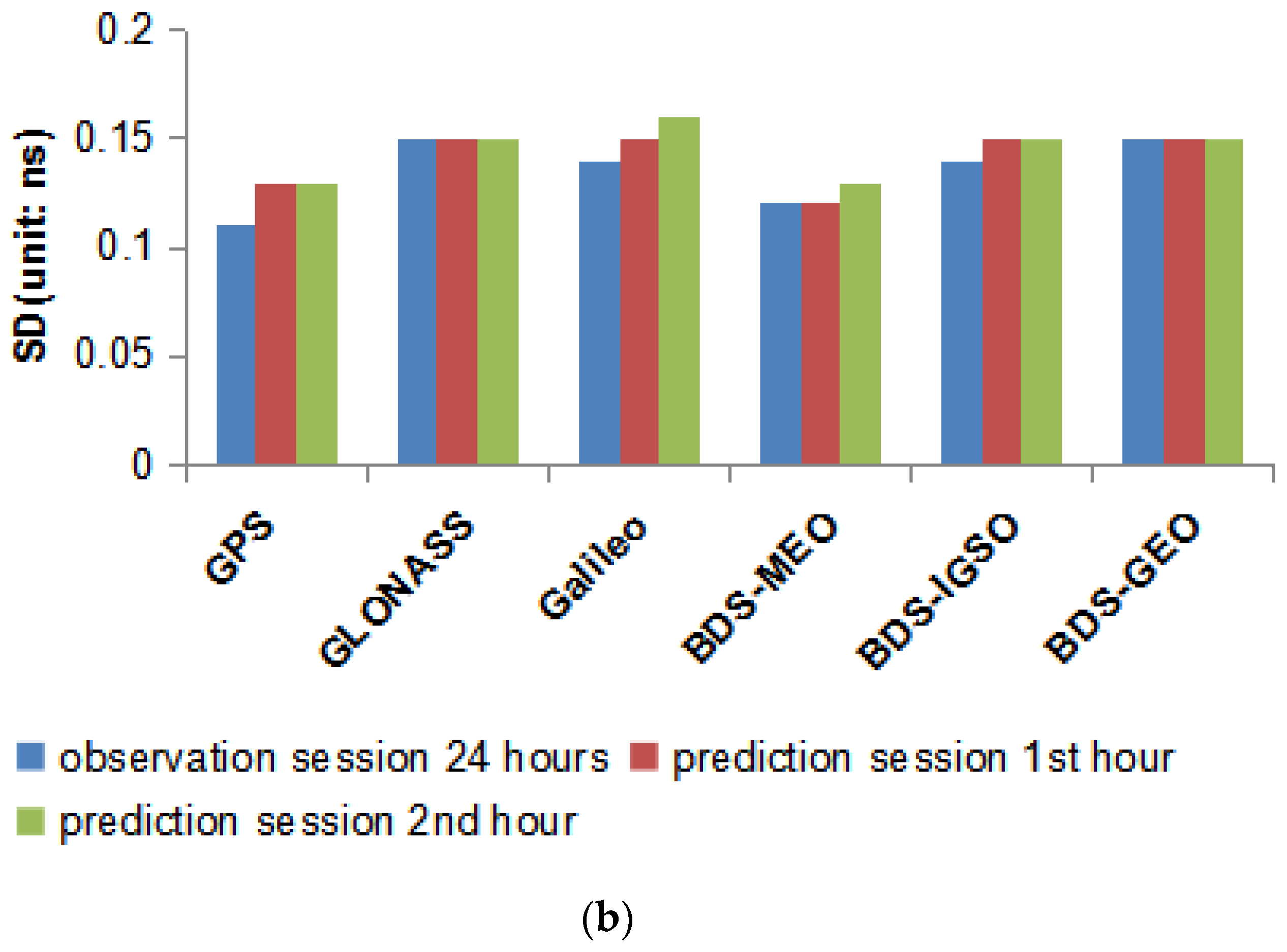
Figure 8 shows the average SD values for 6H (top chart) clock versus reference products. The mean SD of the observation session for GNSS satellites are no more than 0.16 ns. The GPS clock shows the best accuracy, followed by BDS–MEO, GLONASS, and Galileo. Moreover, the SD of BDS MEO are better than IGSO/GEO, for more global tracking stations available for MEO. While the SD of the GNSS prediction clock is less than 0.18 ns, which is a little worse than the observation session, but can be available to users. The mean SD for 1H (bottom chart) clock is less than 0.16 ns for the observation session, or even the 1st–2nd hour prediction session, which benefits from the higher updated rate and shorter prediction session, and shows better performance than 6H.
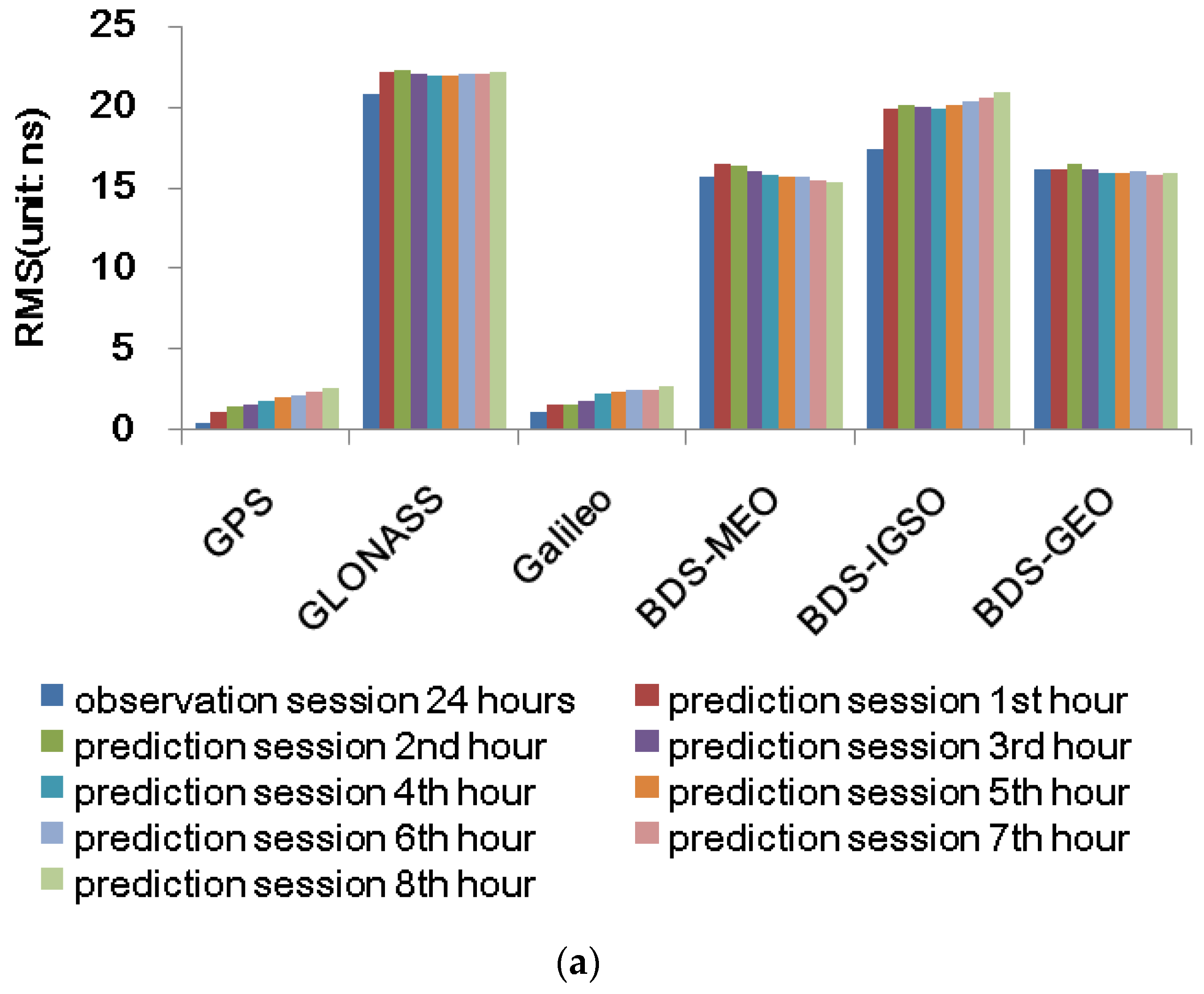
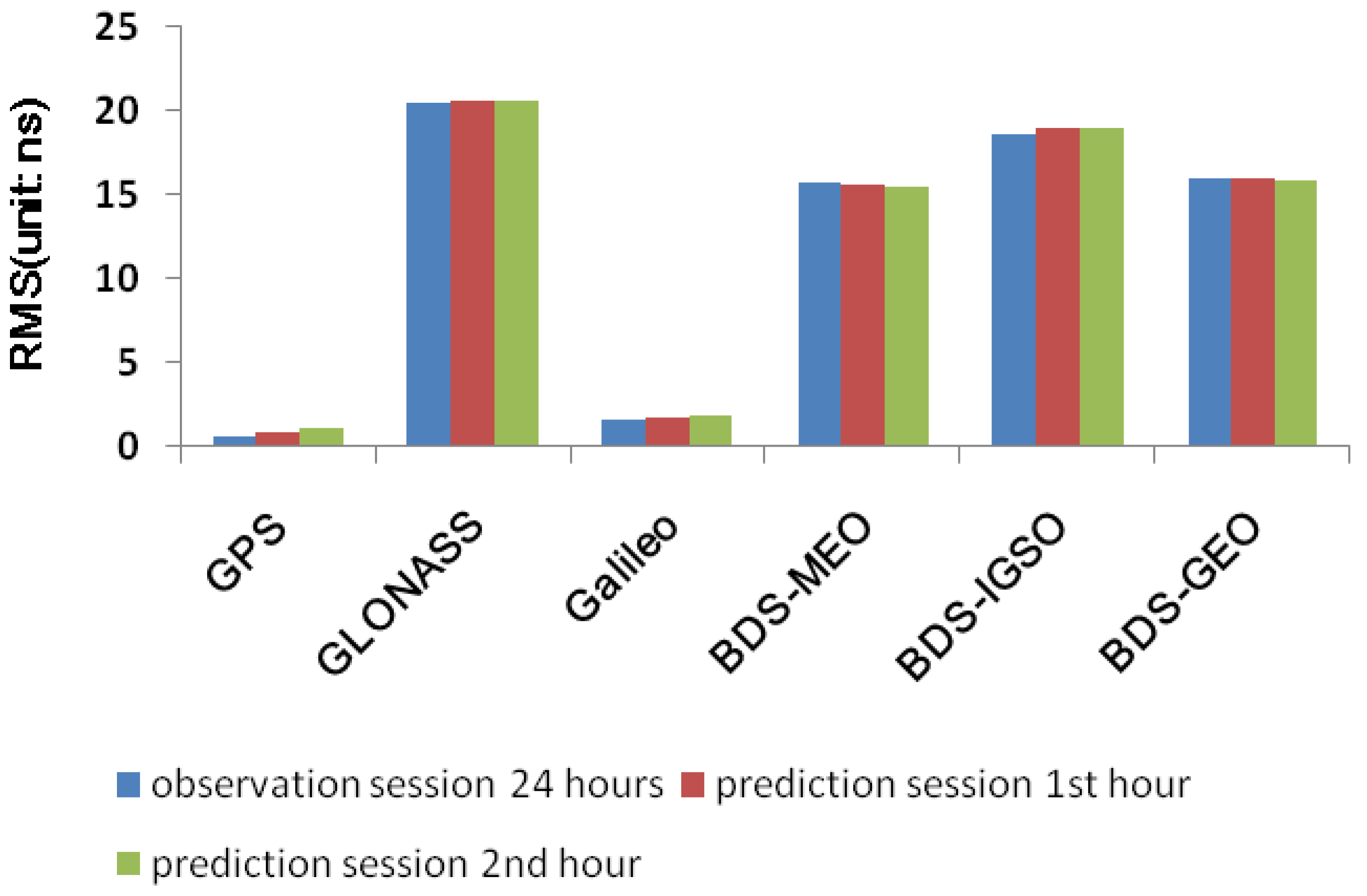
Figure 9 shows the mean RMS of 6H and 1H for GNSS clock with respect to reference clock products. The mean RMS of 6H for GPS is about 0.42 ns and 1.16–2.58 ns for observation and 1st–8th hour prediction session, which also shows better accuracy followed with Galileo, BDS, and GLONASS. The RMS of the prediction session shows anincreasing trend for GPS and Galileo, which means the accuracy decreases when the prediction hour augments. The mean RMS of BDS GEO clock is worse because of the station distribution limit and complicated satellite constellation, no better phase center correction (PCC) available, and the improper SRP model. The RMS of the GLONASS is the worst due to the possible bias caused from the FDMA signal transmit mechanism and the float ambiguity solutions. The mean RMS for the 1H clock is similar to the 6H, but the advantage of 1H is that it can provide the users clock products with higher updated rates, which is better than the poor accuracy of the broadcast clock and can be used as initial values for real-time or near-real-time applications.
4. Summary and Conclusions
Due to the demand of hourly ultra-rapid GNSS products with less latency, high accuracy, and updated rates for real-time or near-real-time studies and applications, we mainly discussed a new strategy and method for generating 6-hourly and 1-hourly GNSS orbit and clock products. The new method, which combined serial and parallel threads (CSPT), is studied in this contribution, and is different from previous researches. A new method of orbit prediction is also introduced and shows better accuracy compared to the old method. The computational efficiency, accuracy, and precision of the new strategy and method are discussed and analyzed in detail.
The 6H and 1H GNSS orbit products were compared with reference products, with high accuracy from IGS/MGEX. Generally, the RMS of the observation session for the 6H orbit is comparative to 1H. However, the accuracy of 6H decreases when the prediction session increases. GPS shows the best accuracy, followed by GLONASS, Galileo, and BDS-MEO/IGSO/GEO. Moreover, the accuracy of 1H orbit is improved about 1%, 31%, 13%, 11%, 23%, 9% for the observation sessionand18%, 43%, 45%, 34%, 53%, 15% for the prediction session of GPS, GLONASS, Galileo, BDS MEO, IGSO, and GEO, relative to 6H orbit.
The accuracy of 6H and 1H clock, with respect to reference clock products, are also analyzed. The mean SD of the observation session for the 6H clock is no more than 0.16 ns, and the GPS shows the best accuracy, followed by BDS, GLONASS, and Galileo. The mean SD of the GNSS prediction clock is less than 0.18 ns, which is a little worse than the SD of the observation session. The mean SD for the 1H clock is less than 0.16 ns for the observation session or even the 1st–2nd hour prediction session, which benefits from the higher updated rate and shorter prediction session.
The 1H orbit and clock productions show better accuracy and precision relative to 6H. Some problems appearing in stations or satellites can be found and solved earlier and by the 1H procedure, which is useful for user applications.
The results show the feasibility of the optimized CSPT method for GNSS hourly ultra-rapid orbit and clock products. The accuracy of the 6H and 1H orbit and clock verify the availability and reliability of the hourly ultra-rapid products, which can be used for real-time or near-real-time applications. Moreover, the CSPT method caneasily avoid the problems caused by a bad satellite or station, and it improves the computational efficiency, continuity, and stability of ultra-rapid productions. Thus, the CSPT method shows encouraging prospects for better performance and deserves wide application.
Author Contributions
Conceptualization, Q.C. and S.S.; methodology, Q.C.; software, Q.C.; validation, W.Z. and Q.C.; formal analysis, S.S.; investigation, Q.C. and W.Z.; resources, S.S. and Q.C.; data curation, Q.C.; writing—original draft preparation, Q.C.; writing—review and editing, S.S. and W.Z.; visualization, Q.C.; supervision, S.S.; project administration, S.S.; funding acquisition, Q.C. and S.S. All authors have read and agreed to the published version of the manuscript.
Funding
This research was funded by ZFS (Y9E0151M26) and National Natural Science Foundation of China (No. 12073063, 11403083).
Data Availability Statement
Not applicable.
Acknowledgments
Thanks to IGS/MGEX, iGMAS, and CMONOC for providing the data and products to support this study. The reviewers and editors of this paper are also appreciated by the authors.
Conflicts of Interest
The authors declare no conflict of interest.
Appendix A. The POD Processing by Combined Serial and Parallel Threads (CSPT)
The undifferenced (UD) observation model for code pseudorange (P) and carrier phase observations can be showed by distance, as follows:
where s, r, and i (i = 1, 2) are on half of satellites, receivers, and frequencies, respectively. is the geometric distance between satellite and receiver, and denote satellite and receiver clock bias, respectively. c is light velocity. and refer to receiver and satellite code bias at frequency i. and represent the mapping function and zenith tropospheric delay at receiver position. denotes the ionospheric delay from receiver to satellite. is the wave length for frequency i. , and illuminate the uncalibrated phase delays (UPDs) for receivers and satellites. is the integer ambiguity between receiver and satellite pairs at frequency i. and denote the sum of the noise and other un-modeled corrections. Other corrections, such as phase center offset (PCO), phase center variations (PCV), and ocean tide loading, etc., are corrected by models (introduced in Section 2).
In order to eliminate the low order ionospheric delays, the ionosphere-free (IF), combined between double frequencies, are applied in this contribution. It should be noted that the time consumption would increase dramatically if four satellite navigation systems were combined to estimate orbit and clock parameters. Four threads were running at the same time to generate the orbit and clock products for GPS, GLONASS, Galileo, and BDS by distributed parallelism mode, as Formulas (3)–(6) shows. Formulas (4)–(6) also show GLONASS, Galileo, and BDS are coupled with GPS to improve the accuracy of the orbit and clock products for GLONASS, Galileo, and BDS, respectively.
where and refer to observed minus computed values for pseudorange and phase IF combination observations. denotes the unit vector of receiver-satellite direction. is the satellite initial orbit state vector, including initial position, velocity, and five solar radiation pressure parameters. is on behalf of state transition matrix from initial to t. is position vector of receiver. G, R, E and C are the abbreviation of GPS, GLONASS, Galileo and BDS. S represents the satellite system G or the couple combination of the between R/E/C with G, respectively. The state vector X ofestimated parameters include the initial orbit state vector , the receiver position , the satellite clock bias , the receiver clock bias , the ZTD, the ERP parameters , the phase ambiguities , and the inter system bias (ISB) or inter-frequency bias (IFB) relative to GPS biases , and . and denote the IF combination noise and other un-modeled corrections for pseudorange and phase, respectively.
In order to remain the consistent of space and time datumof the orbit and clock products for GPS, GLONASS, Galileo and BDS, the same station network are applied for four CSPT threads showed by formula 3-6, and the coordinate of the IGS/MGEX stations are retrieved from IGS weekly updated solution independent exchange (SINEX) format files and strongly constrained. Moreover, a reference clock is fixed when estimated the satellite and receiver clock biases in order to remain the same time reference, and then the estimated satellite and receiver clock biases subtract another reference clock bias to eliminate the clock bias difference in these four threads. The reference clock should be connected with hydrogen atomic clock and showed better performance, such as ALGO, PTBB, WTZR, NRC1, PIE1 or ONSA.
where and denote the satellite and receiver clock bias which eliminate the clock bias difference, respectively. is the clock bias of the reference receiver.
The orbit and clock parameters are estimated through batch least square (LSQ) mode, in which linear algebra package (LAPACK) optimized function libraries are applied to decompose and inverse the normal matrix. The methods of generating prediction orbit and clock are introduced in Section 2.
References
- Cai, H.; Chen, K.; Xu, T.; Chen, G. The iGMAS Combined Products and the Analysis of Their Consistency. China Satell. Navig. Conf. 2015, 342, 213–226. [Google Scholar] [CrossRef]
- Montenbruck, O.; Steigenberger, P.; Prange, L.; Deng, Z.; Zhao, Q.; Perosanz, F.; Romero, I.; Noll, C.; Stürze, A.; Weber, G.; et al. The Multi-GNSS Experiment (MGEX) of the International GNSS Service (IGS)—Achievements, prospects and challenges. Adv. Space Res. 2017, 59, 1671–1697. [Google Scholar] [CrossRef]
- Yang, Y.; Li, J.; Wang, A.; Xu, J.; He, H.; Guo, H.; Shen, J.; Dai, X. Preliminary assessment of the navigation and positioning performance of BeiDou regional navigation satellite system. Sci. China Earth Sci. 2013, 57, 144–152. [Google Scholar] [CrossRef]
- Yang, Y.; Xu, Y.; Li, J.; Yang, C. Progress and performance evaluation of BeiDou global navigation satellite system: Data analysis based on BDS-3 demonstration system. Sci. China Earth Sci. 2018, 61, 614–624. [Google Scholar] [CrossRef]
- Oh, H.; Park, E.; Lim, H.C.; Park, C. Orbit Determination of Korean GEO Satellite Using Single SLR Sensor. Sensors 2018, 18, 2847. [Google Scholar] [CrossRef] [Green Version]
- Wang, K.; Chen, P.; Zaminpardaz, S.; Teunissen, P.J.G. Precise regional L5 positioning with IRNSS and QZSS: Stand-alone and combined. GPS Solut. 2019, 23. [Google Scholar] [CrossRef] [Green Version]
- Jiao, W.; Ding, Q.; Li, J.; Lu, X.; Feng, L.; Ma, J.; Chen, G. Monitoring and Assessment of GNSS Open Services. J. Navig. 2011, 64, S19–S29. [Google Scholar] [CrossRef]
- Li, X.X.; Chen, X.H.; Ge, M.R.; Schuh, H. Improving multi-GNSS ultra-rapid orbit determination for real-time precise point positioning. J. Geod. 2019, 93, 45–64. [Google Scholar] [CrossRef]
- Prange, L.; Orliac, E.; Dach, R.; Arnold, D.; Beutler, G.; Schaer, S.; Jäggi, A. CODE’s five-system orbit and clock solution—The challenges of multi-GNSS data analysis. J. Geod. 2016, 91, 345–360. [Google Scholar] [CrossRef] [Green Version]
- Johnston, G.; Riddell, A.; Hausler, G. The International GNSS Service. In Springer Handbook of Global Navigation Satellite Systems; Teunissen, P.J.G., Montenbruck, O., Eds.; Springer International Publishing: Cham, Switzerland, 2017; Volume 1, pp. 967–982. [Google Scholar] [CrossRef]
- Ma, H.Y.; Zhao, Q.L.; Xu, X.L. A New Method and Strategy for Precise Ultra-Rapid Orbit Determination. China Satell. Navig. Conf. 2017, 439, 191–205. [Google Scholar] [CrossRef]
- Li, X.X.; Zus, F.; Lu, C.X.; Dick, G.; Ning, T.; Ge, M.R.; Wickert, J.; Schuh, H. Retrieving of atmospheric parameters from multi-GNSS in real time: Validation with water vapor radiometer and numerical weather model. J. Geophys. Res. Atmos. 2015, 120, 7189–7204. [Google Scholar] [CrossRef] [Green Version]
- Choi, K.K.; Ray, J.; Griffiths, J.; Bae, T.-S. Evaluation of GPS orbit prediction strategies for the IGS Ultra-rapid products. GPS Solut. 2012, 17, 403–412. [Google Scholar] [CrossRef]
- Guo, J.; Xu, X.L.; Zhao, Q.L.; Liu, J.N. Precise orbit determination for quad-constellation satellites at Wuhan University: Strategy, result validation, and comparison. J. Geod. 2016, 90, 143–159. [Google Scholar] [CrossRef]
- Wu, J.T.; Wu, S.C.; Hajj, G.A.; Bertiger, W.I.; Lichten, S.M. Effects of Antenna Orientation on GPS Phase. Manuscr. Geod. 1993, 18, 91–98. [Google Scholar]
- Lyard, F.; Lefevre, F.; Letellier, T.; Francis, O. Modelling the global ocean tides: Modern insights from FES2004. Ocean Dyn. 2006, 56, 394–415. [Google Scholar] [CrossRef]
- Ge, M.; Gendt, G.; Dick, G.; Zhang, F.P. Improving carrier-phase ambiguity resolution in global GPS network solutions. J. Geod. 2005, 79, 103–110. [Google Scholar] [CrossRef]
- Montenbruck, O.; Schmid, R.; Mercier, F.; Steigenberger, P.; Noll, C.; Fatkulin, R.; Kogure, S.; Ganeshan, A.S. GNSS satellite geometry and attitude models. Adv. Space Res. 2015, 56, 1015–1029. [Google Scholar] [CrossRef] [Green Version]
- Schmid, R.; Dach, R.; Collilieux, X.; Jaggi, A.; Schmitz, M.; Dilssner, F. Absolute IGS antenna phase center model igs08.atx: Status and potential improvements. J. Geod. 2016, 90, 343–364. [Google Scholar] [CrossRef] [Green Version]
- Saastamoinen, J. Atmospheric Correction for the Troposphere and Stratosphere in Radio Ranging Satellites. Use Artif. Satell. Geod. 2013, 247–251. [Google Scholar] [CrossRef]
- Chen, Q.M.; Song, S.L.; Heise, S.; Liou, Y.A.; Zhu, W.Y.; Zhao, J.Y. Assessment of ZTD derived from ECMWF/NCEP data with GPS ZTD over China. GPS Solut. 2011, 15, 415–425. [Google Scholar] [CrossRef]
- Boehm, J.; Niell, A.; Tregoning, P.; Schuh, H. Global Mapping Function (GMF): A new empirical mapping function based on numerical weather model data. Geophys. Res. Lett. 2006, 33. [Google Scholar] [CrossRef] [Green Version]
- Boehm, J.; Schuh, H. Vienna mapping functions in VLBI analyses. Geophys. Res. Lett. 2004, 31. [Google Scholar] [CrossRef]
- Boehm, J.; Werl, B.; Schuh, H. Troposphere mapping functions for GPS and very long baseline interferometry from European Centre for Medium-Range Weather Forecasts operational analysis data. J. Geophys. Res. Solid Earth 2006, 111. [Google Scholar] [CrossRef]
- Bohm, J.; Hobiger, T.; Ichikawa, R.; Kondo, T.; Koyama, Y.; Pany, A.; Schuh, H.; Teke, K. Asymmetric tropospheric delays from numerical weather models for UT1 determination from VLBI Intensive sessions on the baseline Wettzell-Tsukuba. J. Geod. 2010, 84, 319–325. [Google Scholar] [CrossRef]
- Zhou, W.; Huang, C.; Song, S.; Chen, Q.; Liu, Z. Characteristic Analysis and Short-Term Prediction of GPS/BDS Satellite Clock Correction. China Satell. Navig. Conf. 2016, 390, 187–200. [Google Scholar] [CrossRef]
- Noll, C.E. The crustal dynamics data information system: A resource to support scientific analysis using space geodesy. Adv. Space Res. 2010, 45, 1421–1440. [Google Scholar] [CrossRef] [Green Version]
- Lutz, S.; Beutler, G.; Schaer, S.; Dach, R.; Jäggi, A. CODE’s new ultra-rapid orbit and ERP products for the IGS. GPS Solut. 2014, 20, 239–250. [Google Scholar] [CrossRef] [Green Version]
Figure 1.
Distribution of the global tracking stations used to generate hourly ultra-rapid orbit and clock global navigation satellite system (GNSS) products. The blue circles represent the stations, which can track American Global Positioning System (GPS) satellites; the green circles represent the stations tracking Ruassian Global’naya Navigatsionnaya Sputnikova Sistema (GLONASS); the yellow circles represent the stations tracking European Union’s Galileo, and the red circles represent the stations tracking Chinese BeiDou navigation satellite system (BDS) satellites.

Figure 2.
Slide window for hourly ultra-rapid obit and clock products generation.

Figure 3.
Data processing flow chart of the combined serial and parallel threads (CSPT) method for hourly orbit and clock products.
Figure 3.
Data processing flow chart of the combined serial and parallel threads (CSPT) method for hourly orbit and clock products.

Figure 4.
Computational efficiency of 6H and 1H products for GPS/GLONASS/Galileo/BDS. The 6H and 1H are on behalf of 6-hourly and 1-hourly products, respectively.
Figure 4.
Computational efficiency of 6H and 1H products for GPS/GLONASS/Galileo/BDS. The 6H and 1H are on behalf of 6-hourly and 1-hourly products, respectively.

Figure 5.
Average root mean square (RMS) in along, cross, and radial directions of differences between 6-hourlyorbit products generated by the new and old method and IGS/MGEX final products for 24-h observation session and the 1st–8th hour prediction session.
Figure 5.
Average root mean square (RMS) in along, cross, and radial directions of differences between 6-hourlyorbit products generated by the new and old method and IGS/MGEX final products for 24-h observation session and the 1st–8th hour prediction session.

Figure 6.
Average RMS of 6-hourly GNSS ultra-rapid orbit products with respect to IGS/MGEX final products for 24-h observation session and 1st–8th prediction session. (a) shows RMS of the MEO orbit for GPS/GLONASS/Galileo, and MEO/IGSO orbit for BDS, (b) displays RMS of GEO orbit for BDS for the observation session and prediction session.

Figure 7.
Average RMS of 1-hourly GNSS ultra-rapid orbit products with respect to IGS/MGEX final products for 24-h observation session and 1st–2nd prediction session. (a) shows RMS of the MEO orbit for GPS/GLONASS/Galileo, and MEO/IGSO for BDS, (b) displays RMS of GEO orbit for BDS for the observation session and prediction session.

Figure 8.
Average SD of 6-hourly (a) and 1-hourly (b) GNSS clock versus reference products from IGS/MGEX.
Figure 8.
Average SD of 6-hourly (a) and 1-hourly (b) GNSS clock versus reference products from IGS/MGEX.


Figure 9.
Average RMS of 6-hourly (a) and 1-hourly (b) GNSS clock versus reference products from IGS/MGEX.
Figure 9.
Average RMS of 6-hourly (a) and 1-hourly (b) GNSS clock versus reference products from IGS/MGEX.


Table 1.
Strategy for hourly GNSS products generation.
| GPS | GLONASS | Galileo | BDS | |
| Thread | GPS | GLONASS+GPS | Galileo+GPS | BDS+GPS |
| Undifferenced ionosphere-free combination | GPS: L1,L2 | GLONASS: L1,L2 | Galileo: E1,E5a | BDS: B1,B2 |
| GPS: L1,L2 | GPS: L1,L2 | GPS: L1,L2 | ||
| Elevation angle cutoff | 7 degrees | |||
| Sampling interval | 450 s for 6-hourly updated products | |||
| 600 s for 1-hourly updated products | ||||
| ISB/IFB | Estimated as constant | |||
| Satellite clock error | Estimate every sampling interval relative to reference clock | |||
| Receiver clock error | Estimate every sampling interval relative to reference clock | |||
| A receiver clock fixed as a time reference (such as ALGO, PTBB, WTZR, NRC1, PIE1, ONSA) | ||||
| Orbits | Estimated with 5 parameters for solar radiation pressure modeling | |||
| station displacement | Solid earth tide, pole tide, ocean tide loading | |||
| Earth gravity | EGM 12X12 | |||
| RHC phase rotation correction | Phase wind-up applied | |||
| Ambiguities | Fixed | |||
| Satellite phase center corrections | igs14.atx from IGS | PCO/PCV for BDS-2 [14] | ||
| Station phase center corrections | igs14_absolute.atx from IGS | |||
| Tropospheric delay | Initial ZTD model: Saastamoinen model | |||
| Mapping function: GMF | ||||
| Interval: 1-h for ZTD, 12-h for gradient | ||||
| ERP | Initial value: downloaded from IERS rapid solution | |||
| Constrain: strong constrain | ||||
| Reference frame | ITRF 2014 | |||
Table 2.
Relatively improved accuracy for the new method relative to the old method.
| Session | GPS | GLONASS | Galileo | BDS | |||
|---|---|---|---|---|---|---|---|
| MEO | MEO | MEO | MEO | IGSO | GEO | ||
| Observation session | 24 h | 0% | 0% | 0% | 0% | 0% | 0% |
| Prediction session | 1st hour | 0% | 15% | 12% | 20% | 54% | −7% |
| 2nd hour | 9% | 14% | 28% | 32% | 59% | −7% | |
| 3rd hour | 9% | 13% | 41% | 46% | 64% | −6% | |
| 4th hour | 9% | 15% | 49% | 58% | 69% | −3% | |
| 5th hour | 13% | 14% | 57% | 69% | 73% | 3% | |
| 6th hour | 16% | 16% | 64% | 74% | 77% | 9% | |
| 7th hour | 22% | 18% | 67% | 76% | 80% | 15% | |
| 8th hour | 32% | 19% | 67% | 73% | 83% | 21% | |
Table 3.
Improved accuracy of 1H relative to 6H orbit for observation and prediction session.
| Session | GPS | GLONASS | Galileo | BDS–MEO | BDS–IGSO | BDS–GEO |
|---|---|---|---|---|---|---|
| MEO | MEO | MEO | MEO | IGSO | GEO | |
| Observation | 1% | 31% | 13% | 11% | 23% | 9% |
| Prediction | 18% | 43% | 45% | 34% | 53% | 15% |
Publisher’s Note: MDPI stays neutral with regard to jurisdictional claims in published maps and institutional affiliations. |
© 2021 by the authors. Licensee MDPI, Basel, Switzerland. This article is an open access article distributed under the terms and conditions of the Creative Commons Attribution (CC BY) license (http://creativecommons.org/licenses/by/4.0/).
Share and Cite
MDPI and ACS Style
Chen, Q.; Song, S.; Zhou, W. Accuracy Analysis of GNSS Hourly Ultra-Rapid Orbit and Clock Products from SHAO AC of iGMAS. Remote Sens. 2021, 13, 1022. https://0-doi-org.brum.beds.ac.uk/10.3390/rs13051022
AMA Style
Chen Q, Song S, Zhou W. Accuracy Analysis of GNSS Hourly Ultra-Rapid Orbit and Clock Products from SHAO AC of iGMAS. Remote Sensing. 2021; 13(5):1022. https://0-doi-org.brum.beds.ac.uk/10.3390/rs13051022
Chicago/Turabian StyleChen, Qinming, Shuli Song, and Weili Zhou. 2021. "Accuracy Analysis of GNSS Hourly Ultra-Rapid Orbit and Clock Products from SHAO AC of iGMAS" Remote Sensing 13, no. 5: 1022. https://0-doi-org.brum.beds.ac.uk/10.3390/rs13051022
Note that from the first issue of 2016, this journal uses article numbers instead of page numbers. See further details here.