Article

The Horizontal Distribution of Branch Biomass in European Beech: A Model Based on Measurements and TLS Based Proxies

by
César Pérez-Cruzado
1,2,*,
Christoph Kleinn
1,
Paul Magdon
1,
Juan Gabriel Álvarez-González
3,
Steen Magnussen
4,
Lutz Fehrmann
1 and
Nils Nölke
1
1
Forest Inventory and Remote Sensing, University of Göttingen, D-37077 Göttingen, Germany
2
Department of Crop Production and Engineering Projects, University of Santiago de Compostela, E-27002 Lugo, Spain
3
Department of Agroforestry Engineering, University of Santiago de Compostela, E-27002 Lugo, Spain
4
Canadian Forest Service, Natural Resources Canada, Victoria, BC V8Z 1M5, Canada
*
Author to whom correspondence should be addressed.
Submission received: 29 December 2020 / Revised: 3 March 2021 / Accepted: 6 March 2021 / Published: 9 March 2021
(This article belongs to the Special Issue 3D Point Clouds in Forest Remote Sensing)

Abstract

:
Forest biomass is currently among the most important and most researched target variables in forest monitoring. The common approach of observing individual tree biomass in forest inventory is to assign the total tree biomass to the dimensionless point of the tree position. However, the tree biomass, in particular in the crown, is horizontally distributed above the crown projection area. This horizontal distribution of individual tree biomass (HBD) has not attracted much attention—but if quantified, it can improve biomass estimation and help to better represent the spatial distribution of forest fuel. In this study, we derive a first empirical model of the branch HBD for individual trees of European beech (Fagus sylvatica L.). We destructively measured 23 beech trees to derive an empirical model for the branch HBD. We then applied Terrestrial Laser Scanning (TLS) to a subset of 17 trees to test a simple point cloud metric predicting the branch HBD. We observed similarities between a branch HBD and commonly applied taper functions, which inspired our HBD model formulations. The models performed well in representing the HBD both for the measured biomass, and the TLS-based metric. Our models may be used as first approximations to the HBD of individual trees—while our methodological approach may extend to trees of different sizes and species.

Graphical Abstract

1. Introduction

Tree biomass and carbon are important for forest management and ecological studies at all geographical scales. Forest biomass is among the most researched tree and forest variables. Tree biomass is defined as the dry weight of the living mass of a tree, and cannot be determined in situ during a forest inventory. Instead, prediction of tree biomass in operational forest inventories relies on allometric biomass models to predict tree biomass. Diameter at breast height (dbh) is most often used as predictor in these models as it is strongly correlated with the mass of a tree; tree height (h), species and, in some cases, wood specific gravity serve as further predictor variables in some model formulations [1,2,3].
Commonly, total above ground biomass (AGB) is the target variable in those models, and for estimating AGB per unit area this prediction is then assigned to the tree´s position; that is, to a dimensionless point. This simplification suffices for most conventional applications, but a more realistic approach to the biomass distribution across an area of interest may be required for other purposes. For example in forest fire behavior and risk modelling [4,5], predictions of the horizontal biomass distribution (HBD) is required for models that predict the spread of forest fires [6]. Further, in a context of enhancing the precision of forest biomass estimation, the HBD may gain relevance as recent simulation studies indicate [7]. Lastly, HBD models are also relevant when field plot data on biomass density are used in the area based approach [8] as the dependent variable in models with remotely sensed predictors because the variance explained by the model also depends on the match between the reference areas for field and remotely-sensed data sources.
Most studies of forest tree biomass have focused on its vertical distribution [4,5,9,10]. Although branch allometry has been considered [11], it appears that the horizontal distribution of individual tree branch biomass has not previously been researched in greater detail; the only examples that we are aware of, are from Kershaw and Maguire [11] and from Xu and Harrington [12] who analyzed the horizontal distribution of leaf biomass, Mascaro et al. [13] who considered a uniform distribution of aboveground biomass across crown projection area, and Nielsen and Mackenthun [14] and Fehrmann et al. [15] who mapped the spatial distribution of roots.
A direct approach to the estimation of a HBD will be time-consuming, costly, and in all but a few rare cases impractical in context of a forest inventory. However, Terrestrial Laser Scanning (TLS) has evolved as a non-destructive measurement technique producing 3D point clouds with great potential also in forestry applications due to the reduced costs and efficiency in capturing very large amount of three-dimensional data of object locations in a minimum amount of time. In forestry the potential of TLS to directly measure tree or stand attributes or establishing relationships between these variables and TLS metrics is recognized [16,17,18,19,20,21,22].
A TLS point cloud represents a very dense sample of visible (non-occluded) surface areas of objects from which 3D representations of scanned objects are derived. The density of the laser point cloud is a function of the distance from the laser scanner to the scanned objects. Moreover, as is the case for complex objects like leaf-off tree crowns (as in our case) parts of the objects may be occluded (invisible for the scanner because they are located behind another structure) from a single fixed location of the TLS device. Therefore, TLS data collection in forests requires some adaptation, both with respect to the data collection and with respect to the data processing [17,20]. The adaptations are pre-requisite for any attempt to generate model dependent predictions. The adaptations in the data collection phase usually consist in combining multiple scans from different positions [16,18,21], or controlling the distance from the scan to the object to be sampled. Regarding the use of TLS data for forestry purposes, most studies reconstruct tree shapes from point clouds, either by a piecewise approximation through a voxelization of space [23,24,25,26,27], or by three-dimensional surface reconstruction [28,29,30,31].
The use of TLS to estimate biomass for individual trees has been intensively studied in recent years [22,26,30,32]. Although most of these studies focus on total aboveground biomass, the techniques used for the reconstruction of trunk and branch shape are likely to allow also studying the distribution of branch biomass in the horizon plane. However, previous studies indicate that algorithms based on simple geometric fitting have problems in the reconstruction of branches smaller than 7 cm [27,33], and in general in those parts of the crown with occlusions. Previous studies also show tendencies to overestimate the biomass of fine branches when using pure geometrical fitting approach techniques [26,32]. Therefore, other approaches need to be developed to ensure an unbiased estimation and an adequate spatial representation of the horizontal distribution of branch biomass. The use of TLS data for the construction of a proxy for the distribution of a target attribute within individual trees or stands (i.e., [34]) represents a new direction for TLS applications in forestry.
The goal of this study is to build a model for individual tree branch HBD from destructively sampled data, and to evaluate the potential of a TLS data metric to serve as an expedient and cheaper proxy of an otherwise costly and impractical empirical HBD.

2. Materials and Methods

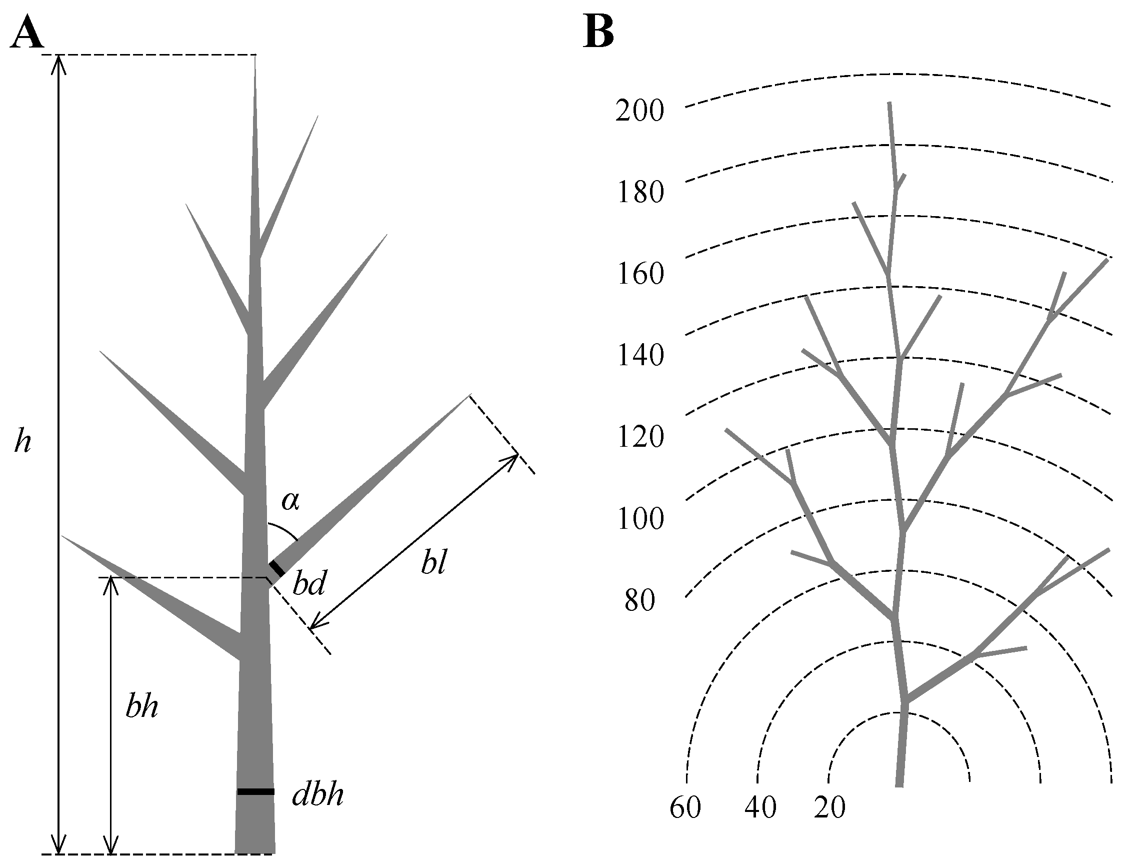
2.1. Destructive Biomass Measurements

We destructively measured 23 sample trees from a 38 year old beech stand which is part of the Forest Botanical Garden and Arboretum of the Faculty of Forest Sciences and Forest Ecology at Georg-August-Universität Göttingen (Lower Saxony, Germany: 51°33′20.2″N 9°57′46.7″E). The trees were not pruned, and branching patterns developed under natural conditions. The 23 sample trees used were subjectively selected so that they covered the dbh range of the stand, did not show any signs of crown damage, had developed single stems, and belonged to the dominant and co dominant layers. Suppressed trees were avoided in the selection process. One of the selection criteria was that the trees could be felled without causing damage to the branches. The study stand had on average 3984 trees·ha−1 larger than 5 cm in dbh, a dominant height of 15.9 m, a total basal area of 37.6 m2·ha−1 (37.0 m2·ha−1 of beech), and an average slope of 17% with south-east exposure. Other forest inventory characteristics of the study stand are presented in Table 1.
The sample trees were felled and measured in the winters of 2014/2015 (6 trees) and 2015/2016 (17 trees) in leaf-off state. All 23 sample trees were measured and destructively sampled to characterize the horizontal branch biomass distribution, while only the 17 trees in the second measuring survey (2015–16) were also scanned by TLS before cutting them into pieces. Summary statistics of the sample trees are in Table 1. The following measurements were made at each tree: the dbh of 23 all standing sample trees was measured to the nearest mm with a diameter tape; total height (h) and height of the first live branch were determined to the nearest dm with a clinometer; crown diameter (CD) was measured to the nearest cm with measuring tape and clinometer (to generate the zenithal directions); the crown ratio (CR) was calculated as the ratio between live crown length and h, where the lower end of the crown was defined by the insertion point in the stem of the first live branch. The trees were then carefully felled to avoid damaging the branches. For each first order branch (i.e., the branches originating from the stem) longer than 20 cm, the following variables were measured directly in the field: the distance from the stump height to the height of branching node (bh); the branch length (bl); the branch diameter (bd), measured perpendicularly to the branches´ axis at the closest possible position to the stem; and the vertical branch angle (α) (Figure 1A). The height of branching nodes bh and branch lengths bl were determined with a tape (mm resolution), branch diameter was measured with a precision caliper (0.01 mm resolution), and branch angle was determined with a digital goniometer (°). Measurement of the branch angle at the stem was necessary to estimate the horizontal position of the first order branches. In a simplified method, and to make measurements practicable, we assumed that first order branches were “flat” and extended from the stem to its end with all side-branches in a single plane (Figure 1B) defined by the vertical branch angle α, that is: the branch curvature or bending was not considered. An illustration of the measurements made in each sample tree is shown in Figure 1A. All first order branches shorter than 20 cm were assumed to have a value of α corresponding to the mean α of all first order branches longer than 20 cm.
For biomass measurements, all first order branches were cut and laid flat on a large plastic sheet on which concentric circles were drawn in steps of 20 cm radius so that the branch base (first order branching node) was located at the center of the circle (Figure 1B). Starting from the outer end, twigs and side-branches were cut consecutively into 20 cm circular rings defined by the outer radius of the ring. Fresh biomass was weighed in all branch elements within a circular ring with a digital scale, to the nearest gram. Composite samples of branches were then randomly collected for each 20 cm circular ring to predict wood dry matter after oven drying at 105 °C until constant weight. The biomass in each circular ring of each branch in the tree was then projected to the horizontal plane by using the branching angle α as measured before cutting the branch. By assuming that the horizontal distribution of crown biomass in radial direction is the same for all orientations in the horizontal plane (isotropic), we disregarded both a possible asymmetry of the crown projection shape and possible differences in biomass distribution over the horizontal angular range of 0 to 360° around the stem. The distribution of the total branch biomass for a given tree was obtained by projecting, branch by branch, the biomass observed at each circular ring.

2.2. Modelling the Individual Horizontal Woody Branch Biomass Distribution

The empirical biomass data resulting from the approach described in Section 2.1 allowed us to depict and model the individual tree branch biomass distribution as a function of the horizontal distance from the stem. The empirical branch biomass density and the crown radius were standardized and grouped into 20 classes of relative crown radii (rcr) for each tree. The observed horizontal branch biomass distribution for the 23 destructively sampled beech trees is shown in Figure 2, showing the same basic shape with some variability.
We fitted a horizontal biomass distribution model by the ordinary least squares (OLS) method with the rcr as the only predictor variable. The segmented polynomial model with a unique inflection point proposed by Max and Burkhardt [35] was used. This model has been developed and successfully applied to model stem taper curves and was selected due to its flexibility and because the pattern observed in Figure 2 is similar to the pattern observed in the relative diameter-relative height relationship of the stem taper curves (e.g. [36,37,38]). In Section 4 we argue about alternative model formulations that could be used to model the horizontal biomass distribution.
Goodness of fit was evaluated by means of the pseudo-coefficient of determination (R2*) and the root mean square error (RMSE), as previously described in Pérez-Cruzado et al. [39]. The formulation of the segmented polynomial model proposed by Max and Burkhardt [35] is as follows:
w = ( b 1 · ( r c r 1 ) + b 2 · ( r c r 2 1 ) + b 3 · ( a r c r ) 2 · m a x ( ( a r c r ) ,   0 ) ( a r c r ) ) 0.5 + ε ,
where w is the standardized branch biomass density at the relative crown radii rcr; a is the inflection point to be estimated; b1, b2, and b3 are the coefficients related to the polynomial terms to be estimated; and ε is a random error term.
As the data contain multiple observations (20 classes of relative radii) for each tree, autocorrelation within the residuals of each individual is expected, violating the assumption of independent error terms. An autoregressive error structure was therefore included in the model to account for autocorrelation. We used the Durbin–Watson test [40,41] to test for the presence of autocorrelation and evaluated the order of the autoregressive term by graphing the residuals against different lag residuals.
It is important to note that the horizontal branch biomass distribution has been standardized and, therefore, the model fitted does not immediately estimate absolute biomass values but its distribution only. For application to specific trees, the total branch biomass must therefore be predicted from other models, and the absolute biomass is then distributed along the standardized model identified.

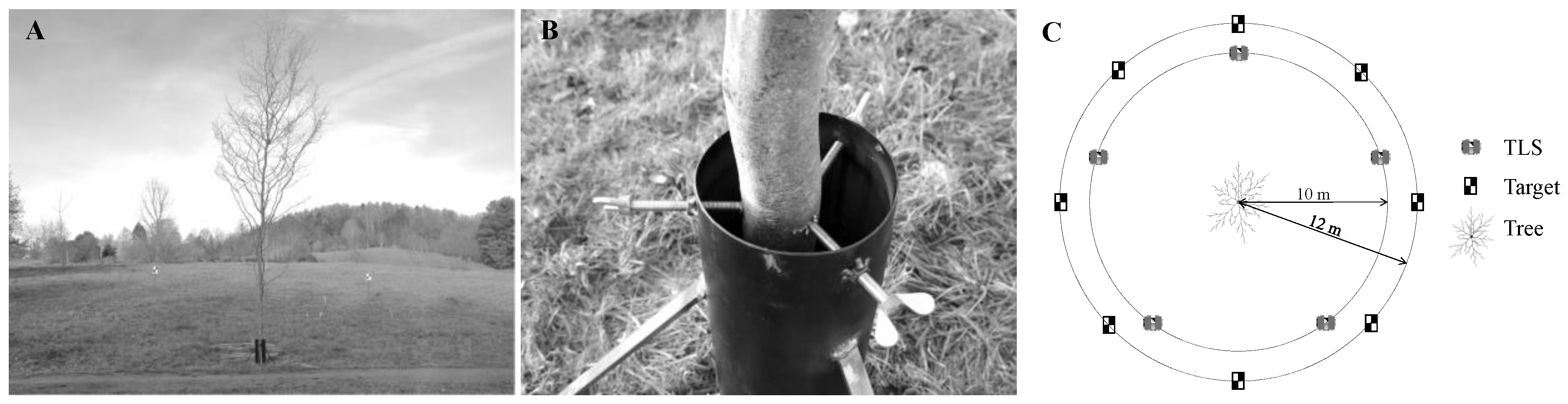
2.3. TLS Data Collection and Processing

We scanned a subset of 17 trees in the measuring campaign in 2015/2016 using the Trimble® TX5 3D laser scanner with a scan resolution of 177 Mpts per full scan, resulting in a scan duration of 3:35 min and a point spacing of approximately 3 mm at a distance of 10 m.
Analysis of terrestrial scans of individual trees in dense stands is extremely difficult because of overlapping crowns and the challenge of segmenting individual trees from the resulting point cloud. To avoid these challenges, after careful felling to avoid crown damages and before doing the destructive measurements described in Section 2.1, the trees were first brought to an open space where they were placed upright in a tailor-made tree holder (Figure 3A,B). Each tree was then scanned from five positions at constant horizontal distances of 10 m from the tree stem and distributed regularly (72°) around the tree (Figure 3C). The multi-scan TLS approach should reduce the occlusion problems that occur for complex objects like leaf-off tree crowns (as in our case) parts.
The five single scans were merged to a multi-scan single point cloud using the software Trimble Realworks®. For the target-based registration process, we used 8 artificial registration targets placed at a horizontal distance of 12 m from the tree holder and distributed regularly (45°) around the tree (Figure 3C). The maximum registration error was less than 5 mm.
The laser returns of the individual trees were manually extracted in the software CloudCompare® to remove returns from objects other than branches (Figure 4A). In a next step, the stems were manually deleted (Figure 4B). To remove noise, we used the CloudCompare’s “statistic outlier remover” SOR (PCL, 2011) (Figure 4C). Lastly, for graphical representation and modelling, the origin of the Cartesian grid system (x, y, z) was set to the stem position and the Z axis was aligned with the stem axis visually for each tree. For ellipsoidal-shaped crowns in the horizontal plane, the semi-minor and semi-major axes were aligned visually with the X and Y axes.

2.4. A New TLS Metric to Approximate Branch HBD

Empirical data collections, as described in Section 2.1, are extremely time consuming and expensive. For reference, the average time spent on destructive sampling per tree used in this study was four working days for two persons. To approximate the branch HBD, we developed a new TLS-based metric that we name Standardized Composite Histogram (SCH), which is generated from the crown laser returns. SCH is derived from the histogram of crown returns as a function of the horizontal distance to the stem axis, where, however, some adjustments were necessary:
  • The outer parts of the crown receive more hits than the inner parts.
  • After having removed the returns from the stem, as described in Section 2.3, the first order branches do not, of course, emerge directly from the one-dimensional stem axis but at a certain distance—the stem radius—which becomes smaller towards the top of the tree, as shown in Figure 4.
  • The outermost branches occlude the inner part of the crown.
  • The stem axis does not follow a perfect upright straight line and it has not been perfectly vertically erected on the stem center on the ground.
These four factors generate empty spaces with no returns in the position of the stem (see Figure 5), resulting in an undesired distribution of hits, which the computation of SCH is expected to solve.
To calculate the metric SCH, we projected the TLS returns to the horizontal plane and divided the point cloud in four quadrants as illustrated in Figure 5. This allowed to generate homogeneous groups regarding distance from the stem axis to the outermost crown projection, and reduces the effect of severe crown asymmetries in the horizontal plane. Separate histograms were produced for each quadrant and we later combined the four histograms into a single composite histogram. The objective of this procedure was reducing the effect of unbalances in occlusions among different parts of the crown. We assumed an ellipsoidal shape of the crown projection area, where the semi-major and semi-minor axis are aligned with the maximum and minimum distance among returns in the outermost point cloud projected in the horizontal plane as illustrated in Figure 5.
In the following, we describe step-by-step how to generate the Standardized Composite Histogram (SCH):
  • The horizontal distance to the stem axis (ρ) was calculated for each individual return by transforming the Cartesian coordinates of the original TLS point cloud to cylindrical coordinates (ρ, φ, z) with φ = azimuth and z = height:
    ρ = x 2 + y 2 ,
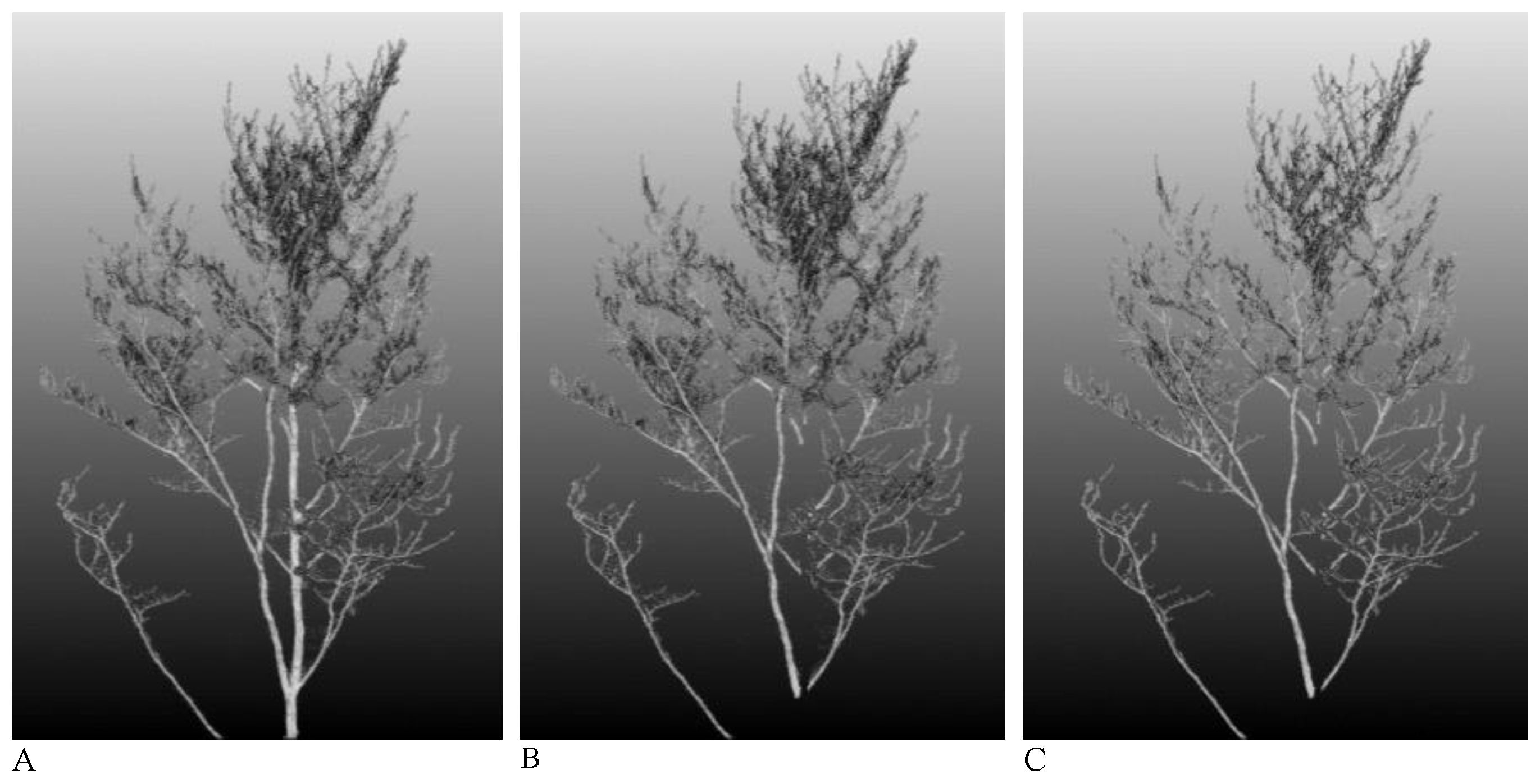
  • The crown returns were classified according to the four quadrants defined by the X and Y Cartesian coordinates in the horizontal plane (see Figure 5), and separate histograms were produced in each quadrant in 1 cm steps of ρ.
  • From steps one and two, the distribution of TLS returns can be determined for each quadrant. The starting point for each quadrant (ρSTART) was set to half of the range in ρ between 0 and the center of the bin with maximum observed frequency (Figure 6A,B). The entire histogram was then moved to the left by setting ρSTART as the starting point of the histogram (Figure 6C). The order for the k bins at the left of ρSTART was inverted, and the counts summed to the first k remaining bins (Figure 6D,E) so that the total number of hits captured in the distribution remained the same.
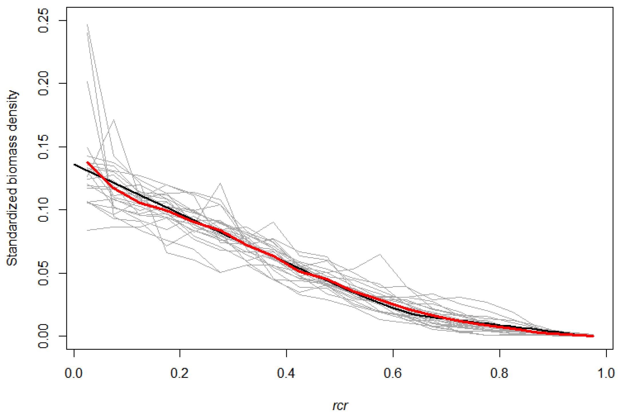
  • The resulting histograms for each quadrant (Figure 6E) were combined into a single histogram and then standardized in ρ relative to the maximum ρ across all quadrants. This is what we finally refer to as the standardized composite histogram (SCH).
  • The SCH was then grouped into new classes of relative ρ, and the counts were standardized with the total number of counts over all ρ classes.

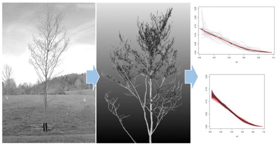
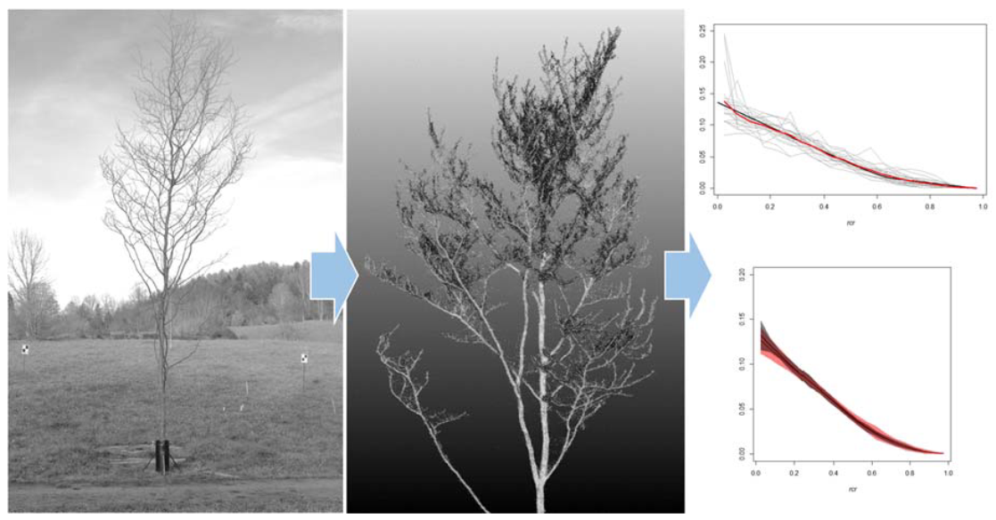
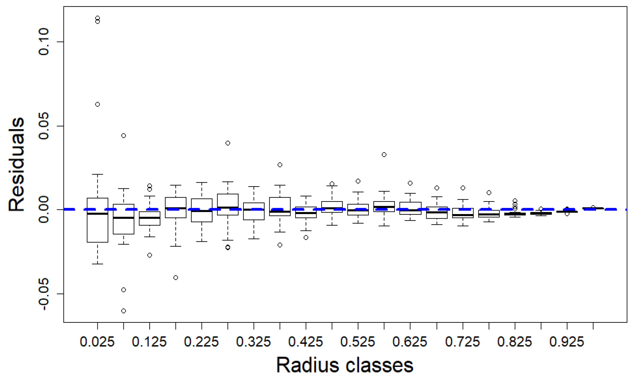
2.5. Evaluation of the TLS Metric SCH

To evaluate SCH to be used as a proxy for branch HBD, we first needed to adjust a model to the distribution of the TLS returns and then compare it to the empirical distribution from 2.1 which we use as a reference distribution. We fitted a non-parametric local polynomial regression (LOESS) model to both the empirical data from 2.1 and the TLS-based SCH metric, by using a smoothing parameter (α) of 0.75. The 95% confidence intervals were estimated for both the empirical data and the SCH metric: the overlap between these confidence intervals was used to assess their similarity and, therefore, the suitability of the SCH metric for use as a proxy for the branch HBD. The SCH metric was then calibrated to provide a better representation of the empirical data by computing the tree by tree differences between the raw SCH metric and the empirical data, and by then modelling these differences by LOESS. The possible need for this correction is raised because SCH is a metric of surface area, whereas HBD is about volume and biomass of (most likely) cylindrical shaped branches. We did not test tree-by-tree similarities in the empirical and SCH metric density functions as we were only interested in how the global empirical distribution was represented by the SCH metric. Statistical analyses and all computations were executed in R [42].

3. Results

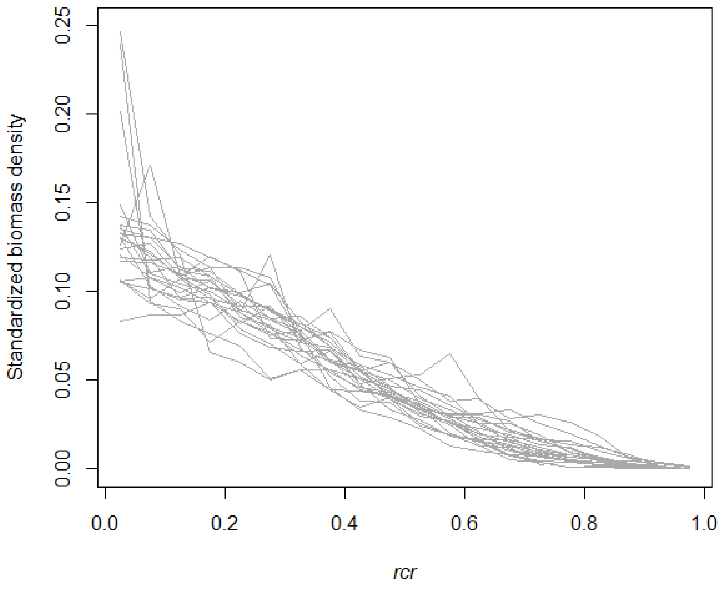
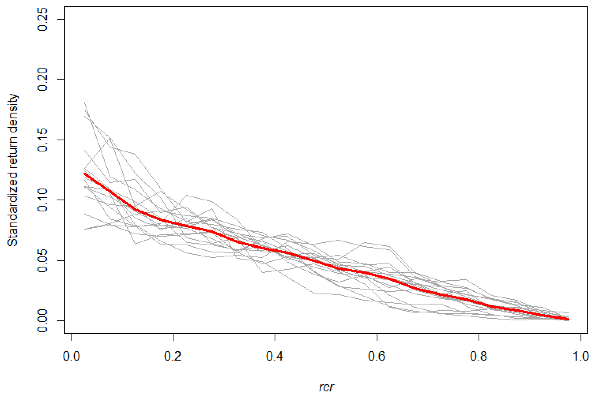
3.1. Empirical Branch HBD

The empirical horizontal branch biomass distribution estimated from the 23 destructively sampled trees is shown in Figure 7. As expected, the distribution follows an inverse J shape, with most of the branch biomass close to the stem. To some extent, the shape of these curves resembles that of the stem taper curves. The branch biomass is very variable, particularly closer to the stem—where the major portion of biomass occurs—and becomes smaller towards the crown edge where thinner branches dominate (Figure 7).
The segmented model proposed by Max and Burkhart [35] was initially fitted without expanding the error terms to account for autocorrelation. The Durbin–Watson test, however, indicated a significant positive serial correlation (d = 1.284). Graphs of residuals against lag residuals suggested the need to include a third-order autocorrelation term AR(3). After correcting for autocorrelation using the proposed error structure, the trends in residuals against lag residuals disappeared, and the Durbin–Watson test (d = 2.063) indicated the absence of significant correlation. The values of the goodness-of-fit statistics (R2* = 0.922 and RMSE = 0.00015) indicated a good fit, and all of the parameters simultaneously contributed to statistically significantly improving the quality of the fit of the model to the data (Table 2). Figure 7 (black line) illustrates the overall satisfactory fit.
To analyze the effect of each individual tree on the parameter estimates a, b1, b2, and b3 of Equation (1), we fitted the model independently for each of the 23 trees. The parameter estimates for b3 were very variable, with a coefficient of variation of 427.5%. Analysis of the correlation coefficients between the b3 parameter estimates and the main tree variables indicated a positive correlation with the crown ratio; we therefore generalized the base model (Equation (1)) by including a linear relationship of the parameter b3 with the crown ratio (CR) to finally obtain Equation (3) for the empirical branch biomass density distribution model:
w = ( b 1 · ( r c r 1 ) + b 2 · ( r c r 2 1 ) + ( b 31 + b 32 · C R ) · ( a r c r ) 2 · m a x ( ( a r c r ) ,   0 ) ( a r c r ) ) 0.5 + ε ,
where w is the standardized branch biomass density at the relative crown radii rcr; CR is the crown ratio; a is the inflection point to be estimated; b1, b2, b31 and b32 are the parameters related to the polynomial terms to be estimated; and ε is a random error term.
The generalized model explains 92.4% of the observed variability of the standardized branch biomass density (w) with a RMSE value of 0.000149, which is a 2.6% reduction relative to the original Equation (1). The value of the Durbin–Watson test was d = 2.062, indicating absence of significant autocorrelation after including the AR(3) structure in the model. All the parameters simultaneously contributed to statistically significantly improving the quality of the fit of the model to the data at a 5% level and the visual analysis of the residuals did not show any anomalous trend (Figure 8). The parameter estimates and the goodness of fit statistics are shown in Table 2.

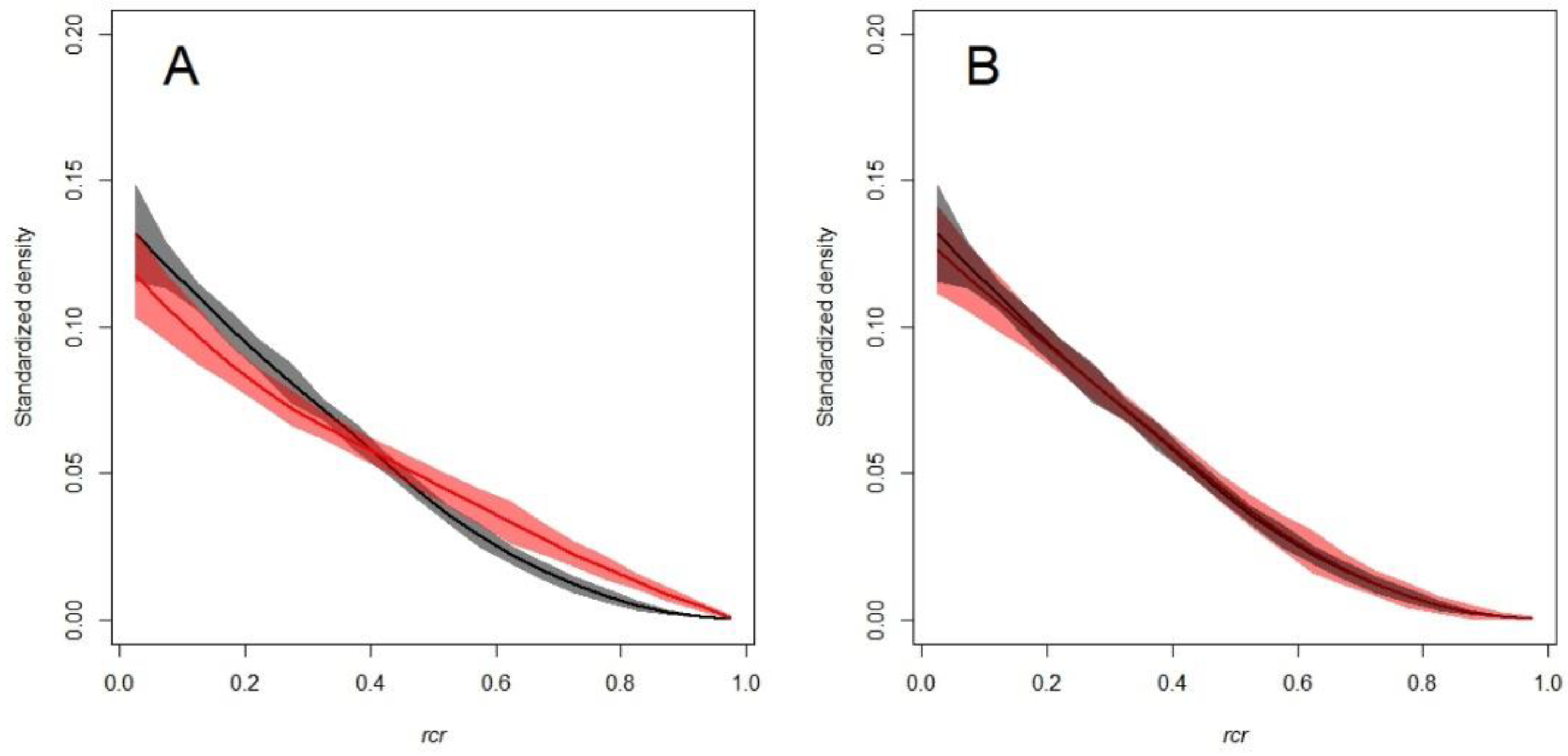
3.2. The SCH TLS Metric as a Proxy for the Branch HBD

Figure 9 illustrates the SCH metric built from the distribution of crown returns resulting from the TLS. The average number of returns per sample tree crown was 834,045 (SD = 390,296). The standardized return density obtained for the 17 scanned trees showed a similar horizontal branch biomass distribution to that obtained by destructive sampling (Figure 2 and Figure 7).
For a more objective analysis of this similarity, we generated the 95% confidence interval bands around the LOESS models for both the empirical data and the TLS-based metric SCH. The original data overlap with the raw values of the SCH metric (Figure 10A), although systematic deviations were found with the TLS-based model underestimating the biomass closer to the stem and overestimating the biomass towards the crown edge. This is probably due to the scanning geometry, which causes branches at the outer parts of the crowns to produce fewer scan occlusions than those closer to the stem. These differences were successfully corrected by modelling the differences with the empirical data by LOESS, as illustrated in Figure 10B.
Overall, the results indicate that the proposed SCH metric may be used as a proxy for the empirical branch biomass distribution, albeit adjustments were required.

4. Discussion

The individual tree horizontal biomass distribution is a basic element required to generate horizontal forest biomass distribution for application in forest inventory for biomass from fixed-area plots [7], and alike applications. It will also be of interest for remote sensing-based modelling of forest biomass when matching field plot biomass to remotely sensed data, as well as for many other ecological and forest management studies [7]. In the absence of available models as of yet, we chose two empirical pathways to construct our own models: (1) a destructive study of 23 trees and (2) combining the destructive sampling study with TLS which may help to increase sample size in a cost-efficient manner. All trees were beech trees of relatively small dimensions (dbh between 9.2 cm and 20.6 cm), with single stems and no irregularities. As both pathways yielded similar models whose shape resembles that of stem taper curves, we used well-known techniques to fit stem taper models. We observed correspondence between our TLS-based SCH metric and the empirical horizontal branch biomass distribution so that the presented TLS-based SCH metric bears potential for a rapid and straightforward approach to approximate the individual branch HBD, or to increase sample size in a cost-efficient manner. The similarity to taper curves was not surprising, as branch allometry has been reported to resemble stem allometry [43], because the crown horizontal biomass distribution is considered to be the sum of the biomass allocation in many branches constituting the crown (although with a multitude of geometrical arrangements), one may expect that the overall horizontal branch biomass distribution will have similar characteristics.
The fitting statistics of the model finally developed (OLS model) were similar to those obtained for taper curves [44,45,46,47,48,49,50], indicating the overall suitability of the model. The authors opted for the OLS model instead of others which are expected to yield improved goodness-of-fit statistics. This is the case for fitting subject (tree) specific models including random parameters by subject by using nonlinear mixed models (NME model). The main disadvantage for the NME model is the operational use, as the random parameters estimation for a new tree would require horizontal branch biomass density over relative crown radii (rcr) data, which is time-consuming to gather. When this information is not available, the NME model can still be used to estimate horizontal biomass from the fixed parameters of mixed-effects model, by assuming the random parameters are equal to zero (mean approach, M) or by computing mean predictions from the mixed-effects models over the distribution of random effects (population average approach PA). There is substantial evidence in the literature that prediction errors are greater for the M and PA approaches than for the OLS approach, and therefore, from the prediction point of view, the use of the mixed-effects models is not recommended when subject specific measurements are not available (e.g. [37,42,43,44,45,46,47]). Furthermore, although it is highly likely that there are random tree effects in the modelled relationship, it may lead to non-constant among-subject variances in the NME model. This is because tree effects are expected to be size-dependent, and then the NME model would be heteroskedastic caused in part by an error variance and a subject variance that may both depend on tree size (but not necessarily with identical dependency structures). Due to the above reasons, we opted for the OLS model.
The approach may be valuable for deriving the density function of the horizontal branch biomass distribution directly from basic geometric considerations of crown architecture, under the assumption that branching patterns are self-similar fractals. Our approach of directly adjusting the horizontal distribution of branch biomass is novel. It has the advantage over previous work that it does not require the use of voxel-based algorithms or 3D shape reconstruction [16,17,18,22,26,29,30,31]. Furthermore, this technique allows a good approximation of the biomass of small branches by TLS measurement, which has been found to be problematic in previous work [27,33]. This methodology ensures compatibility in individual tree-level estimates of total branch biomass with biomass equations. This is because the height of the distribution can easily be adjusted to ensure that the volume below it matches the branch biomass for a given tree, as described in Kleinn et al. [7]. Although our empirical approach of felling trees and re-erecting them in an open space for laser scanning and subsequent section-wise weighting of branch pieces enabled us to build first models from direct measurements (not only scans etc.), it is not operationally applicable to larger and irregular trees. However, in situ scans of selected trees by felling all surrounding trees may be an operational alternative for extending this study to non-easily handled tree dimensions. The results obtained in terms of correction of the SCH metric show that it is feasible to extend this study to other species or larger tree sizes by combining TLS scans and destructive analysis.
For our model of tree HBD we assumed (1) a circular crown projection area (2) around a perfectly upright stem which is easy to work with but not very realistic. However, any additional refinement of crown projection area assessment will have associated measurement cost. (3) The third assumption is isotropy: we assumed that in each vertical half plane laid through the stem axis the relative distribution of biomass will be the same. While some symmetry is logically required to guarantee physical stability of trees, perfect isotropy is a simplification. However, at this moment, we do not see how this assumption could operationally be replaced by a more realistic assessment in a field inventory context, unless laser scanning becomes much faster, cheaper and more accurate in terms of immediate reconstruction of tree crowns.

5. Conclusions

The following conclusions may be drawn from the study. First, the horizontal branch biomass distribution has been empirically described and modelled with model formulations known from taper curves; the fitting statistics of the resulting models were similar to those obtained for taper curves. Second, we derived a TLS-based metric named Standardized Composite Histogram (SCH) as a proxy of branch Horizontal Biomass Distribution (HBD); we observed correspondence between the SCH metric and the empirical HBD, indicating a possible way of increasing the efficiency in developing HBD models by combination of empirical measurements and TLS scans in some sample trees, and only TLS scans in a larger sample. Finally, considering the promising results obtained under the optimal scanning conditions of this study, further evaluation of the effect of factors such as taking TLS data with occlusions or reducing the number of scans on the performance of the proposed methodology would be relevant.
This first model of the horizontal distribution of crown biomass may support the improvement of precision of estimating biomass from field sampling (as recently illustrated in Kleinn et al. [7]). Further, we expect that remote-sensing-based models to predict biomass may benefit from the geometrically more specific determination of the plot biomass when applying the HBD to all sample trees within a fixed area plot.

Author Contributions

Conceptualization, C.K., L.F. and C.P.-C.; methodology, C.P.-C., L.F. and C.K.; software, N.N. and P.M.; formal analysis, C.P.-C. and J.G.Á.-G.; resources, C.K.; data curation, N.N., C.P.-C. and J.G.Á.-G.; writing—original draft preparation, C.P.-C.; writing—review and editing, C.P.-C., C.K., P.M., J.G.Á.-G., S.M., L.F. and N.N.; supervision, C.K.; project administration, C.K.; funding acquisition, C.K. All authors have read and agreed to the published version of the manuscript.

Funding

This research was funded by the Forest Research Institute of the German Federal State of Rheinland-Pfalz (FAWF) in Trippstadt. We also thank the Marie Sklodowska-Curie Action fellow QUAFORD and the Ramón y Cajal Tenure Track awarded to C.P.-C.

Informed Consent Statement

Not applicable.

Data Availability Statement

Not applicable.

Acknowledgments

We gratefully acknowledge the help received in fieldwork from a team of students from our international master programme TIF in Göttingen: many thanks to Najeeb Al-Amin Iddris, Huy Luan Hua, Lilian Huang Kuo, Parisa Mazinanian, and Didacus Tamambang. We thank Volker Meng from the Botanical Garden of the Forest Faculty in Göttingen for granting access and Torsten Vor, Silviculture and Forest Ecology of the Temperate Zones, for selecting and felling sample trees. Likewise, we thank three students from the Universidad de Oviedo, Spain, for supporting the laborious empirical study of determining branch biomass: Eatidal Amin Darei, Nelson Díaz Álvarez, and Carla Asunción Menéndez Coego. The Institute of Wood Biology and Wood Products at University of Göttingen allowed us to do the wood sample drying in their labs which is gratefully acknowledged.

Conflicts of Interest

The authors declare no conflict of interest.

References

  1. Ketterings, Q.M.; Coe, R.; van Noordwijk, M.; Ambagau, Y.; Palm, C.A. Reducing Uncertainty in the use of Allometric Biomass Equations for Predicting Above-Ground Tree Biomass in Mixed Secondary Forests. For. Ecol. Manag. 2001, 146, 199–209. [Google Scholar] [CrossRef]
  2. Pérez-Cruzado, C.; Rodríguez Soalleiro, R. Improvement in Accuracy of Aboveground Biomass Estimation in Eucalyptus Nitens Plantations: Effect of Bole Sampling Intensity and Explanatory Variables. For. Ecol. Manag. 2011, 261, 2016–2028. [Google Scholar] [CrossRef]
  3. Zianis, D.; Muukkonen, P.; Mäkipää, R.; Mencuccini, M. Biomass and Stem Volume Equations for Tree Species in Europe; Tammer-Paino Oy: Tampere, Finland, 2005; p. 63. [Google Scholar]
  4. Ruiz-González, A.D.; Álvarez-González, J.G. Canopy Bulk Density and Canopy Base Height Equations for Assessing Crown Fire Hazard in Pinus Radiata Plantations. Can. J. For. Res. 2011, 41, 839–850. [Google Scholar] [CrossRef]
  5. Jiménez, E.; Vega, J.A.; Ruiz-González, A.D.; Guijarro, M.; Alvarez-González, J.G.; Madrigal, J.; Cuiñas, P.; Hernando, C.; Fernández-Alonso, J.M. Carbon Emissions and Vertical Pattern of Canopy Fuel Consumption in Three Pinus pinaster Ait. Active Crown Fires in Galicia (NW Spain). Ecol. Eng. 2013, 54, 202–209. [Google Scholar] [CrossRef]
  6. Affleck, D.L.R.; Keyes, C.R.; Goodburn, J.M. Conifer Crown Fuel Modeling: Current Limits and Potential for Improvement. West. J. Appl. For. 2012, 27, 165–169. [Google Scholar] [CrossRef] [Green Version]
  7. Kleinn, C.; Magnussen, S.; Nölke, N.; Magdon, P.; Álvarez-González, J.G.; Fehrmann, L.; Pérez-Cruzado, C. Improving Precision of Field Inventory Estimation of Aboveground Biomass through an Alternative View on Plot Biomass. For. Ecosyst. 2020, 7, 1–10. [Google Scholar] [CrossRef]
  8. Næsset, E. Predicting Forest Stand Characteristics with Airborne Scanning Laser using a Practical Two-Stage Procedure and Field Data. Remote Sens. Environ. 2002, 80, 88–99. [Google Scholar] [CrossRef]
  9. Tahvanainen, T.; Forss, E. Individual Tree Models for the Crown Biomass Distribution of Scots Pine, Norway Spruce and Birch in Finland. For. Ecol. Manag. 2008, 255, 455–467. [Google Scholar] [CrossRef]
  10. Nemec, A.F.L.; Parish, R.; Goudie, J.W. Modelling Number, Vertical Distribution, and Size of Live Branches on Coniferous Tree Species in British Columbia. Can. J. For. Res. 2012, 42, 1072–1090. [Google Scholar] [CrossRef]
  11. Kershaw, J.A.; Maguire, D.A. Crown Structure in Western Hemlock, Douglas-Fir, and Grand Fir in Western Washington: Trends in Branch-Level Mass and Leaf Area. Can. J. For. Res. 1996, 25, 1897–1912. [Google Scholar] [CrossRef]
  12. Xu, M.; Harrington, T.B. Foliage Biomass Distribution of Loblolly Pine as Affected by Tree Dominance, Crown Size, and Stand Characteristics. Can. J. For. Res. 1998, 28, 887–892. [Google Scholar] [CrossRef]
  13. Mascaro, J.; Detto, M.; Asner, G.P.; Muller-Landau, H.C. Evaluating Uncertainty in Mapping Forest Carbon with Airborne LiDAR. Remote Sens. Environ. 2011, 115, 3770–3774. [Google Scholar] [CrossRef]
  14. Nielsen, C.C.N.; Mackenthum, G. Die horizontale Varia-tion der Feinwurzelintensität in Waldböden in Abhängigkeit vonder Bestockungsdichte. Einerechnerische Methode zur Bestimmung der “Wurzelintensitätsglocke” an Einzelbäumen. Allg. Forst. Jagdztg. 1991, 162, 112–119. [Google Scholar]
  15. Fehrmann, L.; Kuhr, M.; von Gadow, K. Zur Analyse Der Grobwurzelsysteme Großer Waldbäume and Fichte [Picea abies (L.) Karst.] Und Buche [Fagus sylvatica L.] (In German: “Analyis of the Coarse Root Systems of Large Trees at Spruce [Picea abies (L.) Karst.] and Beech [Fagus sylvatica L.]”). Forstarchiv 2003, 74, 96–102. [Google Scholar]
  16. Liang, X.; Kankare, V.; Hyyppä, J.; Wang, Y.; Kukko, A.; Haggrén, H.; Yu, X.; Kaartinen, H.; Jaakkola, A.; Guan, F. Terrestrial Laser Scanning in Forest Inventories. ISPRS J. Photogramm. Remote Sens. 2016, 115, 63–77. [Google Scholar] [CrossRef]
  17. Zhang, W.; Wan, P.; Wang, T.; Cai, S.; Chen, Y.; Jin, X.; Yan, G. A Novel Approach for the Detection of Standing Tree Stems from Plot-Level Terrestrial Laser Scanning Data. Remote Sens. 2019, 11, 211. [Google Scholar] [CrossRef] [Green Version]
  18. Pitkänen, T.P.; Raumonen, P.; Kangas, A. Measuring Stem Diameters with TLS in Boreal Forests by Complementary Fitting Procedure. ISPRS J. Photogramm. Remote Sens. 2019, 147, 294–306. [Google Scholar] [CrossRef]
  19. Zhu, Z.; Kleinn, C.; Nölke, N. Towards Tree Green Crown Volume: A Methodological Approach using Terrestrial Laser Scanning. Remote Sens. 2020, 12, 1841. [Google Scholar] [CrossRef]
  20. LaRue, E.A.; Wagner, F.W.; Fei, S.; Atkins, J.W.; Fahey, R.T.; Gough, C.M.; Hardiman, B.S. Compatibility of Aerial and Terrestrial LiDAR for Quantifying Forest Structural Diversity. Remote Sens. 2020, 12, 1407. [Google Scholar] [CrossRef]
  21. Guan, H.; Su, Y.; Sun, X.; Xu, G.; Li, W.; Ma, Q.; Wu, X.; Wu, J.; Liu, L.; Guo, Q. A Marker-Free Method for Registering Multi-Scan Terrestrial Laser Scanning Data in Forest Environments. ISPRS J. Photogramm. Remote Sens. 2020, 166, 82–94. [Google Scholar] [CrossRef]
  22. Calders, K.; Adams, J.; Armston, J.; Bartholomeus, H.; Bauwens, S.; Bentley, L.P.; Chave, J.; Danson, F.M.; Demol, M.; Disney, M.; et al. Terrestrial Laser Scanning in Forest Ecology: Expanding the Horizon. Remote Sens. Environ. 2020, 251, 112102. [Google Scholar] [CrossRef]
  23. Hauglin, M.; Astrup, R.; Gobakken, T.; Næsset, E. Estimating Single-Tree Branch Biomass of Norway Spruce with Terrestrial Laser Scanning using Voxel-Based and Crown Dimension Features. Scand. J. For. Res. 2013, 28, 456–469. [Google Scholar] [CrossRef]
  24. Cifuentes, R.; Van der Zande, D.; Farifteh, J.; Salas, C.; Coppin, P. Effects of Voxel Size and Sampling Setup on the Estimation of Forest Canopy Gap Fraction from Terrestrial Laser Scanning Data. Agric. For. Meteorol. 2014, 194, 230–240. [Google Scholar] [CrossRef]
  25. Grau, E.; Durrieu, S.; Fournier, R.; Gastellu-Etchegorry, J.P.; Yin, T. Estimation of 3D Vegetation Density with Terrestrial Laser Scanning Data using Voxels. A Sensitivity Analysis of Influencing Parameters. Remote Sens. Environ. 2017, 191, 373–388. [Google Scholar] [CrossRef]
  26. Hackenberg, J.; Spiecker, H.; Calders, K.; Disney, M.; Raumonen, P. SimpleTree—An Efficient Open Source Tool to Build Tree Models from TLS Clouds. Forests 2015, 6, 4245–4294. [Google Scholar] [CrossRef]
  27. Lau, A.; Bentley, L.P.; Martius, C.; Shenkin, A.; Bartholomeus, H.; Raumonen, P.; Malhi, Y.; Jackson, T.; Herold, M. Quantifying Branch Architecture of Tropical Trees using Terrestrial LiDAR and 3D Modelling. Trees 2018, 32, 1219–1231. [Google Scholar] [CrossRef] [Green Version]
  28. Park, H.; Lim, S.; Trinder, J.; Turner, R. 3D Surface Reconstruction of Terrestrial Laser Scanner Data for Forestry. In Proceedings of the 2010 IEEE International Geoscience and Remote Sensing Symposium, Honolulu, HI, USA, 25–30 July 2010; pp. 4366–4369. [Google Scholar]
  29. Raumonen, P.; Kaasalainen, M.; Åkerblom, M.; Kaasalainen, S.; Kaartinen, H.; Vastaranta, M.; Holopainen, M.; Disney, M.; Lewis, P. Fast Automatic Precision Tree Models from Terrestrial Laser Scanner Data. Remote Sens. 2013, 5, 491–520. [Google Scholar] [CrossRef] [Green Version]
  30. Disney, M.I.; Boni Vicari, M.; Burt, A.; Calders, K.; Lewis, S.L.; Raumonen, P.; Wilkes, P. Weighing Trees with Lasers: Advances, Challenges and Opportunities. Interface Focus 2018, 8, 20170048. [Google Scholar] [CrossRef] [PubMed] [Green Version]
  31. Calders, K.; Newnham, G.; Burt, A.; Murphy, S.; Raumonen, P.; Herold, M.; Culvenor, D.; Avitabile, V.; Disney, M.; Armston, J.; et al. Nondestructive Estimates of Above-ground Biomass using Terrestrial Laser Scanning. Methods Ecol. Evol. 2015, 6, 198–208. [Google Scholar] [CrossRef]
  32. Hackenberg, J.; Wassenberg, M.; Spiecker, H.; Sun, D. Non Destructive Method for Biomass Prediction Combining TLS Derived Tree Volume and Wood Density. Forests 2015, 6, 1274–1300. [Google Scholar] [CrossRef]
  33. Dassot, M.; Colin, A.; Santenoise, P.; Fournier, M.; Constant, T. Terrestrial Laser Scanning for Measuring the Solid Wood Volume, Including Branches, of Adult Standing Trees in the Forest Environment. Comput. Electron. Agric. 2012, 89, 86–93. [Google Scholar] [CrossRef]
  34. Abegg, M.; Kükenbrink, D.; Zell, J.; Schaepman, M.E.; Morsdorf, F. Terrestrial Laser Scanning for Forest Inventories—Tree Diameter Distribution and Scanner Location Impact on Occlusion. Forests 2017, 8, 184. [Google Scholar] [CrossRef] [Green Version]
  35. Max, T.A.; Burkhart, H.E. Segmented Polynomial Regression Applied to Taper Equations. For. Sci. 1976, 22, 283–289. [Google Scholar]
  36. Van Laar, A.; Akça, A. Forest Mensuration; Springer Science & Business Media: Berlin/Heidelberg, Germany, 2007. [Google Scholar]
  37. Burkhart, H.E.; Tomé, M. Modeling Forest Trees and Stands; Springer Science & Business Media: Dordercht, The Netherlands, 2012. [Google Scholar]
  38. Weiskittel, A.; Li, R. Development of Regional Taper and Volume Equations: Hardwood Species; Roth, B.E., Ed.; Cooperative Forestry Research Unit: 2011 Annual Report; University of Maine: Orono, ME, USA, 2012; pp. 76–84. [Google Scholar]
  39. Pérez-Cruzado, C.; Fehrmann, L.; Magdon, P.; Cañellas, I.; Sixto, H.; Kleinn, C. On the Site-Level Suitability of Biomass Models. Environ. Model. Softw. 2015, 73, 14–26. [Google Scholar] [CrossRef]
  40. Durbin, J.; Watson, G.S. Testing for Serial Correlation in Least Squares Regression: I. Biometrika 1950, 37, 409–428. [Google Scholar] [PubMed]
  41. Durbin, J.; Watson, G.S. Testing for Serial Correlation in Least Squares Regression. II. Biometrika 1951, 38, 159–177. [Google Scholar] [CrossRef] [PubMed]
  42. R Core Team. R: A Language and Environment for Statistical Computing; R Foundation for Statistical Computing: Vienna, Austria, 2018. [Google Scholar]
  43. Enquist, B.J. Universal Scaling in Tree and Vascular Plant Allometry: Toward a General Quantitative Theory Linking Plant Form and Function from Cells to Ecosystems. Tree Physiol. 2002, 22, 1045–1064. [Google Scholar] [CrossRef] [Green Version]
  44. Demaerschalk, J.P. Converting Volume Equations to Compatible Taper Equations. For. Sci. 1972, 18, 241–245. [Google Scholar] [CrossRef]
  45. Fang, Z.; Bailey, R.L. Compatible Volume and Taper Models with Coefficients for Tropical Species on Hainan Island in Southern China. For. Sci. 1999, 45, 85–100. [Google Scholar]
  46. Muhairwe, C.K. Taper Equations for Eucalyptus Pilularis and Eucalyptus Grandis for the North Coast in New South Wales, Australia. For. Ecol. Manag. 1999, 113, 251–269. [Google Scholar] [CrossRef]
  47. Fang, Z.; Borders, B.E.; Bailey, R.L. Compatible Volume-Taper Models for Lobolly and Slash Pine Based on a System with Segmented-Stem Form Factors. For. Sci. 2000, 46, 1–12. [Google Scholar]
  48. Castedo Dorado, F.; Dieguez-Aranda, U.; Barrio Anta, M.; Sánchez Rodríguez, M.; von Gadow, K. A Generalized Height-Diameter Model Including Random Components for Radiata Pine Plantations in Northwestern Spain. For. Ecol. Manag. 2006, 229, 202–213. [Google Scholar] [CrossRef]
  49. Westfall, J.A.; Scott, C.T. Taper Models for Commercial Tree Species in the Northeastern United States. For. Sci. 2010, 56, 515–528. [Google Scholar]
  50. Tang, X.; Pérez-Cruzado, C.; Fehrmann, L.; Álvarez-González, J.G.; Lu, Y.; Kleinn, C. Development of a Compatible Taper Function and Stand-Level Merchantable Volume Model for Chinese Fir Plantations. PLoS ONE 2016, 11, e0147610. [Google Scholar] [CrossRef] [PubMed] [Green Version]
Figure 1. Illustration of (A) the measurements made for each sample tree before felling, and (B) for individual branch measurements. dbh = diameter at breast height, h = tree height, bh = branch height at the stem, bd = branch base diameter, bl = branch length, and α = vertical branch angle.
Remotesensing 13 01041 g001
Figure 2. Observed horizontal branch biomass density over relative crown radii (rcr) for the 23 destructively sampled beech trees.
Remotesensing 13 01041 g002
Figure 3. A subset of 17 sample trees was carefully felled and re-erected (A) in an open space in (B) a tailor-made tree holder. These sample trees were then scanned (by TLS) using the scan and target locations as illustrated in (C).
Remotesensing 13 01041 g003
Figure 4. (A) Merged single tree point cloud. (B) Point cloud with stem axis removed. (C) after noise removal.
Remotesensing 13 01041 g004
Figure 5. Schematic representation of the branches in the crown, projected onto a horizontal plane, where we assumed an ellipsoidal shape of the crown projection with the semi-axes centered at the stem axis and thus defining four quadrants (I–IV). The returns in the surface of the stem were manually removed.
Remotesensing 13 01041 g005
Figure 6. Schematic representation of the computation of the standardized composite histogram (SCH) from the point cloud in the horizontal plane, conducted for each quadrant separately and subsequently combined (see text for explanation of histograms (AE)).
Remotesensing 13 01041 g006
Figure 7. Observed horizontal branch biomass distribution for the 23 destructively sampled beech trees (grey lines); the distribution of the average tree obtained using a non-parametric local regression (LOESS) with a smoothing span α = 0.75 (red line); and the fitted Max and Burkhart [35] segmented model (black line).
Remotesensing 13 01041 g007
Figure 8. Residual variability of horizontal branch biomass distribution per relative crown radius (rcr) class, where the dashed blue line corresponds to zero. The width of the radius classes is 0.05, and the midpoints are indicated by ticks on the x-axis. The same 20 classes of rcr have been considered as for Figure 2, Figure 7 and Figure 9.
Remotesensing 13 01041 g008
Figure 9. Standardized composite histogram (SCH) of the crown hits from TLS for the 17 scanned sample trees (grey lines). The red line represents the mean values obtained by LOESS.
Remotesensing 13 01041 g009
Figure 10. Comparison of the empirical horizontal branch biomass distribution (black) with (A) the original Standardized Composite Histogram obtained from Terrestrial Laser Scanning data (red) and (B) the Standardized Composite Histogram obtained by TLS data adjusted with the empirical data. The solid lines represent the mean local regression trends (smoothing span α = 0.75) and the shaded areas represent the 95% confidence intervals.
Remotesensing 13 01041 g010
Table 1. Statistics (1) of the stand from where the sample trees were taken (estimates, obtained from an inventory with n = 6), (2) of the trees for which the horizontal branch biomass distribution was measured after felling (n = 23) and (3) of the subset of 17 trees analyzed by terrestrial laser scanning (TLS) (dbh stands for diameter at breast height, h for total tree height and SD for standard deviation).
dbh (cm) h (m) Crown Ratio CRCrown Diameter CD (m)
RangeMeanSDRangeMeanSDRangeMeanSDRangeMeanSD
(1) Whole stand5.0–23.910.33.76.3–21.111.62.0------
(2) Empirical data9.2–20.614.03.013.3–21.117.72.20.437–0.8140.6120.0821.84–9.283.731.65
(3) TLS9.2–20.614.33.113.9–21.117.82.20.437–0.8140.6170.0871.84–9.283.851.82
Table 2. Parameter estimates for the horizontal branch biomass density distribution, where rho represents the estimated autocorrelation parameter.
Model (n = 460)ParameterEstimateStd. Error
Global model (Equation (1))b1−0.00470.0014
b20.00240.0007
b30.03660.0026
a0.66540.0208
rho0.35840.0436
Generalized model (Equation (2))b1−0.00530.0014
b20.00270.0007
b310.06790.0098
b32−0.04970.0142
a0.65410.0213
rho0.34290.0440
Publisher’s Note: MDPI stays neutral with regard to jurisdictional claims in published maps and institutional affiliations.

