
Fusion of GF and MODIS Data for Regional-Scale Grassland Community Classification with EVI2 Time-Series and Phenological Features

 ,
,  ,
,
Abstract
:
1. Introduction
2. Study Area and Data
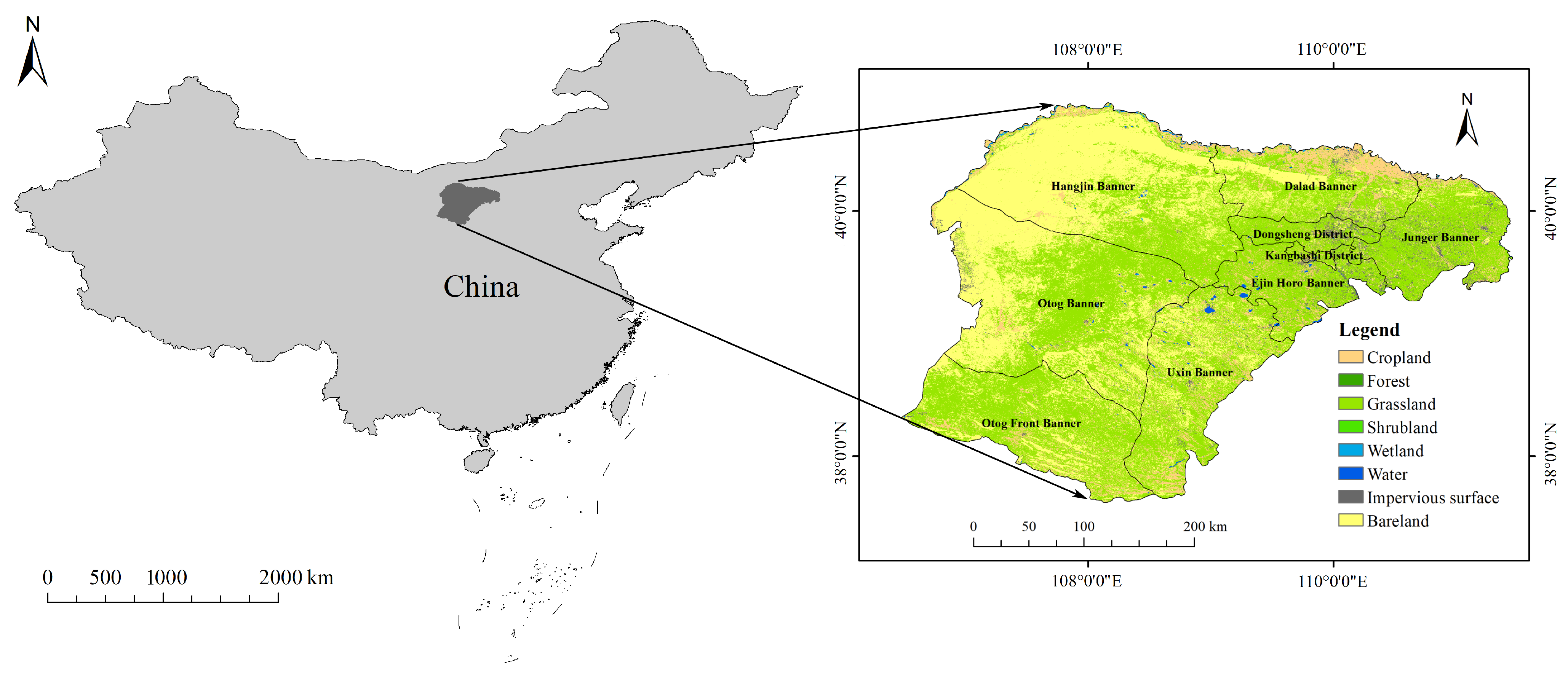
2.1. Study Area
2.2. GF-1, GF-6 Data and Pre-Processing
2.3. MODIS MOD09GA Dataset and Pre-Processing
2.4. Reference Data
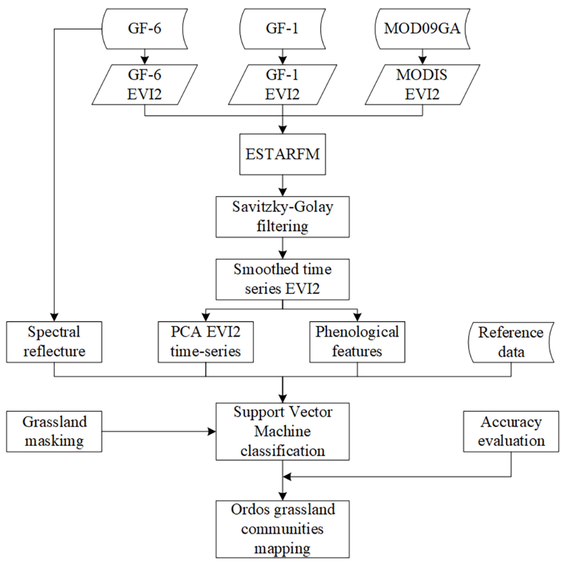
3. Methods
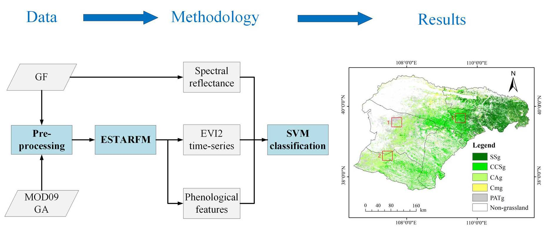
3.1. Generation of Cloudless EVI2 Time-Series by the Enhanced Spatial and Temporal Adaptive Reflectance Fusion Model (ESTARFM) Algorithm
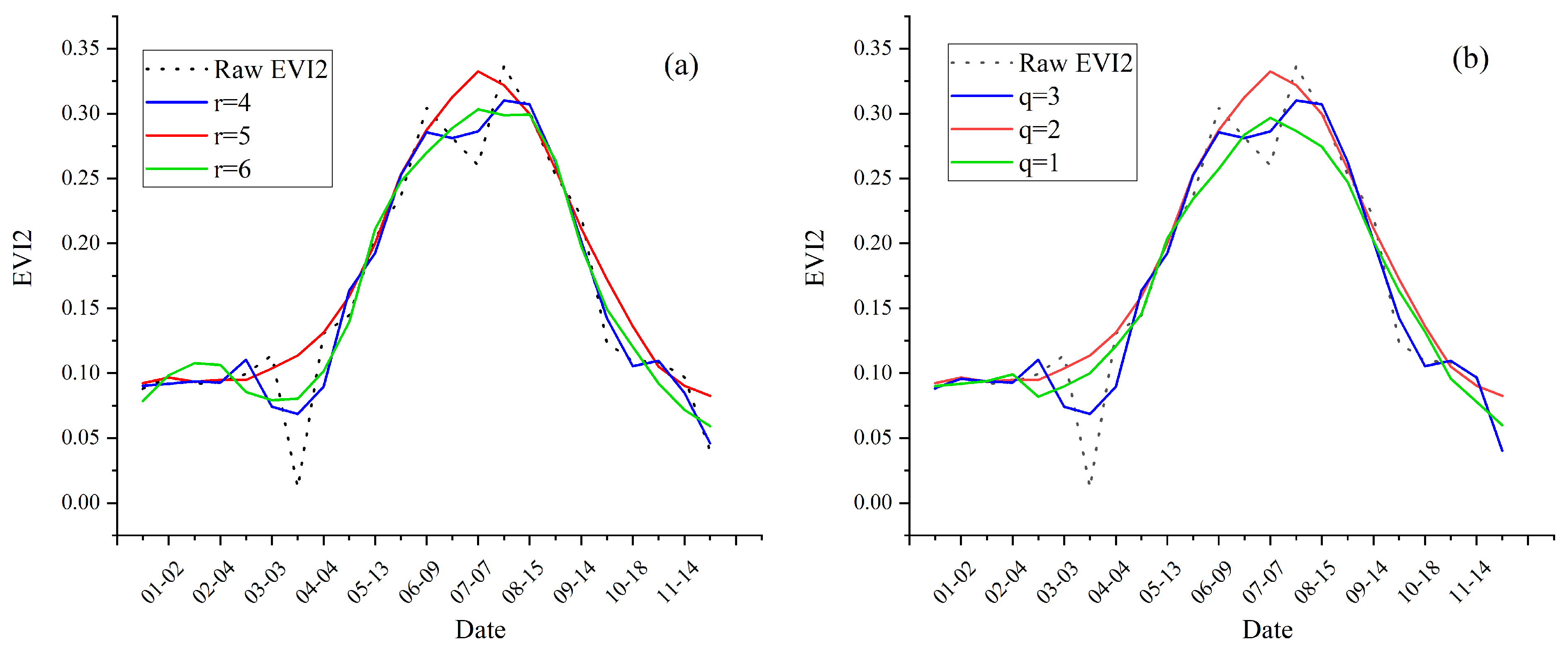
3.2. Reconstruction of Smoothed EVI2 Time-Series
3.3. Extraction of Phenological Features and PCA EVI2 Time-Series
3.4. SVM Classification and Accuracy Assessment
4. Results
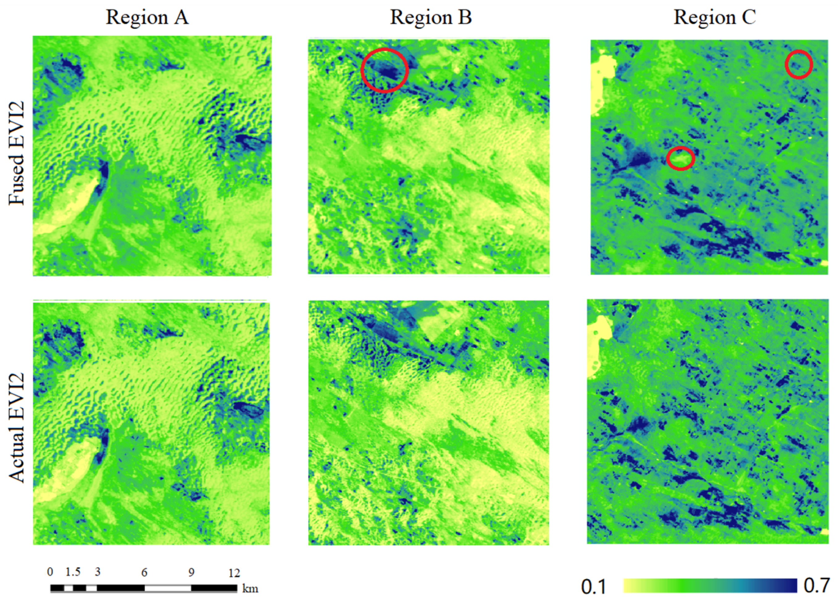
4.1. Accuracy Assessment of the ESTARFM Fusion
4.2. Pheonological Information Analysis
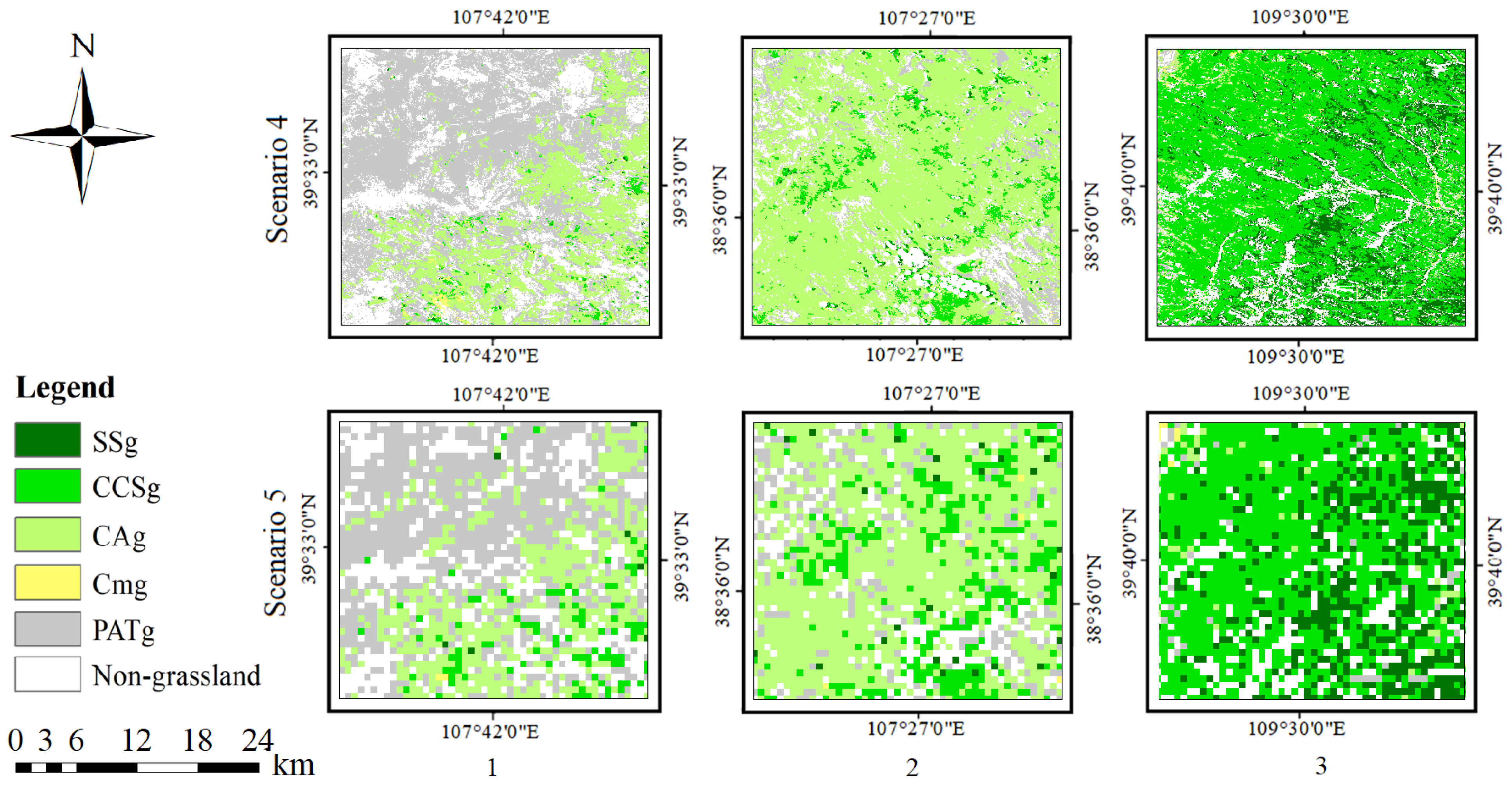
4.3. Accuracy Evaluation of Different Scenarios
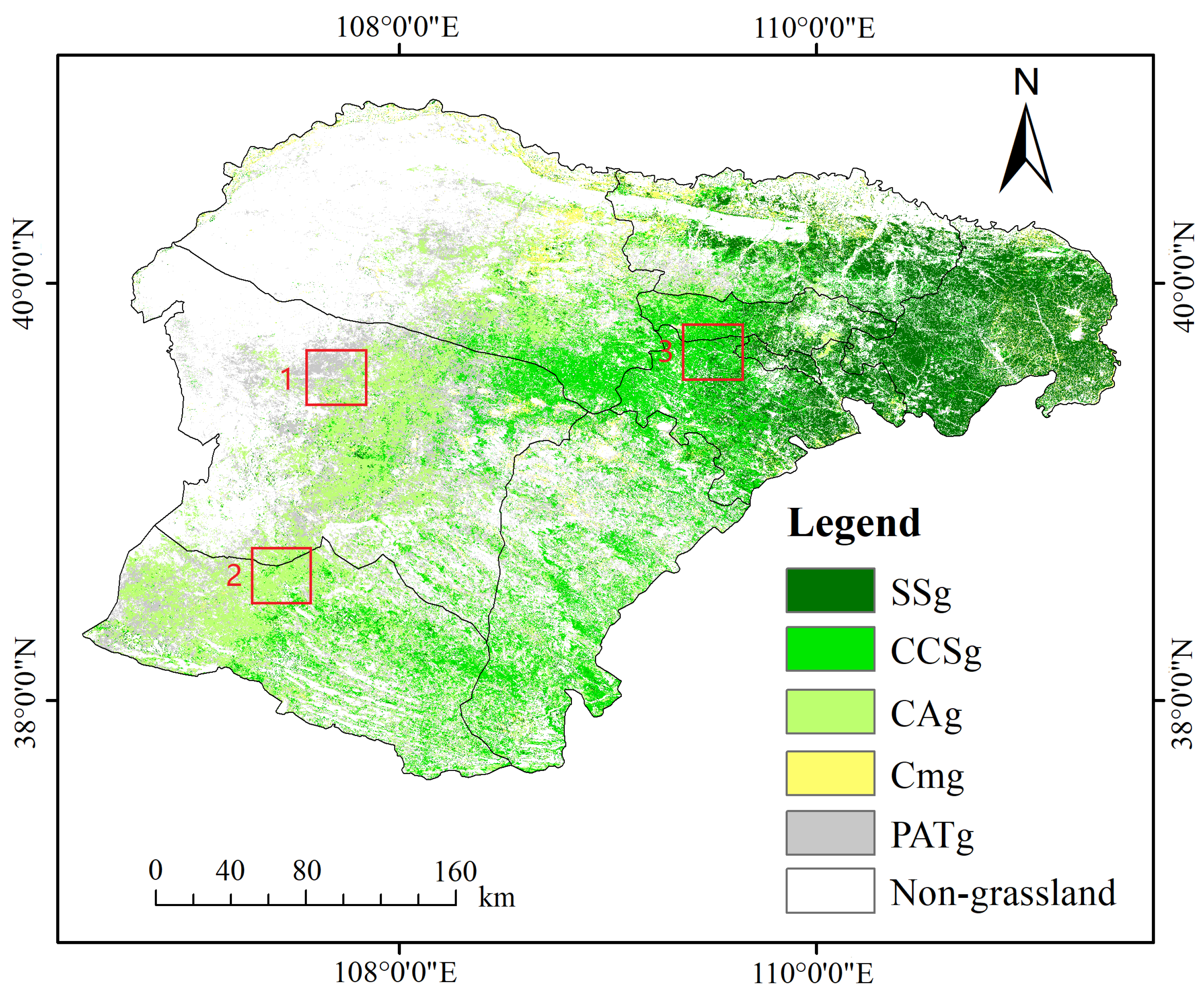
4.4. Grassland Communities Mapping in Ordos at 16 m Resolution
5. Discussion
5.1. Applicability of GF-1/6 Satellite Data in Regional-Scale Grassland Communities Classification
5.2. Limitation of ESTARFM Algorithm
5.3. Grassland Classification in Ordos
6. Conclusions
Author Contributions
Funding
Data Availability Statement
Acknowledgments
Conflicts of Interest
References
- Zillmann, E.; Gonzalez, A.; Herrero, E.J.M.; van Wolvelaer, J.; Esch, T.; Keil, M.; Weichelt, H.; Garzón, A.M. Pan-European grassland mapping using seasonal statistics from multisensor image time series. IEEE J. Sel. Top. Appl. Earth Obs. Remote Sens. 2014, 7, 3461–3472. [Google Scholar] [CrossRef]
- Xu, D. Distribution Change and Analysis of Different Grassland Types in Hulunber Grassland. Ph.D. Thesis, Chinese Academy of Agricultural Sciences Dissertation, Beijing, China, 2019. [Google Scholar]
- Lu, B.; He, Y. Species classification using Unmanned Aerial Vehicle (UAV)-acquired high spatial resolution imagery in a heterogeneous grassland. ISPRS J. Photogramm. Remote Sens. 2017, 128, 73–85. [Google Scholar] [CrossRef]
- Price, K.P.; Guo, X.; Stiles, J.M. Comparison of Landsat TM and ERS-2 SAR data for discriminating among grassland types and treatments in eastern Kansas. Comput. Electron. Agric. 2002, 37, 157–171. [Google Scholar] [CrossRef]
- Raab, C.; Stroh, H.G.; Tonn, B.; Meißner, M.; Rohwer, N.; Balkenhol, N.; Isselstein, J. Mapping semi-natural grassland communities using multi-temporal RapidEye remote sensing data. Int. J. Remote Sens. 2018, 39, 5638–5659. [Google Scholar] [CrossRef]
- Cui, X.; Guo, Z.G.; Liang, T.G.; Shen, Y.Y.; Liu, X.Y.; Liu, Y. Classification management for grassland using MODIS data: A case study in the Gannan region, China. Int. J. Remote Sens. 2012, 33, 3156–3175. [Google Scholar] [CrossRef]
- Yao, F.; Tang, Y.; Wang, P.; Zhang, J. Estimation of maize yield by using a process-based model and remote sensing data in the Northeast China Plain. Phys. Chem. Earth 2015, 87, 142–152. [Google Scholar] [CrossRef]
- Zlinszky, A.; Schroiff, A.; Kania, A.; Deák, B.; Mücke, W.; Vári, Á.; Székely, B.; Pfeifer, N. Categorizing grassland vegetation with full-waveform airborne laser scanning: A feasibility study for detecting Natura 2000 habitat types. Remote Sens. 2014, 6, 8056–8087. [Google Scholar] [CrossRef] [Green Version]
- Marcinkowska-Ochtyra, A.; Jarocińska, A.; Bzdęga, K.; Tokarska-Guzik, B. Classification of expansive grassland species in different growth stages based on hyperspectral and LiDAR data. Remote Sens. 2018, 10, 2019. [Google Scholar] [CrossRef] [Green Version]
- Melville, B.; Lucieer, A.; Aryal, J. Classification of lowland native grassland communities using hyperspectral Unmanned Aircraft System (UAS) Imagery in the Tasmanian midlands. Drones 2019, 3, 5. [Google Scholar] [CrossRef] [Green Version]
- Lu, B.; He, Y. Optimal spatial resolution of Unmanned Aerial Vehicle (UAV)-acquired imagery for species classification in a heterogeneous grassland ecosystem. GISci. Remote Sens. 2018, 55, 205–220. [Google Scholar] [CrossRef]
- Jarocińska, A.; Kopeć, D.; Tokarska-Guzik, B.; Raczko, E. Intra-Annual Variabilities of Rubus caesius L. Discrimination on Hyperspectral and LiDAR Data. Remote Sens. 2021, 13, 107. [Google Scholar] [CrossRef]
- Clark, M.L. Comparison of simulated hyperspectral HyspIRI and multispectral Landsat 8 and Sentinel-2 imagery for multi-seasonal, regional land-cover mapping. Remote Sens. Environ. 2017, 200, 311–325. [Google Scholar] [CrossRef]
- Hościło, A.; Lewandowska, A. Mapping forest type and tree species on a regional scale using multi-temporal Sentinel-2 data. Remote Sens. 2019, 11, 929. [Google Scholar] [CrossRef] [Green Version]
- Ochtyra, A.; Marcinkowska-Ochtyra, A.; Raczko, E. Threshold-and trend-based vegetation change monitoring algorithm based on the inter-annual multi-temporal normalized difference moisture index series: A case study of the Tatra Mountains. Remote Sens. Environ. 2020, 249, 112026. [Google Scholar] [CrossRef]
- Hong, G.; Zhang, A.; Zhou, F.; Brisco, B. Integration of optical and synthetic aperture radar (SAR) images to differentiate grassland and alfalfa in Prairie area. Int. J. Appl. Earth Obs. Geoinf. 2014, 28, 12–19. [Google Scholar] [CrossRef]
- Ouyang, W.; Hao, F.; Skidmore, A.K.; Groen, T.A.; Toxopeus, A.G.; Wang, T. Integration of multi-sensor data to assess grassland dynamics in a Yellow River sub-watershed. Ecol. India. 2012, 18, 163–170. [Google Scholar] [CrossRef]
- Hill, M.J. Vegetation index suites as indicators of vegetation state in grassland and savanna: An analysis with simulated SENTINEL 2 data for a North American transect. Remote Sens. Environ. 2013, 137, 94–111. [Google Scholar] [CrossRef]
- Yang, L.; Jin, S.; Danielson, P.; Homer, C.; Gass, L.; Bender, S.M.; Casei, A.; Costellog, C.; Dewitzd, J.; Fryc, J.; et al. A new generation of the United States National Land Cover Database: Requirements, research priorities, design, and implementation strategies. ISPRS J. Photogramm. Remote Sens. 2018, 146, 108–123. [Google Scholar] [CrossRef]
- McInnes, W.S.; Smith, B.; McDermid, G.J. Discriminating native and nonnative grasses in the dry mixedgrass prairie with MODIS NDVI time series. IEEE J. Sel. Top. Appl. Earth Obs. Remote Sens. 2015, 8, 1395–1403. [Google Scholar] [CrossRef]
- Rapinel, S.; Mony, C.; Lecoq, L.; Clement, B.; Thomas, A.; Hubert-Moy, L. Evaluation of Sentinel-2 time-series for mapping floodplain grassland plant communities. Remote Sens. Environ. 2019, 223, 115–129. [Google Scholar] [CrossRef]
- Wen, Q.; Zhang, Z.; Liu, S.; Wang, X.; Wang, C. Classification of grassland types by MODIS time-series images in Tibet, China. IEEE J. Sel. Top. Appl. Earth Obs. Remote Sens. 2010, 3, 404–409. [Google Scholar] [CrossRef]
- Schuster, C.; Schmidt, T.; Conrad, C.; Kleinschmit, B.; Förster, M. Grassland habitat mapping by intra-annual time series analysis—Comparison of RapidEye and TerraSAR-X satellite data. Int. J. Appl. Earth Obs. Geoinf. 2015, 34, 25–34. [Google Scholar] [CrossRef]
- Franke, J.; Keuck, V.; Siegert, F. Assessment of grassland use intensity by remote sensing to support conservation schemes. J. Nat. Conserv. 2012, 20, 125–134. [Google Scholar] [CrossRef]
- Shi-Bo, F.; Xin-Shi, Z. Control of vegetation distribution: Climate, geological substrate, and geomorphic factors. A case study of grassland in Ordos, Inner Mongolia, China. Can. J. Remote Sens. 2013, 39, 167–174. [Google Scholar] [CrossRef]
- Schmidt, T.; Schuster, C.; Kleinschmit, B.; Förster, M. Evaluating an intra-annual time series for grassland classification—How many acquisitions and what seasonal origin are optimal? IEEE J. Sel. Top. Appl. Earth Obs. Remote Sens. 2014, 7, 3428–3439. [Google Scholar] [CrossRef]
- Park, D.S.; Breckheimer, I.; Williams, A.C.; Law, E.; Ellison, A.M.; Davis, C.C. Herbarium specimens reveal substantial and unexpected variation in phenological sensitivity across the eastern United States. Phil. Trans. R. Soc. B 2019, 374, 20170394. [Google Scholar] [CrossRef] [PubMed]
- Wang, C.; Long, R.; Ding, L. The effects of differences in functional group diversity and composition on plant community productivity in four types of alpine meadow communities. Biodivers. Sci. 2004, 12, 403–409. [Google Scholar]
- Wang, C.; Guo, H.; Zhang, L.; Qiu, Y.; Sun, Z.; Liao, J.; Liu, G.; Zhang, Y. Improved alpine grassland mapping in the Tibetan Plateau with MODIS time series: A phenology perspective. Int. J. Digit. Earth 2015, 8, 133–152. [Google Scholar] [CrossRef]
- Yoo, C.; Im, J.; Park, S.; Quackenbush, L.J. Estimation of daily maximum and minimum air temperatures in urban landscapes using MODIS time series satellite data. ISPRS J. Photogramm. Remote Sens. 2018, 137, 149–162. [Google Scholar] [CrossRef]
- Zhou, J.; Jia, L.; Menenti, M. Reconstruction of global MODIS NDVI time series: Performance of Harmonic ANalysis of Time Series (HANTS). Remote Sens. Environ. 2015, 163, 217–228. [Google Scholar] [CrossRef]
- Yang, X.; Yang, T.; Ji, Q.; He, Y.; Ghebrezgabher, M.G. Regional-scale grassland classification using moderate-resolution imaging spectrometer datasets based on multistep unsupervised classification and indices suitability analysis. J. Appl. Remote Sens. 2014, 8, 083548. [Google Scholar] [CrossRef]
- Xu, K.; Tian, Q.; Yang, Y.; Yue, J.; Tang, S. How up-scaling of remote-sensing images affects land-cover classification by comparison with multiscale satellite images. J. Appl. Remote Sens. 2019, 40, 2784–2810. [Google Scholar] [CrossRef]
- Zheng, L. Crop Classification Using Multi-Features of Chinese Gaofen-1/6 Sateliite Remote Sensing Images. Ph.D. Thesis, University of Chinese Academy of Sciences, Beijing, China, 2019. [Google Scholar]
- Kong, F.; Li, X.; Wang, H.; Xie, D.; Li, X.; Bai, Y. Land cover classification based on fused data from GF-1 and MODIS NDVI time series. Remote Sens. 2016, 8, 741. [Google Scholar] [CrossRef] [Green Version]
- Jin, S.; Homer, C.; Yang, L.; Xian, G.; Fry, J.; Danielson, P.; Townsend, P.A. Automated cloud and shadow detection and filling using two-date Landsat imagery in the USA. Int. J. Remote Sens. 2013, 34, 1540–1560. [Google Scholar] [CrossRef]
- Zhang, H.K.; Huang, B. A new look at image fusion methods from a Bayesian perspective. Remote Sens. 2015, 7, 6828–6861. [Google Scholar] [CrossRef] [Green Version]
- Tao, G.; Jia, K.; Zhao, X.; Wei, X.; Xie, X.; Zhang, X.; Wang, B.; Yao, Y.; Zhang, X. Generating High Spatio-Temporal Resolution Fractional Vegetation Cover by Fusing GF-1 WFV and MODIS Data. Remote Sens. 2019, 11, 2324. [Google Scholar] [CrossRef] [Green Version]
- Yang, G.; Weng, Q.; Pu, R.; Gao, F.; Sun, C.; Li, H.; Zhao, C. Evaluation of ASTER-like daily land surface temperature by fusing ASTER and MODIS data during the HiWATER-MUSOEXE. Remote Sens. 2016, 8, 75. [Google Scholar] [CrossRef] [Green Version]
- Tewes, A.; Thonfeld, F.; Schmidt, M.; Oomen, R.J.; Zhu, X.; Dubovyk, O.; Menz, G.; Schellberg, J. Using RapidEye and MODIS data fusion to monitor vegetation dynamics in semi-arid rangelands in South Africa. Remote Sens. 2015, 7, 6510–6534. [Google Scholar] [CrossRef] [Green Version]
- Zhou, X.; Wang, P.; Tansey, K.; Zhang, S.; Li, H.; Wang, L. Developing a fused vegetation temperature condition index for drought monitoring at field scales using Sentinel-2 and MODIS imagery. Comput. Electron. Agric. 2020, 168, 105144. [Google Scholar] [CrossRef]
- Wu, M.; Huang, W.; Niu, Z.; Wang, C. Combining HJ CCD, GF-1 WFV and MODIS data to generate daily high spatial resolution synthetic data for environmental process monitoring. Int. J. Environ. Res. Public Health 2015, 12, 9920–9937. [Google Scholar] [CrossRef] [PubMed] [Green Version]
- Gao, F.; Masek, J.; Schwaller, M.; Hall, F. On the blending of the Landsat and MODIS surface reflectance: Predicting daily Landsat surface reflectance. IEEE Trans. Geosci. Remote Sens. 2006, 44, 2207–2218. [Google Scholar]
- Zhu, X.; Chen, J.; Gao, F.; Chen, X.; Masek, J.G. An enhanced spatial and temporal adaptive reflectance fusion model for complex heterogeneous regions. Remote Sens. Environ. 2010, 114, 2610–2623. [Google Scholar] [CrossRef]
- Zhang, H. Evalution on Sustainable Development of Animal Husbandry in Erdos City. Master’s Thesis, Inner Mongolia University, Hohhot, China, 2010. [Google Scholar]
- Jiang, Z.; Huete, A.R.; Didan, K.; Miura, T. Development of a two-band enhanced vegetation index without a blue band. Remote Sens. Environ. 2008, 112, 3833–3845. [Google Scholar] [CrossRef]
- Gong, P.; Liu, H.; Zhang, M.; Li, C.; Wang, J.; Huang, H.; Clinton, N.; Ji, L.; Li, W.; Bai, Y.; et al. Stable classification with limited sample: Transferring a 30-m resolution sample set collected in 2015 to mapping 10-m resolution global land cover in 2017. Sci. Bull. 2019, 64, 370–373. [Google Scholar] [CrossRef] [Green Version]
- Liu, G. Inner Mongolia Region. In Atlas of Physical Geography of China; China Map Press: Beijing, China, 2010; pp. 171–172. [Google Scholar]
- Zhang, X. Scrub, Desert, and Steppe. In Vegetation and Its Geographical Pattern in China: An Illustration of the Vegetation Map of the People’s Republic of China (1:1000000); Geological Publishing House: Beijing, China, 2007; pp. 257–385. [Google Scholar]
- Jia, K.; Liang, S.; Gu, X.; Baret, F.; Wei, X.; Wang, X.; Yao, Y.; Yang, L.; Li, Y. Fractional vegetation cover estimation algorithm for Chinese GF-1 wide field view data. Remote Sens. Environ. 2016, 177, 184–191. [Google Scholar] [CrossRef]
- Yang, A.; Zhong, B.; Hu, L.; Wu, S.; Xu, Z.; Wu, H.; Wu, J.; Gong, X.; Wang, H.; Liu, Q. Radiometric Cross-Calibration of the Wide Field View Camera Onboard GaoFen-6 in Multispectral Bands. Remote Sens. 2020, 12, 1037. [Google Scholar] [CrossRef] [Green Version]
- Dobreva, I.D.; Klein, A.G. Fractional snow cover mapping through artificial neural network analysis of MODIS surface reflectance. Remote Sens. Environ. 2012, 115, 3355–3366. [Google Scholar] [CrossRef] [Green Version]
- Xun, L.; Zhang, J.; Cao, D.; Zhang, S.; Yao, F. Crop Area Identification Based on Time Series EVI2 and Sparse Representation Approach: A Case Study in Shandong Province, China. IEEE Access 2019, 7, 157513–157523. [Google Scholar] [CrossRef]
- Savitzky, A.; Golay, M.J. Smoothing and differentiation of data by simplified least squares procedures. Anal. Chem. 1964, 36, 1627–1639. [Google Scholar] [CrossRef]
- Chen, J.; Jönsson, P.; Tamura, M.; Gu, Z.; Matsushita, B.; Eklundh, L. A simple method for reconstructing a high-quality NDVI time-series data set based on the Savitzky–Golay filter. Remote Sens. Environ. 2004, 91, 332–344. [Google Scholar] [CrossRef]
- Reed, B.C.; Schwartz, M.D.; Xiao, X. Remote sensing phenology. In Phenology of Ecosystem Processes; Noormets, A., Ed.; Springer: New York, NY, USA, 2009; pp. 231–246. [Google Scholar]
- Ren, J.; Zabalza, J.; Marshall, S.; Zheng, J. Effective feature extraction and data reduction in remote sensing using hyperspectral imaging [applications corner]. IEEE Signal Process. Mag. 2014, 31, 149–154. [Google Scholar] [CrossRef] [Green Version]
- Zhong, L.; Hu, L.; Zhou, H. Deep learning based multi-temporal crop classification. Remote Sens. Environ. 2019, 221, 430–443. [Google Scholar] [CrossRef]
- Kabir, S.; Islam, R.U.; Hossain, M.S.; Andersson, K. An integrated approach of belief rule base and deep learning to predict air pollution. Sensors 2020, 20, 1956. [Google Scholar] [CrossRef] [PubMed] [Green Version]
- Su, P.; Li, G.; Wu, C.; Vijay-Shanker, K. Using distant supervision to augment manually annotated data for relation extraction. PLoS ONE 2019, 14, e0216913. [Google Scholar] [CrossRef] [PubMed] [Green Version]
- Xiong, Z.; Yu, Q.; Sun, T.; Chen, W.; Wu, Y.; Yin, J. Super-resolution reconstruction of real infrared images acquired with unmanned aerial vehicle. PLoS ONE 2020, 15, e0234775. [Google Scholar] [CrossRef]
- Lopatin, J.; Fassnacht, F.E.; Kattenborn, T.; Schmidtlein, S. Mapping plant species in mixed grassland communities using close range imaging spectroscopy. Remote Sens. Environ. 2017, 201, 12–23. [Google Scholar] [CrossRef]
- Tan, C.; Zhang, P.; Zhang, Y.; Zhou, X.; Wang, Z.; Du, Y.; Mao, W.; Li, W.; Wang, D.; Guo, W. Rapid Recognition of Field-Grown Wheat Spikes Based on a Superpixel Segmentation Algorithm Using Digital Images. Front. Plant Sci. 2020, 11, 259. [Google Scholar] [CrossRef] [Green Version]
- Maulik, U.; Chakraborty, D. Remote sensing image classification: A survey of support-vector-machine-based advanced techniques. IEEE Geosci. Remote Sens. Mag. 2017, 5, 33–52. [Google Scholar] [CrossRef]
- Mountrakis, G.; Im, J.; Ogole, C. Support vector machines in remote sensing: A review. ISPRS J. Photogramm. Remote Sens. 2011, 66, 247–259. [Google Scholar] [CrossRef]
- Hao, P.; Wang, L.; Niu, Z.; Aablikim, A.; Huang, N.; Xu, S.; Chen, F. The potential of time series merged from Landsat-5 TM and HJ-1 CCD for crop classification: A case study for Bole and Manas Counties in Xinjiang, China. Remote Sens. 2014, 6, 7610–7631. [Google Scholar] [CrossRef] [Green Version]
- Gorelick, N.; Hancher, M.; Dixon, M.; Ilyushchenko, S.; Thau, D.; Moore, R. Google Earth Engine: Planetary-scale geospatial analysis for everyone. Remote Sens. 2017, 202, 18–27. [Google Scholar] [CrossRef]
- Dusseux, P.; Corpetti, T.; Hubert-Moy, L.; Corgne, S. Combined use of multi-temporal optical and radar satellite images for grassland monitoring. Remote Sens. 2014, 6, 6163–6182. [Google Scholar] [CrossRef] [Green Version]


| Dominant Species [48] | Total Coverage (%) [49] | Examples | |
|---|---|---|---|
| CCSg | Caragana pumila Pojark, Caragana davazamcii Sanchir, Salix schwerinii E. L. Wolf | 20–30 |  |
| PATg | Potaninia mongolica Maxim, Ammopiptanthus mongolicus S. H. Cheng, Tetraena mongolica Maxim | 10–20 |  |
| CAg | Caryopteris mongholica Bunge, Artemisia ordosica Krasch | 2–6 |  |
| Cmg | Calligonum mongolicum Turcz | 5–10 |  |
| SSg | Stipa breviflora Griseb, Stipa bungeana Trin | 30–45 |  |
| Band | GF-1 | GF-6 | Wavelength (m) |
|---|---|---|---|
| 1 | Blue | Blue | 0.45–0.52 |
| 2 | Green | Green | 0.52–0.59 |
| 3 | Red | Red | 0.63–0.69 |
| 4 | NIR | NIR | 0.77–0.89 |
| 5 | Red-edge 1 | 0.69–0.73 | |
| 6 | Red-edge 2 | 0.73–0.77 | |
| 7 | Yellow edge | 0.40–0.45 | |
| 8 | Purple edge | 0.59–0.63 |
| Satellite | Acquisition Time | Cloud Percentage | Number of Images |
|---|---|---|---|
| GF-1 | 13 December 2018 | Less than 1% | 7 |
| GF-1 | 2 January 2019 | 2% | 6 |
| GF-6 | 12 January 2019 | No cloud | 2 |
| GF-1 | 4 February 2019 | No cloud | 7 |
| GF-6 | 22 February 2019 | 5% | 2 |
| GF-6 | 9 March 2019 | 1% | 3 |
| GF-6 | 22 March 2019 | No cloud | 2 |
| GF-6 | 4 April 2019 | 8% | 3 |
| GF-6 | 25 April 2019 | 4% | 2 |
| GF-1 | 13 May 2019 | 3% | 8 |
| GF-1 | 22 May 2019 | No Cloud | 7 |
| GF-6 | 9 June 2019 | 10% | 2 |
| GF-1, GF-6 | 29 June 2019, 1 July 2019 | 7% | 6 |
| GF-1 | 14 July 2019 | 9% | 4 |
| GF-6 | 1 August 2019 | 2% | 2 |
| GF-1 | 15 August 2019 | 9% | 6 |
| GF-1, GF-6 | 28 August 2019, 30 August 2019 | 2% | 3 |
| GF-1, GF-6 | 14 September 2019, 15 September 2019 | 15% | 3 |
| GF-1, GF-6 | 27 September 2019, 30 September 2019 | 1% | 4 |
| GF-6 | 18 October 2019 | 5% | 2 |
| GF-6 | 30 October 2019 | No Cloud | 2 |
| GF-1 | 14 November 2019 | 1% | 7 |
| GF-1, GF-6 | 6 December 2019, 8 December 2019 | 1% | 4 |
| CCSg | PATg | CAg | Cmg | SSg | |
|---|---|---|---|---|---|
| Samples used for SVM training | |||||
| Number of pixels | 9878 | 4230 | 7138 | 1687 | 9770 |
| Samples used for SVM testing | |||||
| Number of pixels | 2320 | 1063 | 1714 | 432 | 2654 |
| Maximum EVI2 | Minimum EVI2 | Mean EVI2 | Phenology Index | Start of Season (Days) | End of Season (Days) | |
|---|---|---|---|---|---|---|
| CCSg | 0.526 | 0.089 | 0.271 | 0.112 | 104 | 297 |
| PATg | 0.333 | 0.061 | 0.181 | 0.075 | 90 | 278 |
| CAg | 0.361 | 0.075 | 0.203 | 0.083 | 106 | 306 |
| Cmg | 0.479 | 0.022 | 0.237 | 0.122 | 100 | 299 |
| SSg | 0.638 | 0.047 | 0.302 | 0.136 | 109 | 298 |
| Scenario | Input Data | Overall Acc. (%) | Kappa Coefficient |
|---|---|---|---|
| 1 | GF multispectral data | 59.89 | 0.4577 |
| 2 | GF multispectral data and PCA EVI2 time-series | 69.52 | 0.5953 |
| 3 | GF multispectral data and phenological features | 74.59 | 0.6612 |
| 4 | GF multispectral data, PCA EVI2 time-series and phenological feature | 87.25 | 0.8309 |
| 5 | MODIS multispectral data, PCA EVI2 time-series and phenological feature | 63.29 | 0.5314 |
| Reference Data (Pixels) | Prod. Acc. (%) | User Acc. (%) | ||||||
|---|---|---|---|---|---|---|---|---|
| Class (pixels) | CCSg | PATg | CAg | Cmg | SSg | Total | ||
| CCSg | 2009 | 1 | 71 | 0 | 270 | 2351 | 86.59 | 85.45 |
| PATg | 15 | 830 | 102 | 36 | 0 | 983 | 78.08 | 84.44 |
| CAg | 82 | 232 | 1538 | 0 | 1 | 1853 | 89.73 | 83.00 |
| Cmg | 94 | 0 | 3 | 396 | 16 | 509 | 91.67 | 77.80 |
| SSg | 120 | 0 | 0 | 0 | 2367 | 2487 | 89.19 | 95.17 |
| Total | 2320 | 1063 | 1714 | 432 | 2654 | |||
Publisher’s Note: MDPI stays neutral with regard to jurisdictional claims in published maps and institutional affiliations. |
© 2021 by the authors. Licensee MDPI, Basel, Switzerland. This article is an open access article distributed under the terms and conditions of the Creative Commons Attribution (CC BY) license (http://creativecommons.org/licenses/by/4.0/).
Share and Cite
Wu, Z.; Zhang, J.; Deng, F.; Zhang, S.; Zhang, D.; Xun, L.; Javed, T.; Liu, G.; Liu, D.; Ji, M. Fusion of GF and MODIS Data for Regional-Scale Grassland Community Classification with EVI2 Time-Series and Phenological Features. Remote Sens. 2021, 13, 835. https://0-doi-org.brum.beds.ac.uk/10.3390/rs13050835
Wu Z, Zhang J, Deng F, Zhang S, Zhang D, Xun L, Javed T, Liu G, Liu D, Ji M. Fusion of GF and MODIS Data for Regional-Scale Grassland Community Classification with EVI2 Time-Series and Phenological Features. Remote Sensing. 2021; 13(5):835. https://0-doi-org.brum.beds.ac.uk/10.3390/rs13050835
Chicago/Turabian StyleWu, Zhenjiang, Jiahua Zhang, Fan Deng, Sha Zhang, Da Zhang, Lan Xun, Tehseen Javed, Guizhen Liu, Dan Liu, and Mengfei Ji. 2021. "Fusion of GF and MODIS Data for Regional-Scale Grassland Community Classification with EVI2 Time-Series and Phenological Features" Remote Sensing 13, no. 5: 835. https://0-doi-org.brum.beds.ac.uk/10.3390/rs13050835