Article

National Crop Mapping Using Sentinel-1 Time Series: A Knowledge-Based Descriptive Algorithm

1
Department of Geography and Earth Sciences, Aberystwyth University, Aberystwyth SY23 3DB, UK
2
ESNR—EPRA, Welsh Government, Aberystwyth SY23 3UR, UK
3
ESNR—ERA—Rural Payments Wales, Welsh Government, Aberystwyth SY23 3UR, UK
4
ESNR—ERA—Land, Nature & Forestry, Welsh Government, Aberystwyth SY23 3UR, UK
*
Author to whom correspondence should be addressed.
Submission received: 4 February 2021 / Revised: 19 February 2021 / Accepted: 22 February 2021 / Published: 25 February 2021

Abstract

:
National-level mapping of crop types is important to monitor food security, understand environmental conditions, inform optimal use of the landscape, and contribute to agricultural policy. Countries or economic regions currently and increasingly use satellite sensor data for classifying crops over large areas. However, most methods have been based on machine learning algorithms, with these often requiring large training datasets that are not always available and may be costly to produce or collect. Focusing on Wales (United Kingdom), the research demonstrates how the knowledge that the agricultural community has gathered together over past decades can be used to develop algorithms for mapping different crop types. Specifically, we aimed to develop an alternative method for consistent and accurate crop type mapping where cloud cover is quite persistent and without the need for extensive in situ/ground datasets. The classification approach is parcel-based and informed by concomitant analysis of knowledge-based crop growth stages and Sentinel-1 C-band SAR time series. For 2018, crop type classifications were generated nationally for Wales, with regional overall accuracies ranging between 85.8% and 90.6%. The method was particularly successful in distinguishing barley from wheat, which is a major source of error in other crop products available for Wales. This study demonstrates that crops can be accurately identified and mapped across a large area (i.e., Wales) using Sentinel-1 C-band data and by capitalizing on knowledge of crop growth stages. The developed algorithm is flexible and, compared to the other methods that allow crop mapping in Wales, the approach provided more consistent discrimination and lower variability in accuracies between classes and regions.

Graphical Abstract

1. Introduction

Globally, the cover of crops and other agricultural land covers (e.g., grasslands under pastoral management) ranges from <5% (e.g., Norway) to >80% (e.g., Uruguay) [1]. High-quality crop mapping has become a requirement for most nations given its importance in national and international economics, trade, and food security [2] and is a major topic of interest in the domains of policy, economics, land management, and conservation. Monitoring agricultural practices is also essential as demand for food has placed huge pressures on landscapes and particularly natural ecosystems, with these impacting (often adversely) on soils, air, water, and biodiversity [3,4,5,6,7,8,9]. By knowing and understanding the distributions, types, and management regimes (e.g., rotational cycles) of crops, changes in management practices can be better implemented to reduce pollution, conserve and/or restore biodiversity, and control the spread of crop diseases. Whilst many systems have been put in place worldwide, detecting and mapping different crop types and their dynamics over time, in detail and across large areas, still remains a significant challenge.
Most countries or economic regions currently and increasingly use satellite sensor data for land cover mapping. Since the 1990s, the value of high temporal frequency observations for such mapping has been demonstrated using 1 km resolution NOAA Advanced Very High-Resolution Radiometer (AVHRR) and other similarly coarse resolution sensors (e.g., [10,11,12,13,14,15,16]). Wardlow et al. (2007) [17], for example, used dense time series of 250 m Moderate Resolution Imaging Spectrometer (MODIS) data to classify major crop types in the US Central Great Plains, where fields were ~32.4 ha or larger. However, the use of these data has been less successful in other regions where average field sizes are smaller (e.g., Western and Southern European regions mainly have average field sizes of <10 ha [18]).
The recent provision of free and open access Landsat sensor and Sentinel-2 optical data [19,20] has resulted in access to 10–30 m spatial resolution observations with a high temporal repeat (e.g., 5-day for Sentinel-2). However, despite the high temporal frequency of observations, usable acquisitions can be reduced by cloud cover and associated shadows, as these prevent the reflectance characteristics of the surface from being captured. This becomes a particular issue for regions where cloud cover is persistent (e.g., Wales), noting that the global total cloud cover over the Earth is about 73% when considering clouds with optical depth >0.1 and sub-visible cirrus [21]. Contrary to optical sensors, Synthetic Aperture Radar (SAR) penetrates clouds and observations do not depend on solar illumination or most atmospheric conditions [22,23].
The use of SAR data in combination with optical data is, therefore, preferred in regions with persistent cloud cover and higher classification accuracies have been obtained as a result [24,25,26,27], largely because of the greater frequency of data acquisitions. For example, Fisette et al. (2015) [27] showed that the use of RADARSAT-2 SAR data in addition to optical imagery increased the overall accuracies by up to 16%. For this reason, the SAR-optical combined datasets have been widely used for generating regional and national crop maps [25,27,28,29,30,31,32,33], etc. A notable example is Canada where the government department Agriculture and Agri-Food Canada has been using the combination of Landsat-8 and RADARSAT-2 data to operationally deliver annual national crop maps with a reported overall accuracy of approximately 85% [22,25,28]. Operational use of Earth observation (EO) data for national and regional agricultural monitoring is most established amongst several governmental entities [34].
For operational mapping and monitoring of crops, satellite-based methods need to be (a) consistent, (b) flexible, and (c) geographically portable over large areas, where timely access to information might not be easy to obtain [22,35]. However, several issues were noted with current methods when trying to map crops in Wales, where cloud cover is persistent and no existing in situ training dataset was available. First, the use of methods based on SAR-optical combined datasets has shown limitations in terms of consistency and portability. Indeed, as the method partially relies on optical imagery, there is still a dependency on cloud-free imagery. Davidson et al. (2017) [22] highlighted that there is often significant regional variability in cloud cover, which leads to discrepancies in accuracy between regions. Similar issues can occur between years. Until recently, the availability and spatial/temporal resolution of SAR data were limiting their sole use [35], but the launch of Sentinel-1 SAR in 2014 has provided new opportunities for crop mapping using SAR alone, with many concluding that crop types could be discriminated with relatively high accuracy [36,37,38,39,40]. Second, most crop classifications have been based on machine learning algorithms and, more recently, deep learning. Machine learning has generally produced crop maps with accuracies that are considered sufficiently high for many applications [29,30,33,38,41]. However, these algorithms often require large training datasets, that are not always available (e.g., Wales) and may be costly to produce or collect (e.g., large field campaigns may lead to high financial and time costs). Additionally, the quality of in situ/ground training datasets and sampling approaches may significantly impact on the reliability of the maps [22]. As such, the use of these methods in operational systems for countries such as Wales can be problematic.
Matton et al. (2015) [42] demonstrated that crops could be automatically classified on an annual basis without in situ/ground training datasets, but by considering five stages in their cycle that were discernible within optical time series. An overall accuracy of > 85% was obtained. This approach is useful as crops often pass through distinct changes and these are well documented. Since 1974, growth stages of crops have been carefully observed and described [43]. In 1992, the first version of the Biologische Bundesanstalt, Bundessortenamt und CHemische Industrie (BBCH) scale, which is now used and recognized worldwide, was published [44] and then regularly improved. The BBCH scale is a system for a uniform coding of phenologically similar growth stages of all mono- and dicotyledonous plant species [45] and describes nine principal growth stages, each of which is comprised of substages. A range of scientific publications and various technical reports/guides give information about the average changes in biomass and other physical structures of crops, as well as the average timing of these.
This research sought to address the issue around the need for large training datasets when trying to produce consistent and accurate crop maps over large areas, particularly where access to in situ/ground information (e.g., timing of growth stages in various fields across the country during the whole vegetation growth period) might not be easy to obtain. In this paper, we convey how the knowledge that individuals, groups, or organizations (e.g., farmers, scientists, agricultural institutes, and companies) have gathered together over past decades can be used as an alternative to develop algorithms for mapping different crop types. More specifically, we aimed to develop a method to classify crop types over a large area where cloud cover is persistent without the need for large in situ/ground training datasets. The classification approach is parcel-based and informed by concomitant analysis of knowledge-based crop growth stages (i.e., theoretical changes in structure and timing) and Sentinel-1 C-band SAR time series. The method was developed and applied to Wales, in the United Kingdom (UK), and across the national landscape.

2. Materials and Methods

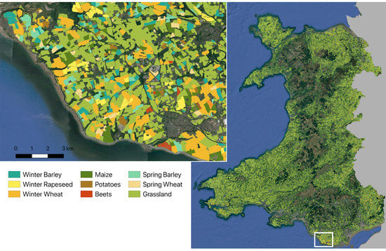
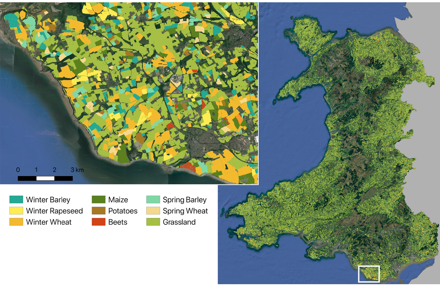
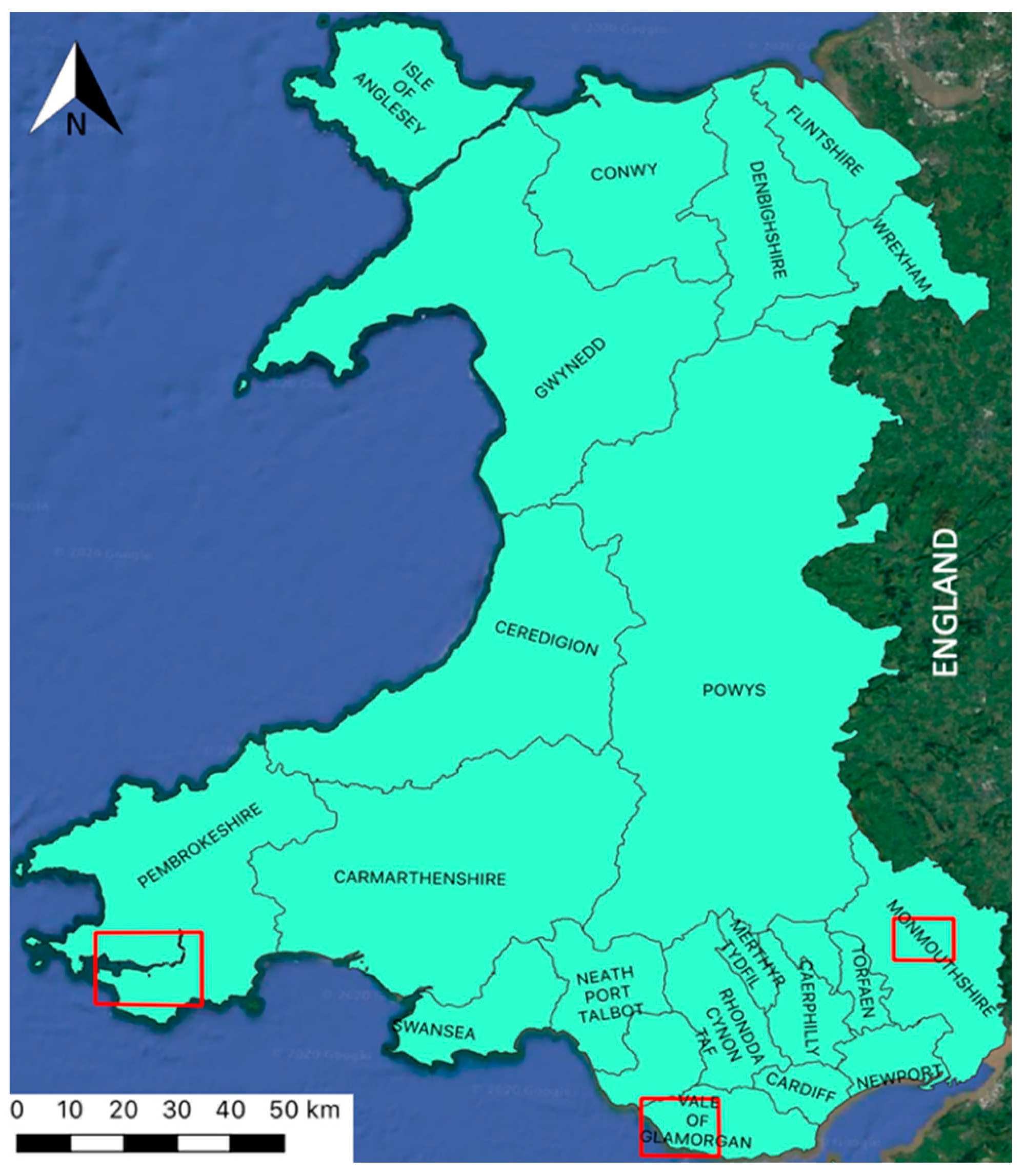
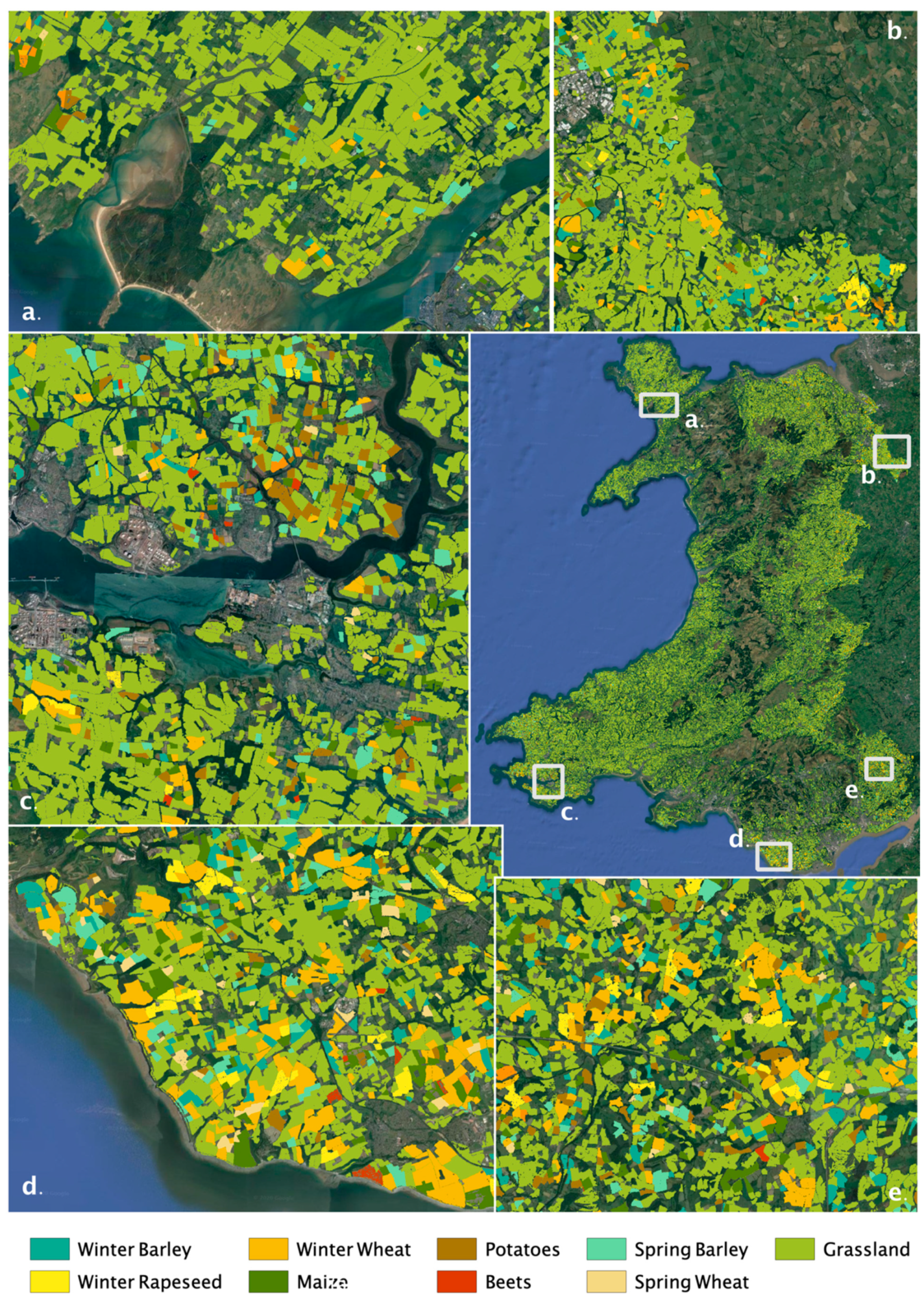
2.1. The Landscape of Wales

Wales is one of the four countries of the UK. It is a hilly/mountainous country of 20,779 km2 and much of the land is over 150 m above mean sea level, particularly in the north and center. The climate is primarily oceanic because of proximity to the Atlantic Ocean and is characterized by mild conditions (annual mean temperature of 9.5–11 °C at low altitudes), clouds that are quite persistent, particularly in the mountains, and predominantly wet (annual precipitation of 1200 mm) and windy conditions [46]. The period of greatest cloud cover is from October to the end of April, which coincides with the beginning of the growing season for several crops. However, cloud cover remains high during the whole year and as a consequence, through the major crop growth periods. December and January are the cloudier months with, on average, cloud cover higher than 40% (i.e., partly cloudy to overcast) that persists for ~80% of the time. July has more sunshine hours, but clear conditions (characterized as <20% cloud cover) occur, on average, only 24% of the time [47].
Most of Wales is vegetated and largely managed, with the uplands primarily supporting sheep grazing whilst the lowlands, particularly those in the southwest and southeast, are used for growing arable crops. A total of 88% of the land area is used for agriculture [48]. Over 75% of this area (1.332 M ha) is dominated by permanent pasture (grassland), 10% (0.180 M ha) is used for common rough grazing, and 14% (0.246 M ha) is suitable for growing crops [48]. The most commonly grown crops in Wales are spring barley (31%), winter wheat (21%), maize (18%), winter barley (10%), potatoes, spring wheat and winter rapeseed (4% each), and beets (3%). Other crop types are grown but these represent less than 1% each and 5% together. This study focused on the eight main crop types of Wales, noting that these are likely to remain as such in the future. The majority of crops are mainly located in the flat lowlands in the south, with the rest of the country being used as permanent pasture or supporting semi-natural vegetation.

2.2. Validation Sites

Sites for validating the crop type maps were selected in the main crop growing regions (i.e., Pembrokeshire, the Vale of Glamorgan, and central Monmouthshire; Figure 1). Within the three selected regions, different crop types, land management regimes, and soil/weather conditions occur.
Pembrokeshire is characterized by very complex and diverse landscapes. The north is rural with many small settlements [49]. The slopes and valleys are covered with small broadleaved woodlands and mixed or coniferous plantations but many of the flatter areas consist of a mix of fields with pasture, cereals, or hay meadows. In the south, the diverse agricultural land uses include cereal cropping, dairying, sheep rearing, and rough grazing [50]. The Pembrokeshire landscape is a mosaic of fields of varying size bounded by hedgerows, hedgerow trees, and hedgebanks. The average size of agricultural fields is 3.76 ha (4.62 ha when excluding grasslands, i.e., crops only). The agricultural area not covered by grasslands consists about equally of horticulture, winter cereals, and spring cereals [source: 2018 Land Parcel Identification System (LPIS)]. The Vale of Glamorgan is a distinctive, gentle lowland landscape, largely comprising a rolling limestone plateau with a patchwork of fields and woodlands [51]. The field sizes are larger than in Pembrokeshire, with an area average of 5.44 ha but 7.64 ha for croplands [source: 2018 LPIS]. Monmouthshire is also predominantly low lying with the landscape comprised of undulating hills, valleys, and floodplains. Sheep grazing and dairy farming are commonplace and arable farming is largely confined to the fertile floodplains. As farming is intensive, the extent of semi-natural or ecologically rich habitats is quite limited with the exception of the woodlands [52]. The average sizes of all fields and those used only for crops are 3.85 and 5.46 ha, respectively.

2.3. Data

2.3.1. Sentinel-1 C-band SAR

Sentinel-1A C-band images from 5th October 2017 to 17th November 2018 acquired over Wales were downloaded in Level-1 Ground Range Detected (GRD) format. These data were acquired in Interferometric Wideswath (IW) mode, which presents a dual polarization (VH and VV) and is the pre-defined mode over land [53]. Only data acquired in the descending orbit were used as these provided greater coverage of Wales, consistent viewing (at incident angles ranged from 30 to 46°) every 12 days at 10 m spatial resolution, and reduced processing needs. Wood et al. (2002) [54] indicated that the choice of orbit does not significantly impact on the ability to differentiate crops.
Sentinel-1 GRD products are already partially pre-processed (e.g., by multi-looking and projecting to ground range using an Earth ellipsoid model). Further pre-processing (i.e., advanced SAR calibration, geocoding and co-registration) was undertaken using the proprietary GAMMA software [55] (http://www.gamma-rs.ch/ accessed on 9 June 2020). GAMMA allows automatic and routine processing of Sentinel-1 SAR data [56]. Ticehurst et al. (2019) [57], who compared Sentinel-1 backscatters after Sentinel Application Platform SNAP [58] and GAMMA processing, found good agreement between the two. In order to improve SAR data processing, the national 2m-resolution Digital Elevation Model (DEM) distributed by National Resources Wales (NRW) on the national Lle geo-portal (http://lle.gov.wales/ accessed on 12 August 2020) was used rather than the Shuttle Radar Topography Mission (SRTM) DEM. The national DEM was obtained from airborne-LiDAR surveys carried out over several years [59]. The data were converted to backscattering coefficients (decibels; dB) and reprojected to the national coordinate reference system, the British National Grid (EPSG: 27700).
The Sentinel-1 SAR transmits and receives C-band microwaves, whose interactions with vegetation depend upon the amount and structure of plant material and also the ground conditions, including moisture and surface roughness [53]. However, the relative importance of these factors depends on the polarization, with VH and VV backscatters both influenced by the vegetation but VV being more sensitive to ground conditions. However, VH backscattering is not insensitive to soil effects. Towards the peak of the growing season, the sensitivity of SAR C-band backscattering to the ground conditions progressively decreases as crops establish and grow [60] but is greater at the beginning and end of the growing season. To reduce the effect of soil on VH backscattering, the VH/VV index was developed and used in several studies [23,53,61,62], as well as here.
In order to reduce the effect due to diversity in individual plant growth stage, this study was conducted at a parcel-based level. Kussul et al. (2016) [30] have shown that parcel- rather than pixel-based approaches allow crops to be classified with greater accuracies. In this study, and for each date, median VH, VV, and VH/VV backscattering were calculated for each parcel, with these defined using the Land Parcel Identification System (LPIS) available from the Welsh Government (see Section 2.3.2). Time series of VH/VV, VH, and VV values were then constructed for the period 5th October 2017 to 17th November 2018, which covers the crop year for Wales.

2.3.2. Land Parcel Identification System (LPIS)

The LPIS is a vector layer with associated attributes that depicts the geographic boundaries of all fields in Wales, which have been mapped through interpretation of aerial photography. The mapping is annually updated, and all fields are attributed with information on the owner, the area, and crop type, with this collected through farmers’ declarations by Rural Payments Wales. The field boundaries from the 2018 LPIS for the whole of Wales were used to generate the crop type map. The crop type data collected through farmers’ declarations were used to assess the accuracy of the resulting crop map for the three validation sites (i.e., Pembrokeshire, the Vale of Glamorgan, and Monmouthshire) (Table 1).

2.3.3. Planet CubeSat Data: PlanetScope Constellation

The PlanetScope satellite constellation consists of multiple groups of individual small satellites which have been placed in orbit through multiple launches since the end of 2016. The PlanetScope constellation captures the entire Earth’s landmass every day at 3 m spatial resolution in four different spectral bands—the visible red, green, and blue and the near infrared (NIR). In this study, the PlanetScope data available on the Planet Lab platform (https://www.planet.com/ accessed on 12 August 2020) through Planet Lab’s Ambassador Program were used to cross-check the farmers’ declarations.

2.3.4. Reference Crop Maps for Wales

For comparative purposes, the crop map generated in this study through time series analysis of the Sentinel-1 C-band SAR were compared with the two crop maps currently existing nationally for Wales. These were the UK Centre for Ecology and Hydrology (CEH) Land Cover plus [63] and OneSoil crop maps [64].
The UKCEH Land Cover plus: Crops are based on the Land Cover Map parcel framework and maps were generated for the years 2016, 2017, and 2018 by CEH. To achieve the mapping, they used an automated parcel-based crop classification algorithm, which exploited the Sentinel-1 C-band SAR and Sentinel-2 optical data. Crop maps were validated using farmers’ declarations collected by the Rural Payments Agency (for England), Rural Payments Wales, and the Scottish Government Rural Payments and Services. The CEH crop classification for Wales consists of ten classes, namely winter wheat (including oats), spring wheat, winter barley, spring barley, rapeseed, field beans, potatoes, sugar beet, maize, and improved grass, and only takes into account fields larger than 2 ha. The overall accuracy reported by CEH for the 2016 map was 87% at the UK level, but accuracies for the years 2017 and 2018 were not available at the time of this study. The accuracy assessment report highlighted that some data were missing due to the dependency of the map on the CEH Land Cover Map 2007 [65] for identifying agricultural land prior to crop classification (https://www.ceh.ac.uk/ceh-land-cover-plus-crop-map-quality-assurance, accessed on 12 August 2020).
For the OneSoil map, neural network algorithms were used to detect field boundaries and crops were then classified from Sentinel-2 optical images to generate the map. OneSoil uses in situ data provided by farmers to train its neural network algorithm and improve the accuracy of the crop maps. The algorithm was able to detect 27 crop types across Europe and the USA with (according to OneSoil) high accuracy. For Wales, the main crop types in the OneSoil map are grass, barley, wheat, maize, potatoes, sugar beet, and rapeseed. Of note is that the OneSoil map does not separate winter and spring varieties for barley and wheat. At the time of this study, maps were available for 2016, 2017, and 2018 (https://map.onesoil.ai/, accessed on 12 August 2020).

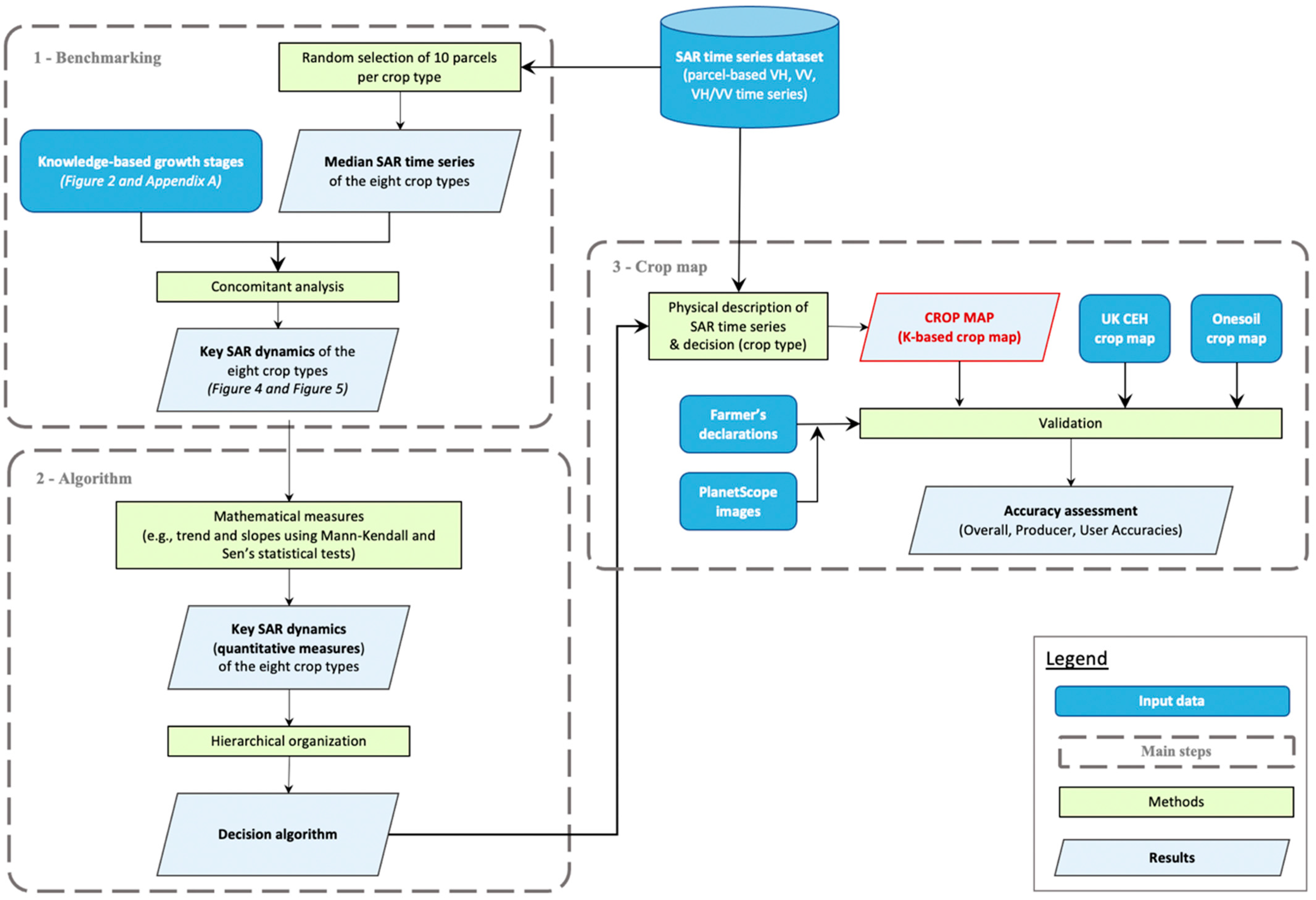
2.4. Methods for Crop Type Mapping

The methodology for classifying crop types in this study comprised three successive main steps: (a) benchmarking, (b) development of the algorithm, and (c) implementation of the algorithm to generate the crop map.

2.4.1. Benchmark Temporal SAR Dynamics

The benchmarking step consisted of a concomitant analysis of knowledge-based crop growth stages and VH, VV, and VH/VV Sentinel-1 time series to define the SAR dynamics corresponding to the key growth stages of each crop type. A range of scientific publications and various technical reports/guides, produced over past decades, give information about the average changes in biomass and other physical structures of crops, as well as the average timing of these, over Wales and the British Isles [66,67,68,69,70,71,72,73,74,75,76,77,78,79,80,81,82,83,84,85,86,87,88,89,90,91,92,93,94,95]. This study capitalized on this knowledge (i.e., theoretical/average changes in structure and timing) to undertake the benchmarking rather than relying on in situ/ground data (i.e., precise growth stage timing in the fields used for benchmarking during the whole 2018 vegetation growth period). Knowledge on growth stages and their average timings was reviewed, synthesized, and used for benchmarking of the eight crop types. This knowledge is detailed in Appendix A and summarized in Figure 2.
To determine the benchmark temporal trends in Sentinel-1 C-band backscatter for each of the eight crop types selected, VV, VH, and VH/VV time series were extracted from ten fields (per crop type) randomly selected in Pembrokeshire and median time series were calculated (see Figure 3). The resulting trends were interpreted with reference to the growth stages (knowledge-based) for each crop type (cf. Appendix A and Figure 2). From this, the uniqueness and similarities of SAR dynamics of the various crop types were analyzed, and key SAR dynamics were derived. The results (i.e., key SAR dynamics) from this benchmarking are shown and detailed in Section 3.1 and were used to support the development of the classification algorithm (see Section 2.4.2).

2.4.2. From Key SAR Dynamics to Crop Type: A Descriptive Decision Algorithm

To differentiate and map the different crop types from temporal SAR data, a decision algorithm was developed.
(a) Key SAR dynamics (mathematical measures)
First, the key SAR dynamics resulting from the benchmarking (see results in Section 3.1) were translated into quantifiable variables using mathematical measures, namely magnitude, noise, trend, and slope (see Figure 3 and Appendix B).
In order to measure trends (e.g., increase or decrease), Mann–Kendall and Sen’s slope statistical tests were used over the key SAR dynamics’ periods. The Mann–Kendall (MK) test [96,97] is a rank-based non-parametric statistical trend test which has been widely used to detect significant monotonic trends and changes in time series (e.g., [98,99,100,101,102,103,104]). One of the main advantages of this statistical test is that, compared with parametric statistical tests, it is more suitable for non-normally distributed data, which are frequently encountered with environmental variables [105]. The MK test has been used mainly for analyzing time series of climatic and environmental data, but any type of data can be evaluated. Recently, Dabrowska-Zielinska et al. (2018) [106] used MK to interpret time series of Sentinel-1 C-band SAR for estimating soil moisture variations over wetlands. In this study, a p-value of 0.01 was used in the MK test to determine trend significance. Trends with p-value > 0.01 were considered not significant (c.f., M K n o in Appendix B). Following detection of a significant trend by the MK test, Sen’s slope test [107,108,109] was used to measure the orientation of the slope (i.e., positive/negative) and quantify magnitude (c.f., S s l + , S s l , and Mag in Appendix B). Sen’s slope is a non-parametric test which is based on the median slope rather than the mean slope (as in the case of parametric linear regression). Note that, even though these two tests are based on a monotonic trend hypothesis, the presence of outliers does not decrease their relevance [110,111,112], as they are non-parametric tests. Hamed (2008) [111] mentioned that the use of non-parametric trend tests is more suitable for detecting trends in time series which may contain outliers.
Finally, in order to measure noise, the average difference between original values and smoothed values during the key SAR dynamics period was calculated and used. Smoothed values were calculated using locally weighted least squares regression (i.e., loess) [113,114] which combines the simplicity of the classical least squares method with the flexibility of non-linear regression [115]. It is a non-parametric method where least squares regression is performed in localized subsets, which renders it a suitable candidate for smoothing volatile time series. It has been widely used in the literature to smooth curves and filter noise in various types of dataset e.g., [116,117,118,119,120]. In this study, we used loess to detect if noise occurred during the key SAR dynamics’ periods. “No noise” (c.f., N s e n o in Appendix B) was attributed where an average difference of ~0 dB was found between original values and smoothed values during the analyzed period.
(b) Decision algorithm
The key SAR dynamics (mathematical measures) were hierarchically organized in order to develop a conditional decision algorithm. The hierarchical organization in the algorithm was defined after analysis of the uniqueness and similarities of the key SAR dynamics resulting from the benchmarking (see Section 3.1), and is detailed in Appendix B. The developed algorithm allows (a) a physical description of the temporal SAR time series of fields using the previously mentioned mathematical measures over key analysis periods, and then (b) makes decisions regarding the crop type based on conditional decisions (c.f., Appendix B). The key analysis periods used by the algorithm are based on knowledge of the different growth stages (see Figure 2) and the analysis of the results of the benchmarking (see Section 3.1 and Section 4). In the algorithm, first, long periods (i.e., the beginning of November to the end of March and the beginning of April to the end of the growing season) are used by the algorithm to make decisions regarding the broad crop category (i.e., winter and spring crops), c.f. Appendix B. Then, using shorter periods (i.e., 2 months and 1 month) and the mathematical conditions listed in Appendix B, decisions regarding the crop type are made (i.e., wheat, rapeseed, and barley for winter crops or potatoes, barley, maize, beets, and wheat for spring crops). The grassland category is assigned when none of the mathematical conditions are met.

2.4.3. Generation and Validation of Crop Map

The third step is algorithm implementation which allowed generation of the crop type map for Wales. The classification of crop types was confined to the cultivated/managed vegetated area of Wales. For each of the LPIS parcels within the cultivated/managed vegetated area, the decision algorithm was applied to the parcel VH/VV, VH, and VV time series in order to generate the crop map (see Figure 3). The grassland category was assigned to parcels that exhibited no key temporal signature in the Sentinel-1 C-band SAR time series.
Whilst the decision algorithm was applied at a national level, the classification was validated for the main agricultural regions of Pembrokeshire, the Vale of Glamorgan, and Monmouthshire using the crop types declared by farmers for each of the LPIS parcels. As the farmers’ declarations may contain errors, they were cross-checked through visual interpretation of the very high resolution and temporal frequency PlanetScope images acquired over the study period. Parcels were discarded where the declared crop type was different from that observed in the PlanetScope imagery or was not listed as one of the eight studied crop types (or grassland). For Pembrokeshire, fields used for benchmarking were removed. The size of the validation samples within each agricultural area was similar (Table 2). For each area, confusion matrices were generated, and a range of metrics for quantifying accuracy were calculated, including overall accuracy (OA), omission and commission errors, and producer and user accuracies (respectively, PA and UA). As concerns have been raised about the use of the kappa agreement [121,122,123,124,125,126,127], this measure was not used in this study.
Although these three regions were selected because they were the main arable areas of Wales, grassland remained the predominant cover, accounting for approximatively 60% to 70% (see Table 1). When trying to quantify the accuracy of land cover maps, the total size of the validation sample and the proportion of each class within that sample are of great importance. Allocating approximately equal sample sizes to each class is a relatively common practice in accuracy assessment [125] and allows approximately equal precision for the estimated user’s accuracy of each class to be provided. However, larger sample sizes can be allocated to specific classes depending on the objectives. This study aimed to classify crop types in cultivated/managed vegetated areas at a national level and hence, over large areas.
To validate the capacity of the method to accurately classify the cultivated landscape, accuracy was first assessed using samples where the proportion of each class was representative of those occurring in the landscape (i.e., including grassland). For this purpose, we used a systematic selection method, as it allows more precise estimates [127]. Secondly, to determine the capacity of the method to distinguish the different crop types, accuracy was estimated using normalized confusion matrices containing only the eight crop types (i.e., excluding grassland). At the same time, and using the same validation samples and method, the accuracy of the other national crop maps for Wales (i.e., CEH and OneSoil) was assessed for comparative purposes (Figure 3).

3. Results

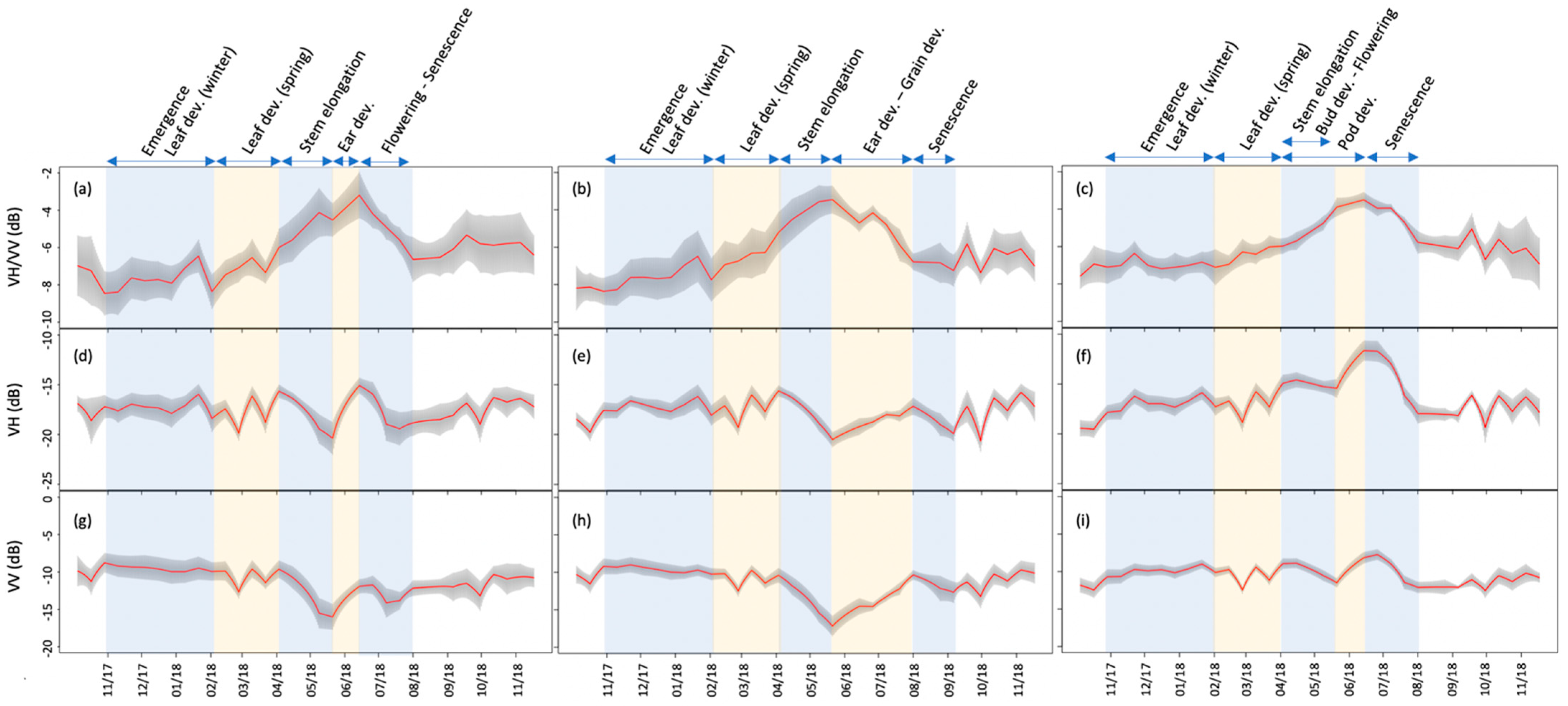
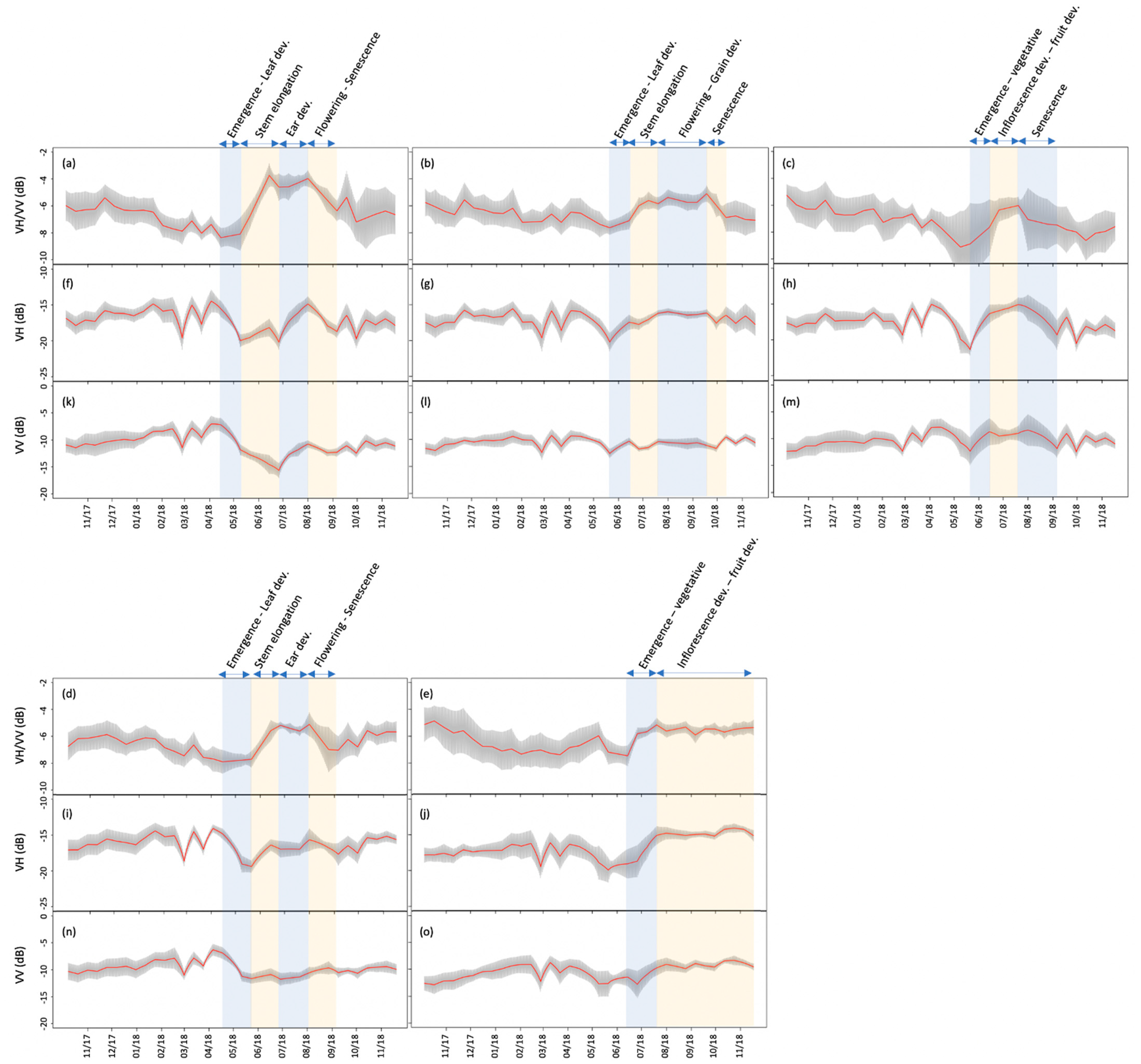
3.1. Key Temporal SAR Signatures (VH/VV, VH, and VV)

The benchmarking exercise identified differences in the temporal C-band VH, VV, and VH/VV signatures of both winter and spring crops (Figure 4 and Figure 5) which could be interpreted through reference to the knowledge-based crop growth stages (GS), cf. Figure 2 and Appendix A.

3.1.1. Winter Crops

All three winter crops (i.e., barley, wheat, and rapeseed) exhibited a slow but slightly increasing value of VH/VV during November, December, and January, with this corresponding to winter emergence and leaf development (Figure 4). From February, a more rapid increase in the VH/VV marked the beginning of the spring component of the leaf-development phase, which continued until the beginning of April. By comparison, the spring crops (Figure 5) exhibited a decreasing or largely stable trend in the VH/VV from the beginning of November to the beginning of April. Thereafter, a rapid increase in the VH/VV slope was observed in winter crops, with this corresponding to a period of stem elongation (cf. Figure 2). Maximum VH/VV was observed during May or June, with this varying by species. Wheat attained its maximum VH/VV around mid-May (maximum of ~−3 dB) whilst barley and rapeseed were around mid-June (with values of −3 and −4 dB, respectively). The observations concurred with the knowledge-based GS periods for these species (cf. Figure 2).
A dynamic response was also observed in the VH time series, which corresponded with distinct periods during the crop growth and phenological cycle. For wheat (Figure 4), when the VH/VV reached a maximum (i.e., around mid-May), the VH started to increase until the beginning of August. For barley, the VH increase commenced around mid-May (i.e., before the maximum of the VV/VH) and the maximum was reached at the same time as the maximum VH/VV (i.e., mid-June). Hence, the timing of the VH increase aligned differently with the VH/VV dynamics for wheat and barley. Reference to the knowledge-based GS (Appendix A) indicated that this change aligned with the different inflorescence emergence time for barley and wheat crops. The increase in VH also occurred over a shorter period for barley compared to wheat and hence, the slope was steeper.
As with barley, rapeseed exhibited a marked increase in VH between mid-May and mid-June and the maximum occurred at the same time as the VH/VV. However, contrary to barley and wheat, which showed an important decrease in VH between the beginning of April and mid-May, rapeseed VH almost plateaued (Figure 4). According to the knowledge-based GS, this occurred during the concomitant occurrence of stem elongation with bud development and flowering. This led to high VH values (i.e., −15 dB) around mid-May in rapeseed fields compared to the other winter crops (i.e., around −20 dB). As VH values are already high around mid-May and further increase until mid-June, maximum VH is largely higher in rapeseed’s field plots compared to barley’s or wheat’s, respectively, −11, −15, and −17 dB. These are the key dynamics that allowed us to distinguish barley, wheat, and rapeseed (see Appendix B). The shape of the VV signal was similar to VH throughout the time series but the magnitude varied because of different interaction with the plant components. These differences were reflected in the dynamics observed in the VH/VV ratio.

3.1.2. Spring Crops

The time series of VH/VV, VH, and VV for the spring crops of barley, wheat, maize, potatoes, and beets also showed a dynamic seasonal signal (Figure 5), which reflected different components of the crop cycle identified in the key knowledge-based GS. The temporal signatures for winter and spring barley were similar, with the VH/VV again showing a slow gain from mid-April to the beginning of May and steeply increasing thereafter to a maximum around mid-June. The VH time series was characterized by a steep increase for one month (i.e., during July) followed by a decrease which started at the same time as the VH/VV decrease (i.e., August). However, contrary to winter barley, which showed an increase in VH/VV in parallel to the VH increase, spring barley’s VH/VV time series was marked by a plateau. Reference to the knowledge-based GS indicated that this corresponded to the period when canopy size plateaus soon after flag leaf emergence until the spring barley ears are fully developed (Appendix A and Figure 2). The maximum VH/VV value for spring barley was 20% lower compared to the winter variety. The knowledge-based GS also indicated that the peak canopy size was, on average, 15–20% less for spring barley [78,88]. As with spring barley, spring wheat exhibited a plateau in the VH/VV time series during July and a lower maximum VH/VV value compared to the winter variety, but a smaller increase in VH was found compared to barley during the ear development (~1.5 and ~5 dB, respectively).
For potatoes, a high variability in VH/VV between fields was observed throughout the entire growing season (Figure 5), which presented limited opportunities for discrimination. However, from the median VH/VV, three phases identified in the knowledge-based GS (vegetative, reproductive with maintenance of green parts, and reproductive with senescence of green parts) could be associated with steep and less steep increases and a decrease in values, respectively. These phases were also evident in the VH time series, and with a low standard deviation in each time step. Of note was that potatoes displayed a large increase in VH similarly to spring barley (~5 dB) followed by a decrease of ~3 dB. However, for potatoes, the VH increase commenced in mid-May (rather than the beginning of July for barley), with this leading to a comparatively longer period of increasing VH (i.e., two rather than one month). Furthermore, a corresponding increase in VV with VH was observed whilst, for spring barley, a decrease in VV occurred during that period.
For maize, two periods of growth can be distinguished, with a slower and subsequent steeper increase corresponding to the emergence and development of the first leaves and period of stem elongation, respectively (cf. Figure 2). As with beet, the VH/VV and VH of maize plateaued from July to September but whilst this continued for beet, a decrease in VH/VV occurred from mid-September to mid-October in maize crops. Additionally, in contrast to maize, the VV of beets increased and then plateaued. Throughout the growing season, the VH/VV increase was significantly lower (~2 dB) for maize compared to other cereals (at least 4 dB).

3.2. A Crop Map for Wales

On the basis of the median VH/VV, VV, and VH time series, key SAR dynamics for discrimination of spring and winter barley and wheat, winter rapeseed, maize, potatoes, and beets were identified (see Section 3.1) and translated to quantifiable mathematical measures and a decision algorithm (see Appendix B) allowing crop mapping for each field in Wales. These were defined by the Welsh Government LPIS within the cultivated/managed landscape. Each of the functions of the algorithm was associated with a description of the crop phases obtained through reference to the knowledge-based GS.
The mapping captures the extent of crop lands as well as grasslands in agricultural Wales landscape and estimated that 86.1% of cultivated/managed area is covered by grasslands, with the remainder occupied by maize (21.7%), winter wheat (19.6%), spring barley (18.5%), winter barley (17.4%), potatoes (10.6%), spring wheat (7.75%), rapeseed (3%), and beets (1.5%). The national map and subsets of the map, showing the extent of cultivated crops and grasslands, are given in Figure 6.
The accuracy of the crop and grassland map was quantified for Pembrokeshire, the Vale of Glamorgan, and Monmouthshire using the datasets presented in Section 2.4.3 and Table 2. Overall accuracies (OA) (Table 3) were also generated for the CEH and OneSoil crop maps using the same validation datasets. At the agricultural landscape level (i.e., including grassland, “all parcels” in Table 3) and for all validation sites, the OA ranged from 82.0% to 90.2% when using the knowledge-based proposed methodology (i.e., mentioned K-based map in the rest of the paper). When winter and spring varieties (i.e., “seasonal crops” in Table 3) as well as grasslands (i.e., “all parcels” in Table 3) were considered, the highest OAs for Pembrokeshire (90.2%), the Vale of Glamorgan (89.6%), and Monmouthshire (82.0%) were all obtained with the K-based map. With the exception of Monmouthshire (92.2% with OneSoil), the K-based map also displayed the highest accuracies when considering grasslands and crops, with no distinction between winter and spring varieties (i.e., “annual crops” in Table 3). Over the three areas, regardless the product, grassland showed user accuracies (UA) greater than 95%, with only the exception of CEH in Pembrokeshire (i.e., 84.7%), not shown here.
Using normalized confusion matrices containing each crop type and excluding grasslands (i.e., labelled as “crops” in Table 3), the capacity of the proposed methodology to classify crop types was evaluated and compared to other maps available for Wales (CEH and OneSoil). With the exception of Monmouthshire, where the CEH map OA was ~94%, the K-based map showed higher accuracy with OA ranging between 85.8% and 90.6% (Table 3).
The omission and commission errors as well as the producer and user accuracies (PAs and UAs, respectively) of each of the crop types for the K-based, CEH, and OneSoil maps were quantified, using normalized confusion matrices containing each crop type and excluding grasslands. Depending on the region, the crops types differ. Only the crop types with a significant number of parcels were analyzed. In the three validation areas, the number of beets and spring wheat field plots was too small to be considered in the accuracy analysis. Potatoes fields were significantly present in Pembrokeshire but not in the two other regions and very few spring barley fields were present in Monmouthshire.
For Pembrokeshire, the K-based map provided higher PAs for five of the six crop types considered, with the exception of potatoes (79% compared to 100% for CEH; Table 4). PAs exceeded 90% for winter barley, winter rapeseed, and maize and 80% for winter wheat and spring barley in the K-based map (see Table 4). Winter barley and winter rapeseed also displayed accuracies greater than 90% in the CEH product. However, the CEH PAs for winter wheat and spring barley were less than 80% (respectively, 65.96% and 77.78%). Compared to the K-based and CEH maps, OneSoil performed very poorly in the Pembrokeshire region with PAs of 45.24%, 50.00%, and 62.07%, respectively, for wheat, potatoes, and barley and UAs of 57.21% and 63.78% for barley and maize (see Table 5). In the Vale of Glamorgan, the PA for all crops was > 80% for the K-based map, with the exception of maize (at 77%). The CEH PA for spring barley was very low because of high misclassification to spring wheat and the UA was low because of a commission error of 39.7% from winter wheat. Similarly, poor results in the OneSoil map in this region came from a confusion between barley and wheat, leading to a wheat PA of 59.29% and a barley UA of 61.24%. For Monmouthshire, within the K-based product, only the maize PA was under 80% (i.e., ~76%). In both Monmouthshire and the Vale of Glamorgan, this <80% maize PA was attributed to misclassification of maize into several other but not any specific crop types. In Pembrokeshire, the PA for maize was 90.0%, suggesting that other factors (than the algorithms) might be contributing to the map accuracy (e.g., parcel size, mixed SAR signal).
For all fields and regardless of their location, the OAs and PAs were analyzed by field size (Figure 7a,b). The accuracies increased with field size up to an area of 8 ha (Figure 7b) but then remained relatively similar thereafter. This was especially the case for the spring varieties. Maize and spring barley, which had the lowest accuracies in the K-based map (see Table 4), respectively increased from 60.0% to 83.3% and 50.0% to 100.0%, for fields that were on average <2 to 8 ha (Figure 7b). This led to an increasing OA in the K-based map as field size increases (Figure 7a).

4. Discussion

By using knowledge gathered by the agricultural community to inform a descriptive decision algorithm based on the Sentinel-1 C-band SAR time series, eight different crop types were able to be mapped across Wales for 2018 with overall accuracies of between 85.8% and 90.6% depending on the area. The classifications were generated without the use of in situ/ground training datasets nor machine learning but provided accuracies that exceeded those of other products that included these techniques in their mapping. The concomitant analysis of knowledge-based GS and time series of VH, VV, and VH/VV Sentinel-1 C-band SAR data allowed interpretation of signatures through biophysical meaning. The VH/VV trends were similar to those observed in the knowledge-based GS and particularly related to changes in canopy size (see Figure 2). This is consistent with several previous studies (e.g., [53]) that have shown that the VH/VV ratio is correlated with fresh (green) biomass. As the VH/VV ratio reduces sensitivity to soil effects, as observed with VH and VV, detection of slow and small trends in vegetation growth during the winter season (barley, wheat, and rapeseed) was discerned. This allowed us to separate winter and spring crops with very high accuracy (> 95%).
With the start of spring, winter crops display an increase in the VH/VV because of the increase in fresh biomass through leaf production. Winter barley and wheat both displayed a large decrease in VH and VV during the stem elongation stage. These trends are consistent with the literature and seem to occur during this growth stage regardless of the European region and period. Veloso et al. [53] in the southwest of France during 2015 and Khabbazan et al. [23] in their study case in the Netherlands during 2017 found similar trends for barley and wheat crops. The decreases in VH and VV during stem elongation are both induced by vegetation rapid growth, but for different physical reasons. Whereas the VV signal is dominated by both direct ground and canopy contributions, VH is influenced by double-bounce scattering between the stem and ground, as well as by volume scattering [53,128]. Hence, the VV decrease is attributed to the increasing attenuation of the vertically polarized wave led by the growing vertical structure of cereals on both forward and return propagation paths [23,53,129,130]. As stems elongate, the double-bounce and the volume fraction of the vegetation change, which affects the VH.
During the second part of May, VH and VV start to increase. The difference of timing alignment between VH and VV trends and maximum VH/VV for barley suggests (from the knowledge-based GS) a contribution from inflorescence (i.e., ear) development. Indeed, barley and wheat have a very similar structure, but one of the major differences is that winter barley reaches its maximum green biomass at the end of the ear emergence, whereas wheat’s maximum canopy size occurs between flag leaf emergence and ear emergence [78,87,88]. Khabbazan et al. (2019) [23], who compared the time series of Sentinel-1 backscatter with ground measurements, mentioned that VV increase in winter wheat is due to flag leaves and/or inflorescence emergence, with this supported by Mattia et al. (2003) [60]. Similarly, Veloso et al. (2017) [53], who analyzed the temporal behavior of Sentinel-1 C-band backscatter in a field plot of winter barley, related this phenomenon to heading (i.e., inflorescence emergence). Note that inflorescence development also leads to increasing fresh biomass in barley but not in wheat crops. This induced an increase in VH/VV for barley fields but not for wheat, strengthening the correlation between the ratio and fresh biomass and showing the importance of the inflorescence emergence period to distinguish barley from wheat.
Contrary to winter cereals, in rapeseed crops, the VH and VV signals approximately followed the same temporal dynamics as the VH/VV signal. Unlike barley and wheat, rapeseed does not display a large decrease in VH but instead, slightly decreases and almost plateaus. According to the knowledge-based GS, this occurs during the concomitant occurrence of stem elongation with bud development and flowering. Fieuzal et al. (2013) [62] and Wiseman et al. (2014) [131] observed a similar trend in the RADARSAT-2 C-band VH data. They showed that the minimum of the small decrease in VH is reached when flowering is occurring, which agrees with our results. As pods develop, VH shows a steep increase and the increasing VH/VV rate lowers. As no predominant orientation exists, volume scattering increases, which explains the increase in VH during that period [62].
In most crops, VH/VV is generally well correlated with fresh biomass and this allowed detection of a ~20% lower biomass in the spring variety compared to the winter variety of barley, which is commonly reported in the literature [78,88]. However, in potato crops, VH was found to be of greater use, as the VH/VV displayed large standard deviations during almost the entire growing season but particularly just before and during the emergence and vegetative stages. This sudden increase in the standard deviation of VH/VV from mid-April (i.e., the planting period) was largely due to greater sensitivity of the VV backscatter compared to the VH. The standard deviation decreased as the VH/VV (fresh biomass) increased, with minimal standard deviation obtained at maximum canopy size. Hence, the high variation in the VH/VV during the first stages of potato growth was probably due to the soil ridges within which the potato crops are planted. Differences in the orientation of the ridges with respect to the radar viewing direction result in variations in the backscatter from bare soil [23]. As mentioned in the literature, VV is more sensitive than VH to directional scattering induced by ridge and/or row orientation [23,128,132,133] and sensitivity decreases as canopy covers bare soil.
For maize, the changes in VH/VV mirrored those in canopy size given by the knowledge-based GS. The VH displayed a similar trend to VH/VV. However, contrary to other crops where VV follows a similar trend as VH, in maize, the VV time series remained flattened during the growing season. This absence of a correlation between the VV and the biomass in maize crops has been reported in the literature [23]. Vreugdenhil et al. (2018) [134], who studied the sensitivity of Sentinel-1 C-band backscatter to vegetation dynamics using in situ reference data in Austria, showed that VV backscatter is mainly sensitive to soil moisture in maize crops due to the distance between maize rows. As row spacings are generally large (i.e., ~70 cm), the VV is still influenced by direct ground contribution until late stages, which leads to a poor correlation with biomass. Additionally, whereas the VH/VV trends accurately matched the changes in biomass, we noticed that just before emergence, the VH/VV for maize was higher than other crops. This led to a 2 dB increase during the growing season, which contrasted with the (at least) 4 dB of winter crops. Some potato fields also displayed a high VH/VV at the beginning of the growing season and this was attributed to the establishment of the soil ridges and their arrangement in rows. However, for potatoes, this period was also associated with high variability in VH/VV between the fields, which was not the case with maize crops. Moreover, no such phenomenon has been reported in the literature. In this study, the small change in the VH/VV for maize during the growing season can be explained by the configuration of the landscape. In Pembrokeshire, where benchmarking field plots were selected, the multiple small fields (3.76 ha on average) form a mosaic bounded by hedgerows and hedgerow trees [50]. During the second part of May (i.e., the period of maize emergence), the semi-natural vegetation (including hedgerows and hedgerow trees) is fully developed, which influences the parcel-based averaged SAR backscatter. Trees have a VH/VV value of ~−5 dB during that period, which could explain the high VH/VV of late crops such as maize.
Compared to studies analyzing the Sentinel-1 time series using in situ/ground measurements, very similar results based on knowledge acquired from various technical reports were observed. In this study, it has been shown that knowledge-based growth stages can be used to interpret and detect key dynamics in SAR time series. The concomitant analysis of knowledge-based crop growth stages and average Sentinel-1 C-band time series allowed us to understand the temporal dynamics of the C-band SAR observations for the eight main crop types. In general, VH/VV and VH were shown to be the most correlated to changes in vegetation structure during the growing season and, thus, were the two most important variables for defining the key dynamics. From this benchmarking, translation into quantitatively measurable variables was possible, with this leading to the development of the descriptive decision algorithm. Using this algorithm on parcel-based Sentinel-1 time series allowed mapping of crop types across Wales with an OA exceeding 85% in the majority of cases.
Two methods were used to evaluate the crop map, with the first using samples where the proportion of each class was representative of the landscape (i.e., grasslands were included) and the second considering the crops only and using equal sample sizes for each class. Overall, the accuracies were comparable and often exceeded those obtained for the CEH and OneSoil maps, and the K-based product was found to be more consistent. The OneSoil map achieved a high level of classification accuracy in the mapping of grasslands and hence, a large overall accuracy, but different crop types were not able to be discriminated to the same level as with K-based. By contrast, CEH showed good capacity to distinguish crop types, but the overall accuracy at the landscape level was lower (i.e., 60% to 70%) due to the high number of missing data. The K-based product provided accuracies that were generally > 85% overall for both classifying the agricultural landscape and distinguishing crop types. In terms of crop types, it was particularly effective in distinguishing barley from wheat. Confusion between these two crop types is a major source of error in the other two map products but distinction was achieved by the K-based classifier, which capitalizes on the knowledge of the different growth stages of the two species.
In general, the accuracy in the mapping of spring crops was lower than that of winter crops. Accuracies were also found to be a function of field size, which partially explains this outcome. The Welsh landscape is characteristically a mosaic of small fields bounded by hedgerows and hedgerow trees. Giordano et al. (2018) [32], who proposed a parcel-based methodology allowing crop type mapping from a sequence of satellite acquisitions (radar and optical), also demonstrated a high sensitivity of radar images to parcel size, especially in fragmented landscapes. The GRD Sentinel-1 data were similarly used as input data. As the pixels of the GRD product are averages of five pixels of the Single Look Complex (SLC) product, they suggested the use of SLC images in order to improve the accuracy of classification, as well as the use of a high-resolution Digital Terrain Model instead of the SRTM. Radar speckle filtering was also mentioned as a potential source of error in small objects. Of note is that the SAR processing in this study utilizes a national 2m-resolution Digital Elevation Model (DEM).
The size of parcels can only partially explain differences in the accuracies obtained as winter and spring crops generally do not have significantly different field sizes. Figure 7b highlighted that whilst all crop types are sensitive to parcel size, spring crops are affected in a stronger way. Semi-natural elements (e.g., hedgerows, hedgerow trees, and grass strips) can contribute to the signal and the overall response from a field. This is most likely to occur during late April–May, when some of the spring crops emerge whilst semi-natural elements have already started to develop (e.g., through growth and leaf flush). The smaller the parcel, the higher the effect of edge elements is likely to be, with this resulting in a lowering of accuracy. As the first growth stages are crucial for the classification of crop types, noise in the SAR signal during that period is likely to introduce error. Errors are, therefore, likely to be greater for small parcels of spring crops surrounded by hedgerows or hedgerow trees. Denize et al. (2019) [135] mentioned hedgerows as noisy features in land use mapping and removed them from the images using a 5 m negative buffer. A similar method was tried in this study, but the remaining area within the parcels was too small to clearly characterize key SAR dynamics.
Despite these limitations, the knowledge-based descriptive decision algorithm provided crop and grassland maps with an accuracy that was similar but often improved over those provided by CEH or OneSoil. The K-based method is more consistent in that it provides less variability between classes and regions compared to the other maps. This is due to both the type of data and algorithms used in this study. Timing is very important when addressing the issue of crop type mapping. In this study, we used only SAR time series. A particular advantage of SAR in regions with frequent cloud cover, including Wales, is the ability to obtain a complete time series from the images that are available. As such, all growth stages can be captured because of observations throughout an annual cycle, and the quality during the whole year and over the whole study area remains the same, regardless of local weather. The maps generated by OneSoil and CEH relied, respectively, totally or partially on optical data, which would have introduced discrepancies in the final product because of missing data and/or perpetual change in the proportion of optical data used and their quality, due to clouds.
The proposed approach also provides more consistent mapping as it allows tailoring to regional and/or local land management and weather/soil/plant conditions. The use of the MK non-parametric statistical trend and Sen’s slope tests ensures that the approach is robust to a few outliers and the developed algorithm is sufficiently flexible to account for temporal shifts in growth patterns as a result of regional/local weather, soil condition, plant stress, and/or timing of crop management actions. In this study, 12-day temporal frequency data were used. A delay of one date in the time series (i.e., one outlier) is, therefore, a shift of 12 days in the growing season. In many parts of Europe, between years and regions, the growing season is usually shifted by a maximum of one month. For example, Khabbazan et al. [23] showed a shift of less than two weeks for maize, potatoes, and winter wheat crops in the Netherlands during 2017 compared to Wales in 2018. Similarly, Veloso et al. [53] and Vreugdenhil et al. [134], respectively, showed a shift of (approximatively) one month in southwest France during 2015 and two weeks in Austria during 2017 compared to the growing season observed for Wales. By tolerating a few outliers, the accuracy of the final product displayed no correlation with the distance to benchmarking field plots, therefore allowing the system to be consistent when mapping crops in different regions of Wales. This also glimpses the potential of the proposed method for mapping crop types over other large areas and potentially several countries or regions in Europe.

5. Conclusions

For crop mapping over large areas, a consistent and flexible descriptive knowledge-based (K-based) algorithm that solely used Sentinel-1 C-band SAR annual time series has been developed, with this being informed by knowledge gathered by the agricultural community on crop growth stages. The method was developed for Wales and the accuracies of classification are comparable or exceed those generated in previous efforts, with these based on optical or combined SAR-optical data. As Wales is frequently covered with clouds, the use of Sentinel-1 C-band data alone is advantageous as scenes are currently available at a national level every 12 days (when using one orbit), which allows consistent application and outputs for all regions.
In general, VH/VV and VH were shown to be the most correlated to changes in vegetation structure during the growing season and, thus, were the two most important variables for crop type mapping. Whereas the VH/VV ratio has shown to be very correlated with canopy size (i.e., fresh biomass), VH shows especially good capacity to detect inflorescence (i.e., ears) emergence in winter cereals. Wheat and barley have a very similar structure but timing alignment between the beginning of the VH increase (i.e., ear emergence) and the maximum VH/VV (i.e., maximum green biomass) is different, with this period being crucial for separating wheat from barley. By capitalizing on this fundamental difference, these two crop types were particularly well differentiated, which is a significant advance given these are not well captured in other products available for Wales. The accuracies of classification, however, varied as a function of field size in this parcel-based approach and increased progressively up to an area of 8 ha but then remained relatively similar thereafter. This was attributed to contributions from structures located on the boundaries of fields, which generally increase with decreasing parcel size. The edge effect was especially evident in spring crop fields. Foliage production in hedgerows and/or hedgerow trees (i.e., semi-natural elements of the landscape) has generally already started when spring crops emerge. This introduces noise in the overall SAR response during the first crop growth stages, which are critical for crop type mapping.
Despite the size effect and the small size of plots in Wales, the overall accuracies of crop type mapping using the proposed method were between 85.8% and 90.6%. Compared to other methods that have been used for crop mapping in Wales, the developed method was more consistent as variability in accuracies between classes and regions was lower. This was attributed largely to the sole use of Sentinel-1 C-band data, without dependence on optical data, but the algorithms used in the method also played a key role in the consistency. The Mann–Kendall non-parametric statistical trend and Sen’s slope tests ensured that the approach was robust to a few outliers and was sufficiently flexible to account for temporal shifts in growth patterns as a result of regional/local weather/soil/plant conditions and timing of crop management actions. By tolerating a few outliers, the accuracy of the final product displayed no correlation with the distance to benchmarking field plots, therefore allowing the system to be consistent when mapping crops in different regions.
By relying on (a) Sentinel-1 C-band data only, (b) knowledge, and (c) flexible algorithms, the proposed method has shown to be a good alternative for consistent and accurate crop mapping over large areas with persistent cloud, where access to in situ/ground information and optical data was not be easy to obtain. The method was applied at the national level in Wales, but this study also foresees the potential of the method for mapping crop types over other areas and potentially several countries or regions in Europe.

Author Contributions

Conceptualization, C.P. and R.L.; methodology, C.P.; validation, C.P. and C.H. (Clive Hurford); writing—original draft preparation, C.P.; writing—review and editing, R.L., S.P., S.C. and C.O.; resources, C.H. (Claire Horton) and P.G.; data curation, S.K. and S.W.; supervision, R.L. and P.B. All authors have read and agreed to the published version of the manuscript.

Funding

This research was funded by the European Research Development Fund (ERDF) Sêr Cymru II program award (80761-AU-108; Living Wales).

Acknowledgments

The authors would like to acknowledge PlanetLab for allowing access to the PlanetScope data for Wales, as well as the Welsh Government for making 2018 LPIS data and farmer’s declarations available.

Conflicts of Interest

The authors declare no conflict of interest. The funders had no role in the design of the study; in the collection, analyses, or interpretation of data; in the writing of the manuscript, or in the decision to publish the results.

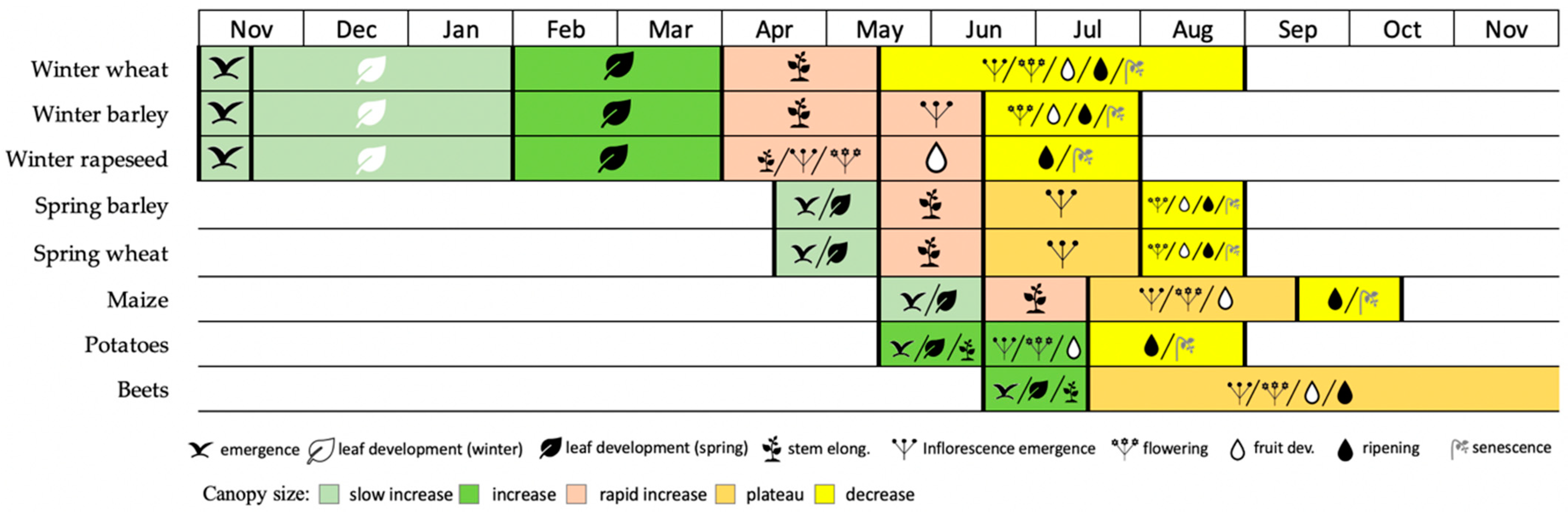
Appendix A. Knowledge-Based Growth Stages

Appendix A.1. Winter Wheat

Winter wheat growth is composed of over ninety stages, starting with germination and ending with senescence, which are fully described and explained in various technical reports [83,87,90]. In Wales, winter wheat is sown during the early autumn of year-1 (Y-1), leaves start emerging during November, and the leaf emergence and tillering stages last the whole winter [68]. As the development of plants is mainly governed by the temperatures and the photoperiod, establishment of the winter crops is slow. From February–March, with the increase in temperatures and length of days, the rate of vegetation growth increases. Growth during early development stages is mainly driven by leaf formation; by the start of the stem extension stage, which occurs around April, the crops have produced most of their leaf biomass [83]. During the stem extension stage, canopy expansion is rapid as stems elongate and canopy biomass typically reaches its maximum before anthesis. Indeed, reports mention that “maximum canopy size occurs between flag leaf emergence and ear emergence” [87]. After stems are fully extended, canopy expansion stops, and the amount of green biomass starts to decline due to senescence.

Appendix A.2. Winter Barley

As with winter wheat, winter barley growth is composed of over ninety stages, starting with germination and ending with senescence. In general, winter barley growth stages (GS) are very similar to winter wheat [90]. Indeed, similarly, in Wales, winter barley is sown during the early autumn of Y-1 and early development stages have a slow growing rate as they occur during winter [68]. From February–March, the rate of leaf development starts to increase and, from April, canopy expansion accelerates as (1) tillering and leaf emergence continue and (2) stem elongation starts. Increase in canopy biomass and height continues until ear emergence and flowering stages. However, contrary to winter wheat, for which maximum green biomass occurs before ear emergence (end of stem extension), barley reaches its maximum at the end of the ear emergence stage (due to their greater surface due to awns) [78,88]. The ears of barley, which are composed of long awns, play a very significant role as they represent 11% of the green area [95]. Then, as grain filling begins, heads start to bend and lower leaves to die, leading to a decrease in green biomass [78,88]. Barley generally has weaker stems than wheat. The crop is more susceptible to stem lodging at the base as well as necking further up the plant. Heads bend early in the season when grain watery ripe starts.

Appendix A.3. Winter Rapeseed

As the two crop types previously described, winter rapeseed is sown during the autumn. Leaf production starts before the winter with a slow growth rate and accelerates from February–March when temperatures start to increase. Canopy biomass is further increased from April by the stem extension stage. However, contrary to the two graminoid crops (wheat and barley), rapeseed crops start their flower bud development and flowering stages earlier in the season [89,91,92]. Alongside stem extension, flower bud development occurs in April. This stage is followed by the flowering and pod development stages in May and June [68]. In terms of total crop biomass, the pod development stage is as important as the stem extension stage. In general, 35% of the total crop biomass is in the stem and 30% is in the pod wall [89]. Compared to wheat, seed filling in rapeseed is determined almost entirely by the leaf photosynthesis. Only up to 10% of rapeseed yield comes from the remobilization of soluble carbohydrate accumulated in the stem before flowering, compared to 20% to 50% in wheat [89]. Thus, green leaf biomass stays for a longer period. Once the pods are fully developed and have reached their final size, ripening of the pods starts, leading to a decrease in canopy size, further accelerated by the senescence of the whole plant at the end of the season.

Appendix A.4. Spring Barley and Wheat

Spring barley growth is composed of the same GS as winter barley. However, as spring barley is sown after the winter period, the timing of the various GS and the physical structure of the crop are slightly different. Indeed, leaf emergence is mainly controlled by temperatures and daylight. Thus, leaf emergence of spring sown barley is accelerated compared to winter sown barley. In addition to the increased plant development speed, and in order to make up for lost time induced by late sowing, spring barley also produces fewer leaves. Studies have shown that the number of leaves is correlated to the sowing date; the earlier a crop is sown, the more leaves it will produce [80]. As less time is available for canopy development, spring barley generally also produces fewer tillers (i.e., shoots and main stem) than winter barley [78,88]. Tiller production is one of the major factors in the ear production as it determines the ear number per square meter. In addition to this reduced number of tillers, the use of dwarfing genes in breeding programs has reduced the height of many varieties and spring crops are usually 5 cm shorter than winter ones [78,88]. As for winter barley, the canopy size of spring barley is due to the number and size of leaves, stems, ears, and awns. A smaller production in those elements leads to a smaller canopy biomass. Thus, despite the mild temperatures during the canopy development and expansion, peak canopy size in spring barley is, on average, 15% to 20% less than in winter barley [78,88]. In spring barley crops, canopy size plateaus soon after flag leaf emergence. While stems and ears continue to grow, these increases in canopy size are offset by the death of leaves and reductions in canopy size lower down the canopy. Once the ear and stem are fully emerged, there is no further canopy expansion and total canopy size starts to decline [80]. Similar to barley, spring wheat growth is shifted in time compared to winter wheat, with the same impact on plant growth.

Appendix A.5. Maize

Maize growth is often described by technical reports with a large number of stages, starting with germination and emergence and ending with maturity [67,69,70,90]. All these stages can be grouped in two categories called vegetative and reproductive stages. In Wales, maize is generally sown during the two first weeks of May [68]. After emergence, leaf production starts. During the first leaf stages, plants produce leaves, but the growing point remains below the soil surface [79]. From the 6–8 leaves stage, the stem starts to elongate, and the number of leaves continue to increase until the end of the vegetative stage, leading to a rapid increase in canopy size [79,84]. By the time of the tasseling stage (i.e., tassels are completely visible), plants have reached their maximum height and canopy size [85,93]. Silks then appear, marking the beginning of the reproductive stage. The reproductive stage is composed of two phases. First, pollination occurs, and kernels start to develop and grains start to fill. During this phase, the plants remain green in order to produce sufficient energy to ensure reproduction, kernel development, and dry matter accumulation. Nguy-Robertson et al. (2012) [76] showed a plateau in green leaf area index (GLAI) during the first phase of the reproductive stage of rainfed maize. In Wales and England, most agricultural crops are rainfed, and less than 0.5% of crops are irrigated [77]. Moreover, most of the irrigated crops are potatoes and other vegetables and fruits; cereals only concern 3% of the total irrigated area, and are mainly located in England, with Wales containing less than 1% of the total irrigated area [71,72]. As soon as green leaves start to turn brown, the maturation phase starts. During this phase, kernels dry until they reach physiological maturity. GLAI drops to nearly zero by the time of final maturity [76].

Appendix A.6. Potatoes

Contrary to previous crops, potatoes are root vegetables and hence, have two cycles happening in parallel, an over- and an under-ground one. During sprout development, also known as emergence, and vegetative stages, branches, leaves, roots, and stolons grow [75,82]. The vegetative stage lasts until inflorescences emerge on the main stem, marking the beginning of the reproductive stages [74,82]. During the successive reproductive stages, flowers appear, and fruits develop on the over-ground parts. On the underground parts, tubers start to initiate at stolon tips and develop and enlarge. During the first stages of the reproductive phase, shoots and leaves continue to develop, hence ensuring, through photosynthesis, the production of the required energy. It is the most important period for the accumulation of the production, and tuber growth is fast [74]. As fruit ripening starts, canopy size decreases, the senescence of aerial parts begins, and tuber growth slows.

Appendix A.7. Beets

Similarly, beets are root vegetables and hence, have an under-ground cycle happening in parallel to the aerial one. After emergence, the production of leaves starts, then followed by root filling. The production of leaves is composed of two phases (i.e., leaf development and rosette growth), the latter one corresponding to the increase in crop cover [90]. Contrary to potatoes, the aerial green leaves of beets remain until the harvest [66,73,81,86,94]. Additionally, beets arrive later in the season compared to all previously mentioned crops, leading to a plateau in canopy cover during the autumn.

Appendix B. Decision Algorithm

Table A1. Summary of the key SAR dynamics (mathematical measures) that are used in the decision algorithm. The key conditions are hierarchically organized as in the algorithm (i.e., starting with winter/spring crop distinction based on mathematical conditions applied to VH/VV ratio and finishing by the classification of spring wheat). The grassland category is assigned when none of the mathematical conditions are met. M K G S 1 . X G S 2 . X n o indicates that no significant trend (i.e., p-value > 0.01) is detected by the Mann–Kendall trend test between the beginning of GS1 (i.e., (knowledge-based) starting date of Growth Stage 1) and the end of GS2 of the crop X. S s l G S 1 . X G S 2 . X + / signifies a significant (i.e., p-value < 0.01) positive/negative slope (using Sen’s slope statistical test) between the beginning of GS1 and the end of GS2 of the crop X. M a g G S 1 . X G S 2 . X   y   d B shows a magnitude of at least y dB between the beginning of GS1 and the end of GS2 of the crop X. N s e G S 1 . X G S 2 . X n o indicates that no noise is detected between the beginning of GS1 and the end of GS2 of the crop X. V a l u e G S . X >   y   d B signifies that a value of at least y dB must be detected at the GS time.
Conditions
VH/VVVHVVDecision
Broad crop categories S s l e m e . W W s t e m . W W + Winter crop
M K e m e . W W s t e m . W W n o Spring crop
Winter crops S s l i f l . W W f r u . W W + WW
V a l u e b e g   s e n . W R > 15 d B M a g s t e m . W R f r u . W R   1 d B S s l s t e m . W R f l o . W R 0 WR
V a l u e e n d   i f l . W B M A X S s l i f l . W B i f l . W B +   M a g i f l . W B i f l . W B   2 d B WB
Spring crops M a g e m e . P O f r u . P O   5 d B M a g e m e . P O s t e m . S B   3 d B S s l s e n . P O s e n . P O S s l e m e . P O f r u . P O + PO
S s l e m e . S B s t e m . S B + + M a g i f l . S B i f l . S B   2 d B S s l i f l . S B i f l . S B + + S s l f l o . S B s e n . S B SB
M K f l o . M A f r u . M A n o S s l s e n . M A s e n . M A M K f l o . M A f r u . M A n o . MA
N s e s e n . M A n o v e m b e r n o S s l e m e . B T v e g . B T + M K s e n . M A n o v e m b e r n o N s e s e n . M A n o v e m b e r n o S s l e m e . B T v e g . B T + BT
S s l e m e . S W s t e m . S W + + S s l i f l . S W s e n . S W M a g i f l . S W i f l . S W < 2 d B SW
WB = winter barley, WW = winter wheat, WR = winter rapeseed, SB = spring barley, SW = spring wheat, MA = maize, PO = potatoes, BT = beets; eme = emergence, stem = stem elongation, ifl = inflorescence emergence, flo = flowering, fru = fruit development, sen = senescence, veg = vegetative.

References

  1. Food and Agriculture Organization. Agricultural Land (% of Land Area). The World Bank|Data. 2016. Available online: https://data.worldbank.org/indicator/AG.LND.AGRI.ZS?most_recent_value_desc=true (accessed on 28 September 2020).
  2. Anderson, W.; You, L.; Anisimova, E. Mapping Crops to Improve Food Security. International Food Policy Research Institute. 2014. Available online: https://www.ifpri.org/blog/mapping-crops-improve-food-security (accessed on 28 September 2020).
  3. McLaughlin, A.; Mineau, P. The impact of agricultural practices on biodiversity. Agric. Ecosyst. Environ. 1995, 55, 201–212. [Google Scholar] [CrossRef]
  4. Galloway, J.N.; Aber, J.D.; Erisman, J.W.; Seitzinger, S.P.; Howarth, R.W.; Cowling, E.B.; Cosby, B.J. The Nitrogen Cascade. BioScience 2003, 53, 341–356. [Google Scholar] [CrossRef]
  5. Edmeades, D.C. The long-term effects of manures and fertilisers on soil productivity and quality: A review. Nutr. Cycl. Agroecosyst. 2003, 66, 165–180. [Google Scholar] [CrossRef]
  6. Nordstrom, K.F.; Hotta, S. Wind erosion from cropland in the USA: A review of problems, solutions and prospects. Geoderma 2004, 121, 157–167. [Google Scholar] [CrossRef]
  7. Duru, M.; Therond, O.; Martin, G.; Martin-Clouaire, R.; Magne, M.-A.; Justes, E.; Journet, E.-P.; Aubertot, J.-N.; Savary, S.; Bergez, J.-E.; et al. How to implement biodiversity-based agriculture to enhance ecosystem services: A review. Agron. Sustain. Dev. 2015, 35, 1259–1281. [Google Scholar] [CrossRef]
  8. Huang, J.; Xu, C.; Ridoutt, B.G.; Wang, X.; Ren, P. Nitrogen and phosphorus losses and eutrophication potential associated with fertilizer application to cropland in China. J. Clean. Prod. 2017, 159, 171–179. [Google Scholar] [CrossRef]
  9. Yang, T.; Siddique, K.H.M.; Liu, K. Cropping systems in agriculture and their impact on soil health-A review. Glob. Ecol. Conserv. 2020, 23, e01118. [Google Scholar] [CrossRef]
  10. Loveland, T.R.; Merchant, J.W.; Ohlen, D.O.; Brown, J.F. Development of a land cover characteristics database for the counterminous U.S. Photogramm. Eng. Remote Sens. 1991, 57, 1453–1463. [Google Scholar]
  11. Loveland, T.R.; Merchant, J.W.; Reed, B.C.; Brown, J.F.; Ohlen, D.O.; Olson, P.; Hutchinson, J. Seasonal land cover regions of the United States. Ann. Assoc. Am. Geogr. 1995, 85, 339–355. [Google Scholar] [CrossRef] [Green Version]
  12. DeFries, R.S.; Hansen, M.C.; Townshend, J.R.G.; and Sohlberg, R.S. Global land cover classifications at 8 km spatial resolution: The use of training data derived from Landsat imagery in decision tree classifiers. Int. J. Remote Sens 1998, 19, 3141–3168. [Google Scholar] [CrossRef]
  13. DeFries, R.S.; Townshend, J.R.G. NDVI-derived land cover classifications at a global scale. Int. J. Remote Sens 1994, 15, 3567–3586. [Google Scholar] [CrossRef]
  14. Hansen, M.C.; Defries, R.S.; Townshend, J.R.G.; Sohlberg, R. Global land cover classification at 1 km spatial resolution using a classification tree approach. Int. J. Remote Sens. 2000, 21, 1331–1364. [Google Scholar] [CrossRef]
  15. Loveland, T.R.; Belward, A.S. The International Geosphere Biosphere Programme Data and Information System global land cover data set (DISCover). Acta Astronaut. Dev. Bus. 1997, 41, 681–689. [Google Scholar] [CrossRef]
  16. Loveland, T.R.; Reed, B.C.; Brown, J.F.; Ohlen, D.O.; Zhu, Z.; Yang, L.; Merchant, J.W. Development of a global land cover characteristics database and IGBP DISCover from 1 km AVHRR data. Int. J. Remote Sens. 2000, 21, 1303–1330. [Google Scholar] [CrossRef]
  17. Wardlow, B.D.; Egbert, S.L.; Kastens, J.H. Analysis of time-series MODIS 250 m vegetation index data for crop classification in the U.S. Central Great Plains. Remote Sens. Environ. 2007, 108, 290–310. [Google Scholar] [CrossRef] [Green Version]
  18. JRC European Commission. Average Field Size in ha; JRC European Commission: Ispra, Italy, 2008. [Google Scholar]
  19. Roy, D.P.; Ju, J.; Mbow, C.; Frost, P.; Loveland, T. Accessing free Landsat data via the Internet: Africa’s challenge. Remote Sens. Lett. 2010, 1, 111–117. [Google Scholar] [CrossRef]
  20. Mandanici, E.; Bitelli, G. Preliminary Comparison of Sentinel-2 and Landsat 8 Imagery for a Combined Use. Remote Sens. 2016, 8, 1014. [Google Scholar] [CrossRef] [Green Version]
  21. Stubenrauch, C.J.; Rossow, W.B.; Kinne, S.; Ackerman, S.; Cesana, G.; Chepfer, H.; Di Girolamo, L.; Getzewich, B.; Guignard, A.; Heidinger, A.; et al. Assessment of Global Cloud Datasets from Satellites: Project and Database Initiated by the GEWEX Radiation Panel. Bull. Amer. Meteor. Soc. 2013, 94, 1031–1049. [Google Scholar] [CrossRef]
  22. Davidson, A.M.; Fisette, T.; Mcnairn, H.; Daneshfar, B. Detailed crop mapping using remote sensing data (Crop Data Layers). In Handbook on Remote Sensing for Agricultural Statistics (Chapter 4); Global Strategy to improve Agricultural and Rural Statistics (GSARS): Rome, Italy, 2017. [Google Scholar]
  23. Khabbazan, S.; Vermunt, P.; Steele-Dunne, S.; Ratering Arntz, L.; Marinetti, C.; van der Valk, D.; Iannini, L.; Molijn, R.; Westerdijk, K.; van der Sande, C. Crop Monitoring Using Sentinel-1 Data: A Case Study from The Netherlands. Remote Sens. 2019, 11, 1887. [Google Scholar] [CrossRef] [Green Version]
  24. Blaes, X.; Vanhalle, L.; Defourny, P. Efficiency of crop identification based on optical and SAR image time series. Remote Sens. Environ. 2005, 96, 352–365. [Google Scholar] [CrossRef]
  25. McNairn, H.; Champagne, C.; Shang, J.; Holmstrom, D.; Reichert, G. Integration of optical and Synthetic Aperture Radar (SAR) imagery for delivering operational annual crop inventories. ISPRS J. Photogramm. Remote Sens. Theme Issue Mapp. SAR Tech. Appl. 2009, 64, 434–449. [Google Scholar] [CrossRef]
  26. Larrañaga, A.; Álvarez-Mozos, J.; Albizua, L. Crop classification in rain-fed and irrigated agricultural areas using Landsat TM and ALOS/PALSAR data. Can. J. Remote Sens. 2011, 37, 157–170. [Google Scholar] [CrossRef]
  27. Fisette, T.; McNairn, H.; Davidson, A. An Operational Annual Space-Based Crop Inventory Based on the Integration of Optical and Microwave Remote Sensing Data: Protocol Document; Agriculture and Agri-Food Canada Publication: Ottawa, ON, Canada, 2015. [Google Scholar]
  28. Fisette, T.; Rollin, P.; Aly, Z.; Campbell, L.; Daneshfar, B.; Filyer, P.; Smith, A.; Davidson, A.; Shang, J. Jarvis, AAFC annual crop inventory. In Proceedings of the IEEE, 2013 Second International Conference on AgroGeoinformatics (Agro-Geoinformatics), Fairfax, VA, USA, 12–16 August 2013; IEEE Publication: Piscataway, NJ, USA, 2013; pp. 270–274. [Google Scholar]
  29. Skakun, S.; Kussul, N.; Shelestov, A.Y.; Lavreniuk, M.; Kussul, O. Efficiency Assessment of Multitemporal C-Band Radarsat-2 Intensity and Landsat-8 Surface Reflectance Satellite Imagery for Crop Classification in Ukraine. IEEE J. Sel. Top. Appl. Earth Obs. Remote Sens. 2015, 9, 3712–3719. [Google Scholar] [CrossRef]
  30. Kussul, N.; Lemoine, G.; Gallego, F.J.; Skakun, S.V.; Lavreniuk, M.; Shelestov, A.Y. Parcel-Based Crop Classification in Ukraine Using Landsat-8 Data and Sentinel-1A Data. IEEE J. Sel. Top. Appl. Earth Obs. Remote Sens. 2016, 9, 2500–2508. [Google Scholar] [CrossRef]
  31. Kussul, N.; Lavreniuk, M.; Skakun, S.; Shelestov, A. Deep Learning Classification of Land Cover and Crop Types Using Remote Sensing Data. IEEE Geosci. Remote Sens. Lett. 2017, 14, 778–782. [Google Scholar] [CrossRef]
  32. Giordano, S.; Bailly, S.; Landrieu, L. Temporal Structured Classification of Sentinel 1 and 2 Time Series for Crop Type Mapping. Available online: https://hal.archives-ouvertes.fr/hal-01844619 (accessed on 12 June 2020).
  33. Van Tricht, K.; Gobin, A.; Gilliams, S.; Piccard, I. Synergistic use of radar Sentinel-1 and optical Sentinel-2 imagery for crop mapping: A case study for Belgium. Remote Sens. 2018, 10, 1642. [Google Scholar] [CrossRef] [Green Version]
  34. European Commission. Towards future Copernicus Service Components in Support to Agriculture? 2016. Available online: https://ec.europa.eu/jrc/sites/jrcsh/files/Copernicus_concept_note_agriculture.pdf (accessed on 18 August 2020).
  35. Steele-Dunne, S.C.; McNairn, H.; Monsivais-Huertero, A.; Judge, J.; Liu, P.W.; Papathanassiou, K. Radar Remote Sensing of Agricultural Canopies: A Review. IEEE J. Sel. Top. Appl. Earth Obs. Remote Sens. 2017, 10, 2249–2273. [Google Scholar] [CrossRef] [Green Version]
  36. Whelen, T.; Siqueira, P. Time-series classification of Sentinel-1 agricultural data over North Dakota. Remote Sens. Lett. 2018, 9, 411–420. [Google Scholar] [CrossRef]
  37. Kenduiywo, B.K.; Bargiel, D.; Soergel, U. Crop-type mapping from a sequence of Sentinel 1 images. Int. J. Remote Sens. 2018, 39, 6383–6404. [Google Scholar] [CrossRef]
  38. Ndikumana, E.; Ho Tong Minh, D.; Baghdadi, N.; Courault, D.; Hossard, L. Deep Recurrent Neural Network for Agricultural Classification using multitemporal SAR Sentinel-1 for Camargue, France. Remote Sens. 2018, 10, 1217. [Google Scholar] [CrossRef] [Green Version]
  39. Bazzi, H.; Baghdadi, N.; El Hajj, M.; Zribi, M.; Minh, D.H.T.; Ndikumana, E.; Courault, D.; Belhouchette, H. Mapping Paddy Rice Using Sentinel-1 SAR Time Series in Camargue, France. Remote Sens. 2019, 11, 887. [Google Scholar] [CrossRef] [Green Version]
  40. Arias, M.; Campo-Bescós, M.Á.; Álvarez-Mozos, J. Crop Classification Based on Temporal Signatures of Sentinel-1 Observations over Navarre Province, Spain. Remote Sens. 2020, 12, 278. [Google Scholar] [CrossRef] [Green Version]
  41. Sitokonstantinou, V.; Papoutsis, I.; Kontoes, C.; Lafarga Arnal, A.; Armesto Andrés, A.P.; Garraza Zurbano, J.A. Scalable Parcel-Based Crop Identification Scheme Using Sentinel-2 Data Time-Series for the Monitoring of the Common Agricultural Policy. Remote Sens. 2018, 10, 911. [Google Scholar] [CrossRef] [Green Version]
  42. Matton, N.; Canto, G.; Waldner, F.; Valero, S.; Morin, D.; Inglada, J.; Arias, M.; Bontemps, S.; Koetz, B.; Defourny, P. An Automated Method for Annual Cropland Mapping along the Season for Various Globally-Distributed Agrosystems Using High Spatial and Temporal Resolution Time Series. Remote Sens. 2015, 7, 13208–13232. [Google Scholar] [CrossRef] [Green Version]
  43. Zadoks, J.C.; Chang, T.T.; Konzak, C.F. A decimal code for the growth stages of cereals. Weed Res. 1974, 14, 415–421. [Google Scholar] [CrossRef]
  44. Hack, H.; Bleiholder, H.; Buhr, L.; Meier, U.; Schnock-Fricke, U.; Stauss, R.; Weber, E.; Witzenberger, A. Einheitliche Codierung der phänologischen En- twicklungsstadien mono- und dikotyler Pflanzen.—Er-weiterte BBCH-Skala, Allgemein –Nachrichtenbl. Deut. Pflanzenschutzd. 1992, 44, 265–270. [Google Scholar]
  45. Meier, U.; Bleiholder, H.; Buhr, L.; Feller, C.; Hack, H.; Hess, M.; Lancashire, P.; Schnock, D.; Stauss, U.; van den Boom, R.; et al. The BBCH system to coding the phenological growth stages of plants—history and publications. J. Kult. 2009, 61, 41–52. [Google Scholar]
  46. MetOffice. Wales: Climate. Available online: https://www.metoffice.gov.uk/binaries/content/assets/metofficegovuk/pdf/weather/learn-about/uk-past-events/regional-climates/wales_-climate---met-office.pdf (accessed on 12 June 2020).
  47. Weather Spark. 2018; Average Weather in Wales, United Kingdom. Weather Spark. Available online: https://weatherspark.com/y/41923/Average-Weather-in-Wales-United-Kingdom-Year-Round (accessed on 17 February 2021).
  48. Armstrong, E. The Farming Sector in Wales (No. 16–053); National Assembly for Wales-Research Service: Cardiff, UK, 2016. [Google Scholar]
  49. National Resources Wales. Milford Haven, National Landscape Character. Available online: https://cdn.cyfoethnaturiol.cymru/media/682648/nlca48-milford-haven-description.pdf (accessed on 29 September 2020).
  50. National Resources Wales. South Pembrokeshire Coast, National Landscape Character. Available online: https://cdn.naturalresources.wales/media/682647/nlca47-south-pembrokeshire-coast-description.pdf (accessed on 29 September 2020).
  51. National Resources Wales. Vale of Glamorgan, National Landscape Character. Available online: https://cdn.cyfoethnaturiol.cymru/media/682623/nlca36-vale-of-glamorgan-description.pdf (accessed on 29 September 2020).
  52. National Resources Wales. Central Monmouthshire, National Landscape Character. Available online: https://cdn.cyfoethnaturiol.cymru/media/682611/nlca31-central-monmouthshire-description.pdf (accessed on 29 September 2020).
  53. Veloso, A.; Mermoz, S.; Bouvet, A.; Le Toan, T.; Planells, M.; Dejoux, J.-F.; Ceschia, E. Understanding the temporal behavior of crops using Sentinel-1 and Sentinel-2-like data for agricultural applications. Remote Sens. Environ. 2017, 199, 415–426. [Google Scholar] [CrossRef]
  54. Wood, D.; McNairn, H.; Brown, R.J.; Dixon, R. The effect of dew on the use of RADARSAT-1 for crop monitoring: Choosing between ascending and descending orbits. Remote Sens. Environ. 2002, 80, 241–247. [Google Scholar] [CrossRef]
  55. Gamma Remote Sensing. GAMMA Software Information. Available online: https://www.gamma-rs.ch/uploads/media/GAMMA_Software_information.pdf (accessed on 3 February 2021).
  56. Wegnüller, U.; Werner, C.; Strozzi, T.; Wiesmann, A.; Frey, O.; Santoro, M. Sentinel-1 Support in the GAMMA Software. Procedia Computer Science. 2016, 100, 1305–1312. [Google Scholar]
  57. Ticehurst, C.; Zhou, Z.-S.; Lehmann, E.; Yuan, F.; Thankappan, M.; Rosenqvist, A.; Lewis, B.; Paget, M. Building a SAR-Enabled Data Cube Capability in Australia Using SAR Analysis Ready Data. Data 2019, 4, 100. [Google Scholar] [CrossRef] [Green Version]
  58. ESA. SNAP. STEP|Science Toolbox Exploitation Platform. 2015. Available online: https://step.esa.int/main/doc/ (accessed on 29 September 2020).
  59. National Resources Wales. LiDAR Data Guidance. 2018. Available online: https://naturalresourceswales.sharefile.eu/share/view/s9c7c0a31e304ff28 (accessed on 9 June 2020).
  60. Mattia, F.; Le Toan, T.; Picard, G.; Posa, F.I.; D’Alessio, A.; Notarnicola, C.; Gatti, A.M.; Rinaldi, M.; Satalino, G.; Pasquariello, G. Multitemporal C-band radar measurements on wheat fields. IEEE Trans. Geosci. Remote Sens. 2003, 41, 1551–1560. [Google Scholar] [CrossRef]
  61. Blaes, X.; Defourny, P.; Wegmuller, U.; Della Vecchia, A.; Guerriero, L.; Ferrazzoli, P. C-band polarimetric indexes for maize monitoring based on a validated radiative transfer model. IEEE Trans. Geosci. Remote Sens. 2006, 44, 791–800. [Google Scholar] [CrossRef]
  62. Fieuzal, R.; Baup, F.; Marais-Sicre, C. Monitoring Wheat and Rapeseed by Using Synchronous Optical and Radar Satellite Data—From Temporal Signatures to Crop Parameters Estimation. Adv. Remote Sens. 2013, 2, 162–180. [Google Scholar] [CrossRef] [Green Version]
  63. CEH. UKCEH Land Cover® Plus: Crops. UK Centre for Ecology & Hydrology. 2016. Available online: https://www.ceh.ac.uk/crops2015 (accessed on 8 June 2020).
  64. OneSoil. OneSoil|The Free Platform for Reliable Agricultural Decisions. 2018. Available online: https://onesoil.ai/en/ (accessed on 8 June 2020).
  65. Morton, D.; Rowland, C.; Wood, C.; Meek, L.; Marston, C.; Smith, G.; Wadsworth, R.; Simpson, I.C. Final Report for LCM2007—the new UK Land Cover Map; Centre for Ecology & Hydrology: Lancaster, UK, 2011. [Google Scholar]
  66. Wilson, R.G.; Martin, A. Right Crop Stage for Herbicide Use for Alfalfa, Sugarbeets, Soybeans, and Fieldbeans; Historical Materials from University of Nebraska-Lincoln Extension: Lincoln, NE, USA, 1978. [Google Scholar]
  67. Ritchie, S.W.; Hanway, J.J.; Benson, G.O. How a Corn Plant Develops; Iowa State University of Science and Technology-Cooperative Extension Service: Ames, IA, USA, 1986. [Google Scholar]
  68. ADAS. Aerial Photo Manual—User Guide, Crop Calendar; ADAS: Aberystwyth, UK, 1989. [Google Scholar]
  69. Weber, E.; Bleiholder, H. Erläuterungen zu den BBCH-Dezimal-Codes für die Entwicklungsstadien von Mais, Raps, Faba-Bohne, Sonnenblume und Erbse- mit Abbildungen. Gesunde Pflanz. 1990, 42, 308–321. [Google Scholar]
  70. Lancashire, P.D.; Bleiholder, H.; Boom, T.V.D.; Langelüddeke, P.; Stauss, R.; Weber, E.; Witzenberger, A. A uniform decimal code for growth stages of crops and weeds. Ann. Appl. Biol. 1991, 119, 561–601. [Google Scholar] [CrossRef]
  71. Weatherhead, K. Survey of Irrigation of Outdoor Crops in 2005—England and Wales; Cranfield University: Bedford, UK, 2007. [Google Scholar]
  72. Knox, J.W.; Weatherhead, E.K. The growth of trickle irrigation in England and Wales: Data, regulation and water resource impacts. Irrig. Drain. 2005, 54, 135–143. [Google Scholar] [CrossRef]
  73. Milford, G.F.J. Plant Structure and Crop Physiology (Chapter 3). In Sugar Beet; Blackwell Publishing: Hoboken, NJ, USA, 2006. [Google Scholar]
  74. Nemes, Z.; Baciu, A.; Popa, D.; Mike, L.; Petrus-Vancea, A.; Danci, O. The study of the potato’s life-cycle phases important to the increase of the individual variability. Analele Unversitatii Oradea Fasc. Biol. 2008, 15, 60–63. [Google Scholar]
  75. Rosen, C.J.; Bierman, P.M. Potato Yield and Tuber Set as Affected by Phosphorus Fertilization. Am. J. Pot Res. 2008, 85, 110–120. [Google Scholar] [CrossRef]
  76. Nguy-Robertson, A.L.; Gitelson, A.A.; Peng, Y.; Viña, A.; Arkebauer, T.J.; Rundquist, D.C. Green leaf area index estimation in maize and soybean: Combining vegetation indices to achieve maximal sensitivity. Agron. J. 2012, 104, 1336–1347. [Google Scholar] [CrossRef] [Green Version]
  77. Knox, J.; Daccache, A.; Weatherhead, K.; Groves, S.; Hulin, A. Assessment of the Impacts of Climate Change and Changes in Land Use on Future Water Requirement and Availability for Farming, and Opportunities for Adaptation (FFG1129): (Phase I) Final Report; Department for Environment, Food and Rural Affairs: London, UK, 2013. [Google Scholar]
  78. AHDB. Barley Growth Guide; Agriculture and Horticulture Development Board Cereals & Oilseeds: Warwickshire, UK, 2015. [Google Scholar]
  79. DEKALB. Corn and Soybean Growth Stages; Monsanto Canada Inc.: Winnipeg, MB, Canada, 2015. [Google Scholar]
  80. Teagasc. The Spring Barley Guide; Teagasc Agriculture and Food Development Authority: Carlow, Ireland, 2015. [Google Scholar]
  81. Liebisch, F.; Pfeifer, J.; Khanna, R.; Lottes, P.; Stachniss, C.; Falck, T.; Sander, S.; Siegwart, R.; Walter, A.; Galceran, E. Flourish—A robotic approach for automation in crop management. In Workshop Computer-Bildanalyse und Unbemannte autonom fliegende Systeme in der Landwirtschaft; Wernigerode Harz University: Wernigerode, Germany, 21 April 2016. [Google Scholar]
  82. Patil, V.U.; Kawar, P.G.; Sundaresha, S.; Bhardwaj, V. Biology of Solanum tuberosum (Potato); Ministry of Environment, Forest and Climate Change and Central Potato Research Institute: New Delhi, India, 2016. [Google Scholar]
  83. Teagasc. Winter Wheat Guide; Teagasc Agriculture and Food Development Authority: Carlow, Ireland, 2016. [Google Scholar]
  84. Bell, J. Corn Growth Stages and Development; Texas A&M AgriLife Extension and Research Agronomist: Amarillo, TX, USA, 2017. [Google Scholar]
  85. Pringle, G. Maize Production: MANAGING Critical Plant Growth Stages. Farmer’s Weekly. 2017. Available online: https://www.farmersweekly.co.za/crops/field-crops/maize-production-managing-critical-plant-growth-stages/ (accessed on 4 December 2019).
  86. Yara. Fertiliser Recommendations|Crop Nutrition Programme|Sugar Beet|Yara UK. Yara United Kingdom. 2017. Available online: https://www.yara.co.uk/crop-nutrition/sugar-beet/sugar-beet-crop-nutrition-programme/ (accessed on 21 January 2020).
  87. AHDB. Wheat Growth Guide; Agriculture and Horticulture Development Board Cereals & Oilseeds: Warwickshire, UK, 2018. [Google Scholar]
  88. AHDB. Barley Growth Guide; Agriculture and Horticulture Development Board Cereals & Oilseeds: Warwickshire, UK, 2018. [Google Scholar]
  89. AHDB. Oilseed Rape Guide; Agriculture and Horticulture Development Board Cereals & Oilseeds: Warwickshire, UK, 2018. [Google Scholar]
  90. Meier, U. Growth stages of mono- and dicotyledonous plants: BBCH Monograph. Open Agrar. Repos. Quedlinbg. 2018. [Google Scholar] [CrossRef]
  91. Skellern, M.P.; Cook, S.M. The potential of crop management practices to reduce pollen beetle damage in oilseed rape. Arthropod-Plant Interact. 2018, 12, 867–879. [Google Scholar] [CrossRef] [Green Version]
  92. Terrachem. Oilseed Rape Crop Growth [WWW Document]. Terrachem a Growing Technology. 2018. Available online: https://www.terrachem.ie/oilseed-rape-crop-growth/ (accessed on 2 December 2019).
  93. Blancon, J.; Dutartre, D.; Tixier, M.-H.; Weiss, M.; Comar, A.; Praud, S.; Baret, F. A High-Throughput Model-Assisted Method for Phenotyping Maize Green Leaf Area Index Dynamics Using Unmanned Aerial Vehicle Imagery. Front. Plant. Sci. 2019, 10. [Google Scholar] [CrossRef] [PubMed]
  94. FAO. Sugarbeet|Land & Water|Food and Agriculture Organization of the United Nations|Land & Water|Food and Agriculture Organization of the United Nations. 2020. Available online: http://www.fao.org/land-water/databases-and-software/crop-information/sugarbeet/en/ (accessed on 21 January 2020).
  95. YARA. Barley Growth and Development. YARA Knowledge Grows. 2020. Available online: https://www.yara.co.uk/crop-nutrition/barley/barley-growth-and-development/ (accessed on 21 January 2020).
  96. Mann, H.B. Nonparametric tests against trend. Econometrica 1945, 13, 245–259. [Google Scholar] [CrossRef]
  97. Kendall, M.G. Rank Correlation Methods; Griffin: London, UK, 1975. [Google Scholar]
  98. Liang, S.; Zhang, X.; Xiao, Z.; Cheng, J.; Liu, Q.; Zhao, X. Global Land Surface Satellite (GLASS) Products: Algorithms, Validation and Analysis; Springer Science & Business Media: Berlin, Germany, 2013. [Google Scholar]
  99. Karabulut, M.; Gürbüz, M.; Korkmaz, H. Precipitation and temperature trend analyses. Int. Environ. Appl. Sci. 2008, 3, 399–408. [Google Scholar]
  100. Gocic, M.; Trajkovic, S. Analysis of changes in meteorological variables using Mann-Kendall and Sen’s slope estimator statistical tests in Serbia. Glob. Planet. Chang. 2013, 100, 172–182. [Google Scholar] [CrossRef]
  101. Duhan, D.; Pandey, A. Statistical analysis of long term spatial and temporal trends of precipitation during 1901–2002 at Madhya Pradesh, India. Atmos. Res. 2013, 122, 136–149. [Google Scholar] [CrossRef]
  102. Alcaraz-Segura, D.; Liras, E.; Tabik, S.; Paruelo, J.; Cabello, J. Evaluating the consisten- cy of the 1982–1999 NDVI trends in the Iberian peninsula across four time-series de- rived from the AVHRR sensor: LTDR, GIMMS, FASIR, and PAL-II. Sensors 2010, 10, 1291–1314. [Google Scholar] [CrossRef]
  103. Mwangi, H.M.; Julich, S.; Patil, S.D.; McDonald, M.A.; Feger, K.-H. Relative contribution of land use change and climate variability on discharge of upper Mara River, Kenya. J. Hydrolys. Reg. Stud. 2016, 5, 244–260. [Google Scholar] [CrossRef] [Green Version]
  104. Guo, B.; Zhang, J.; Meng, X.; Xu, T.; Song, Y. Long-term spatio-temporal precipitation variations in China with precipitation surface interpolated by ANUSPLIN. Sci. Rep. 2020, 10, 81. [Google Scholar] [CrossRef]
  105. Yue, S.; Pilon, P.; Cavadias, G. Power of the Mann–Kendall and Spearman’s rho tests for detecting monotonic trends in hydrological series. J. Hydrol. 2002, 259, 254–271. [Google Scholar] [CrossRef]
  106. Dabrowska-Zielinska, K.; Musial, J.; Malinska, A.; Budzynska, M.; Gurdak, R.; Kiryla, W.; Bartold, M.; Grzybowski, P. Soil Moisture in the Biebrza Wetlands Retrieved from Sentinel-1 Imagery. Remote Sens. 2018, 10, 1979. [Google Scholar] [CrossRef] [Green Version]
  107. Theil, H. A rank-invariant method of linear and polynomial regression analysis. I, II, III I, II, III. Proc. K. Ned. Akad. Wet. 1950, 53, 386–392, 521–525, 1397–1412. [Google Scholar]
  108. Sen, P.K. Estimates of the Regression Coefficient Based on Kendall’s Tau. J. Am. Stat. Assoc. 1968, 63, 1379–1389. [Google Scholar] [CrossRef]
  109. Helsel, D.R.; Hirsch, R.M. Statistical Methods in Water Resources In Hydrologic Analysis and Interpretation; United States Geological Survey: Reston, VA, USA, 2002; Volume 4, Chapter A3. [Google Scholar]
  110. Hamed, K.H.; Rao, A.R. A modified Mann-Kendall trend test for autocorrelated data. J. Hydrol. 1998, 204, 182–196. [Google Scholar] [CrossRef]
  111. Hamed, K.H. Trend detection in hydrologic data: The Mann–Kendall trend test under the scaling hypothesis. J. Hydrol. 2008, 349, 350–363. [Google Scholar] [CrossRef]
  112. Guo, L.; Gong, H.; Zhu, F.; Zhu, L.; Zhang, Z.; Zhou, C.; Gao, M.; Sun, Y. Analysis of the Spatiotemporal Variation in Land Subsidence on the Beijing Plain, China. Remote Sens. 2019, 11, 1170. [Google Scholar] [CrossRef] [Green Version]
  113. Cleveland, W.S.; Grosse, E.; Shyu, W.M. Local Regression Models In Statistical Models in S; Routledge: Boca Raton, FL, USA, 1992; p. 68. [Google Scholar]
  114. Cleveland, W.S.; Loader, C. Smoothing by Local Regression: Principles and Methods. In Statistical Theory and Computational Aspects of Smoothing, Contributions to Statistics; Härdle, W., Schimek, M.G., Eds.; Physica-Verlag HD: Heidelberg, Germany, 1996; pp. 10–49. [Google Scholar]
  115. Gijbels, I.; Prosdocimi, I. Loess. WIREs Comput. Stat. 2010, 2, 590–599. [Google Scholar] [CrossRef]
  116. Moreno, Á.; García-Haro, F.J.; Martínez, B.; Gilabert, M.A. Noise Reduction and Gap Filling of fAPAR Time Series Using an Adapted Local Regression Filter. Remote Sens. 2014, 6, 8238–8260. [Google Scholar] [CrossRef] [Green Version]
  117. Jacoby, W.G. Loess: A nonparametric, graphical tool for depicting relationships between variables. Elect. Stud. 2000, 19, 577–613. [Google Scholar] [CrossRef]
  118. Gao, Q.; Zhu, L.; Lin, Y.; Chen, X. Anomaly Noise Filtering with Logistic Regression and a New Method for Time Series Trend Computation for Monitoring Systems. In Proceedings of the 2019 IEEE 27th International Conference on Network Protocols (ICNP), Chicago, IL, USA, 8–10 October 2019; pp. 1–6. [Google Scholar]
  119. Prabhakaran, S. Loess Regression and Smoothing With, R. r-Statistics. 2017. Available online: http://r-statistics.co/Loess-Regression-With-R.html (accessed on 16 February 2021).
  120. Tate, N.J.; Brunsdon, C.; Charlton, M.; Fotheringham, A.S.; Jarvis, C.H. Smoothing/filtering LiDAR digital surface models. Experiments with loess regression and discrete wavelets. J. Geogr. Syst. 2005, 7, 273–290. [Google Scholar] [CrossRef]
  121. Foody, G.M. On the compensation for chance agreement in image classification accuracy assessment. Photogramm. Eng. Remote Sens. 1992, 58, 1459–1460. [Google Scholar]
  122. Ma, Z.; Redmond, R.L. Tau coefficients for accuracy assessment of classification of remote sensing data. October 1995, 61, 435–439. [Google Scholar]
  123. Stehman, S.V.; Czaplewski, R.L. Design and Analysis for Thematic Map Accuracy Assessment: Fundamental Principles. Remote Sens. Environ. 1998, 64, 331–344. [Google Scholar] [CrossRef]
  124. Turk, G. Map evaluation and ‘chance correction’. . Photogramm. Eng. Remote Sens. 2002, 68, 123–133. [Google Scholar] [CrossRef]
  125. Strahler, A.H.; Boschetti, L.; Foody, G.M.; Friedl, M.A.; Hansen, M.C.; Herold, M.; Mayaux, P.; Morisette, J.T.; Stehman, S.V.; Woodcock, C.E. Global Land Cover Validation: Recommendations for Evaluation and Accuracy Assessment of Global and Cover Maps. Scientific and Technical Research Series: EUR 22156 EN; European Commission Joint Research Centre, Institute for Environment and Sustainability: Ispra, Italy, 2006. [Google Scholar]
  126. Pontius, R.G.; Millones, M. Death to Kappa: Birth of quantity disagreement and allocation disagreement for accuracy assessment. Int. J. Remote Sens. 2011, 32, 4407–4429. [Google Scholar] [CrossRef]
  127. Olofsson, P.; Foody, G.M.; Herold, M.; Stehman, S.V.; Woodcock, C.E.; Wulder, M.A. Good practices for estimating area and assessing accuracy of land change. Remote Sens. Environ. 2014, 148, 42–57. [Google Scholar] [CrossRef]
  128. McNairn, H.; Brisco, B. The application of C-band polarimetric SAR for agriculture: A review. Can. J. Remote Sens. 2004, 30, 525–542. [Google Scholar] [CrossRef]
  129. Lopes, A.; Le Toan, T. Effet de la polarization d’une onde electro-magnetique dans l’attenuation de l’onde dans un couvert vegetal. In Proceedings of the 3rd International Coll. Spectral Signatures in Remote Sensing, ESA SP-247, Les Arcs, France, 16–20 December 1985; pp. 117–122. [Google Scholar]
  130. Brown, S.C.M.; Quegan, S.; Morrison, K.; Bennett, J.C.; Cookmartin, G. High-resolution measurements of scattering in wheat canopies-implications for crop parameter retrieval. IEEE Trans. Geosci. Remote Sens. 2003, 41, 1602–1610. [Google Scholar] [CrossRef] [Green Version]
  131. Wiseman, G.; McNairn, H.; Homayouni, S.; Shang, J. RADARSAT-2 Polarimetric SAR Response to Crop Biomass for Agricultural Production Monitoring. IEEE J. Sel. Top. in Appl. Earth Obs. Remote Sens. 2014, 7, 4461–4471. [Google Scholar] [CrossRef]
  132. Paris, J.F. Radar Backscattering Properties of Corn And Soybeans at Frequencies of 1.6, 4.75, And 13.3 GHz. IEEE Trans. Geosci. Remote Sens. 1983, GE-21, 392–400. [Google Scholar] [CrossRef]
  133. Wegmüller, U.; Santoro, M.; Mattia, F.; Balenzano, A.; Satalino, G.; Marzahn, P.; Fischer, G.; Ludwig, R.; Floury, N. Progress in the understanding of narrow directional microwave scattering of agricultural fields. Remote Sens. Environ. 2011, 115, 2423–2433. [Google Scholar] [CrossRef]
  134. Vreugdenhil, M.; Wagner, W.; Bauer-Marschallinger, B.; Pfeil, I.; Teubner, I.; Rüdiger, C.; Strauss, P. Sensitivity of Sentinel-1 Backscatter to Vegetation Dynamics: An Austrian Case Study. Remote Sens. 2018, 10, 1396. [Google Scholar] [CrossRef] [Green Version]
  135. Denize, J.; Hubert-Moy, L.; Betbeder, J.; Corgne, S.; Baudry, J.; Pottier, E. Evaluation of Using Sentinel-1 and -2 Time-Series to Identify Winter Land Use in Agricultural Landscapes. Remote Sens. 2019, 11, 37. [Google Scholar] [CrossRef] [Green Version]
Figure 1. Regions of Wales. The red rectangles represent the three areas used for the validation step.
Remotesensing 13 00846 g001
Figure 2. Key knowledge-based growth stages of the eight crop types with associated theoretical periods in Wales and indications of changes in canopy size. Note: canopy size = any change in green biomass, green leaf area index (GLAI), canopy cover, or height.
Remotesensing 13 00846 g002
Figure 3. Flowchart of the methodology. Note: K-based crop map = knowledge-based crop map.
Remotesensing 13 00846 g003
Figure 4. Median VH/VV, VH, and VV time series (in red) and standard deviation (in grey) for the ten plots of winter barley (a,d,g), winter wheat (b,e,h), and winter rapeseed (c,f,i) used for benchmarking. Key dynamics are indicated with reference to the knowledge-based crop growth stages.
Remotesensing 13 00846 g004
Figure 5. Median VH/VV, VH and VV time series (in red) and standard deviation (in grey) for the ten plots of spring barley (a,f,k), maize (b,g,l), potatoes (c,h,m), spring wheat (d,i,n), and beets (e,j,o) used for benchmarking. Key dynamics are indicated with reference to the knowledge-based crop growth stages.
Remotesensing 13 00846 g005
Figure 6. 2018 crop map for Wales obtained using the proposed methodology (i.e., knowledge-based), with zooms. Zoom (a,b) show Anglesey and Wrexham regions and zoom (ce) show Pembrokeshire, Vale of Glamorgan, and Monmouthshire validation areas, respectively.
Remotesensing 13 00846 g006
Figure 7. (a) Overall accuracy and (b) producer accuracies by field size for the new (K-based) map. These plots consider all the fields regardless of the region. WB = winter barley, WW = winter wheat, WR = winter rapeseed, SB = spring barley, MA = maize.
Remotesensing 13 00846 g007
Table 1. Proportion (in%) of each of the main crop types declared by farmers in the three validation areas [source: 2018 Wales Farmers’ declaration].
Sites WBWWWRSBSWMAPOBTGR
Pembrokeshire(% crops)
(% parcels)
11
4
19
6
8
3
31
10
1
0
9
3
18
6
2
1
-
67
Vale of Glamorgan(% crops)
(% parcels)
19
8
43
18
14
6
11
5
0
0
11
5
1
0
2
1
-
57
Monmouthshire(% crops)
(% parcels)
8
3
46
15
15
5
5
2
0
0
26
9
0
0
0
0
-
67
WB = winter barley, WW = winter wheat, WR = winter rapeseed, SB = spring barley, SW = spring wheat, MA = maize, PO = potatoes, BT = beets, GR = grassland.
Table 2. Number and crop type of the parcels used for validation of the national crop maps for Wales (i.e., proposed knowledge-based, CEH, and OneSoil maps).
WBWRWWSBBTMAPOSWGRTotal
Pembrokeshire23174065520392433644
Vale of Glamorgan49381132852920353617
Monmouthshire18321001115601435654
WB = winter barley, WW = winter wheat, WR = winter rapeseed, SB = spring barley, SW = spring wheat, MA = maize, PO = potatoes, BT = beets, GR = grassland
Table 3. Overall, accuracies (%) of the new product (i.e., K-based), CEH, and OneSoil, using farmers’ declarations as ground-truth for Pembrokeshire, Vale of Glamorgan, and Monmouthshire. “Seasonal” indicates the results for the crop map when a distinction is made between winter and spring crop types (e.g., winter barley and spring barley), whereas “annual” indicates that no distinction is made between winter and spring varieties (e.g., barley). “All parcels” indicate that crops as well as grasslands are considered, whereas “crops” indicate that only the crop lands are taken into account.
ProductSiteSeasonal Crops Annual Crops
All Parcels Crops All Parcels Crops
K-basedPembrokeshire
Glamorgan
Monmouthshire
90.2 *
89.6 *
82.0 *
88.6 *
90.6 *
85.8
90.2 *
89.8 *
82.0
87.1 *
90.1 *
83.5 *
CEH 1Pembrokeshire
Glamorgan
Monmouthshire
60.8
70.3
61.9
87.6
79.4
94.2 *
-
-
-
-
-
-
OneSoilPembrokeshire
Glamorgan
Monmouthshire
-
-
-
-
-
-
83.9
88.0
92.2 *
70.5
83.5
76.8
* Method providing the highest accuracy. 1 Excludes parcels of 2 ha or less, with many being grasslands.
Table 4. Producer accuracies (PAs) and user accuracies (UAs) in% for the new (i.e., K-based) and CEH maps over Pembrokeshire, Vale of Glamorgan, and Monmouthshire.
MeasureCrop TypePembrokeshireVale of GlamorganMonmouthshire
K-BasedCEH 1K-BasedCEH 1K-BasedCEH1
PAsWB100.00 *95.2489.58100.00 *88.89100.00 *
WR100.00 *100.00 *94.74100.00 *90.63100.00 *
WW82.35 *65.96100.00 *92.3887.37 *76.74
SB80.36 *77.7882.61 *4.35--
BT------
MA90.00 *86.3676.92100.00 *76.19100.00 *
PO78.95100.00 *----
SW------
UAsWB100.00 *86.4897.15 *95.4590.37 *83.50
WR100.00 *100.00 *100.00 *100.00 *100.00 *100.00 *
WW96.90 *93.2786.43100.00 *82.72100.00 *
SB72.6382.04 *97.54 *60.34--
BT------
MA76.0895.89 *89.84 *88.46100.00 *100.00 *
PO93.65 *85.22----
SW------
WB = winter barley, WW = winter wheat, WR = winter rapeseed, SB = spring barley, SW = spring wheat, MA = maize, PO = potatoes, BT = beets. * Method providing the highest accuracy. 1 Excludes parcels of 2 ha or less.
Table 5. Producer accuracies (PAs) and user accuracies (UAs) in% for the new (K-based) and OneSoil maps over Pembrokeshire, Vale of Glamorgan, and Monmouthshire.
MeasureCrop TypePembrokeshireVale of GlamorganMonmouthshire
K-BasedOneSoilK-BasedOneSoilK-BasedOneSoil
PAsBarley85.90 *62.0788.7392.21 *80.77 *68.97
Rapeseed100.00 *100.00 *94.74100.00 *90.63100.00 *
Wheat80.56 *45.24100.00 *59.2986.4698.00 *
Beets------
Maize90.0095.00 *76.9282.35 *76.19 *40.38
Potatoes78.95 *50.00----
UAsBarley74.57 *57.2197.12 *61.2474.0782.67 *
Rapeseed100.00 *100.00 *100.00 *100.00 *100.00 *96.67
Wheat95.37 *84.9080.8791.94 *83.3986.74
Beets------
Maize76.57 *63.7896.4798.45 *100.00 *97.58
Potatoes95.3595.60 *----
* Method providing the highest accuracy.
Publisher’s Note: MDPI stays neutral with regard to jurisdictional claims in published maps and institutional affiliations.

