
Airborne Laser Scanning Point Cloud Classification Using the DGCNN Deep Learning Method


1
Department of Geoscience and Remote Sensing, Delft University of Technology, 2628CN Delft, The Netherlands
2
Centre for Topographic Base Mapping and Toponyms, Geospatial Information Agency, Cibinong 16911, Indonesia
*
Author to whom correspondence should be addressed.
Remote Sens. 2021, 13(5), 859; https://0-doi-org.brum.beds.ac.uk/10.3390/rs13050859
Submission received: 7 January 2021
/
Revised: 29 January 2021
/
Accepted: 22 February 2021
/
Published: 25 February 2021
(This article belongs to the Special Issue Remote Sensing with Geodetic Laser Scanning: Technologies and Methods for Data Acquisition)
Abstract
:Classification of aerial point clouds with high accuracy is significant for many geographical applications, but not trivial as the data are massive and unstructured. In recent years, deep learning for 3D point cloud classification has been actively developed and applied, but notably for indoor scenes. In this study, we implement the point-wise deep learning method Dynamic Graph Convolutional Neural Network (DGCNN) and extend its classification application from indoor scenes to airborne point clouds. This study proposes an approach to provide cheap training samples for point-wise deep learning using an existing 2D base map. Furthermore, essential features and spatial contexts to effectively classify airborne point clouds colored by an orthophoto are also investigated, in particularly to deal with class imbalance and relief displacement in urban areas. Two airborne point cloud datasets of different areas are used: Area-1 (city of Surabaya—Indonesia) and Area-2 (cities of Utrecht and Delft—the Netherlands). Area-1 is used to investigate different input feature combinations and loss functions. The point-wise classification for four classes achieves a remarkable result with 91.8% overall accuracy when using the full combination of spectral color and LiDAR features. For Area-2, different block size settings (30, 50, and 70 m) are investigated. It is found that using an appropriate block size of, in this case, 50 m helps to improve the classification until 93% overall accuracy but does not necessarily ensure better classification results for each class. Based on the experiments on both areas, we conclude that using DGCNN with proper settings is able to provide results close to production.
1. Introduction
Autonomous and reliable 3D point cloud classification or semantic segmentation is an important capability in applications ranging from mapping, 3D modeling, navigation to urban planning. However, this task is considered nontrivial [1] as extracting semantic information is challenging due to the high redundancy, uneven sampling density, and lack of explicit structure in point clouds [2,3]. Earlier approaches overcame this challenge by transforming the point cloud into a structured grid (image or voxel) which led to an increase in computational costs or loss of depth information [4]. PointNet, the first neural network directly consuming raw point cloud data, employs a series of multilayer perceptrons to learn higher dimensional features for each individual point and concatenates them to obtain global context within a small 3D block, which shows effective and efficient performance for classification [5]. Nevertheless, it is still largely unknown how training data should be prepared in terms of quality, variety, and numbers to obtain acceptable (e.g., >90%) classification accuracy.
Airborne Laser Scanning (ALS) point clouds and aerial photos are the two main very high-resolution and accurate input data available to map cities. Both data have different characteristics and complementary advantages. Aerial photos are rich with spectral information, giving a representation similar to what humans see in the real world, while an airborne LiDAR point cloud provides an accurate three-dimensional representation of urban objects [6]. A combination of both data is expected to increase the degree of automatic processing, improve the semantic content and the quality of the results [7].
Although deep learning has been widely used and adopted for various applications, the global interpretability still lacks a well-established definition in the literature [8]. This study finds three main problems to solve when directly using ALS point clouds using deep learning to classify urban objects. First, deep learning requires a large number of good training samples to extract high-level features and learn hierarchical representations of data with large variety and veracity [9]. Nevertheless, the determination of an optimal number and quality of training samples to obtain acceptable classification accuracy is still unknown. The quality of training samples is closely related to correct point labeling, presence of noise, and sufficient object type’s representation. Therefore, to provide good and cheap training samples is still an issue.
Second, irrelevant input features might cost a great deal of resources during the training process of neural networks. Good feature selection will improve learning accuracy, simplify learning results, and reduce the learning time for deep learning methods [10]. A combination of airborne point clouds and images is expected to increase point-wise deep learning classification. ALS point clouds have the advantage of having accurate 3D coordinates and several additional off-the-shelf features such as intensity, return number, and number of returns. On the other hand, aerial images offer spectral color information that may provide more distinctive features but could also add more noise and inconsistencies.
Third, deep learning involves many parameters and settings that cannot be intuitively linked to the real world. A central question regarding the interpretability is: how can humans understand the reasoning behind the model predictions? A common interpretation approach is to identify the importance of each input feature to optimize the prediction results [11]. Up to now, many point-wise deep learning architectures work well for 3D indoor point clouds. The implementation of indoor point-wise deep learning for 2.5D ALS point cloud needs to be studied further as it requires at least additional parameter tuning. In 2D cases, e.g., object detection and classification using images, the size of the receptive field is crucial to the performance of Convolutional Neural Networks (CNNs) [12], which will affect the spatial context of the network. For the point cloud case, the receptive field can be referred to as the effective range that is limited by the block size.
The objective of this study is, therefore, to provide an analysis-based approach to enhance the applicability of deep learning, particularly Dynamic Graph Convolutional Neural Networks (DGCNNs), for ALS point cloud classification in urban areas. A key contribution is to provide a cheap and effective approach to label point clouds required for training using existing 2D base map polygons. Rapid and effortless generation of training samples will enable the applicability of deep learning for operational map production. Another key contribution is effective off-the-shelf input feature combinations for the classification of huge urban ALS point clouds colored by aerial photos. At last, this study contributes to the evaluation of the influence of different loss functions and block sizes for classifying ALS point clouds with imbalanced class distributions.
2. Related Work
Classification of urban remote sensing data remains challenging as it usually involves large datasets as urban scenes are notoriously complex. In the last few years, there has been significant developments in research on deep learning to solve traditional geospatial point cloud machine learning problems [13]. Traditional machine learning use features defined by humans which may not be sufficient for certain complex cases. Due to its ability to process large datasets and to learn representations from complex data acquired in real environments [14], deep learning is a promising tool to improve the performance and quality of automatic scene classification.
Point cloud data have particular characteristics that make classification even more challenging: they are unordered and unstructured, often with large variations in point density and occlusions [15]. Deep learning for 3D point cloud data has been developed. Some methods apply dimensionality reduction by converting 3D data into multiview images (MVCNN, SnapNet, etc.); other methods organize point clouds into voxels (SegCloud, OctNet, etc.) or directly use 3D points as inputs (PointNet, PointNet++, SuperPoint Graph, etc.).
Inspired by PointNet [5], several point-wise deep learning methods classify 3D point cloud data using a network composed of a succession of fully connected layers. However, PointNet limitations on capturing the spatial correlation between points triggered several alternative point-wise deep learning network architectures such as SuperPoint Graph [16], PointCNN [17], and DGCNN [18].
In the context of neural networks, a model may have difficulties in learning meaningful features [19]. Most experiments on point-wise deep learning use benchmark indoor point clouds (e.g., Stanford S3DIS dataset) with input features consisting of 3D coordinates (), color information or Red, Green, Blue (RGB), and normalized coordinates (). Implementations for airborne point clouds with different input features are available in the literature. Soilán et al. [20] implemented a multiclass classification workflow (ground, vegetation, building) using PointNet applied to an ALS point cloud. They replaced RGB features as used in the original PointNet publication by LiDAR-derived features: intensity, return number, and height of the point with respect to the lowest point in a 3x3m neighborhood. Even though the classification accuracy was 87.8%, there is high confusion between vegetation and buildings. Wicaksono et al. [21] used a DGCNN to classify an ALS point cloud into building and nonbuilding classes by two different feature combinations: with and without color features. Based on their results, they stated that color features do not improve the classification and suggested further research to address the incorporation of color information. In contrast, using a so-called sparse manifold CNN, Schmohl and Soergel [22] obtained a 0.8% higher overall accuracy when using additional color information on their test set segmentation. Xiu et al. [23] classified ALS point cloud data concatenated with color (RGB) features from an orthophoto using a PointNet architecture. By applying RGB features, overall accuracy increased by 2%, from 86% to 88%. Additionally, Poliyapram et al. [24] propose end-to-end point-wise LiDAR and a so-called image multimodal fusion network (PMNet) for classification of an ALS point cloud of Osaka city in combination with aerial image RGB features. Their results show that the combination of intensity and RGB features could improve overall accuracy from 65% to 79%, while the performance in identifying buildings improved by 4%. We conclude that the beneficial effect of using RGB features in ALS point cloud classification is unclear and indecisive. A possible explanation for the inconsistency of the results is problems in the fusion of the ALS point cloud and the color information.
One source of fusion problems could be the effect of relief displacement in areas with high-rise buildings which is, so far, hardly discussed in the literature. In a (ground) orthoimage, relief displacement disrupts the true orthogonality of highly elevated objects (e.g., high buildings) and results in horizontal displacement of up to several meters from their real position [25]. As a consequence, LiDAR points in the displacement area may have incorrect RGB values.
Another major challenge of designing deep learning systems for spatial-spectral data classification is the lack of labeled training samples [26]. Yang et al. [27] propose automatic training sample generation using a 2D topographic map and an unsupervised segmentation by first separating ground from nonground points and then performing a point-in-polygon operation. Unsupervised segmentation was performed to reduce noise and improve accuracy of the previous task. Labeled points were trained and tested by a SuperPoint graph and results were an average F1 score of 74.8%. However, the F1 score for water (41.6%) continued to underperform.
Effective classification with imbalanced class, in which some classes in the data have a significantly higher number of examples in the training set than other classes. These circumstances add difficulty, as most classifiers will exhibit bias towards the majority class and may ignore the minority class altogether [28]. Winiwarter et al. [29] investigated the applicability of PointNet++ for ALS point cloud classification on the ISPRS Vaihingen benchmark and a Vorarlberg dataset. They also mention that classes with high occurrences tend to have higher classification accuracies than those that appear less frequently in the training (and evaluation) data. Typically, imbalanced class distribution results in performance loss [30]. Lin et al. [31] introduce a focal loss function to address class imbalance in object detection in a case of extreme imbalance between foreground and background pixels. Huang et al. [32] stated that for deep learning techniques (e.g., PointNet), the results of classification depend on the manner of point-sampling and block-cutting during preprocessing, and the manner of interpolation during postprocessing.
Based on the aforementioned related work, we conclude that finding the optimal input feature combination for ALS point cloud classification incorporating RGB color remains an open issue due to inconsistencies between different research results. Optimization of several deep learning parameter settings (e.g., loss function, block cutting), which are not intuitive, has the potential to improve the classification results. Furthermore, as class imbalance is naturally inherent in many remote sensing classification problems, providing a sufficient amount of good quality training samples without overfitting the data is still an important research topic.
3. Experiments
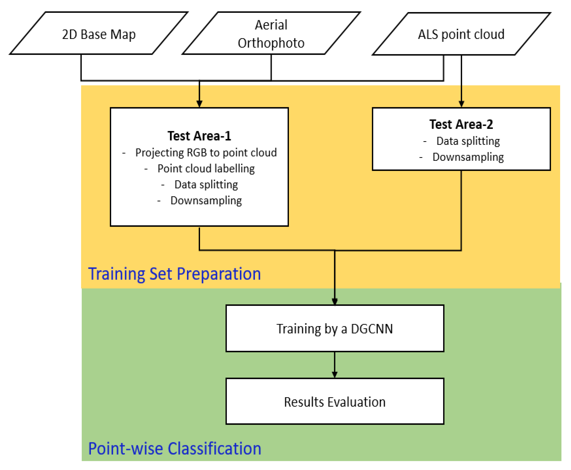
This study takes a point cloud colored by an orthophoto as an input to estimate automatically 2D urban map objects. These consist of building blocks and road networks in vector format (polygon or polyline). Our methodological workflow consists of two main tasks: training set preparation and classification and involves two different test areas (Figure 1). Point cloud classification as defined in this study refers to the task of assigning a predefined class or semantic label (e.g., bare land, building, tree, road) to each individual 3D point of a given point cloud, which is also known as semantic segmentation or class labeling.
3.1. DGCNN
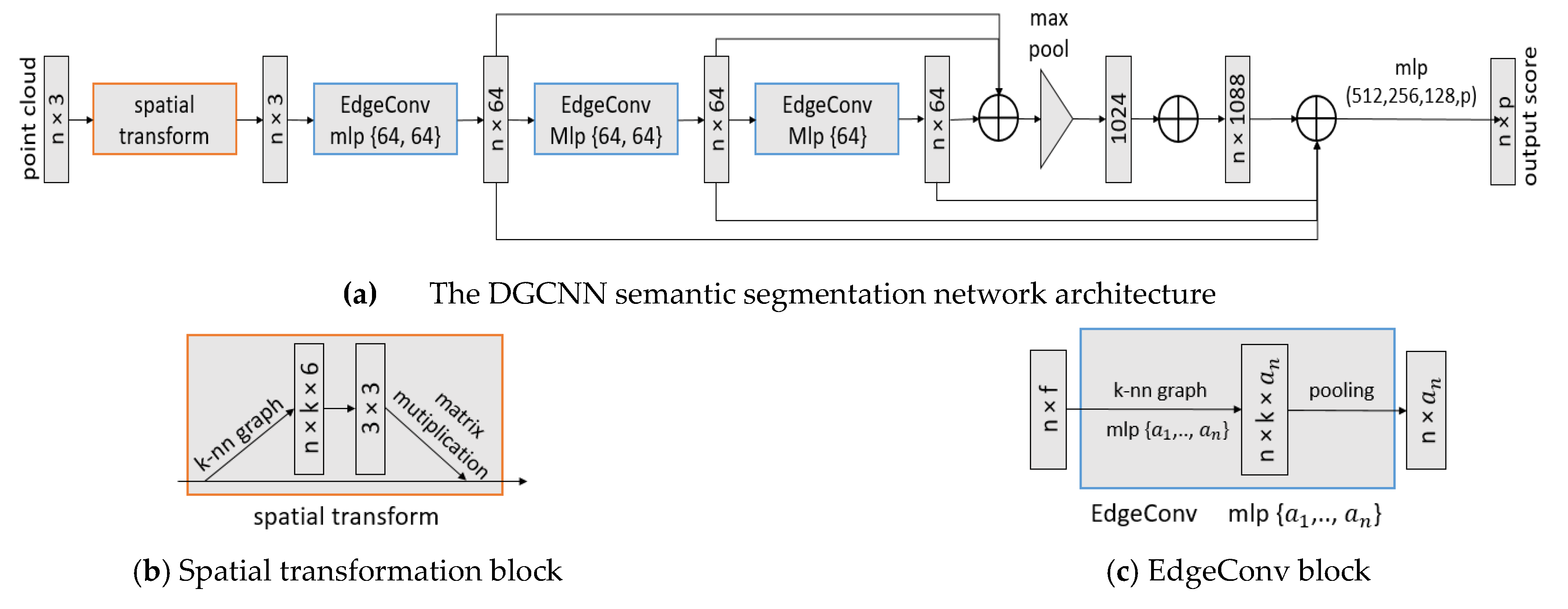
To examine different parameter settings for ALS point cloud classification, this study uses a Dynamic Graph CNN (DGCNN) architecture proposed by Wang et al. [19]. DGCNN is a point-wise neural network architecture that combines PointNet and a graph CNN approach. The network architecture uses a spatial transformation module and estimates global information, akin to PointNet. The Dynamic Graph CNN approach captures local geometric information while ensuring permutation invariance. It extracts edge features through the relationship between a central point and neighboring points by constructing a nearest-neighbor graph that is dynamically updated from layer to layer.
Based on the architecture of PointNet, the DGCNN architecture (see Figure 2) incorporates a so-called EdgeConv module to capture local geometric features from points, which is missing in previous point-wise deep learning architectures [33]. EdgeConv constructs a local graph between a point and its k-nearest neighbor points and applies convolution-line operations on the graph edges. DGCNN uses PointNet [5] as the basic architecture but combines it with graph CNNs. Instead of using fixed graphs, as other graph CNN methods do, EdgeConv updates its neighborhood graphs dynamically for each layer of the network, thereby effectively increasing the spatial coverage of the neighborhoods as the convolution step between layers downsamples the point cloud.
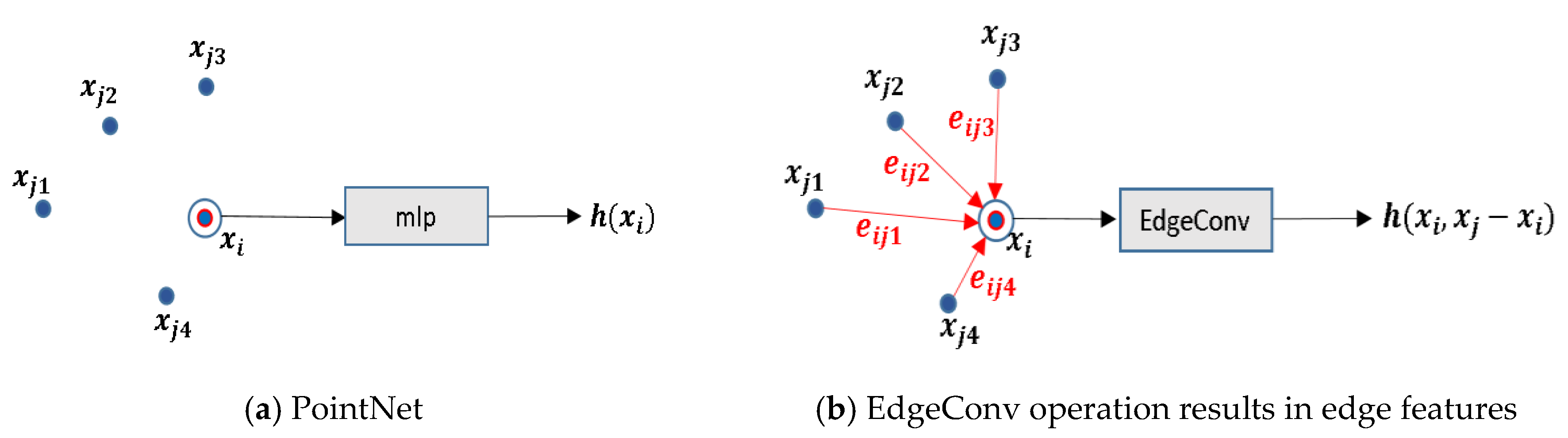
Each EdgeConv block applies an asymmetric edge function across all layers to combine both the global shape structure (by capturing the coordinates of the patch center) and the local neighborhood information (by capturing )) as shown in Figure 3. Similar to PointNet and PointNet++, the aggregation operation to downsample the input representation in DGCNN is max pooling.
To demonstrate the feasibility of DGCNN to classify huge ALS point cloud data, this study uses two study areas of different sizes, characteristics, and input point cloud specifications. Area-1 (city of Surabaya, Indonesia) represents a metropolitan urban area dominated by dense settlements while Area-2 (city of Utrecht, the Netherlands) has more variation in urban land use. Datasets of both study areas exhibit imbalances in their class distribution. Area-1 has a total size of 5 km2 while Area-2 has a total size of 25 km2.
3.2. Area-1
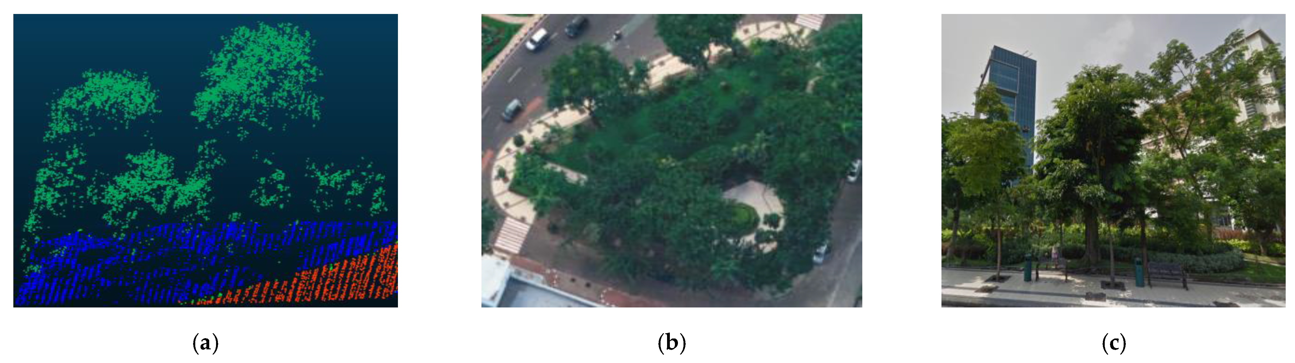
The first test area is located in the second-largest Indonesian metropolitan area, Surabaya city in West Java Province. The city is characterized by dense settlement areas with various types of well-connected roads. Surabaya city is home to numerous high-rise buildings and skyscrapers. Many parks exist and vegetation in Surabaya city is dominated by trees (see Figure 4). For this study area, we classify the 3D point cloud into four classes: bare land, trees, buildings, and roads. Due to the limited number of LiDAR points covering water in the study area, a water class is not included.
Area-1 covers 21.5 km2 and consists of 354.2 million points. The ALS point cloud was captured by an Optech Orion H300 instrument and has an average density of about 30 points/m2. The aerial photos captured at the same time by a tandem camera have spatial resolutions of 8 cm with less than 15 cm positional accuracy. The ALS point cloud is divided into two classes: ground and nonground points. The dataset was projected in the UTM49 South coordinate system using the WGS84 geoid. Both LiDAR point cloud and aerial photos were acquired from the same platform at the same time in 2016. The reference data used to label the points and to evaluate the final results are an Indonesian 1:1000 base map from 2017. The base map was acquired by manual 3D delineation from the same aerial photos.
3.2.1. Training Set Preparation
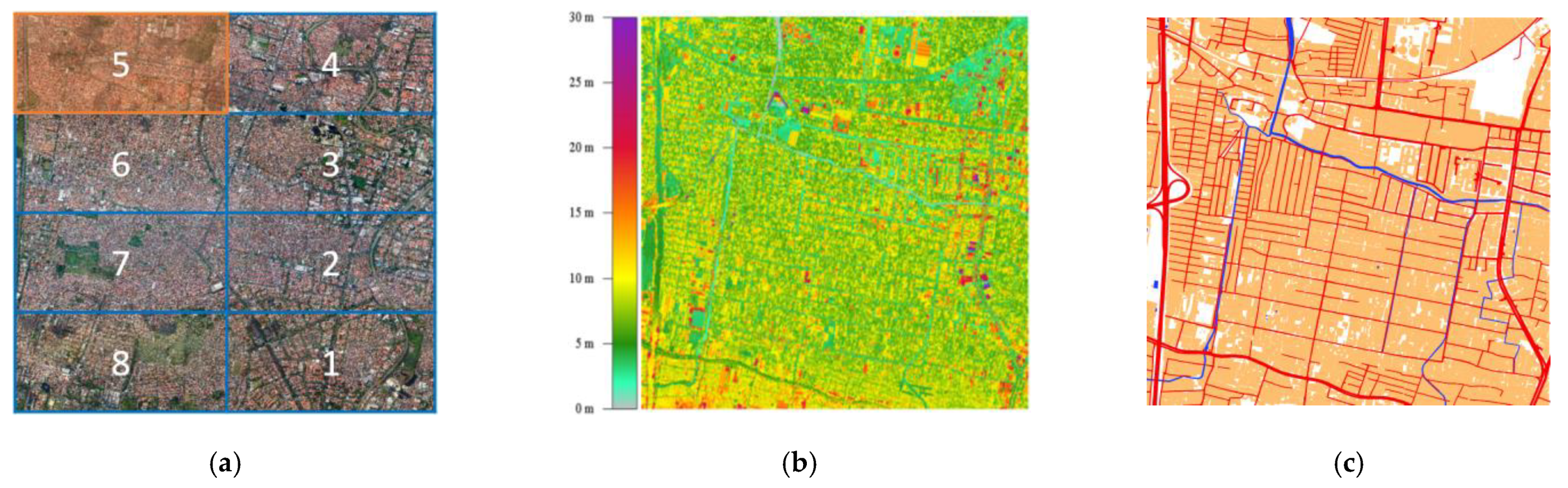
To efficiently process the points, the 3D point cloud of Area-1 is divided into 8 grids (see Figure 5a) and each grid is split into 16 tiles. Tile no. 5, located in the top left part of Area-1, is used as a test area and remaining tiles are used for training.
In preparing the training set, we first projected RGB (Red, Green, Blue) color information from an orthophoto onto the ALS point cloud data by nearest neighbor. Next, the point cloud data were downsampled to 1 m 3D spacing for efficiency and to facilitate the capturing of global information.
To label the training data, 2D building and road polygons from the 1:1000 base map of Surabaya city were used. Although the point cloud data used in this study were already classified into ground and nonground points, two challenges needed to be solved when the 2D base map was used to label the point cloud. First, the corresponding base map does not provide information on trees. Second, as we use 2D base map polygons to label the points, the labeled building and road points may include many mislabeled points in cases where trees exist above buildings or roads. Therefore, we performed hierarchical filtering to label tree and bare land points based on surface roughness. The method is also intended to improve the quality of the training samples by removing likely mislabeled points on buildings and road points.
The labeling criteria are as follows:
- nonground points are labeled as buildings using 2D building polygons of the base map. Using the same method, ground points were labeled as road. Remaining points were labeled as bare land;
- from the points labeled as building or road, any point that has surface roughness above a threshold is relabeled as tree. The surface roughness was estimated for each point based on the distances to the best fitting plane estimated using all neighboring points inside an area of 2 m 2 m. Given the resulting roughness values for both trees and building points in selected test areas, and given the fact that tree canopies in the study area have minimum diameters of about 3m, the roughness threshold was set to 0.5 m;
- a Statistical Outlier Removal (SOR) algorithm was performed to remove remaining outliers. We set the threshold for the average distance () = 30 and multiplier of standard deviation = 2. This means that the algorithm calculates the average distance of 30 k-neighboring points and then removes any point having distance more than ;
- as the final step, training samples data were converted to the hdf5 (.h5) format by splitting each part of the area into blocks of size 30 30 m with a stride of 15 m. Based on our experiments in Area-1, these parameter values give the best accuracy. However, to ensure that the network uses an efficient spatial range, the block size may require an adjustment if applied to study areas of different characteristics.
3.2.2. The Choice of Feature Combinations and Loss Functions
Similar to PointNet and DGCNN, each point in the point cloud input was attributed to a nine-dimensional feature vector consisting of three spatial coordinates () and six additional features. Candidate additional features are: spectral color information (Red, Green, Blue), normalized 3D coordinates , and off-the-shelf LiDAR features (intensity, return number, and number of returns). Normalized 3D coordinates are used as additional features by PointNet, PointNet++, DGCNN, and other networks to boost the translational invariance of the algorithm (Qi et al. 2018). Normalized 3D coordinates, in which the point cloud original coordinates are transformed to a common space coordinate (ranging from 0 to 1) by subtracting values by its central 3D coordinates of each tile, are expected to give global information. In the indoor case, normalized point coordinates provide a strong indication on the type of object (e.g., floors always have Z values close to 0, walls have X or Y values at 0 or 1, etc.). This study tries to investigate the effectiveness of such normalized coordinates in the outdoor scenarios of orthogonal airborne point clouds. To evaluate the contribution of each feature, we compare four different sets of feature vectors as presented in Table 1.
Combinations of different input features are explained as follows:
- Feature Set 1 uses the default feature combination, as widely used by indoor point cloud benchmarks (e.g., S3DIS dataset).
- Feature Set 2 replaces RGB color with LiDAR features (Intensity, Return number, and Number of returns (IRnN)) to evaluate the importance of LiDAR features.
- Feature Set 3 combines two color channels (Red and Green) with LiDAR intensity to investigate the importance of spectral features.
- Feature Set 4 combines full RGB color features and LiDAR IRnN features and excludes normalized coordinates to evaluate the importance of global geometry.
Deep neural networks learn to map inputs to outputs based on the training data. At each training step, the network compares the model predictions to actual labels to determine and increase the model performance. Typically, gradient descent is used as optimization algorithm to minimize errors and update the current model parameters (weights and biases). To calculate the model error, a loss function was used.
A class imbalance exists in Area-1 because it is heavily dominated by buildings (59%) and trees (19%). Therefore, we investigated two different loss functions that are incorporated within the DGCNN architecture: softmax cross entropy loss and focal loss [31].
- Softmax Cross Entropy (SCE) loss. This is a combination of a softmax activation function and cross entropy loss. Softmax is frequently appended to the last fully connected layer of a classification network. Softmax converts logits, the raw score output by the last layer of the neural network, into probabilities in the range 0 to 1. The function converts the logits into probabilities by taking the exponents of the given input value and the sum of exponentials of all values in the input. The ratio between the exponential input value and the sum of exponential values is the output of softmax. Cross entropy describes the loss between two probability distributions. It measures the similarity of the predictions to the actual labels of the training samples.Consider a training dataset with input points within a batch of size , and is the -th label target class (one-hot vector) among . denotes the feature vector before the last fully connected layer of classes. and , represent the trainable weights and biases of the -th class in softmax regression, respectively. Then the SCE loss is written as follows:
- Focal loss is introduced to address accuracy issues due to class imbalance for one-stage object detection. Focal loss is a cross entropy loss that weighs the contribution of each sample to the loss based on the classification error. The idea is that, if a sample is already classified correctly by the network, its contribution to the loss decreases. Lin et al. [31] claim that this strategy solves the problem of class imbalance by making the loss implicitly focus on problematic classes. Moreover, the algorithm weights the contribution of each class to the loss in a more explicit way using Sigmoid activation. The focal loss function for multiclassification is defined as:where denotes the number of classes; equals 1 if the ground-truth belongs to the -th class and 0 otherwise; is the predicted probability for the -th class; is a focusing parameter; is a weighting parameter for the -th class. The loss is similar to categorical cross entropy, and they would be equivalent if and
3.2.3. Training Settings
During training, 4096 points are uniformly sampled from each training block of size 30 30 m, Section 4.1, to form data batches with a consistent number of points, while all points are used during testing. This study uses nine features for training; therefore, the size of the data fed into the network is . We used nearest neighbors for each point to construct the k-nearest neighbor graph. For all experiments, the final model was obtained after running 51 epochs, optimized by an Adam optimizer with an initial learning rate of 0.001, a momentum of 0.9, and a mini batch size of 16. The 3D point cloud semantic segmentation using DGCNN was performed in the High-Performance Computing (HPC) environment of Delft University of Technology, consisting of 26 computing nodes. For training, two Tesla P100-16GB GPUs were used.
3.3. Area-2
Area-2 uses open source point cloud data of the Dutch up-to-date Elevation Archive File, version 3 (AHN3) downloaded from PDOK [34] and a ready-made geodata webservice [35]. Each individual 3D point came labeled as one of the following classes: bare land, buildings, water, bridges, and others. The “others” class consists mostly of trees and other vegetation, but also includes objects such as railways and cars. Since points classified as bridges are sparse, in this study, bridge points were merged into the bare land class.
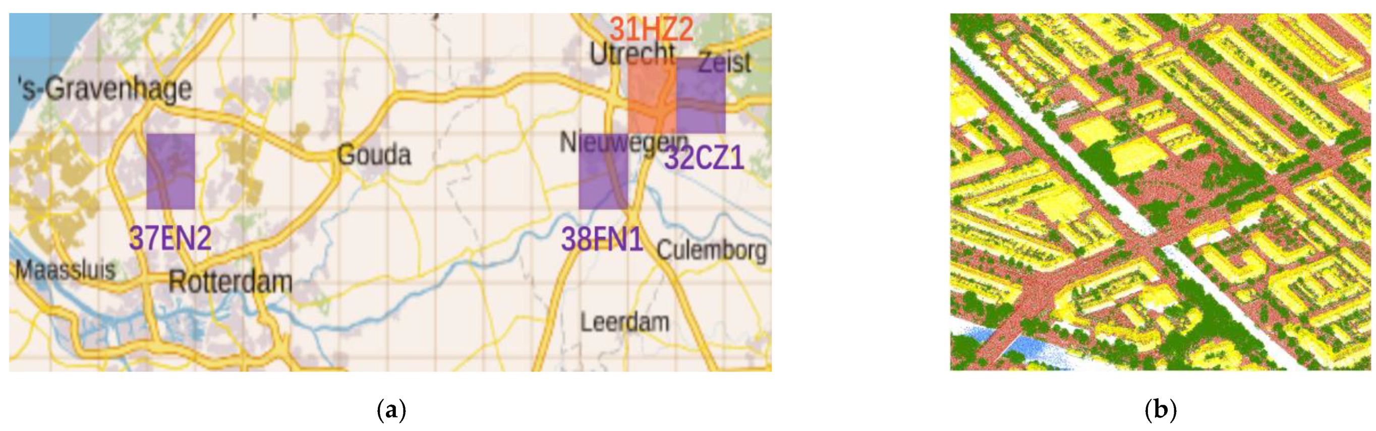
This study uses the same AHN3 point cloud dataset used by Soilán et al. [20]. The dataset consists of four grids of AHN3 point clouds located in the surroundings of the city of Utrecht and Delft (see Figure 6) with a total number of about 190.3 million points. Each grid has an area of 6.25 5 km2 and a unique ID. The original dataset has an average point density of 20 points/m2.
If a deep learning method such as DGCNN would be successful in classifying AHN3 data based on available AHN3 labels for different areas, this opens new possibilities for cheaply labeling future version of AHN. Thus, AHN4 or AHN5 could be automatically classified using available class labels from previous editions.
3.3.1. Training Set Preparation
Each grid of the AHN3 point cloud was split into 25 tiles and downsampled uniformly with a point interval of 1 m. In total, 12 tiles from 38FN1, 37EN2 and 31HZ2 were used and only eight tiles from 32CN1 were used since this grid contains a large amount of vegetation, which leads to more points due to multiple returns. The number of used points is summarized in Table 2.
Apart from x, y and z coordinates, all points from AHN3 are also provided with extra attributes, such as return number, intensity, GPS time, etc. For Area-2, nine features were used, including 3D coordinates (x, y, z), LiDAR features (return number, number of returns, and intensity), and normalized coordinates (nx, ny, and nz). Classification of AHN3 point clouds by the DGCNN architecture was implemented in the PyTorch framework [36].
3.3.2. The Choice of Block Size
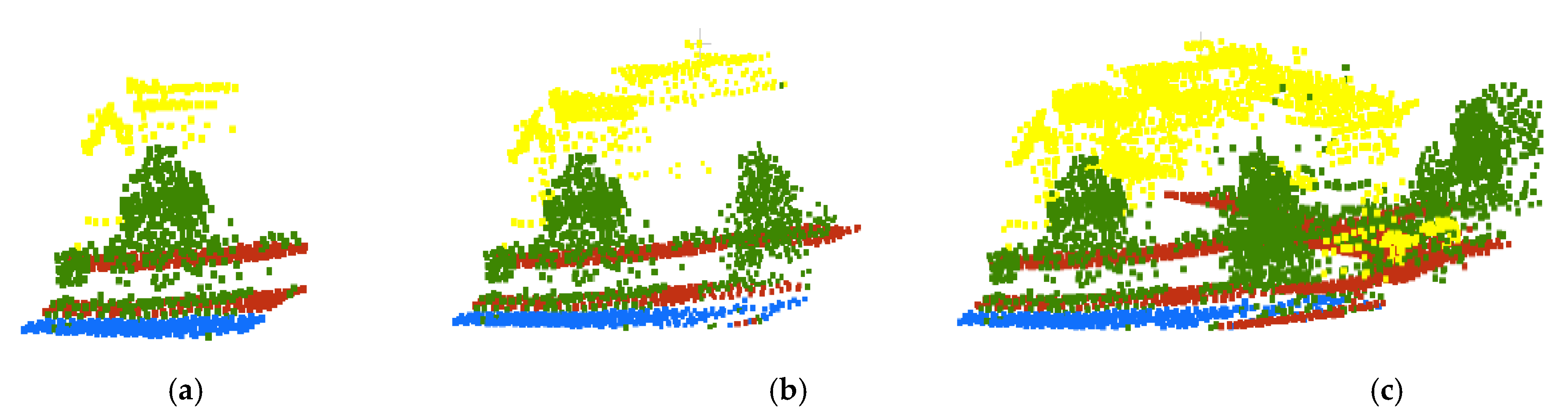
For DGCNN, a point cloud needs to be split into 3D blocks with a certain block size (see Figure 7). In training mode, points with point features, are randomly sampled from a single block and put into the neural network. In DGCNN, the -nn graph is dynamically updated in feature space from layer to layer. Thus, it is difficult to compute the effective range using a simple equation. What we know for sure is that the effective range is limited by the block size and affected by the size of the neighborhood of each point as defined in the -nn graphs. Based on our test on different -values, gives the best result.
To investigate the feasibility of DGCNN for classification of aerial point clouds and the influence of different effective ranges, using the determined -value (), we experimented with three different block sizes: 30, 50 and 70 m (Figure 7).
3.3.3. Training Settings
For the Area-2 experiment, 4096 points were randomly sampled from each block during training before being fed into the neural network. To ensure some overlap between different blocks, we used 1.5 as the sample rate for each point. This means that to determine the number of blocks, the total number of points in the point cloud will be multiplied by a sample rate of 1.5 and then divided by 4096. In the test stage, the sample rate was set as 1.0 and all points in each block were used. During training, the batch size was 8, which meant eight blocks could be processed at the same time. However, we used a batch size of only 1 during testing, since the number of points was different in each block when no random sampling was used and different blocks cannot be stacked together. The network was optimized by an Adam optimizer with an initial learning rate of 0.001, as suggested as the default in DGCNN [18]. For all experiments, the model used in testing was obtained by choosing the best model after training with 50 epochs. For Area-2, one NVIDIA GeoForce RTX 2080 Ti GPU was used.
3.4. Evaluation Metrics
Given the complexity of digital classification, selecting reliable quality metrics to assess the classification results is crucial [37]. For assessing the classification results, this study used evaluation metrics that are mainly used in deep learning and remote sensing classification research [38,39,40]. This study used different feature combinations, loss functions, and block sizes for the point cloud classification. Several selected quality metrics are described as follows:
- Overall accuracy, indicating the percentage of correctly classified points of all classes from the total number of reference points. This metric shows general performance of the model, and thus may provide limited information in case of class imbalance.
- The confusion matrix is a summary table reporting the number of true positives, true negatives, false negatives, and false positives of each class. The matrix provides information on the prediction metrics per class and the types of errors made by the classification model.
- Precision, recall, and F1 score: Precision and recall are metrics commonly used for evaluating classification performance in information technology and are related to the false and true positive rates [41,42]. Recall (also known as completeness) refers to the percentage of the total points correctly predicted by the model, while the precision (also known as correctness) refers to the percentage of correctly classified points in all positive predictions. The F1 score is a weighted average of precision and recall to measure model accuracy. The metrics are formulated as follows:
4. Results and Discussions
4.1. Area-1
For ALS point cloud classification in Area-1, four different feature combinations and two loss functions were compared. The total number of samples used for training was 30.929.919 points, dominated by building points (59%). Trees, bare land, and road classes are sampled by 21%, 13% and 7%, at the points, respectively.
4.1.1. Results of Different Feature Combinations
To investigate the best feature combination to classify ALS point cloud colored by an orthophoto using a deep learning approach, three different metrics (completeness/recall, correctness/precision, and F1 score) along with Overall Accuracy (OA) were used. Some results are visualized in Figure 7. Table 3 shows the classification results of all predefined feature combinations and loss functions used in this study. Based on the evaluation results, Feature Set 4 achieved the highest overall accuracy (91.8%) and F1 score for all classes.
In general, the use of normalized coordinate features in combination with other features is not as effective as the combination of spectral color with LiDAR features. The use of full RGB color and off-the-shelf LiDAR features significantly improves the F1 score of trees by at least 7% and buildings by 5.7%.
Based on the class quality metrics presented in Table 4, the potential of different feature combinations to predict different land cover classes in our test area is discussed below:
- Bare land class
The lowest recall rate was achieved by Feature Set 4. This indicates that normalized 3D coordinates are useful to detect bare land correctly. The highest recall rates are achieved by Feature Set 4. This is because Feature Set 4 produces fewer False Positives (FPs), which makes the precision rate higher. A combination of LiDAR intensity and normalized coordinates (Sets 2 and 3) effectively maintains a high number of points correctly classified as bare land, indicated by high recall (92.1%). On average, the road class considerably had the lowest recall rates while the bare land class always had the lowest precision. This indicates that there is high confusion between bare land and roads, which we assume mainly happens due to the presence of open areas having similar heights and the same color such as parking areas, front yards, and backyards.
- Tree class
Feature Set 4 obtains the highest recall and precision rates with scores of 84.3% and 93.3%, respectively. The use of both RGB color and LiDAR information in Feature Set 4 significantly increased the tree detection by almost 11% compared to the other feature sets. In general, the main source of error was trees misclassified as buildings, which particularly occurs for trees adjacent to buildings. Our results also show that there are more trees misclassified as buildings than buildings detected as trees which results in recall rates that are always lower than precision.
- Buildings
The recall and precision rate of building detection remarkably improved when using Feature Set 4. It is likely that the decreasing number of confusions between buildings and trees induces higher building classification accuracy. One of the biggest error sources for building classification are small details on roofs and building façades that are classified as trees.
- Roads
Although the road detection accuracy is not as good as other classes, the highest recall and precision rates were achieved by Feature Set 4 with scores of 81.6% and 86.9%, respectively. Using RGB and intensity (Set 4) as input features significantly improved the recall rate of roads by reducing the number of road points detected as bare land. As our study focuses on urban classification and base map generation, points on cars or trucks were labeled as roads. Given the results, the road classification results were not very much affected by the presence of cars.
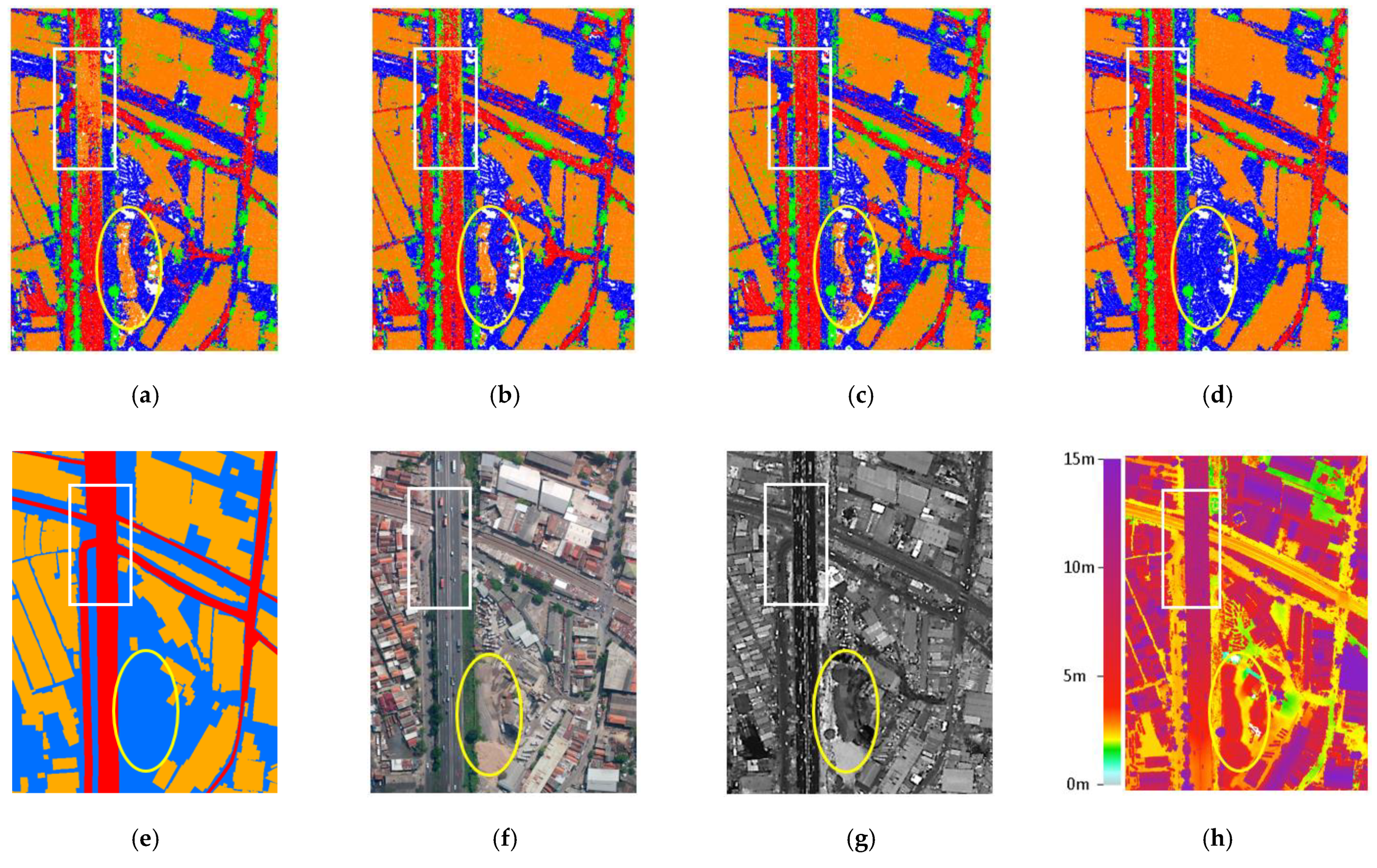
Figure 8 visualizes the classification results of different feature combinations over a subset of our test area in comparison to the following data sources: base map, orthophoto, LiDAR intensity, and digital surface model (DSM). The white rectangle highlights an area where most classification results fail to detect a highway and an adjacent road of different heights. Feature Set 1 resulted in a misclassification of some points on the overpass highways as buildings and the adjacent road below the highway were falsely classified as bare land (white rectangle in Figure 8a). Because road, buildings, and bare land have similar geometric characteristics (e.g., planarity), using the LiDAR intensity feature in addition is beneficial to increase the road classification accuracy.
A sand pile existed in the study area due to construction work at the time of data acquisition (yellow ellipses in Figure 8). Only Feature Set 4 correctly classified the sand pile points as bare land while other feature sets falsely classified points on the sand pile as buildings. This suggests that using complementary airborne LiDAR and spectral orthophoto features increases detection accuracy.
4.1.2. Results of Different Loss Functions
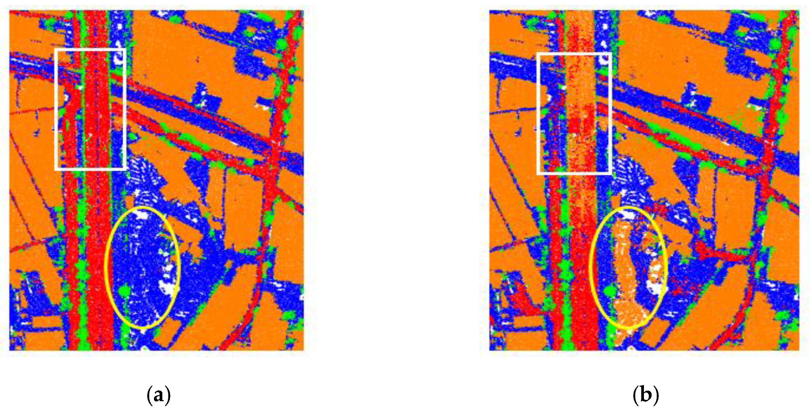
Even though class imbalance exists in our study area, the overall accuracy was not necessarily increased by applying a focal loss (FL) function as may be expected. Table 5 shows the results of Feature Set 4 when using two different loss functions: SCE and FL ( = 0.2, γ = 2). The overall accuracy (OA) of the results of Feature Set 4 decreased by 3.7% when FL was used. However, the F-1 score for the bare land and road classes dropped by ~6% and ~15%, respectively, when FL was used. Our explanation for this is that the loss function focuses on decreasing the loss of the classes that produce large amounts of misclassified points, in this case buildings and trees, thereby somehow neglecting bare land and, notably, roads.
Based on the confusion matrix presented in Table 6, Feature Set 4 in combination with FL has the highest precision rate (86.7%) for trees, but the number of correctly detected tree points is lower than for the other feature sets. This is because FL focuses on increasing the detection rate by evaluating the errors of the dominant class so that the number of misclassified tree points decreases. For building classification, the highest recall (93.7%) was achieved when using FL with only 0.3% recall difference to the results obtained by SCE. For road classification, the use of FL doubled the number of false negatives compared to SCE.
The white rectangles and yellow ellipses in Figure 9 indicate (a) an area where some parts of the highway were misclassified as buildings and (b) a sand pile that was misclassified as a building when using focal loss (FL). For our purposes, the SCE loss function performed better then FL in the DGCNN architecture.
4.1.3. Results on Area with Relief Displacement
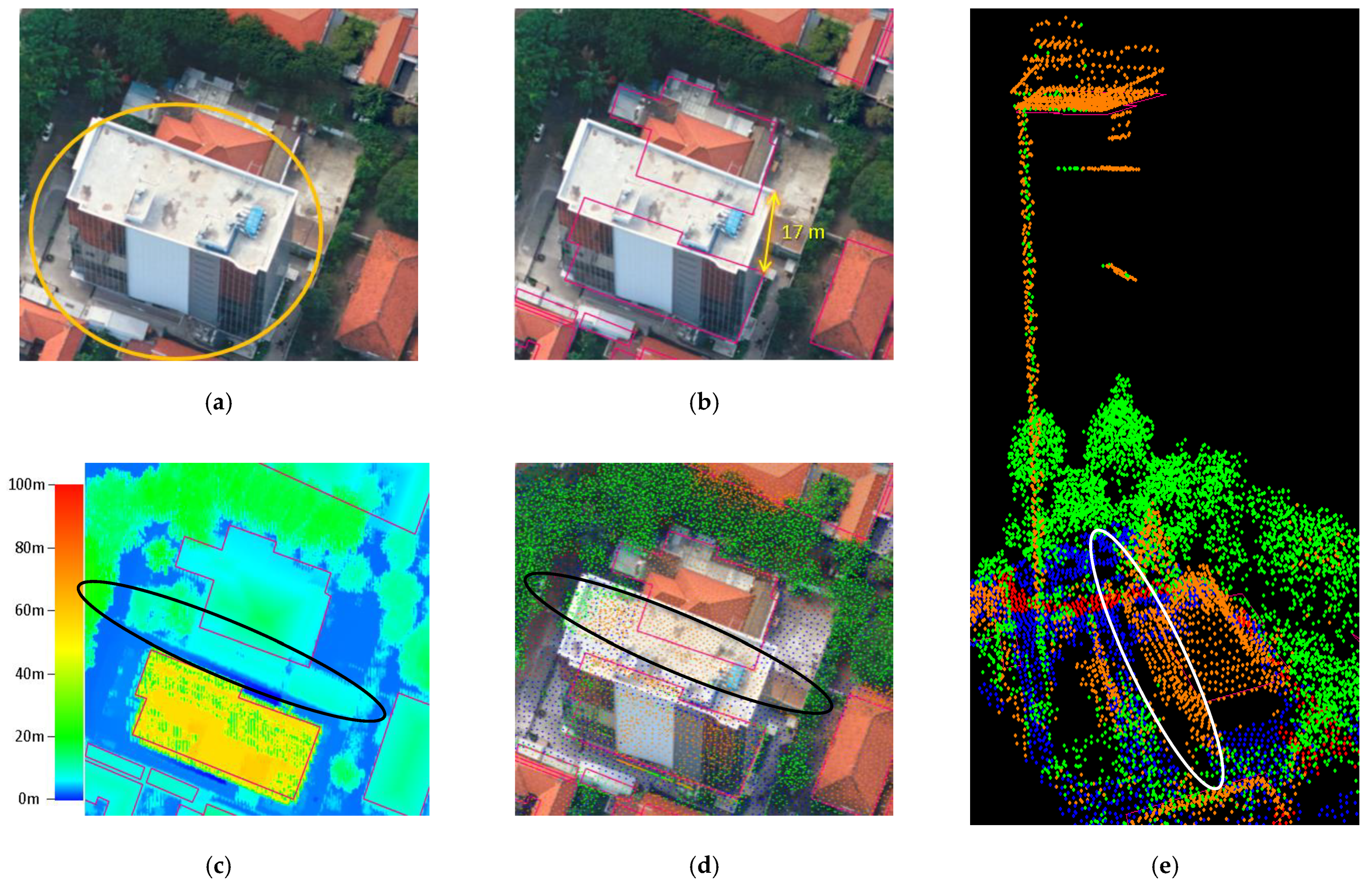
One drawback of using aerial photos is the positional shift of highly elevated objects (e.g., high-rise buildings). This effect is called relief displacement and is caused by variations in the camera angle. Displacement errors increase with the height of the object and the distance to the acquisition location. Objects suffering from relief displacement in photos usually have bigger sizes in the photo than in reality, as some parts of vertical walls are exposed and buildings appear to lean in one specific direction. In aerial photo classification, relief displacement is considered as one of the main sources of mislabeling (Chen et al., 2018). Figure 10 shows a relief displacement error in an orthophoto of a leaning building that blocks a lower building and nearby trees.
ALS point clouds can be used to detect objects blocked by high-rise buildings that even a human operator cannot identify in an orthophoto. For example, part of a building in Figure 10c (highlighted by a white ellipse) was automatically and correctly detected by our method (yellow outline) but is missing in the building reference (pink outline). This means that even though we used ground orthophotos to color the point clouds, which, as a consequence, resulted in wrongly colored points in case of relief displacement, the network we employed still classified the points correctly. It is likely that, during training, DGCNN is able to learn and give smaller weights or big penalties to the color features in case relief displacement exists, thereby favoring the geometric point cloud information.
4.2. Area-2
With a total of 109,389,471 points, Area-2 is dominated by the “others” class (57.6%). The ground and building classes occupy percentages of 30.9% and 11.9%, respectively. Water has the smallest representation with a percentage of 0.6%. Table 7 summarizes the quantitative results of point cloud semantic segmentation over Area-2 for different block sizes and a fixed neighborhood size of . The best overall accuracy (93.28%) and average F1 score were achieved with a block size of 50 m. Block size of 30 m had the lowest overall accuracy (91.7%) and per class F1 score, indicating that, in Area-2, more balanced results among different classes can be obtained when the block size is larger.
Considering the recall and precision values shown in Table 8, points from the “other” and ground classes were identified well in all block sizes with high values in both recall and precision. This is not surprising considering the high number of points in both classes compared to other categories. When the network processes point clouds of bigger blocks, the predicted building points have better recall but lower precision rates which means the model misses a certain number of building points, although most predictions are correct. For the water class, when the block size is very large (70 m), the precision is worse than recall rate, indicating that the model is not accurate enough for detecting water points. Compared to the other classes, the water class always has the lowest precision and recall rates. This is because the number of points on water in our Area-2 is much less than other classes.
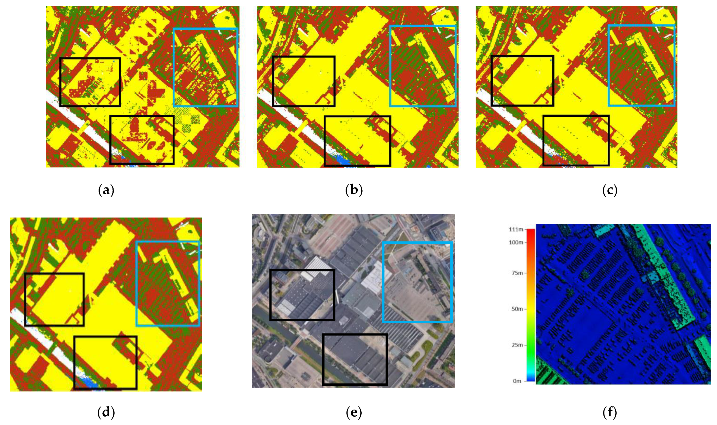
Figure 11 illustrates the point cloud classification results for different block sizes. Points on big buildings are often classified as bare land for a block size of 30 m (see black rectangles). This is likely because, in some areas with large building roofs, the block only contains building points. As points on both building roofs and bare land share similar characteristics, a block mainly containing building points is falsely classified as bare land. In this subarea, a block size of 30 or 70 m classifies most of water points as bare land, while using a block size of 50 m results in a correct classification of most water points.
As indicated by the blue box, a large number of points from the “other” class (in this case parked cars) are labeled as buildings when the block size is 30 m. This happens, presumably, because the points on cars and buildings both have planar surfaces at different height. With a bigger block size, most of points on parked cars are correctly classified as “others”. In this case, a bigger block size sufficiently provides an effective spatial range to the network for recognizing the differences between buildings and cars.
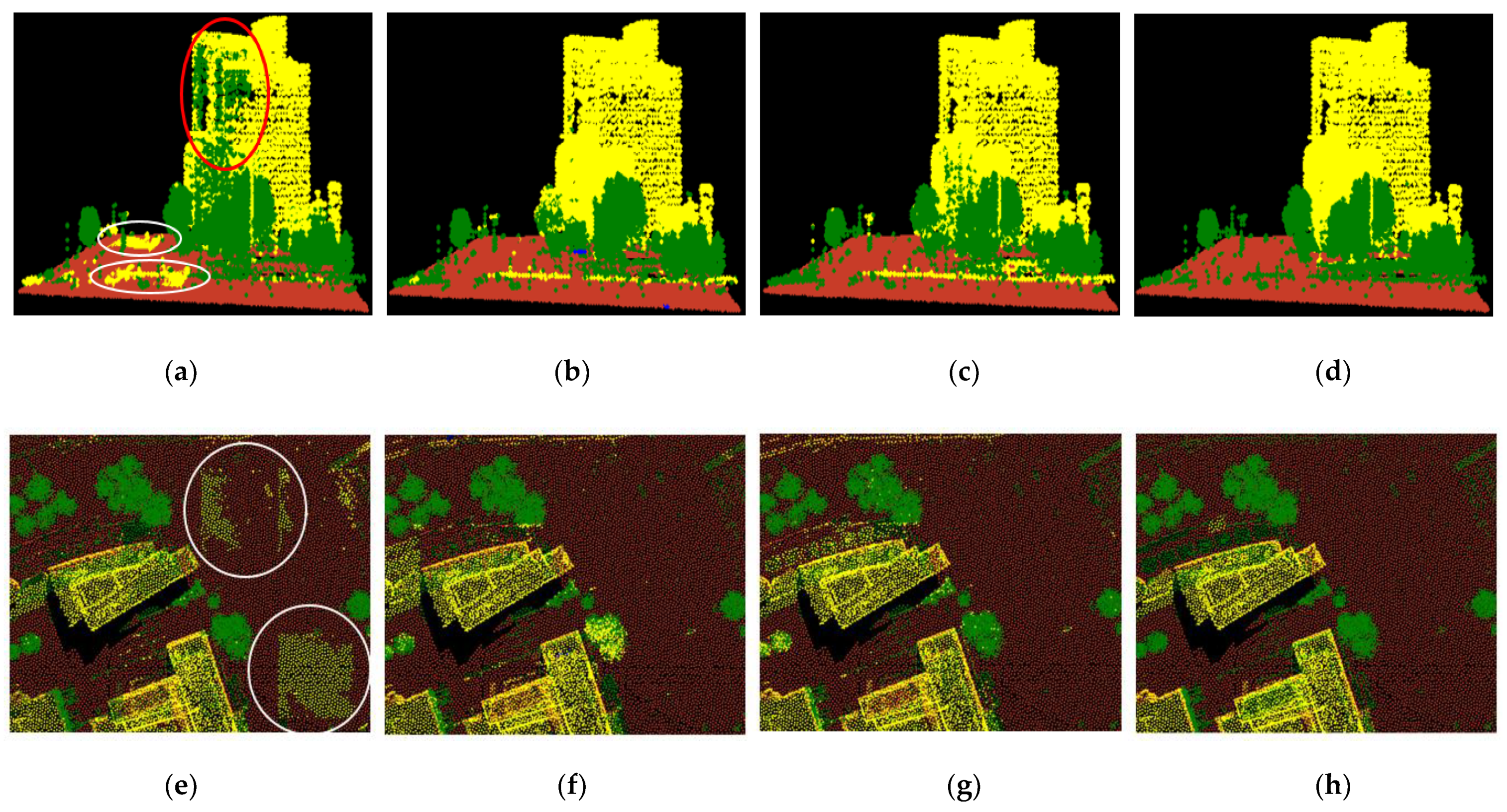
Other examples in Figure 12a,e, respectively, show 3D and 2D visualizations of classification results when using a block size of 30 m. Some points on building façades are labeled as “others” (see red ellipse). There is also a “block effect” highlighted by the white ellipses, where the edges of some blocks can be clearly seen. The “block effect” no longer exists and fewer points on building façades are classified as “others” when using block sizes of 50 and 70 m.
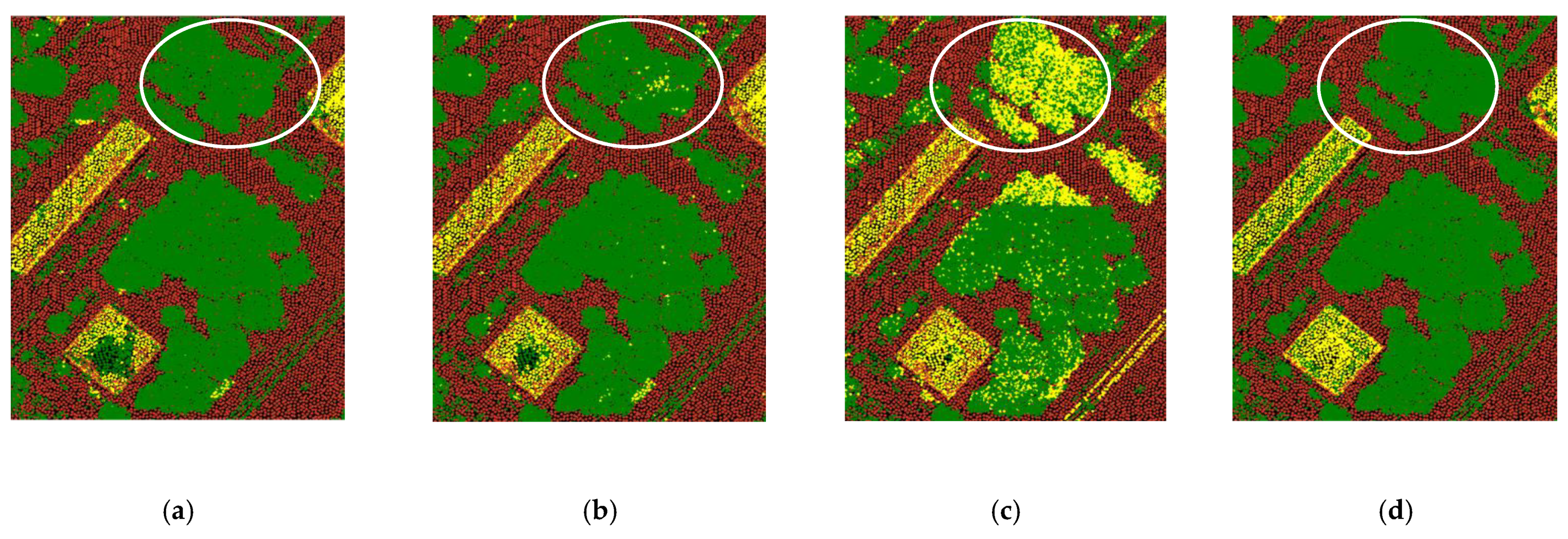
Using a larger block size, however, does not always result in better classification accuracy. Based on our results, more “others” points, typically tree points, were misclassified as buildings when using bigger block sizes. As shown in Figure 13, a block size of 30 m classifies “others” (tree) points best, while a block size of 70 m has the highest misclassification rate on “others” (trees)—see white circles. A possible explanation is that a larger block size will result in lower point density that later causes some key points and details to be missing—e.g., tree canopies may appear more flat which makes them resemble building roofs to some extent. This suggests that the network requires a higher point density to capture the essential characteristics of trees. Thus, selecting the optimal block size for point cloud classification should be carefully determined because there is an accuracy tradeoff between different object classes—in our case, this is between trees and buildings.
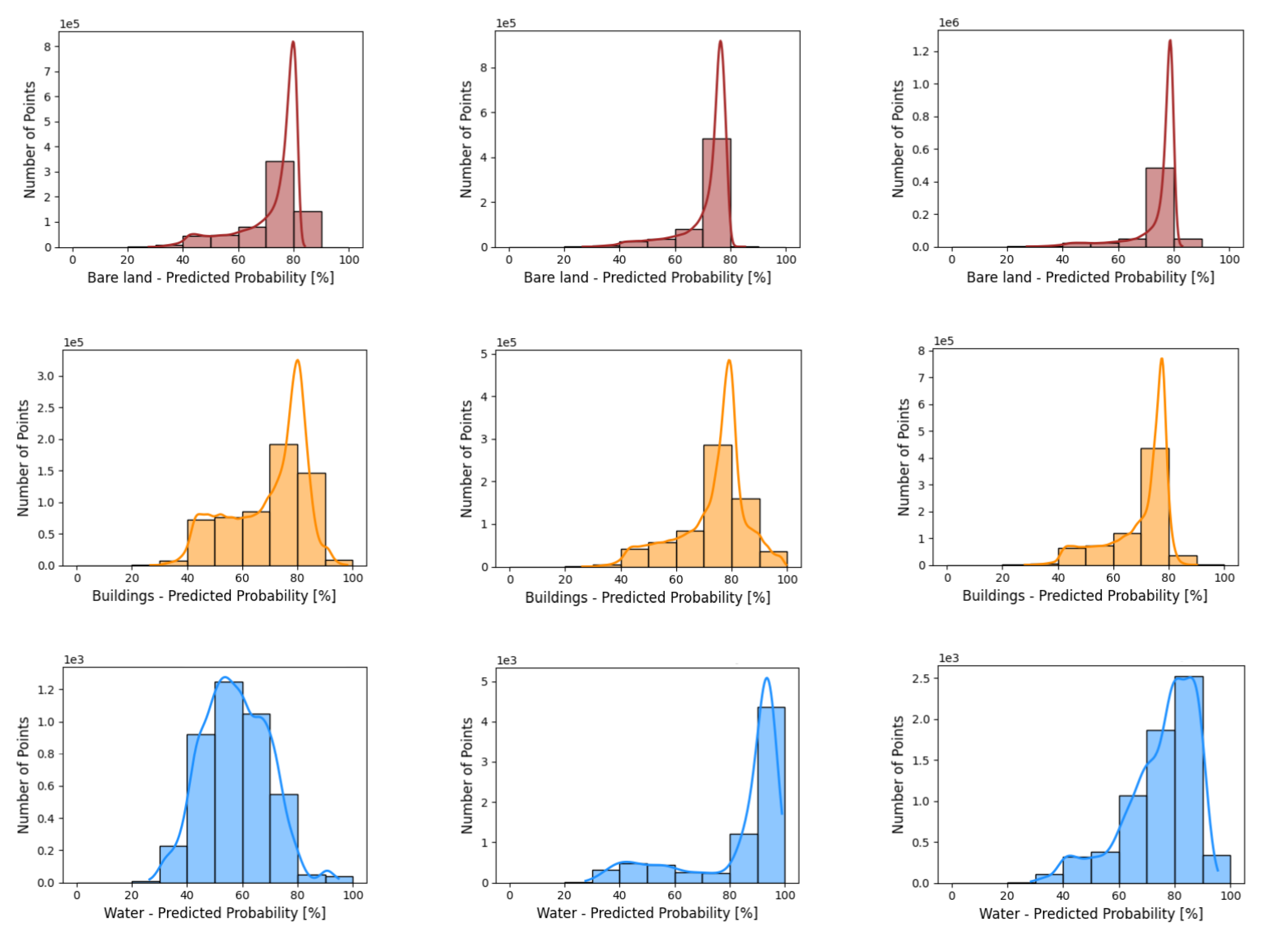
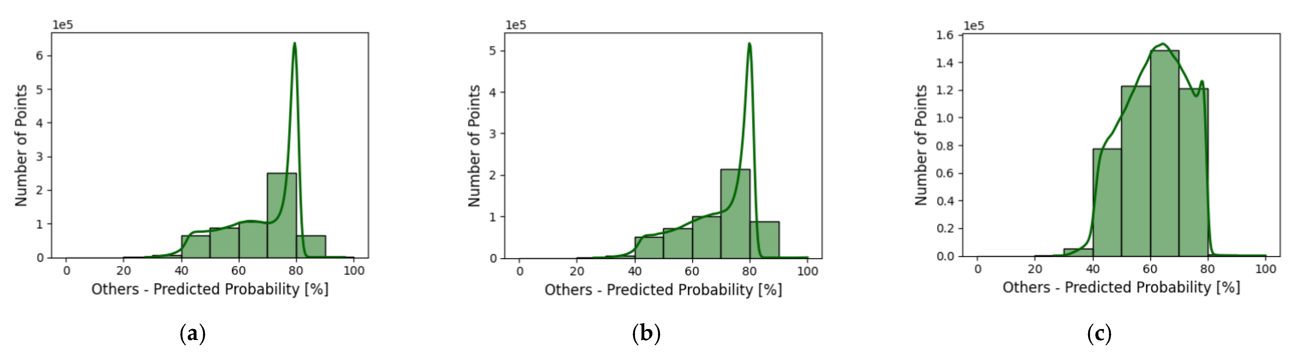
As an additional evaluation, this study provides per class probability distributions over the test dataset as obtained by the network with different block sizes—see Figure 14. The histograms contain the confidence level of the models in predicting the “winning” classes. In general, the histograms are consistent with the F1 score results presented in Table 7.
The model has high confidence when predicting bare land using any block sizes as most of the bare land points have more than 80% confidence. The building class shows a wider range of confidence level ranging between 40% and 80%. The building class with a block size of 30 m has more points with a lower confidence result (below 70%). Apparently, this proves that using a smaller block size may result in lower building accuracy.
Compared to other classes, the histograms for water and “others” classes have significant differences when using different block sizes. The water class has the lowest confidence (40–60%) when using a block size of 30 m and has the highest confidence level when using a block size of 50 m (above 90%). When using a block size of 70 m, water class has the second best confidence level ranging between 75% and 90%. Considering that the water class has the smallest point representation, using an appropriate block size can eliminate the influence of class imbalance.
The confidence level when predicting the probability of the “others” class is high (around 80%) when using both block sizes of 30 and 50 m. However, when predicting the “others” class with a block size of 70 m, the model confidence drops to values between 50% and 80%. This is consistent with our findings that using a bigger block size results in lower tree classification accuracy.
5. Conclusions and Recommendations
This study investigated the feasibility of DGCNN for ALS point cloud classification over urban areas and discusses how different settings of input feature combinations, loss function, and block size affects classification results. Several experiments on two different areas indicate that using DGCNN with proper settings is able to provide accurate results close to production requirements in classifying airborne point clouds. In Area-1, ALS point clouds colored by orthophotos were used to investigate different input feature combinations and loss functions. We labeled the training samples used for classification using the best available public vector data from a 1:1000 base map. Based on the classification results, the combination of full RGB image features and airborne LiDAR features outperforms other feature sets and significantly increases the classification accuracy by 6%. The softmax cross entropy loss function performed better than focal loss, although the latter loss function was included in the testing because of some class imbalance in our input data.
In Area-2, training samples were labeled using available class labels from the Dutch AHN distribution. We tested three different block sizes (30, 50, and 70 m) of AHN3 point clouds using LiDAR off-the-shelf input features (X, Y, Z, intensity, return number, and number of returns). A block size of 50 m provided the highest classification accuracy result (93.3%) and efficiently reduced the misclassification of building points as bare land. Moreover, balanced and good F1 scores for all kinds of objects were obtained when using a block size of 50 m. There was a trade-off between building and tree (class “others”) classification accuracy results when increasing the block size. This implies that, to classify outdoor point clouds using DGCNN or other PointNet-based deep learning architectures, block size is a crucial parameter to be carefully tuned.
In our experiments, Area-2 (91–93%) achieved a higher classification accuracy than Area-1 (83.9%) when using LiDAR input features. This could be related to the number of training samples that we used for Area-2 which is two times bigger than for Area-1.
Further research should include the development of an optimal input feature and block size selection procedures. Such a procedure should largely replace the current empirical for increasing deep learning classification accuracy. Our research indicates that 3D deep learning matured so much that it is now actually able to extract geometric information as required for digital maps or digital point cloud repositories at near-operational quality, but in a much shorter time than traditional workflows. Comparisons to other machine learning approaches, which also include computational costs, would be interesting to study. Furthermore, the applicability of our method to data representing other cities and countries as well as possible extensions to rural environments is a beneficial direction for future research.
Author Contributions
E.W. designed the workflow and responsible for the main structure and writing of the paper. E.W., Q.B. and M.K.F. conducted the experiments and discussed the results described in the paper. R.C.L. gave comments and editions to paper writing. All authors have read and agreed to the published version of the manuscript.
Funding
This research was financially supported by the Indonesia Endowment Fund for Education (LPDP) as a part of PhD research conducted under the Department of Geoscience and Remote Sensing of TU Delft and the APC was funded by Delft University of Technology.
Institutional Review Board Statement
Not applicable.
Informed Consent Statement
Not applicable.
Data Availability Statement
Not applicable.
Acknowledgments
The authors acknowledge the Surabaya municipal government (Pemerintah Kota Surabaya) of Republic of Indonesia and Geospatial Information Agency (Badan Informasi Geospasial) of Republic of Indonesia for providing the datasets for this research. The authors gratefully acknowledge support from the Indonesia Endowment Fund for Education (LPDP), Ministry of Finance of Republic of Indonesia, for scholarship support to the first author.
Conflicts of Interest
The authors declare no conflict of interest.
References
- Bláha, M.; Vogel, C.; Richard, A.; Wegner, J.D.; Pock, T.; Schindler, K. Large-Scale Semantic 3D Reconstruction: An Adaptive Multi-Resolution Model for Multi-Class Volumetric Labeling. In Proceedings of the IEEE Conference on Computer Vision and Pattern Recognition (CVPR), Las Vegas, NV, USA, 27–30 June 2016. [Google Scholar]
- Nguyen, A.; Le, B. 3D Point Cloud Segmentation: A survey. In Proceedings of the 2013 6th IEEE Conference on Robotics, Automation and Mechatronics (RAM), Manila, Philippines, 12–15 November 2013; pp. 225–230. [Google Scholar]
- Kang, Z.; Yang, J. A probabilistic graphical model for the classification of mobile LiDAR point clouds. ISPRS J. Photogramm. Remote Sens. 2018, 143, 108–123. [Google Scholar] [CrossRef]
- Bello, S.A.; Yu, S.; Wang, C.; Adam, J.M.; Li, J. Deep learning on 3D point clouds. Remote Sens. 2020, 12, 1729. [Google Scholar] [CrossRef]
- Qi, C.R.; Su, H.; Mo, K.; Guibas, L.J. Pointnet: Deep Learning on Point Sets For 3D Classification and Segmentation. In Proceedings of the IEEE Conference on Computer Vision and Pattern Recognition, Honolulu, HI, USA, 21–26 July 2017; pp. 652–660. [Google Scholar] [CrossRef] [Green Version]
- Rottensteiner, F.; Clode, S. Building and Road Extraction by Lidar and Imagery, Chapter 9. In Topographic Laser Ranging and Scanning; Shan, J., Toth, C.K., Eds.; CRC Press, Taylor and Francis: Boca Raton, FL, USA, 2019; pp. 463–496. [Google Scholar]
- Habib, A. Building and Road Extraction by Lidar And Imagery, Chapter 13. In Topographic Laser Ranging and Scanning; Shan, J., Toth, C.K., Eds.; CRC Press, Taylor and Francis: Boca Raton, FL, USA, 2009; pp. 389–419. [Google Scholar]
- Ish-Horowicz, J.; Udwin, D.; Flaxman, S.; Filippi, S.; Crawford, L. Interpreting deep neural networks through variable importance. arXiv 2019, arXiv:1901.09839v3. [Google Scholar]
- Zhang, Q.; Yang, L.T.; Chen, Z.; Li, P. A survey on deep learning for big data. Inf. Fusion 2018, 42, 146–157. [Google Scholar] [CrossRef]
- Cai, J.; Luo, J.; Wang, S.; Yang, S. Feature selection in machine learning: A new perspective. Neurocomputing 2018, 300, 70–79. [Google Scholar] [CrossRef]
- Singla, S.; Wallace, E.; Feng, S.; Feizi, S. Understanding impacts of high-order loss approximations and features in deep learning interpretation. In Proceedings of the 36th International Conference on Machine Learning, Long Beach, CA, USA, 9–15 June 2019; pp. 5848–5856. [Google Scholar]
- Engelmann, F.; Kontogianni, A.H.; Leibe, B. Exploring Spatial Context for 3d Semantic Segmentation of Point Clouds. In Proceedings of the IEEE International Conference on Computer Vision Workshops, Venice, Italy, 22–29 October 2017; pp. 716–724. [Google Scholar]
- Griffiths, D.; Boehm, J. A review on deep learning techniques for 3D sensed data classification. Remote Sens. 2019, 11, 1499. [Google Scholar] [CrossRef] [Green Version]
- Carrio, A.; Sampedro, C.; Rodriguez-Ramos, A.; Campoy, P. A review of deep learning methods and applications for unmanned aerial vehicles. J. Sens. 2017, 2017, 3296874. [Google Scholar] [CrossRef]
- Balado, J.; Martínez-Sánchez, J.; Arias, P.; Novo, A. Road environment semantic segmentation with deep learning from MLS point cloud data. Sensors 2019, 19, 3466. [Google Scholar] [CrossRef] [Green Version]
- Landrieu, L.; Simonovsky, M. Large-Scale Point Cloud Semantic Segmentation with Superpoint Graphs. In Proceedings of the IEEE Conference on Computer Vision and Pattern Recognition, Salt Lake City, UT, USA, 18–23 June 2018; pp. 4558–4567. [Google Scholar]
- Li, Y.; Bu, R.; Sun, M.; Wu, W.; Di, X.; Chen, B. PointCNN: Convolution on X-Transformed Points. In Proceedings of the 32nd Conference on Neural Information Processing Systems (NeurIPS), Montreal, QC, Canada, 2–8 December 2018. [Google Scholar]
- Wang, Y.; Sun, Y.; Liu, Z.; Sarma, S.E.; Bronstein, M.M.; Solomon, J.M. Dynamic graph CNN for learning on point clouds. ACM Trans. Graph. 2019, 38, 3326362. [Google Scholar] [CrossRef] [Green Version]
- Horwath, J.P.; Zakharov, D.N.; Mégret, R.; Stach, E.A. Understanding important features of deep learning models for segmentation of high-resolution transmission electron microscopy images. NPJ Comput. Mater. 2020, 6, 1–9. [Google Scholar] [CrossRef]
- Soilán Rodríguez, M.; Lindenbergh, R.; Riveiro Rodríguez, B.; Sánchez Rodríguez, A. PointNet for the automatic classification of aerial point clouds. ISPRS Annals Photogramm. Remote Sens. Spat. Inf. Sci. 2019, IV-2/W5, 445–452. [Google Scholar]
- Wicaksono, S.B.; Wibisono, A.; Jatmiko, W.; Gamal, A.; Wisesa, H.A. Semantic Segmentation on LiDAR Point Cloud in Urban Area Using Deep Learning. In Proceedings of the IEEE 2019 International Workshop on Big Data and Information Security (IWBIS), Bali, Indonesia, 11 October 2019; pp. 63–66. [Google Scholar] [CrossRef]
- Schmohl, S.; Sörgel, U. Submanifold sparse convolutional networks for semantic segmentation of large-scale ALS point clouds. ISPRS Ann. Photogramm. Remote Sens. Spat. Inf. Sci. 2019, Vol. IV-2/W5, 77-84. [Google Scholar] [CrossRef] [Green Version]
- Xiu, H.; Poliyapram, V.; Kim, K.S.; Nakamura, R.; Yan, W. 3D Semantic Segmentation for High-Resolution Aerial Survey Derived Point Clouds Using Deep Learning. In Proceedings of the 26th ACM SIGSPATIAL International Conference on Advances in Geographic Information Systems, Seattle, WA, USA, 6–9 November 2018; pp. 588–591. [Google Scholar] [CrossRef]
- Poliyapram, V.; Wang, W.; Nakamura, R. A point-wise lidar and image multimodal fusion network (PMNet) for aerial point cloud 3D semantic segmentation. Remote Sens. 2019, 11, 2961. [Google Scholar] [CrossRef] [Green Version]
- Gopalakrishnan, R.; Seppänen, A.; Kukkonen, M.; Packalen, P. Utility of image point cloud data towards generating enhanced multitemporal multisensor land cover maps. Int. J. Appl. Earth Obs. Geoinf. 2020, 86, 102012. [Google Scholar] [CrossRef]
- Zhou, X.; Liu, N.; Tang, F.; Zhao, Y.; Qin, K.; Zhang, L.; Li, D. A deep manifold learning approach for spatial-spectral classification with limited labeled training samples. Neurocomputing 2019, 331, 138–149. [Google Scholar] [CrossRef]
- Yang, Z.; Jiang, W.; Lin, Y.; Elberink, S.O. Using training samples retrieved from a topographic map and unsupervised segmentation for the classification of airborne laser scanning Data. Remote Sens. 2020, 12, 877. [Google Scholar] [CrossRef] [Green Version]
- Johnson, J.M.; Khoshgoftaar, T.M. Survey on deep learning with class imbalance. J. Big Data 2019, 6, 27. [Google Scholar] [CrossRef]
- Winiwarter, L.; Mandlburger, G.; Schmohl, S.; Pfeifer, N. Classification of ALS Point Clouds Using End-to-End Deep Learning. PFG J. Photogramm. Remote Sens. Geoinf. Sci. 2019, 87, 75–90. [Google Scholar] [CrossRef]
- Hensman, P.; Masko, D. The Impact of Imbalanced Training Data for Convolutional Neural Networks. In Degree Project in Computer Scienc; KTH Royal Institute of Technology: Stockholm, Sweden, 2015. [Google Scholar]
- Lin, T.Y.; Goyal, P.; Girshick, R.; He, K.; Dollár, P. Focal Loss for Dense Object Detection. In Proceedings of the IEEE International Conference on Computer Vision, Venice, Italy, 22–29 October 2017; pp. 2980–2988. [Google Scholar]
- Huang, R.; Xu, Y.; Hong, D.; Yao, W.; Ghamisi, P.; Stilla, U. Deep point embedding for urban classification using ALS point clouds: A new perspective from local to global. ISPRS J. Photogramm. Remote Sens. 2020, 163, 62–81. [Google Scholar] [CrossRef]
- Xie, Y.; Tian, J.; Zhu, X.X. A review of point cloud semantic segmentation. IEEE Geosci. Remote Sens. Mag. 2019, 8, 38–59. [Google Scholar] [CrossRef] [Green Version]
- Kadaster and Geonovum. Publieke Dienstverlening Op de Kaart (PDOK). Available online: https://www.pdok.nl/ (accessed on June 2020).
- GeoTiles Ready-Made Geodata with A Focus on The Netherlands. Available online: https://geotiles.nl (accessed on September 2020).
- Qian, B. AHN3-Dgcnn.Pytorch. Github. Available online: https://github.com/bbbaiqian/AHN3-dgcnn.pytorc (accessed on August 2020).
- Congalton, R.G. A review of assessing the accuracy of classifications of remotely sensed data. Remote Sens. Environ. 1991, 37, 35–36. [Google Scholar] [CrossRef]
- Foody, G.M. Status of land cover classification accuracy assessment. Remote Sens. Environ. 2002, 80, 185–201. [Google Scholar] [CrossRef]
- Maratea, A.; Petrosino, A.; Manzo, M. Adjusted F-measure and kernel scaling for imbalanced data learning. Inf. Sci. 2014, 257, 331–341. [Google Scholar] [CrossRef]
- Alakus, T.B.; Turkoglu, I. Comparison of deep learning approaches to predict COVID-19 infection. Chaos Solitons Fractals 2020, 140, 110120. [Google Scholar] [CrossRef]
- Raschka, S. An overview of general performance metrics of binary classifier systems. arXiv 2014, arXiv:1410.53330v1. [Google Scholar] [CrossRef]
- Tharwat, A. Classification assessment methods. Appl. Comput. Inform. 2020. [Google Scholar] [CrossRef]
Figure 1.
Methodological workflow used in this study to classify Airborne Laser Scanning (ALS) point clouds of two test areas using Dynamic Graph Convolutional Neural Network (DGCNN) architecture.
Figure 1.
Methodological workflow used in this study to classify Airborne Laser Scanning (ALS) point clouds of two test areas using Dynamic Graph Convolutional Neural Network (DGCNN) architecture.

Figure 2.
The DGCNN components for semantic segmentation architecture: (a) The network uses spatial transformation followed by three sequential EdgeConv layers and three fully connected layers. A max pooling operation is performed as a symmetric edge function to solve for the point clouds ordering problem—i.e., it makes the model permutation invariant while capturing global features. The fully connected layers will produce class prediction scores for each point. (b) A spatial transformation module is used to learn the rotation matrix of the points and increase spatial invariance of the input point clouds. (c) EdgeConv which acts as multilayer perceptron (MLP), is applied to learn local geometric features for each point. Source: Wang et al. (2018).

Figure 3.
Basic differences between PointNet and DGCNN. (a) The PointNet output of the feature extraction h(xi), is only related to the point itself. (b) The DGCNN incorporates local geometric relations h(xi,xj−xi) between a point and its neighborhood. Here, a k-nn graph is constructed with k = 4.
Figure 3.
Basic differences between PointNet and DGCNN. (a) The PointNet output of the feature extraction h(xi), is only related to the point itself. (b) The DGCNN incorporates local geometric relations h(xi,xj−xi) between a point and its neighborhood. Here, a k-nn graph is constructed with k = 4.

Figure 4.
Representation of vegetation in one of the city parks in Area-1 (Surabaya city). The vegetation is mostly dominated by trees with rounded canopies. (a) 3D point cloud of trees, (b) Aerial images, (c) Street view of the trees ©GoogleMap2021.
Figure 4.
Representation of vegetation in one of the city parks in Area-1 (Surabaya city). The vegetation is mostly dominated by trees with rounded canopies. (a) 3D point cloud of trees, (b) Aerial images, (c) Street view of the trees ©GoogleMap2021.

Figure 5.
Input data and coverage of Surabaya city, Indonesia. (a) Orthophoto of the study area covering eight grids, with the test tile shown in orange; (b) ALS point cloud of grids 5 and 6 colored by elevation; (c) the 1:1000 base map of grids 5 and 6 containing buildings (orange), roads (red), and water bodies (blue).

Figure 6.
Dutch up-to-date Elevation Archive File, version 3 (AHN3) grids selected for this study. (a) Grids in purple are used as training while the grid in orange was used as the test area; (b) AHN3 point clouds labeled as bare land (brown), buildings (yellow), water (blue), and “others” (green).
Figure 6.
Dutch up-to-date Elevation Archive File, version 3 (AHN3) grids selected for this study. (a) Grids in purple are used as training while the grid in orange was used as the test area; (b) AHN3 point clouds labeled as bare land (brown), buildings (yellow), water (blue), and “others” (green).

Figure 7.
Labeled point clouds from AHN3 of Area-2 with different block sizes: (a) Block size = 30 m, (b) Block size = 50 m, (c) Block size = 70 m. Brown points represent bare land, yellow points represent buildings, blue points represent water, and points in green represent “other” class.
Figure 7.
Labeled point clouds from AHN3 of Area-2 with different block sizes: (a) Block size = 30 m, (b) Block size = 50 m, (c) Block size = 70 m. Brown points represent bare land, yellow points represent buildings, blue points represent water, and points in green represent “other” class.

Figure 8.
Samples of different feature set results. (a–d): Classification results of four feature combinations in comparison to (e) base map, (f) aerial orthophoto, (g) LiDAR intensity, and (h) Digital Surface Model (DSM). In (a–e), blue color represents bare land, green represents trees, orange represents buildings, and red represents roads, respectively.

Figure 9.
Comparison of two classification results obtained by two different loss functions. (a) The SCE loss function resulted in more complete roads; (b) using FL resulted in incomplete roads (white rectangle) and it falsely classified a sand pile as building (yellow ellipse).
Figure 9.
Comparison of two classification results obtained by two different loss functions. (a) The SCE loss function resulted in more complete roads; (b) using FL resulted in incomplete roads (white rectangle) and it falsely classified a sand pile as building (yellow ellipse).

Figure 10.
Relief displacement makes a high-rise building block an adjacent lower building and trees. (a) The leaning of a building (inside orange circle) on an orthophoto indicates relief displacement; (b) the building in the orthophoto has an offset of up to 17 m from the reference polygon (pink outlines); (c) the LiDAR DSM indicates a part of building that does not exist in the base map/reference (inside the black ellipse); (d) DGCNN can detect building points (orange) correctly, including the missing building part (inside the black ellipse); (e) 3D visualization of the classified building points including the missing building part (inside the white ellipse).

Figure 11.
Visualization of point cloud classification results of a subtile in Area-2 (bare land in brown, buildings in yellow, water in blue, and “others” in green) in comparison with the ground truth. (a) Block size = 30 m, (b) Block size = 50 m, (c) Block size = 70 m, (d) Ground truth, (e) Satellite image ©GoogleMap2020, (f) DSM of the blue box shows that cars are categorized as “others”.

Figure 12.
3D visualization (a–d) and 2D visualization (e–h) of point cloud classification results of different block sizes and ground truths over a subset area of Area-2 (bare land in brown, buildings in yellow, water in blue and “others” in green).
Figure 12.
3D visualization (a–d) and 2D visualization (e–h) of point cloud classification results of different block sizes and ground truths over a subset area of Area-2 (bare land in brown, buildings in yellow, water in blue and “others” in green).

Figure 13.
Comparison of point cloud classification results for different block sizes on a particular highly vegetated area show that bigger block sizes result in more misclassifications on trees (bare land in brown, buildings in yellow, water in blue and “others” (trees) in green). (a) Block size = 30 m, (b) block size = 50 m, (c) block size = 70 m, (d) ground truth.

Figure 14.
Per class probability distribution obtained by the network over test area with different block sizes (a–c). From top to bottom: class of bare land (1st row), buildings (2nd row), water (3rd row), and “others” (4th row).
Figure 14.
Per class probability distribution obtained by the network over test area with different block sizes (a–c). From top to bottom: class of bare land (1st row), buildings (2nd row), water (3rd row), and “others” (4th row).


Table 1.
Different input feature combinations.
| Feature Sets | Set Name | Input Features |
|---|---|---|
| Set 1 | RGB | |
| Set 2 | IRnN | |
| Set 3 | RGI | |
| Set 4 | RGBIRnN |
Table 2.
Overview of AHN3 point clouds (Area-2).
| Grid ID | Usage | ||
|---|---|---|---|
| 38FN1 | 47.5 | 25.4 | Training |
| 37EN2 | 50.6 | 28.8 | Training |
| 32CN1 | 87.4 | 27.8 | Training |
| 31HZ2 | 55.9 | 27.4 | Testing |
Table 3.
Point cloud classification results of different feature combinations.
| Feature Set | Feature Vector | OA (%) | Avg F1 Score (%) | F1 Score per Class (%) | |||
|---|---|---|---|---|---|---|---|
| Bare Land | Trees | Buildings | Roads | ||||
| Set 1 | 83.9 | 81.4 | 83.0 | 80.3 | 87.3 | 75.1 | |
| Set 2 | 85.7 | 83.5 | 84.2 | 81.6 | 89.1 | 79.0 | |
| Set 3 | 83.9 | 81.4 | 83.5 | 79.9 | 87.4 | 74.9 | |
| Set 4 | 91.8 | 88.8 | 87.7 | 88.6 | 94.8 | 84.1 | |
Table 4.
Per class metrics of point cloud classification of different feature combinations.
| Feature Set | Bare Land | Trees | Buildings | Roads | ||||
|---|---|---|---|---|---|---|---|---|
| Precision | Recall | Precision | Recall | Precision | Recall | Precision | Recall | |
| Set 1 | 76.2% | 91.2% | 81.6% | 79.0% | 87.6% | 87.0% | 83.9% | 68.0% |
| Set 2 | 77.5% | 92.1% | 88.4% | 75.7% | 86.9% | 91.4% | 84.2% | 74.5% |
| Set 3 | 76.3% | 92.1% | 82.3% | 77.7% | 86.9% | 87.8% | 86.1% | 66.2% |
| Set 4 | 85.2% | 90.4% | 93.3% | 84.3% | 93.4% | 96.2% | 86.9% | 81.6% |
Table 5.
Point cloud classification results comparing two different loss functions, Softmax Cross Entropy (SCE) and Focal Loss (FL), on Feature Set 4. Results are quantified in terms of Overall Accuracy (OA) and F1 score.
Table 5.
Point cloud classification results comparing two different loss functions, Softmax Cross Entropy (SCE) and Focal Loss (FL), on Feature Set 4. Results are quantified in terms of Overall Accuracy (OA) and F1 score.
| Loss Function | Feature Vector | OA (%) | F1 Score (%) | |||
|---|---|---|---|---|---|---|
| Bare Land | Trees | Buildings | Roads | |||
| SCE | 91.8 | 87.7 | 88.6 | 94.8 | 84.1 | |
| FL | 88.1 | 81.8 | 85.3 | 92.7 | 68.6 | |
Table 6.
Confusion matrix for results obtained by applying DGCNN on Feature Set 4 when using Focal Loss. The matrix contains numbers of points.
Table 6.
Confusion matrix for results obtained by applying DGCNN on Feature Set 4 when using Focal Loss. The matrix contains numbers of points.
| Feature Set 4 (RGBIRnN) | Reference | Precision | ||||
|---|---|---|---|---|---|---|
| Bare Land | Trees | Buildings | Roads | |||
| Prediction | Bare land | 340,132 | 770 | 33,529 | 78,364 | 75.1% |
| Trees | 304 | 553,175 | 105,094 | 42 | 84.0% | |
| Building | 18,099 | 83,704 | 1,552,315 | 3367 | 93.7% | |
| Road | 20,557 | 97 | 763 | 112,952 | 84.1% | |
| Recall | 89.7% | 86.7% | 91.8% | 58.0% | 88.1% | |
Table 7.
Area-2 Point cloud classification results for different block sizes.
| Block Size (m) | OA (%) | Avg F1 Score (%) | F1 Score (%) | |||
|---|---|---|---|---|---|---|
| Bare Land | Buildings | Water | Others | |||
| 30 | 91.7 | 84.8 | 95.2 | 83.1 | 67.8 | 92.9 |
| 50 | 93.3 | 89.7 | 95.8 | 87.7 | 81.1 | 94.0 |
| 70 | 93.0 | 88.05 | 95.8 | 87.3 | 75.5 | 93.6 |
Table 8.
Recap per class metrics of Area-2 point cloud classification for different block sizes.
| Block Size (m) | Bare Land | Buildings | Water | Others | ||||
|---|---|---|---|---|---|---|---|---|
| Precision | Recall | Precision | Recall | Precision | Recall | Precision | Recall | |
| 30 | 92.9% | 97.5% | 92.6% | 75.4% | 81.3% | 58.2% | 90.7% | 95.1% |
| 50 | 94.5% | 97.1% | 90.3% | 85.3% | 81.4% | 80.9% | 93.8% | 94.3% |
| 70 | 97.8% | 94.0% | 86.6% | 87.9% | 66.5% | 87.2% | 92.8% | 94.5% |
Publisher’s Note: MDPI stays neutral with regard to jurisdictional claims in published maps and institutional affiliations. |
© 2021 by the authors. Licensee MDPI, Basel, Switzerland. This article is an open access article distributed under the terms and conditions of the Creative Commons Attribution (CC BY) license (http://creativecommons.org/licenses/by/4.0/).
Share and Cite
MDPI and ACS Style
Widyaningrum, E.; Bai, Q.; Fajari, M.K.; Lindenbergh, R.C. Airborne Laser Scanning Point Cloud Classification Using the DGCNN Deep Learning Method. Remote Sens. 2021, 13, 859. https://0-doi-org.brum.beds.ac.uk/10.3390/rs13050859
AMA Style
Widyaningrum E, Bai Q, Fajari MK, Lindenbergh RC. Airborne Laser Scanning Point Cloud Classification Using the DGCNN Deep Learning Method. Remote Sensing. 2021; 13(5):859. https://0-doi-org.brum.beds.ac.uk/10.3390/rs13050859
Chicago/Turabian StyleWidyaningrum, Elyta, Qian Bai, Marda K. Fajari, and Roderik C. Lindenbergh. 2021. "Airborne Laser Scanning Point Cloud Classification Using the DGCNN Deep Learning Method" Remote Sensing 13, no. 5: 859. https://0-doi-org.brum.beds.ac.uk/10.3390/rs13050859
Note that from the first issue of 2016, this journal uses article numbers instead of page numbers. See further details here.