Article

Investigation of Low Latitude Spread-F Triggered by Nighttime Medium-Scale Traveling Ionospheric Disturbance

1
National Key Laboratory of Electromagnetic Environment, China Research Institute of Radiowave Propagation, Qingdao 266107, China
2
Department of Space Physics, School of Electronic Information, Wuhan University, Wuhan 430072, China
*
Author to whom correspondence should be addressed.
Submission received: 18 January 2021 / Revised: 24 February 2021 / Accepted: 26 February 2021 / Published: 3 March 2021

Abstract

:
In the current study, we investigated the mechanism of medium-scale traveling ionospheric disturbance (MSTID) triggering spread-F in the low latitude ionosphere using ionosonde observation and Global Navigation Satellite System-Total Electron Content (GNSS-TEC) measurement. We use a series of morphological processing techniques applied to ionograms to retrieve the O-wave traces automatically. The maximum entropy method (MEM) was also utilized to obtain the propagation parameters of MSTID. Although it is widely acknowledged that MSTID is normally accompanied by polarization electric fields which can trigger Rayleigh–Taylor (RT) instability and consequently excite spread-F, our statistical analysis of 13 months of MSTID and spread-F occurrence showed that there is an inverse seasonal occurrence rate between MSTID and spread-F. Thus, we assert that only MSTID with certain properties can trigger spread-F occurrence. We also note that the MSTID at night has a high possibility to trigger spread-F. We assume that this tendency is consistent with the fact that the polarization electric field caused by MSTID is generally the main source of post-midnight F-layer instability. Moreover, after thorough investigation over the azimuth, phase speed, main frequency, and wave number over the South America region, we found that the spread-F has a tendency to be triggered by nighttime MSTID, which is generally characterized by larger ΔTEC amplitudes.

Graphical Abstract

1. Introduction

The irregularity in the ionospheric F region, which often manifests as spread-F, greatly impacts the radio communication, satellite navigation, and electricity distribution networks [1,2]. Spread-F observed by ionosonde can generally be classified into four types: strong range spread-F (SSF), range spread-F (RSF), frequency spread-F (FSF), and mixed spread-F (MSF) [3]. The generally morphological features of spread-F, such as the occurrence distribution with local time, season, latitude, longitude, solar cycle, and geomagnetic activity, have been thoroughly studied by several researchers [4,5,6,7].
Previous studies suggest that the generation of spread-F in the equatorial and low-latitude region can be attributed to Rayleigh–Taylor (RT) instability [8], which causes the low-density plasma to rise upward and develop into plasma bubbles. The pre-reversal enhancement (PRE) of the equatorial zonal electric field that occurs after sunset is considered to be provide a favorable condition for the development of the equatorial spread-F [9,10]. However, the exact pattern of triggering these equatorial ionospheric irregularities remains extensively debated. There are several hypotheses about the spread-F occurrence mechanism. According to Fagundes’s research on the electric field of PRE, spread-F is controlled by F-layer height variations [11]. Recent works by [12,13,14] suggest that the PRE effectiveness in seeding equatorial spread-F can be derived by calculating dh’F/dt from ionograms over the equator.
Many studies have proposed that medium-scale traveling ionospheric disturbance (MSTID) exerts some impact on the excitation of spread-F in the mid- and low-latitudes. MSTID can generally be excited in two ways: seeding by atmospheric gravity waves or Perkins instability [15]. MSTID triggered by Perkins instability has a northwestward/southwestward propagation pattern in the nighttime south/north hemisphere. If the MSTID is excited by gravity waves, propagating neutral gravity waves cause plasma movement along the earth’s magnetic field lines, thereby causing periodic advection and compression of the plasma [16,17]. An atmospheric gravity wave causing oscillation of neutral air and ion-neutral collisions ultimately lead to the generation of a polarization electric field in the F region. According to several previous studies, polarization electric fields can trigger the RT instability and thus induce spread-F occurrence [18,19,20]. If the MSTID is triggered by Perkins instability, the indicated MSTID is normally accompanied by polarization electric fields generated to maintain a divergence-free ionospheric current. The perturbations of the electric fields can thus trigger the RT instability and eventually excite ionospheric irregularity at the magnetic equator [21]. Ref. [22] reported that, at mid-latitudes, most of the spread-F traces in equatorial ionograms are recorded because of the existence of periodic titled isotonic surfaces generated by the passage of MSTID. It was also pointed out that the MSTID wave amplitudes are larger when equatorial spread-F is present [23,24]. Ref. [25] found that there is a significant positive correlation between low-latitude spread-F and mid-latitude MSTID.
Further correlation between MSTID and spread-F has been studied by a number of scholars [26]. However, there are limited investigations to discuss the key parameters of MSTID and their correlation with the occurrence of spread-F. In this paper, we present two typical cases to indicate the variation of MSTID propagation parameters during MSTID events, and the statistical analysis of the MSTID and spread-F occurrences over the South America region during the period of April 2017–April 2018 using ground-based ionosondes and Global Position System (GPS) receivers. This study shows that the characteristic parameters of MSTID events, such as MSTID main frequency, occurrence local time, detrended total electron content maximum amplitude, phase speed, wave number, and propagation azimuth in South America, manifest a certain tendency to trigger spread-F near specific key values.

2. Data and Methods

The data used in this work consist of two parts: the data collected by ionosondes located in South America, provided by Lowell Digisonde International, and the data collected by GPS receivers provided by the IGS Data Center.
The ionosondes installed in South America record the ionograms regularly, thereby allowing us to detect the spread-F during a long period. Moreover, extracting O-wave traces from the ionograms continuously and observing the variation of the virtual height at specific frequencies over time can help us to better study the occurrence of MSTID. For the validity of the observed data, the selected ionosonde stations should be geographically non-collinear, that is, they are not on the same line, which is essential for obtaining the key MSTID propagation parameters. However, the resulting parameters may lack accuracy due to the long recording time interval of ionograms, most of which are taken at 10 min intervals. To obtain parameters with higher precision, total electron content (TEC) data with a time resolution of 30 s collected by different GPS receivers was used to support our research. The MSTID information can be extracted from TEC data, and this technology was introduced by [27]. Studies conducted by [28] enabled scholars to further analyze the MSTID characteristics over a wider geographic area. The geographical locations of the ionosonde stations and the GPS receivers in South America are shown in Figure 1. In this study, the ionosondes of DPS-4D with 10-min time resolution located at Cachoeira Paulista (22.7°S, 45.0°W, dip latitude 13.9°S), Santa Maria (29.7°S, 53.7°W, dip latitude 20.3°S), and Campo Grande (20.5°S, 55°W, dip latitude 11.1°S) were used for the study of MSTID and spread-F occurrence analysis. The frequency and virtual-height information in ionograms were scaled and used in this study. We were only concerned with the TEC data collected adjacent to the three indicated ionosonde stations. Following the principles of non-collinearity of the locations of three GPS stations [29], the TEC data with a time resolution of 30 s observed by CHPG (22.6°S, 45.0°W, dip latitude 13.9°W), CHPI (22.7°S, 45.0°W, dip latitude 13.9°W), and UFPR (25.4°S, 49.2°W, dip latitude 16.5°W) stations were used to calculate the characteristics of MSTID events during the period of April 2017–April 2018.
The relevant information of MSTID and spread-F was obtained by O-wave trace indicated by red lines in ionograms. Figure 2 shows the procedure to extract the O-wave trace from the typical ionograms using the following procedure. In the image processing, the optical character recognition (OCR) function based on the Tesseract OCR engine was used in this study. The pipeline of the Tesseract OCR engine includes adaptive thresholding, page layout analysis, detecting baselines and words, and recognizing words [30,31,32]. The range of virtual height, frequency, and time in the traces on the ionograms (Figure 2a) were obtained using the OCR method. Then, digital image processing was applied to extract the O-wave trace. By analyzing the characteristics of ionograms, we utilized the following processing steps to extract the O-wave trace:
(1)
Because different elements on ionograms are marked by different colors, we extracted rough O-wave traces by extracting fixed color pixel values, as shown in Figure 2b.
(2)
During detection, due to issues such as interference or equipment limitation, some parts of the rough O-wave trace were discontinuous. To obtain the height variation for each frequency, a continuous trace was expected in this work. Morphological dilation was used to combine the inconsecutive parts and facilitate the extraction of the whole trace, as shown in Figure 2c.
(3)
In addition to the required O-wave trace of the ionosphere, unwanted noise pixels also existed in the image of the rough O-wave trace. Most of these noise pixels are discrete noise which means the noise pixels are disconnected from the main trace. Thus, connectivity labeling and filtering by pixel size (size: 5 × 5) were utilized to remove the discrete noise and obtain a clearer O-wave trace, as shown in Figure 2d.
(4)
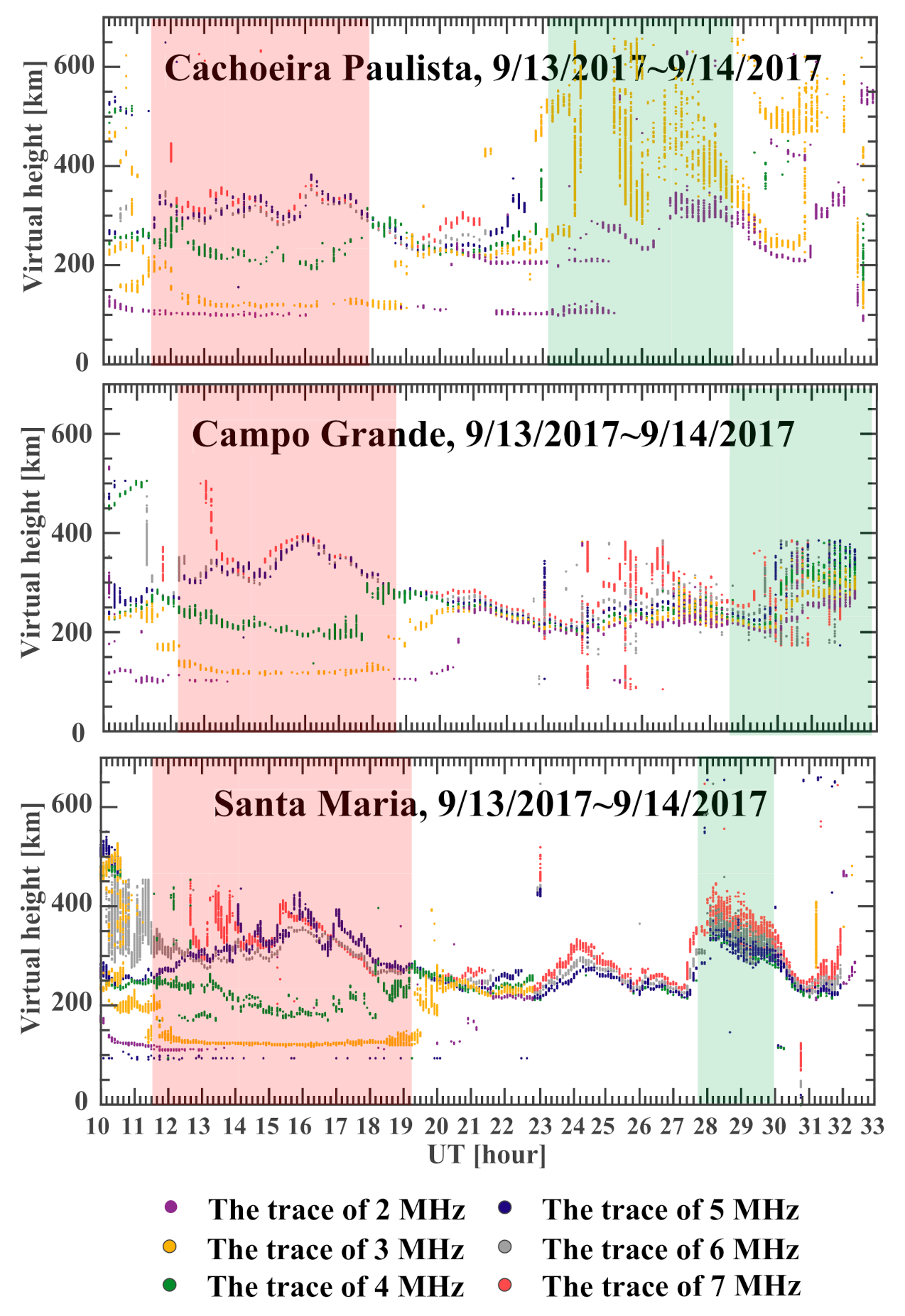
Multi-hop traces are present on the ionograms, which represent radio waves reflected by the ground. The upper trace in Figure 2d, which is called the second-hop trace, was not required in this work because it is the replicate of the one-hop trace of O wave. It is well known that the height of the second-hop trace is twice that of the one-hop trace, so the one-hop trace can be easily distinguished from the second-hop trace according to the distinct height difference between them. The extracted one-hop trace is presented in Figure 2e.
(5)
Then, a morphological erosion operation was used to eliminate the effect of some noise pixels which were close to the main trace, as shown in Figure 2f.
(6)
Finally, morphological thinning was applied, making it possible to obtain more accurate height values of the O-wave trace from the ionograms. The final O-wave trace is presented in Figure 2h.
In this study, all ionograms were processed following the same processing steps. Moreover, if the ionograms contained a large number of diffusion effects, some of the diffusion pixels (which indicate the spread-F phenomenon) will remain in the ionograms rather than a thin line after processing, as shown in Figure 2h.
In the large number of ionograms, such as those shown in Figure 2, we noticed that there was always a black trace drawn on the ionograms, indicating the O-wave trace. By extracting this black trace from the ionograms, we could examine the validity of the O-wave trace obtained by digital image processing. Using the ionograms collected from Cachoeira Paulista during September 2017 to obtain the examined result, the root-mean-square error (RMSE) of frequency–virtual height curves is shown in Figure 3. The result shows that the technique we applied produces larger errors in the low frequency zone, especially when the frequency is less than 2 MHz, which is probably caused by the wave trace of the ionospheric E region, whereas the errors in the high frequency region are relatively small and stable. Because we are concerned with the higher frequencies, especially those of 4, 5, 6, and 7 MHz, the indicated techniques are effective.
By consecutively recording how the virtual height of the extracted O-wave trace at certain key frequencies, such as 2, 3, 4, 5, 6, and 7 MHz, fluctuated over 48 h, further analysis was carried out. The O-wave traces corresponding to each frequency are shown in Figure 4 and Figure 7, which are depicted by isolating the corresponding pixels of each frequency directly. These figures not only essentially indicate the O-wave trace variations, but also show the spread-F occurrence during the day and night. In Figure 4 and Figure 7, the traces fluctuating with a certain period show the occurrence of a typical MSTID, and the corresponding region is highlighted in red, whereas the corresponding diffuse pixels in the figures represent a typical spread-F event, which is highlighted in green. By setting a threshold to filter the possible clutter echo, we can identify 209 days with spread-F occurrence out of 367 recorded days. Further statistical analysis is shown in the following.
In this study, the three-channel maximum entropy method (MEM) was utilized to calculate the characteristics of MSTID, such as the frequency, phase velocity, wave number, and azimuth. A detailed introduction to the MEM method is provided in [33,34]. The calculation process of MSTID parameters is given as follows:
First, we selected the TEC data from three GPS stations. On the basis of MEM theory, the spatial position of the three GPS stations needs to satisfy the non-collinearity principle. The TEC data used in this study from the CHPG, CHPI, and UFPR stations meet the requirements.
Second, we needed to obtain the TEC disturbance from the background TEC data. In this study, a running window with a time interval of 2 min and a length of 1.2 h was used to preprocess the time series of TEC data to produce a series of TEC data with a length of 1.2 h. Then, using the least squares method, the TEC disturbance data were obtained from the 1.2 h time series of TEC. In this work, the maximum amplitude of TEC disturbances exceeding 2 TECU (1 TECU = 1016 electrons/m2) were considered MSTID events in our study. Thus, we were able to obtain 1119 valid MSTID events during the period of April 2017–April 2018.
Third, the MEM method was applied to TEC disturbance data from three GPS stations to calculate the key parameters of MSTID. The MEM method can be described using the following equation: f , ϕ 21 , ϕ 31 = M E M I 1 , I 2 , I 3 , in which f, ϕ21, ϕ31, I1, I2, I3 are the MSTID frequency, the phase difference between station 1 and station 2, the phase difference between station 1 and station 3, and the ΔTEC time series observed by three stations at the same time, respectively. The indicated phase difference can be calculated using following equation:
ϕ f = arctan i m a g P x y f r e a l P x y f
where Pxy is the cross-power spectrum of the two stations. After obtaining these parameters, we can compute the wave number k of the indicated propagation pattern:
k x = y 21 ϕ 31 y 31 ϕ 21 x 31 ϕ 21 x 21 ϕ 31
k y = x 21 ϕ 31 x 31 ϕ 21 y 31 ϕ 21 y 21 ϕ 31
k = k x 2 + k y 2
Furthermore, we can obtain more key parameters, such as horizontal phase speed vph and wave propagation azimuth σ, according to the following equations:
v p h = 2 π f k
σ = a r e tan k x k y
Due to the limitation of sampling frequency, we cannot determine the main frequency of MSTID. However, because the azimuth σ is robust to a range of frequencies during a MSTID event, we were able to compute the mean azimuth σ for a range of frequencies.
In the process of statistical analysis of the data recorded from April 2017 to April 2018, we found that MSTID can trigger the spread-F. We selected two typical cases to demonstrate the relationship between MSTID and spread-F.

3. Results

Figure 4 shows the variation of the virtual heights at different plasma frequencies extracted from the ionograms taken from three ionosonde stations. As shown in Figure 4, the red region shows clear fluctuations representing significant MSTID characteristics, whereas the green region shows noteworthy spread-F characteristics. Moreover, we utilized the ΔTEC time series recorded at the three IGS stations, as shown in Figure 5, to further examine and compute the MSTID variation parameters; the indicated result is shown in Figure 6. The region highlighted by the red color indicates the MSTID occurrence. During the recorded MSTID occurrence, which lasted approximately 42 min, the average frequency, the average phase velocity, the average wave number, and the average azimuth were 4.0579 h−1, 725.3989 km/h, 0.0320 rad/km, and −0.8771 rad (309.746°), respectively, suggesting a northwestward propagation. Using the same analysis techniques, we analyzed a similar case recorded on 13 September 2017. The traces of the ionograms are shown in Figure 7, and indicate that spread-F occurrence may have been triggered by the previous MSTID occurrence. More accurate parameters can be computed with the TEC data. With the ΔTEC traces shown in Figure 8, we can acquire the specified parameters.
As shown in Figure 9, with the indicated MEM, we could acquire the accurate MSTID frequency f, phase speed vph, wave number k, and propagation azimuth σ during an MSTID occurrence that lasted approximately 52 min, and their average values were 1.5524 h−1, 683.33 km/h, 0.0146 rad/km and −1.0269 rad (301.163°), respectively, suggesting a northwestward propagation of MSTID. Figure 9 indicates how the stated parameters varied over time during an MSTID occurrence case.
In summary, from Figure 4, Figure 5, Figure 6, Figure 7, Figure 8 and Figure 9, we report the MSTID and spread-F events observed by ionosondes and GPS stations in South America. These observational results demonstrate that nighttime MSTID may be the possible source of the generation of spread-F.

4. Statistical Analysis

With the same techniques we employed in the case study, we were able to perform statistical analysis with the ionogram data and the IGS data during April 2017–April 2018 to explore further possible connections between MSTID and spread-F.
Throughout the total observed period from April 2017 to April 2018 over the station Cachoeira Paulista in South America, the ionosondes mentioned above recorded valid ionograms data on 367 days, of which the spread-F was observed on 209 days. Furthermore, we analyzed the TEC data collected from CHPG, CHPI, and UFPR stations. The seasonal distributions of the spread-F and MSTID occurrence are shown in Figure 10. From the figure, we may note that MSTID was significantly more frequent in spring and summer, and much less frequent during winter, whereas spread-F occurrence was slightly more frequent in autumn and winter. With this inversely distributed occurrence rate of spread-F and MSTID, we assume that a certain type of MSTID has a greater possibility to trigger spread-F. Further analysis is elaborated in the following.
Then, we analyzed the variations of spread-F and MSTID occurrence distribution with local time, and the result is shown in Figure 11. It can be seen from the indicated figure that the MSTID around midnight has a high possibility of triggering spread-F. Due to the results of the below analysis of the azimuth of the MSTID propagation, which is generally northwestward, we naturally assume that the major source of MSTID is the Perkins instability. Perkins instability is generally associated with polarization electric field, which is believed to account for the post-midnight F-layer instabilities.
By eliminating the data with no MSTID occurrence before the spread-F occurrence, we can locate the MSTID occurrence that may trigger a spread-F event and perform further statistical analysis on the key parameters of the MSTID, including MSTID main frequency f, occurrence local time, ΔTEC maximum amplitude, phase speed vph, wave number k, and propagation azimuth σ, using MEM on 1119 cases throughout a year. The indicated result is shown in Figure 12.
Figure 12 shows that during April 2017–April 2018 of the indicated region of South America, the MSTID main frequency was mainly below 0.5 h−1, the TID ΔTEC amplitude was mainly below 4, the major azimuth was basically between −1 and −0.7 rad, and the velocity speed varies mainly between 0 and 2000 km/h.
Combining the results in Figure 11 and Figure 12, we suppose that MSTID occurrence is highly likely to trigger spread-F. Moreover, according to the above statistical analysis, TID that is apt to trigger a spread-F event is generally characterized by larger ΔTEC amplitude, propagation azimuth around −1 rad, wave number around 0.005 rad/km, and phase speed around 1000 km/h.

5. Discussion and Conclusions

To examine the theory that MSTID may seed spread-F occurrences, we investigated the MSTID and spread-F occurrence in the South America region from April 2017 to April 2018. As shown in Figure 11, spread-F occurrence is most common around midnight, which is consistent with the work of [35]. This may due to the preferable conditions for Rayleigh–Taylor instability during nighttime. There are several factors that have been investigated in several previous studies, such as the smaller neutral density during nighttime, pre-reversal enhancement, solar activity, and altitude of the F-layer height [36,37]. However, limited research has investigated the underlying factors of MSTID that trigger spread-F occurrence. MSTID can be excited in two approaches: by gravity waves or by Perkins instability. It is generally acknowledged that TID may seed spread-F occurrence through polarization electric fields. Previous research has conclusively determined that polarization electric fields can trigger Rayleigh–Taylor instability and thus induce spread-F occurrence [15,19,20]. According to the previous study of Miller, MSTID triggered by atmosphere gravity waves play a role in the seeding of F-layer irregularities [38]. However, unlike MSTID triggered by gravity waves, in which polarization electric fields initiate under favorable circumstances [15], the MSTID triggered by Perkins instability is generally accompanied by polarization electric fields to maintain a divergence-free ionospheric current. Therefore, we assume that MSTID triggered by Perkins instability would show a further tendency to trigger spread-F occurrence.
Through a statistical analysis of the seasonal distribution of MSTID and spread-F, the result in Figure 10 indicates that MSTID is significantly more common in spring and summer, and much less frequent during winter, whereas spread-F is more frequent in autumn and winter. This is consistent with many studies that suggest that MSTIDs are more common in summer, especially at nighttime, taking into account the seasonal difference between northern and southern hemispheres. From the inverse seasonal variation of the occurrence rate of MSTID and spread-F, we assumed that, although it is generally acknowledged that MSTID plays a role in inducing the spread-F occurrence, some types of MSTID are noticeably more likely to trigger spread-F. One factor we take into account is how the MSTID is excited; we assume MSTID triggered by Perkins instability generally increases the tendency to trigger spread-F. MSTID triggered by Perkins instability in the southern hemisphere generally shows a northwestward propagation pattern. We studied the MSTID azimuth distribution in the South America region, which is shown in Figure 12. The main azimuth is northwestward, which is consistent with the stated principle of the MSTID azimuth distribution.
We studied the MSTID occurrence at midnight and found MSTID occurring post-midnight had a clearly greater possibility of triggering spread-F occurrence. Because Perkins instability only occurs during nighttime and the favorable conditions for F-layer instability, such as PRE, occur during post-sunset, we assume this peak possibility distribution is seeded by midnight polarization electric fields, triggering Rayleigh–Taylor instability and the formation of plasma bubbles.
However, according to the statistical analysis, there exist several cases of daytime spread-F occurrence which are not likely to be triggered by MSTID seeded by Perkins instability. We conjecture this may be triggered by gravity waves. Although there was a lack of favorable conditions, such as PRE, to trigger Rayleigh–Taylor instability, oscillation of neutral air, which excites ion-neutral collisions, may be a reason for the daytime spread-F occurrences [20].
As shown in Figure 12, according to the statistical analysis in which the days with no MSTID occurrence before spread-F occurrence were eliminated, MSTIDs that tend to trigger spread-F are generally characterized by larger ΔTEC amplitudes, propagation azimuth around −1 rad, wave number around 0.005 rad/km, and phase speed around 1000 km/h, which is consistent with the research of other scholars. Using subtle phase-path measurements for the equatorial region, [39] shows that MSTID wave amplitudes become larger when spread-F exists [40].
Based on the above discussion, our results are generally consistent with previous studies with different measurements. However, there are some new findings worth noting, which can be summarized as follows:
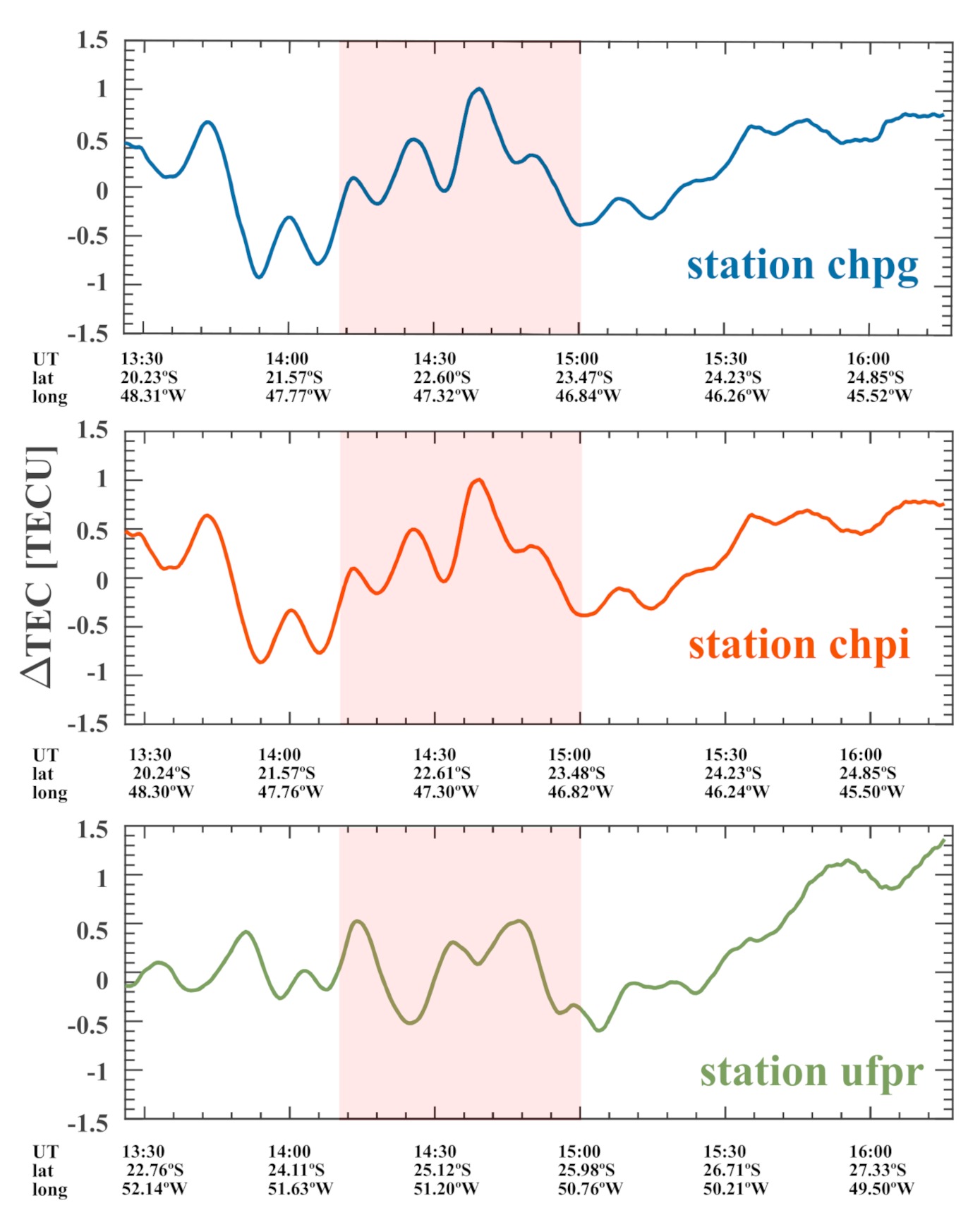
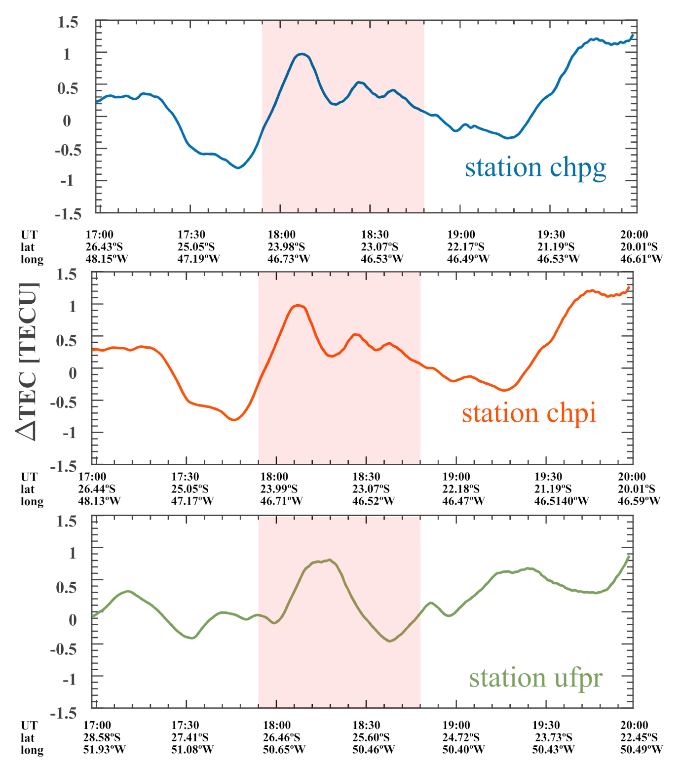
  • The cases of MSTIDs observed in the South America region generally manifest a northwestward prorogating pattern, which may suggest the majority of the observed MSTIDs are triggered by Perkins instability.
  • Nighttime MSTIDs in the South America region have high possibilities according to statistical analysis. Assuming these are caused by Perkins instability, the phenomenon is consistent with the post-midnight F-layer instability being caused by the polarization electric field, which often initiates during a MSTID event triggered by Perkins instability.
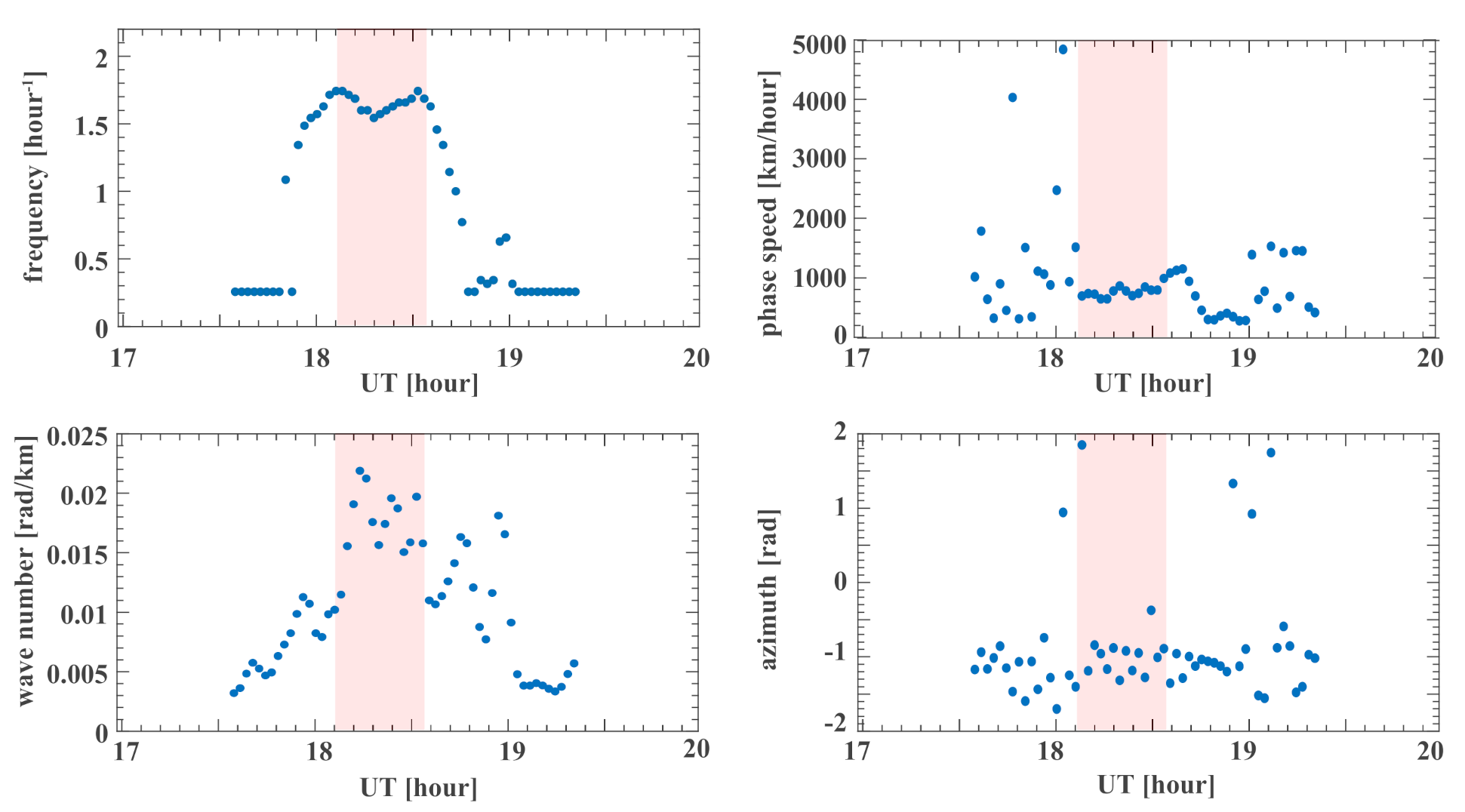
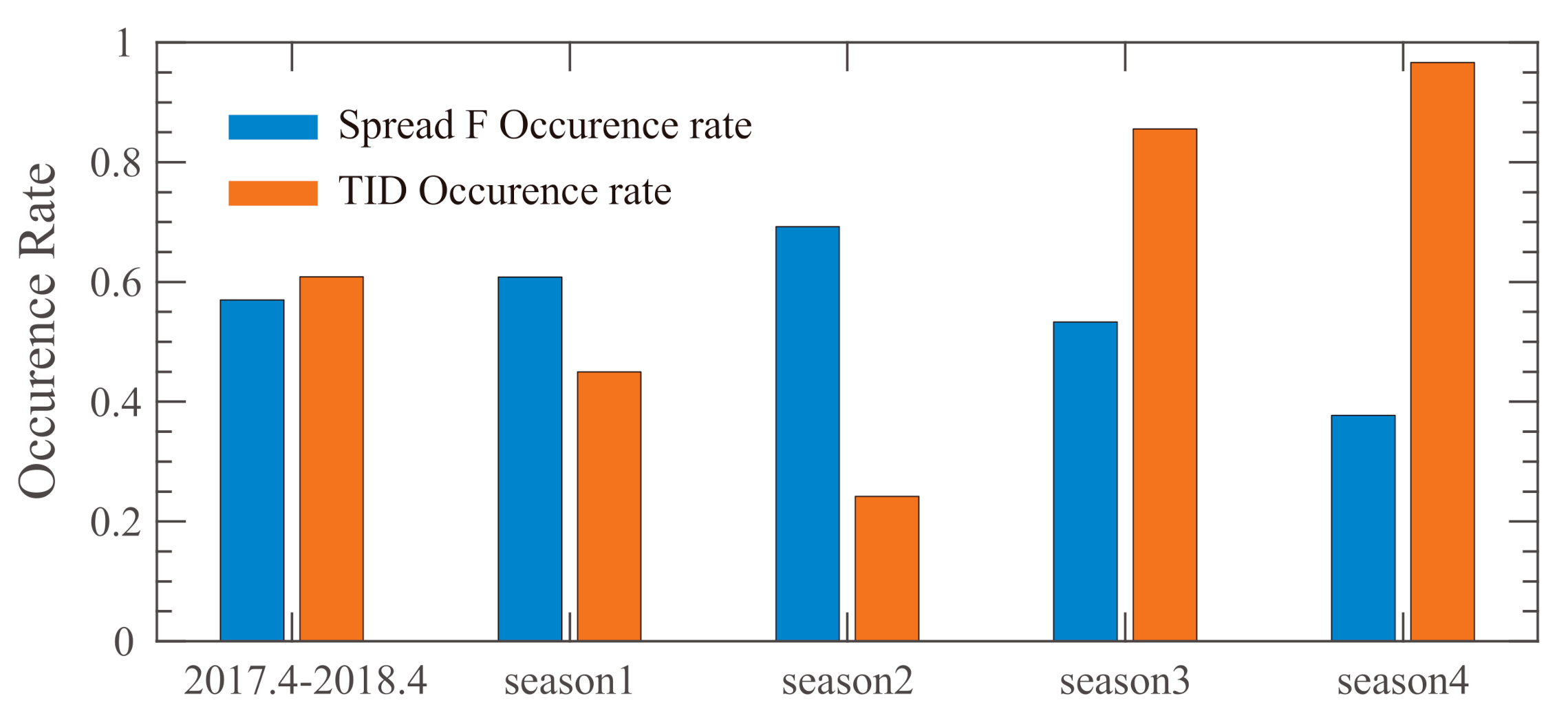
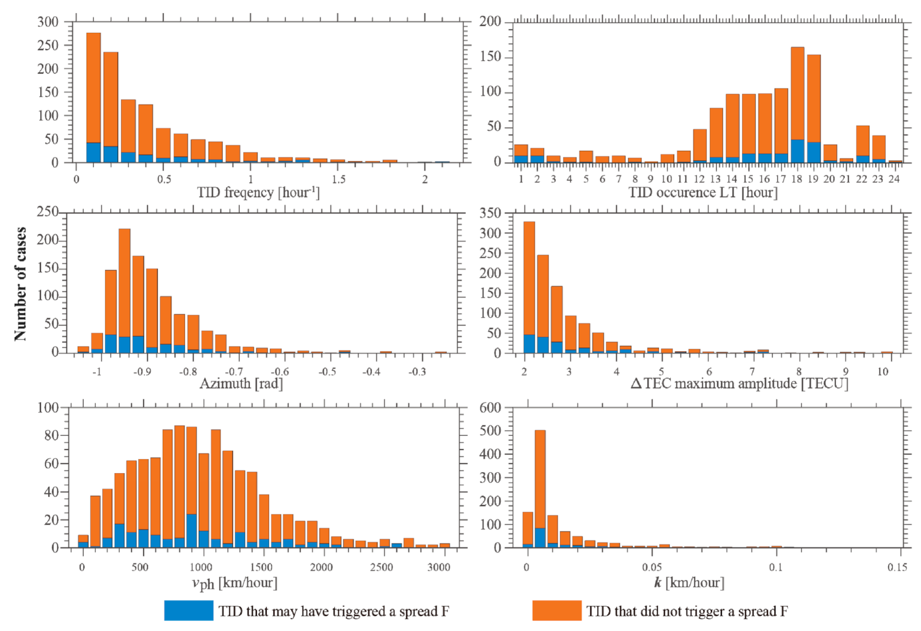
  • The inversely seasonal variation of MSTID and spread-F occurrence may suggest that certain types of MSTID generally have a higher possibility of triggering spread-F. MSTIDs that tend to trigger spread-F in the South America region are generally characterized by larger ΔTEC amplitudes, a phase speed around 900 km/h, and an azimuth between −1 rad and −0.9 rad. Further research should explore this topic.

Author Contributions

Conceptualization, Z.D., Y.L. and C.Z.; methodology, R.W.; investigation, T.X.; validation, Z.W. and G.C.; formal analysis, Y.L.; resources, C.Z.; visualization, Q.T. and Z.X.; funding acquisition, Y.L. All authors have read and agreed to the published version of the manuscript.

Funding

This work was supported by the Taishan Scholars Project of Shandong Province under Grant No. ts20190968, the National Natural Science Foundation of China (NSFC grant No.41574146 and 41774162), the National Key R&D Program of China (Grant No. 2018YFC1503506), the foundation of National Key Laboratory of Electromagnetic Environment (Grant No. 6142403180204), and Excellent Youth Foundation of Hubei Provincial Natural Science Foundation (Grant No. 2019CFA054).

Data Availability Statement

The use of ionosonde data provided by Lowell Digisonde International (https://www.digisonde.com/ accessed on 1 April 2017). The use of GPS data provided by IGS Data Center (http://www.igs.org/ accessed on 1 April 2017).

Acknowledgments

We acknowledge the use of ionosonde data provided by Lowell Digisonde International (https://www.digisonde.com/ accessed on 1 April 2017). We also are thankful for the use of GPS data provided by IGS Data Center (http://www.igs.org/ accessed on 1 April 2017).

Conflicts of Interest

The authors declare no conflict of interest.

References

  1. Ratcliffe, J.A. Introduction to the Ionosphere and Magnetosphere; Cambridge University Press: Cambridge, UK, 1972. [Google Scholar]
  2. Petrík, T.; Daneček, M.; Uhlíř, I.; Poulek, V.; Libra, M. Distribution Grid Stability—Influence of Inertia Moment of Synchronous Machines. Appl. Sci. 2020, 10, 9075. [Google Scholar] [CrossRef]
  3. Alfonsi, L.; Spogli, L.; Pezzopane, M.; Romano, V.; Zuccheretti, E.; De Franceschi, G.; Ezquer, R.G. Comparative analysis of spread-F signature and GPS scintillation occurrences at Tucumán, Argentina. J. Geophys. Res. Space Phys. 2013, 118, 4483–4502. [Google Scholar] [CrossRef] [Green Version]
  4. Abdu, M.A.; De Medeiros, R.T.; Bittencourt, J.A.; Batista, I.S. Vertical ionization drift velocities and range type spread F in the evening equatorial ionosphere. J. Geophys. Res. Space Phys. 1983, 88, 399–402. [Google Scholar] [CrossRef] [Green Version]
  5. Kelley, M.C.; McClure, J.P. Equatorial spread-F: A review of recent experimental results. J. Atmos. Terr. Phys. 1981, 43, 427–435. [Google Scholar] [CrossRef]
  6. Tsunoda, R.T. Control of the seasonal and longitudinal occurrence of equatorial scintillations by longitudinal gradient in integrated E region Pedersen conductivity. J. Geophys. Res. Space Phys. 1985, 90, 447–456. [Google Scholar] [CrossRef]
  7. Otsuka, Y.; Ogawa, T. VHF radar observations of nighttime F-region field-aligned irregularities over Kototabang, Indonesia. Earth Planets Space 2009, 61, 431–437. [Google Scholar] [CrossRef] [Green Version]
  8. Lloyd, K.H.; Haerendel, G. Numerical modeling of the drift and deformation of ionospheric plasma clouds and of their interaction with other layers of the ionosphere. J. Geophys. Res. 1973, 78, 7389–7415. [Google Scholar] [CrossRef]
  9. Farley, D.T.; Balsey, B.B.; Woodman, R.F.; McClure, J.P. Equatorial spread F: Implications of VHF radar observations. J. Geophys. Res. 1970, 75, 7199–7216. [Google Scholar] [CrossRef]
  10. Rao, P.R.; Ram, S.T.; Niranjan, K.; Prasad, D.S.V.V.D.; Krishna, S.G.; Lakshmi, N.K.M. VHF and L-band scintillation characteristics over an Indian low latitude station, Waltair (17.7°N, 83.3°E). Ann. Geophys. 2005, 23, 2457–2464. [Google Scholar]
  11. Fagundes, P.R.; Abalde, J.R.; Bittencourt, J.A.; Sahai, Y.; Francisco, R.G.; Pillat, V.G.; Lima, W.L.C. F layer postsunset height rise due to electric field prereversal enhancement: 2. Traveling planetary wave ionospheric disturbances and their role on the generation of equatorial spread F. J. Geophys. Res. Space Phys. 2009, 114. [Google Scholar] [CrossRef] [Green Version]
  12. Huang, C.S.; Hairston, M.R. The postsunset vertical plasma drift and its effects on the generation of equatorial plasma bubbles observed by the C/NOFS satellite. J. Geophys. Res. Space Phys. 2015, 120, 2263–2275. [Google Scholar] [CrossRef]
  13. Huang, C.S. Plasma drifts and polarization electric fields associated with TID-like disturbances in the low-latitude ionosphere: C/NOFS observations. J. Geophys. Res. Space Phys. 2016, 121, 1802–1812. [Google Scholar] [CrossRef] [Green Version]
  14. Huang, C.S. The characteristics and generation mechanism of small-amplitude and large-amplitude ESF irregularities observed by the C/NOFS satellite. J. Geophys. Res. Space Phys. 2017, 122, 8959–8973. [Google Scholar] [CrossRef]
  15. Kelley, M.C.; Miller, C.A. Electrodynamics of midlatitude spread F 3. Electrohydrodynamic waves? A new look at the role of electric fields in thermospheric wave dynamics. J. Geophys. Res. Space Phys. 1997, 102, 11539–11547. [Google Scholar] [CrossRef]
  16. Hocke, K.; Schlegel, K. A review of atmospheric gravity waves and travelling ionospheric disturbances: 1982–1995. Ann. Geophys. 1996, 14, 917–940. [Google Scholar]
  17. Hocke, K.; Schlegel, K.; Kirchengast, G. Phases and amplitudes of TIDs in the high latitude F-region observed by EISCAT. J. Atmos. Terr. Phys. 1996, 58, 245–255. [Google Scholar] [CrossRef]
  18. Miller, E.S.; Makela, J.J.; Kelley, M.C. Seeding of equatorial plasma depletions by polarization electric fields from middle latitudes: Experimental evidence. Geophys. Res. Lett. 2009, 36. [Google Scholar] [CrossRef]
  19. Balan, N.; Shiokawa, K.; Otsuka, Y.; Kikuchi, T.; Vijaya Lekshmi, D.; Kawamura, S.; Bailey, G.J. A physical mechanism of positive ionospheric storms at low latitudes and midlatitudes. J. Geophys. Res. Space Phys. 2010, 115. [Google Scholar] [CrossRef]
  20. Oliver, W.L.; Otsuka, Y.; Sato, M.; Takami, T.; Fukao, S. A climatology of F region gravity wave propagation over the middle and upper atmosphere radar. J. Geophys. Res. Space Phys. 1997, 102, 14499–14512. [Google Scholar] [CrossRef]
  21. Kelley, M.C.; Makela, J.J.; Swartz, W.E.; Collins, S.C.; Thonnard, S.; Aponte, N.; Tepley, C.A. Caribbean Ionosphere Campaign, year one: Airglow and plasma observations during two intense mid-latitude spread-F events. Geophys. Res. Lett. 2000, 27, 2825–2828. [Google Scholar] [CrossRef]
  22. Bowman, G.G. A review of some recent work on mid-latitude spread-F occurrence as detected by ionosondes. J. Geomagn. Geoelectr. 1990, 42, 109–138. [Google Scholar] [CrossRef] [Green Version]
  23. Subbarao, K.S.V.; Murthy, B.K. Post-sunset F-region vertical velocity variations at magnetic equator. J. Atmos. Terr. Phys. 1994, 56, 59–65. [Google Scholar] [CrossRef]
  24. Subbarao, K.S.V.; Murthy, B.K. Seasonal variations of equatorial spread-F. Ann. Geophys. 1994, 12, 33–39. [Google Scholar] [CrossRef]
  25. Lan, T.; Jiang, C.; Yang, G.; Zhang, Y.; Liu, J.; Zhao, Z. Statistical analysis of low-latitude spread F observed over Puer, China, during 2015-2016. Earth Planets Space 2019, 71, 138. [Google Scholar] [CrossRef]
  26. Bowman, G.G. Nighttime mid-latitude travelling ionospheric disturbances associated with mild spread-F conditions. J. Geomagn. Geoelectr. 1991, 43, 899–920. [Google Scholar] [CrossRef]
  27. Morton, F.W.; Essex, E.A. Gravity wave observations at a southern hemisphere mid-latitude station using the total electron content technique. J. Atmos. Terr. Phys. 1978, 40, 1113–1122. [Google Scholar] [CrossRef]
  28. Tsugawa, T.; Otsuka, Y.; Coster, A.J.; Saito, A. Medium-scale traveling ionospheric disturbances detected with dense and wide TEC maps over North America. Geophys. Res. Lett. 2007, 34. [Google Scholar] [CrossRef]
  29. Ding, F.; Wan, W.; Xu, G.; Yu, T.; Yang, G.; Wang, J.S. Climatology of medium-scale traveling ionospheric disturbances observed by a GPS network in central China. J. Geophys. Res. Space Phys. 2011, 116. [Google Scholar] [CrossRef]
  30. Otsu, N. A threshold selection method from gray-level histograms. IEEE Trans. Syst. 1979, 9, 62–66. [Google Scholar] [CrossRef] [Green Version]
  31. Smith, R. Hybrid Page Layout Analysis via Tab-Stop Detection. In Proceedings of the 10th International Conference on Document Analysis and Recognition, Barcelona, Spain, 26–29 July 2009. [Google Scholar]
  32. Smith, R. An overview of the tesseract OCR engine. In Proceedings of the Ninth International Conference on Document Analysis and Recognition (ICDAR 2007), Curitiba, Brazil, 23–26 September 2007. [Google Scholar]
  33. Wang, M.; Ding, F.; Wan, W.; Ning, B.; Zhao, B. Monitoring global traveling ionospheric disturbances using the worldwide GPS network during the October 2003 storm. Earth Planets Space 2007, 59, 1–13. [Google Scholar] [CrossRef] [Green Version]
  34. Chen, G.-Y.; Zhou, C.; Liu, Y.; Zhao, J.; Tang, Q.; Wang, X.; Zhao, Z. A statistical analysis of medium-scale traveling ionospheric disturbances during 2014–2017 using the Hong Kong CORS network. Earth Planets Space 2019, 71, 1–14. [Google Scholar] [CrossRef]
  35. Candido, C.M.N.; Batista, I.S.; Becker-Guedes, F.; Abdu, M.A.; Sobral, J.H.A.; Takahashi, H. Spread F occurrence over a southern anomaly crest location in Brazil during June solstice of solar minimum activity. J. Geophys. Res. Space Phys. 2011, 116. [Google Scholar] [CrossRef] [Green Version]
  36. Kelley, M.C.; Hysell, D.L. Equatorial spread-F and neutral atmospheric turbulence: A review and a comparative anatomy. J. Atmos. Terr. Phys. 1991, 53, 695–708. [Google Scholar] [CrossRef]
  37. Otsuka, Y.; Nishioka, M.; Shiokawa, K.; Nagatsuma, T.; Tsugawa, T.; Perwitasari, S. Post-midnight field-aligned irregularities observed with a VHF radar at Kototabang, Indonesia. In AGU Fall Meeting Abstracts; American Geophysical Union: San Francisco, CA, USA, 2011. [Google Scholar]
  38. Miller, C.A.; Swartz, W.E.; Kelley, M.C.; Mendillo, M.; Nottingham, D.; Scali, J.; Reinisch, B. Electrodynamics of midlatitude spread F: 1. Observations of unstable, gravity wave-induced ionospheric electric fields at tropical latitudes. J. Geophys. Res. Space Phys. 1997, 102, 11521–11532. [Google Scholar] [CrossRef]
  39. Rao, D.G.; Bhattacharya, G.C.; Ramana, M.V.; Subrahmanyam, V.; Ramprasad, T.; Krishna, K.S.; Reddy, S.I. Analysis of multi-channel seismic reflection and magnetic data along 13 N latitude across the Bay of Bengal. Mar. Geophys. Res. 1994, 16, 225–236. [Google Scholar] [CrossRef]
  40. Bowman, G.G. Multiplicity of travelling disturbances in the nighttime mid-latitude F 2-region ionosphere. Indian J. Radio Space Phys. 1995, 24, 91–96. [Google Scholar]
Figure 1. Geographic locations of the ionosonde stations and the GPS stations in South America.
Remotesensing 13 00945 g001
Figure 2. Procedure of O-wave trace extraction in ionograms. (a) Original ionogram, (b) color extraction, (c) morphological dilation, (d) trace connectivity labeling and filtering noise, (e) removing the second-hop, (f) morphological erosion, (g) morphological thinning, (h) the obtained O-wave trace from the ionogram.
Remotesensing 13 00945 g002
Figure 3. The RMSE computed with the extracted O-wave trace with the morphological processing perspective and the extracted black trace. The outcome of the examined section was obtained using 4394 ionograms collected from Cachoeira Paulista during September 2017.
Remotesensing 13 00945 g003
Figure 4. The case with traces extracted from the ionograms collected from 21 August 2017 to 22 August 2017. Each row of traces shown in the figure are recorded by the ionosondes at Cachoeira Paulista, Campo Grande, and Santa Mari. The listed figures all show a specific pattern: medium-scale traveling ionospheric disturbance (MSTID) variation followed by typical nighttime spread-F occurrence.
Remotesensing 13 00945 g004
Figure 5. Time series of ΔTEC recorded by CHPG, CHPI, and UFPR stations during 21 August 2017.
Remotesensing 13 00945 g005
Figure 6. MSTID parameters calculated by TEC time series recorded by CHPG, CHPI, and UFPR stations during 21 August 2017.
Remotesensing 13 00945 g006
Figure 7. The case with traces extracted from the ionograms collected from 13 September 2017 to 14 September 2017. Each row of traces shown in the figure are recorded by the ionosondes located in Cachoeira Paulista, Campo Grande, and Santa Maria, respectively. The listed figures all show a specific pattern—MSTID variation followed by typical nighttime spread-F occurrence.
Remotesensing 13 00945 g007
Figure 8. Time series of ΔTEC recorded by CHPG, CHPI, and UFPR stations during 21 August 2017.
Remotesensing 13 00945 g008
Figure 9. MSTID parameters calculated by TEC time series recorded by CHPG, CHPI, and UFPR stations during 21 August 2017.
Remotesensing 13 00945 g009
Figure 10. The seasonal distribution of the occurrence rate of MSTID and spread-F. Season 1, 2, 3, and 4 refer to autumn, winter, spring, and summer, respectively, in the southern hemisphere.
Remotesensing 13 00945 g010
Figure 11. The local time variations of MSTID occurrence rate and spread-F occurrence rate.
Remotesensing 13 00945 g011
Figure 12. The statistical analysis of the key parameters of MSTID, namely, MSTID main frequency f, occurrence local time LT, ΔTEC maximum amplitude, phase speed vph, wave number k, and propagation azimuth σ.
Remotesensing 13 00945 g012
Publisher’s Note: MDPI stays neutral with regard to jurisdictional claims in published maps and institutional affiliations.

