
Hyperspectral Image Clustering with Spatially-Regularized Ultrametrics


1
Department of Computer Science, Tufts University, Medford, MA 02155, USA
2
Department of Mathematics, Tufts University, Medford, MA 02155, USA
*
Author to whom correspondence should be addressed.
Remote Sens. 2021, 13(5), 955; https://0-doi-org.brum.beds.ac.uk/10.3390/rs13050955
Submission received: 8 January 2021
/
Revised: 23 February 2021
/
Accepted: 2 March 2021
/
Published: 4 March 2021
(This article belongs to the Special Issue Theory and Application of Machine Learning in Remote Sensing)
Abstract
:We propose a method for the unsupervised clustering of hyperspectral images based on spatially regularized spectral clustering with ultrametric path distances. The proposed method efficiently combines data density and spectral-spatial geometry to distinguish between material classes in the data, without the need for training labels. The proposed method is efficient, with quasilinear scaling in the number of data points, and enjoys robust theoretical performance guarantees. Extensive experiments on synthetic and real HSI data demonstrate its strong performance compared to benchmark and state-of-the-art methods. Indeed, the proposed method not only achieves excellent labeling accuracy, but also efficiently estimates the number of clusters. Thus, unlike almost all existing hyperspectral clustering methods, the proposed algorithm is essentially parameter-free.
1. Introduction
Remote sensing image processing has been revolutionized by machine learning, in particular the labeling of material classes in remotely sensed images. This can take the form of supervised classification, when many labeled pixels are available to help guide the algorithm, or unsupervised clustering, when no labeled pixels are available to the algorithm. When large labeled training sets are available, supervised methods such as kernel methods [1,2,3] and deep neural networks [4,5,6] accurately label pixels in a wide range of imaging modalities. However, it is often impractical to acquire the large training sets necessary for these methods to work well. When human-annotated data is limited, it is necessary to develop unsupervised clustering methods which label the entire data set without the need for training data.
Unsupervised clustering is a classical problem in machine learning, and many methods for unsupervised clustering have been proposed [7]. However, most only enjoy theoretical performance guarantees under very restrictive assumptions on the underlying data. For example, K-means clustering works well for clusters that are roughly spherical and well-separated, but provably fails when the clusters become nonlinear or poorly separated [8]. Clustering methods based on deep learning may perform well in some instances, but are sensitive to metaparameters and lack robust mathematical performance guarantees even in highly idealized settings [9,10,11].
Clustering of remotely sensed hyperspectral images (HSI) is particularly challenging, due to their high-dimensionality, noise, and often poor spatial resolution. Moreover, most existing HSI clustering methods require the number of clusters to be input as a parameter to the algorithm, which is impractical in the unsupervised setting. Despite their challenges, unsupervised HSI clustering methods are increasingly important, because the lack of large training sets prevents supervised learning from being effective on the deluge of HSI data being collected.
Recently, ultrametric path distances (UPD) have been proven to provide state-of-the-art theoretical results for clustering high-dimensional data [12]. In particular, only very weak assumptions on the data are required, namely that the underlying clusters exhibit intrinsically low-dimensional structure and are separated by regions of low density. This suggests UPD are well-suited for HSI [13], which while very high-dimensional, are typically such that each class in the data depends (perhaps nonlinearly) on only a small number of latent variables, and in this sense are intrinsically low-dimensional.
In this paper, we develop an HSI clustering algorithm based on ultrametric spectral clustering. Taking advantage of recent theoretical developments, our approach constructs a weighted graph with nodes corresponding to HSI pixels and edge weights determined by the UPD metric. Crucially, the proposed method spatially regularizes the graph in order to capture important spatial correlations in the HSI. After constructing this spatially regularized UPD graph, the proposed method runs K-means clustering on the lowest frequency eigenfunctions of the graph Laplacian. We call the proposed method spatially regularized ultrametric spectral clustering (SRUSC). SRUSC scales quasilinearly in the number of data points, and has few tunable parameters. Moreover, the proposed method outperforms a range of benchmark and state-of-the-art unsupervised and even supervised classification methods on several synthetic and real HSI in terms of clustering accuracy and efficient estimation of the number of latent clusters. The detection of the number of clusters is particularly significant, because it makes the proposed method essentially parameter-free, unlike nearly all existing methods for clustering HSI.
To summarize, this paper makes three major contributions:
- We propose the SRUSC algorithm for HSI clustering. This method enjoys rich theoretical justification and is intuitively simple, with few sensitive parameters to tune. In particular, SRUSC detects the number of clusters in the HSI.
- We prove performance guarantees on the runtime of SRUSC. This ensures fast performance of SRUSC on high-dimensional data that exhibits intrinsically low-dimensional structure, allowing the proposed method to scale.
- We demonstrate that SRUSC effectively clusters synthetic and real HSI with higher accuracy than a range of benchmark and state-of-the-art methods. Moreover, we show that SRUSC efficiently estimates the number of clusters in these datasets, thereby addressing a major outstanding problem in the HSI clustering literature.
The remainder of this article is organized as follows. In Section 2, we provide background on unsupervised HSI clustering and ultrametric path distances. In Section 3, we motivate and detail the proposed algorithm and discuss its theoretical properties and complexity. In Section 4, we introduce several data sets and perform comparisons between the proposed method and related methods, demonstrating the strong performance of SRUSC not only compared to state-of-the-art unsupervised methods, but compared to supervised methods as well. This section investigates both clustering accuracy and estimation of the number of clusters. We conclude and discuss potential directions for future research in Section 5.
2. Background
We present a problem statement and background on clustering in Section 2.1 before reviewing UPD and spectral clustering in Section 2.2 and Section 2.3, respectively.
2.1. Background on Unsupervised Clustering
The problem of unsupervised clustering consists in providing a data set with natural group labels corresponding to clusters formed by the data points. Mathematically, there is a set of latent labels , where each and K is the number of latent classes in X. The goal of unsupervised clustering is to learn these labels given X alone; in particular, no training pairs of the form are provided to guide the process. So, labeling decisions must be made entirely based on latent geometrical and statistical properties of the data. The lack of training pairs of the form is the primary challenge of unsupervised clustering, and differentiates it from supervised classification.
A range of methods for clustering data have been developed, including K-means clustering and Gaussian mixture models, which assume the underlying data is a mixture of well-separated, roughly spherical Gaussians [7]; density-driven methods that characterize clusters as high-density regions separated from other high-density regions by regions of low density [14,15]; and spectral graph methods that attempt to find communities in networks generated from the underlying data [8,16].
In the case of HSI, the data may be understood as an tensor, so that is the number of D-dimensional pixels in the data set and D is the number of spectral bands. For clustering HSI, methods taking advantage of the intrinsically low-dimensional (though potentially nonlinear) structure of the HSI clusters [17,18] are particularly important, because capturing such low-dimensional structures significantly lowers the sampling complexity necessary to defeat the curse of dimensionality [7]. This observation is leveraged by state-of-the-art techniques based on subspace clustering [19,20,21], matrix factorizations [22,23] and nonlinear manifold learning techniques [24,25,26,27]. Recent deep-learning methods can achieve high clustering accuracy [28,29] by computing low-dimensional features using overparametrized neural networks. However, these approaches may perform poorly if the metric used by the deep network to compare pixels cannot discriminate between pixels in the same and different classes, or if the spatial structure of the HSI is not accounted for.
We note that the proposed approach is most comparable with manifold learning methods, though crucially our approach integrates UPD and spatial regularization into the manifold estimation procedure.
2.2. Background on Ultrametric Path Distances
In many clustering algorithms, decisions are based on pairwise distances between data points. The choice of distance metric is thus critical, and a range of non-Euclidean metrics have been developed for high-dimensional HSI, including those based on global covariance matrices [30,31], geodesic distances [17,32], Laplacian eigenmap distances [33], and diffusion distances [27,34]. Crucially, the selected metric should have the property that points in the same cluster appear close together, while points in different clusters appear far apart. For this reason, we propose to use UPDs, which achieve the desired within-cluster and between-cluster distance properties for a wide class of data.
Let be an undirected Euclidean k-nearest neighbor graph on X, with . In the case that is a disconnected graph, edges (weighted by the Euclidean norm) are introduced between the closest points in distinct connected components. For any , let be the set of paths connecting in . So, a path is such that and . Define the Euclidean ultrametric path distance (UPD) between as
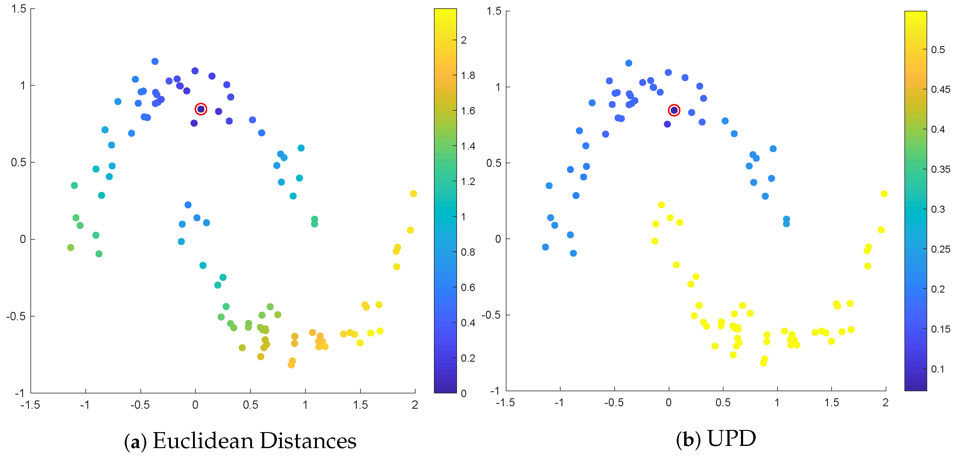
Intuitively, UPD computes the maximal edge length in each path, then minimizes this quantity over all paths. It may be understood as an -geodesic, while the classical shortest path is the -geodesic. Two points are far apart in the UPD if every path between them has at least one large edge. Compared to the geodesic, which is density-agnostic, the UPD prefers paths that avoid low-density regions. Like classical shortest paths, it may be computed efficiently using a Dijkstra-type algorithm [35]. A comparison of Euclidean distances and UPD is in Figure 1.
For clustering data generated from mixtures of manifolds, the UPD is extremely robust to diffuse background noise (e.g., uniformly sampled background points), and enjoys excellent performance guarantees for distinguishing between points in the same and different clusters [12]. Indeed, UPD have the property that for separated clusters with sufficiently many points, is uniformly small when lie in the same cluster and uniformly large when x and y lie in distinct clusters. This holds even for high-dimensional data, as long as the underlying clusters are low-dimensional (e.g., localize near noisy subspaces or Riemannian manifolds) and background noise does not concentrate in high density regions. These desirable properties are not held by classical metrics such as Euclidean distances, and suggest the utility of UPD for HSI clustering. In particular, we propose to leverage the desirable properties of UPD by incorporating it into the spectral clustering algorithm.
We remark that UPD are not universally appropriate as a metric for clustering, and in particular will fail to distinguish overlapping clusters that are generated by sampling uniformly (i.e., the overlapping clusters with approximately constant density). However, overlapping clusters in which the overlapping regions are low-density are suitable for UPD [36], for example overlapping Gaussian clusters.
2.3. Background on Spectral Clustering
Spectral clustering uses low-frequency eigenfunctions of a graph Laplacian as new coordinates for high-dimensional, nonlinear data, on which a traditional clustering algorithm can be run (e.g., K-means or Gaussian mixture models) [37]. For data and metric , define a weighted, undirected graph with nodes X and weighted edges . The scaling parameter can be tuned manually, or set automatically [38]. Intuitively, there will be a strong edge between in if and only if is small relative to .
A natural approach to clustering is to partition into K communities that are internally large and well-connected and externally weakly connected. This may be formulated precisely in terms of the normalized cuts functional, which leads to an NP-hard computational problem [16]. This graph cut problem may be relaxed by considering eigenvectors of the graph Laplacian, which determine natural clusters in in polynomial time [8,16]. Indeed, let D be the diagonal degree matrix with . Let be the (symmetric normalized) graph Laplacian. Note is positive semi-definite, with a number of zero eigenvalues equal to the number of connected components in .
The spectral clustering algorithm (Algorithm 1) computes the lowest frequency eigenvectors of L (those with smallest eigenvalues) and uses them as features in K-means clustering [8]. Note that we formulate Algorithm 1 as taking only W and a number of clusters K as an input. In practice, W must be computed using some metric . While the Euclidean metric is common, other metrics may provide superior performance [12,39,40]. Indeed, the metric should be chosen so that points in the same cluster appear well-connected, while points in different clusters are well-separated [41]. Our approach recognizes that spatially-regularized UPD achieves this for high-dimensional, noisy HSI.
| Algorithm 1 Spectral Clustering (SC) |
| Input:W, K; Output:
|
3. Algorithm
The proposed SRUSC method (Algorithm 2) consists in performing spectral clustering using the UPD and a spatially regularized graph Laplacian. The use of makes points in the same cluster appear close together, as long as there is a high-density path connecting them, while pushing apart points in distinct clusters separated by a density gap. The spatial regularization accounts for the image structure of the HSI and the latent spatial smoothness of the labels on the HSI.
Mathematically, let
where is the set of all pixels in the full image whose spatial coordinates lie inside the square with side lengths r centered at . For points within spatial distance r of an image boundary, no periodic extension of the spatial square is applied; these points are simply connected to fewer points than interior points. The constraint that if or enforces spatial regularity in the graph: a pixel can only be connected to spatially proximal pixels. Spatial regularization has been shown to improve clustering performance for HSI, by producing clusters that are smoother with respect to the underlying spatial structure [24,34]. It also has a sparsifying effect, since W has only non-zero entries. This affords a substantial computational advantage in the subsequent eigenvector calculation when . Note also that outlier denoising may be performed as a pre-processing step, by removing any points whose nearest neighbor distance in exceeds a threshold . This accounts for high-dimensional outliers that are known to be problematic for spectral clustering [36]. The labels of these (typically very few) points are computed by a majority vote in a local spatial neighborhood at the final step. In some of our experiments, we found this a helpful pre-processing step. While not strictly necessary, we include this optional pre-processing step as part of Algorithm 2.
| Algorithm 2 Spatially Regularized Ultrametric SC (SRUSC), known |
| Input:); Output:
|
By connecting pixels with strong edges only if they are (i) spectrally close in UPD and (ii) spatially proximal, the resulting graph Laplacian detects communities corresponding to well-connected and spatially coherent clusters. This makes it well-suited to HSI, which often exhibit classes with those properties.
3.1. Discussion of Parameters
The parameters of Algorithm 2 are , and K, along with the optional denoising parameters . Spatially regularized spectral graph methods are typically robust to the choice of spatial radius r, and many automated methods exist for determining the scaling parameter in spectral clustering [38]. Theoretically, the denoising is highly robust to the choice of k and T, because there is a clear gap between inliers and outliers when using [12]. In practice on the datasets for which we denoised, we set and the voting radius to be as small as possible while maintaining that at least 10 non-denoised points are in each ball.
Estimation of K
On the other hand, the number of clusters K is notoriously challenging to estimate, particularly for data with nonlinear or elongated shapes. A commonly employed heuristic in spectral clustering is the eigengap heuristic, which estimates . However, this depends strongly on the scaling parameter used to construct the underlying graph. One can instead consider a multiscale eigengap [12,42], which simultaneously maximizes over the eigenvalue index and over :
where is a predetermined range of scaling parameter values, is an upper bound on the number of clusters, and is the -largest eigenvalue of the graph Laplacian L when it is computed using a weight matrix W with scaling parameter . The estimated optimal parameters are chosen to maximize this multiscale eigengap by varying over k and simultaneously. This yields a nearly totally unsupervised algorithm, in which the user need only specify the spatial radius r, a range S of candidate values, and an upper bound on the number of clusters . Making the choices suggested above, this nearly parameter-free algorithm is summarized in Algorithm 3.
| Algorithm 3 Spatially Regularized Ultrametric SC (SRUSC), unknown |
| Input:; Output:
|
Computationally, Algorithm 3 loops over the elements of S, and is therefore slower than Algorithm 2. However, under the very reasonable assumptions that with respect to n (i.e., the number of candidate scaling parameters does not increase with n) and that with respect to n (i.e., the number of clusters is constant with respect to n) the computational complexity of Algorithm 3 is still quasilinear in n. In practice, we set for all experiments and S to be 20 equally spaced points covering the range of -distances in the data.
3.2. Computational Complexity
A benefit of the proposed method is that when r is small and the number of clusters K does not grow with n, Algorithm 2 (and similarly Algorithm 3) is fast, as quantified in the following theorem.
Theorem 1.
The computational complexity of Algorithm 2 is .
Proof.
Note that the graph Laplacian L constructed in the proposed method is -sparse. Since the cost of computing is proportional to the number of edges in the underlying graph , the complexity of computing L is , where k is the number of nearest neighbors in . It is known that is sufficient to ensure that with high probability the UPD on a k-nearest neighbors graph and UPD on the fully connected graph are the same [12,43]. For such a k, the computation of L is . Once L is computed, getting the lowest frequency eigenvectors is using iterative methods [44]. Finally, running K-means via Lloyd’s algorithm on these eigenvectors is when the number of iterations is constant with respect to n. This gives an overall complexity of
□
This scaling is essentially optimal with respect to n, since loading the underlying data into memory already has complexity . Note, however, that sparsity of the underlying matrix L is necessary to achieve quasilinear scaling. In particular, if r is too large, then SRUSC may not scale to large data sets. We remark that the quasilinear scaling of SRUSC matches the quasilinear scaling achieved by traditional spectral clustering on sparse graphs.
4. Experimental Analysis
To validate the proposed method, we perform clustering experiments on five data sets: three synthetic HSI and two real HSI.
The first synthetic data set is denoted “Four Spheres" (FS), and is generated as follows. Consider four centers in , , and , and a fixed radius 1.7. To generate a synthetic pixel associated to one of these centers, 99 samples are generated from the corresponding sphere with the given center and radius , generated uniformly at random from . These 99 samples are concatenated to form a vector in , with uniform samples from used to pad and create a vector in . We generate 4900 points associated to each center in this way. There are 2 clusters: the union of points associated to the centers and ; and the points associated to the center . The idea is that each of the four centers generate samples that are separable by a nonlinear boundary, but the fourth center is substantially further from the first three. Thus, the most natural number of clusters is 2. It is expected that this data set will be challenging due to the nonlinear cluster boundaries, lack of separability in the last two coordinates, and large within-cluster variances. Each of the 4 groups of 4900 points are spatially arrayed to be , then are concatenated spatially into a synthetic HSI; see Figure 2.
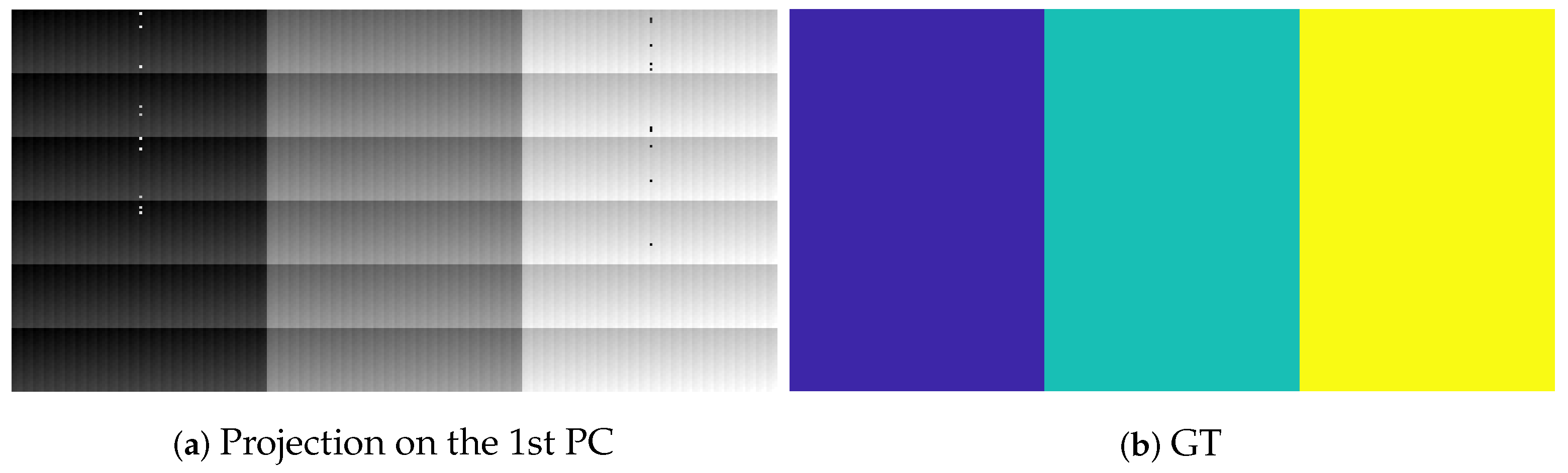
The second synthetic data set is denoted “Three Cubes” (TC) and consists of three clusters, generated as follows. Vectors are sampled uniformly from , then padded with zeros to make vectors in . These points are then concatenated and rotated by an orthogonal matrix sampled uniformly at random by performing a QR-decomposition on a random Gaussian matrix. The data is then embedded in by padding all the data with 0 in the 200th coordinate. Finally, the second cluster is translated by and the third cluster by . In this sense, the clusters are intrinsically 3-dimensional cubes, embedded and separated in a high-dimensional ambient space [45]. Each cube contains 13824 points, spatially arrayed to be . These clusters are concatenated spatially into a synthetic HSI; see Figure 3. To demonstrate the necessity of spatial regularization, we randomly select 30 points from the middles of cluster 1 and cluster 3 and swap them. This can be understood as adversarial noise, to which we expect spatially regularized methods to be robust. This presupposes a kind of spatial regularity in this synthetic image that is often, but not always, reasonable for real data (e.g., it may be reasonable for HSI of natural scenes, but not urban ones).
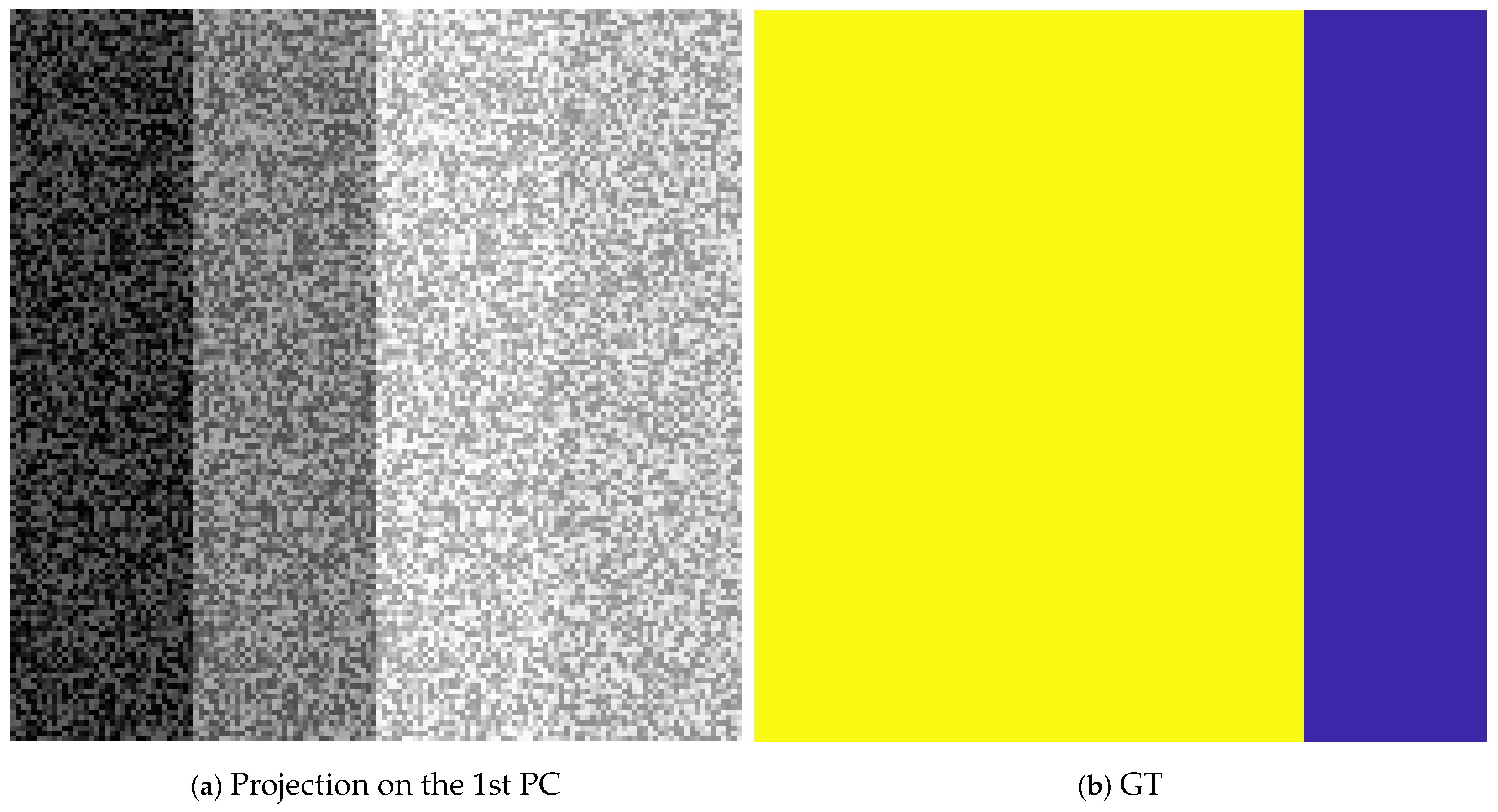
The third synthetic data set is generated by sampling 5000 data points from 10 different overlapping Gaussians in , each with different mean and the same covariance matrix. The means for ten Gaussian are of the form , where with common covariance matrix . The 5-dimensional data are then padded with 0s to create data in , then rotated by a random orthogonal matrix, similar to the FS data. We label each point according to which Gaussian mean it is nearest; this accounts for the overlap in the Gaussians. The synthetic spectral data data is then arranged so that the first rectangle of synthetic spectra are sampled from the first Gaussian, the second rectangle are sampled from the second Gaussian, and so on. Therefore, the size of the data is and each class has 500 pixels; see Figure 4.
We also consider two real HSI data sets: the Salinas A and Pavia U data sets (http://www.ehu.eus/ccwintco/index.php/Hyperspectral_Remote_Sensing_Scenes, accessed on 1 August 2019). Visualizations of the real HSI, along with their partial ground truth, are in Figure 5 and Figure 6, respectively. Note that both of these data sets contain a relatively small number of classes; in the case of Pavia U we chose to crop a small subregion to use for experiments, due to both the well-documented challenges of using too many ground truth classes for unsupervised HSI clustering of real data [46], and in order to ensure that most pixels in the image had ground truth labels.
4.1. Comparison Methods
We compare with four benchmark clustering methods, as well as five state-of-the-art methods. The four benchmark methods are:
The five state-of-the-art methods are:
- Density Peaks Clustering (DPC) (https://people.sissa.it/~laio/Research/Res_clustering.php, accessed on 1 January 2020) [15];
- Hierarchical Nonnegative Matrix Factorization (NMF) (https://sites.google.com/site/nicolasgillis/code, accessed on 1 January 2017) [22];
- Laplacian-Regularized Low-Rank Subspace Clustering (LLRSC) [20];
- Local Covariance Matrix Representation (LCMR) (https://github.com/henanjun/LCMR, accessed on 1 January 2020) [49]
The DL and NMF methods have, in particular, shown excellent performance on HSI while enjoying a high degree of theoretical interpretability. In Section 4.2, we assume the number of clusters K is known a priori. In Section 4.4, we show how the proposed method can estimate K.
We note the LCMR method is a supervised learning algorithm. After dimension reduction, the algorithm uses the cosine distance to compute the local neighboring data points, and applies the covariance matrix representation to each data point. Finally, an SVM uses the covariance matrices as the inputs to label the images. The algorithm uses a number of training labels equal to , where as always K is the number of classes in the ground truth. The purpose of including this supervised method amongst the unsupervised comparison methods is to demonstrate the effectiveness of SRUSC even compared to supervised ones which have access to labeled training data.
4.2. Clustering Accuracy
To perform quantitative comparisons, we align each clustered data set with the ground truth by solving a linear assignment problem with the Hungarian algorithm [50]. Then, three accuracy measures are computed: overall accuracy (ratio of correctly labeled pixels to total number of pixels), denoted OA; average accuracy (the average OA on each class), denoted AA; and Cohen’s statistic [51]. Numerical results are in Table 1, with visual results in Figure 7, Figure 8, Figure 9, Figure 10 and Figure 11. Note that the accuracy metrics are only computed on pixels that have ground truth labels. Moreover, the alignments were made to maximize OA, and different alignments may be realized if AA or are maximized.
We see that across all datasets, SRUSC outperforms all comparison methods. While many methods perform well on the synthetic data, only SRUSC performs well on both of the real data sets as well. Generally, SC and DL perform second best, which makes sense since they are also graph-based methods. Remarkably, the proposed method even outperforms the supervised LCMR method, which makes use of labeled training data to predict.
4.3. Discussion of Tunable Parameters
There are three major parameters to tune for the proposed method (Algorithm 3): . The spatial radius r needs to be chosen large enough to capture important spatial patterns in the data, but not so large that many spatially disparate pixels in the image are connected. We found many choices of r were suitable for each data set, and that this was not a parameter to which SRUSC was extremely sensitive. The range of values, S, should be chosen to cover the range of values at a relatively fine sampling rate. We found taking 20 equally sized steps between the minimal and maximal -values worked well on all examples. Note that the larger is, the slower the proposed method. Similarly, we found taking allowed for efficient detection of K. Taking it larger would needlessly increase runtime by requiring more eigenvalues to be computed at each . We note that no denoising was done on the Four Spheres and Three Cubes synthetic data, while pre-processing denoising on the Ten Gaussians (), Salinas A (), and Pavia U () was performed. These cutoffs were performed by visual inspection, noting that in all cases there was a clear gap between noisy outliers and inlying cluster points.
4.4. Estimation of Number of Clusters
While clustering accuracy when given K a priori is an important metric for clustering algorithm evaluation, it is not entirely realistic. Indeed, the estimation of K is an important yet poorly understood problem not just in HSI clustering, but in clustering more generally.
In Figure 12, the eigenvalues of the SRUSC Laplacian are shown for a range of scales . We see the eigengap (3) correctly estimates number of clusters for most of the data sets considered, for a range of values. Only on Salinas A does the eigengap fail; it estimates 7 rather than 6 clusters. We note, however, that in this case one of the classes (in the bottom right) is obviously spectrally separable into two distinct regions. Since the algorithm is provided only with the unlabeled data, returning 7 as the number of clusters is arguably more reasonable than returning 6, the latter being the number of ground truth classes. Indeed, it is essentially impossible to link the split class based on the spectral data alone—supervision is required.
Overall, these results suggest that SRUSC is able to estimate (exactly or nearly) the number of clusters even on challenging, high-dimensional HSI.
Note that we also estimated the number of clusters using multiscale eigenvalues computed with the Euclidean Laplacian, with very poor results; see Figure 12f–j. Indeed, the Euclidean multiscale eigenvalues fail to reasonably estimate K in any of the examples considered. This suggests another important advantage of SRUSC compared to more classical graph-based clustering methods: it can estimate the number of clusters, making it nearly completely unsupervised.
4.5. Runtime
The runtimes for all algorithms are in Table 2. All experiments were performed on a Macbook Pro with a 3.5GHz Intel Core i7 processor and 16GB RAM. We see that the graph-based methods (SC, DL, SRUSC) are on a similar order of magnitude, and are considerably slower than simpler and less effective methods like KM and GMM.
5. Conclusions and Future Research
In this article, we showed that UPD are a powerful and efficient metric for the unsupervised analysis of HSI. When embedded in the spectral clustering framework and combined with suitable spatial regularization, state-of-the-art clustering performance is realized by the SRUSC algorithm on a range of synthetic and real data sets. Moreover, ultrametric spectral clustering is mathematically rigorous and enjoys theoretical understanding of its accuracy and robustness to parameters that many unsupervised learning algorithms lack.
Based on the success of unsupervised learning with ultrametric path distances, it is of interest to develop semisupervised UPD approaches for HSI. Path distances for semisupervised learning are effective in several contexts [52], and it is of interest to understand how the UPD perform in the context of high-dimensional HSI, specifically for active learning of HSI [53,54].
A related line of work is to regularize the geodesic not through spatial regularization, but through the addition of another metric (i.e., geodesic or Euclidean distance). This would have the effect of requiring the optimizing path in the HSI pixel space to be short in multiple sense, and is expected to improve robustness. For both this form of regularization and the spatial regularization proposed in this article, it is of interest to develop mathematical clustering performance guarantees depending on, for example, the joint spectral-spatial smoothness of the HSI.
It is also of interest to develop hierarchical clustering methods based on UPD, which will mitigate the challenge of using incompletely-labeled ground truth data to do algorithmic validation. Indeed, allowing for soft clusterings and multiscale labelings is closer to the practical use-case of HSI clustering algorithms, in which remote sensing scientists need to explore real data for which they have little or no knowledge of the underlying material classes. Developing methods and intrinsic clustering evaluation metrics (that do not require labeled ground truth) are the topic of ongoing research. A related line of inquiry pertains to intrinsic statistics that measure whether or not to split clusters or preserve them [55]. It is of interest to apply both classical methods (e.g., silhouette scores [56] and the Davies–Bouldin index (DBI) [57]) and also recent methods based on diffusion processes [58] to evaluate intrinsic cluster structure in the context of SRUSC. Indeed, balancing cohesion within and separation between clusters is an important underlying principle for clustering that will be explored via hierarchical methods.
Author Contributions
J.M.M. conceived the project. S.Z. ran all experiments. S.Z. and J.M.M. wrote the manuscript. All authors have read and agreed to the published version of the manuscript.
Funding
This research is partially supported by the US National Science Foundation grants NSF-DMS 1912737, NSF-DMS 1924513, and NSF-CCF 1934553.
Informed Consent Statement
Not applicable.
Data Availability Statement
All code is publicly available at https://github.com/ShukunZhang/Spatially-Regularized-Ultrametrics (accessed on 2 October 2020).
Conflicts of Interest
The authors declare no conflict of interest.
References
- Melgani, F.; Bruzzone, L. Classification of hyperspectral remote sensing images with support vector machines. IEEE Trans. Geosci. Remote Sens. 2004, 42, 1778–1790. [Google Scholar] [CrossRef] [Green Version]
- Camps-Valls, G.; Gomez-Chova, L.; Muñoz-Marí, J.; Vila-Francés, J.; Calpe-Maravilla, J. Composite kernels for hyperspectral image classification. IEEE Geosci. Remote Sens. Lett. 2006, 3, 93–97. [Google Scholar] [CrossRef]
- Tarabalka, Y.; Fauvel, M.; Chanussot, J.; Benediktsson, J. SVM-and MRF-based method for accurate classification of hyperspectral images. IEEE Geosci. Remote Sens. Lett. 2010, 7, 736–740. [Google Scholar] [CrossRef] [Green Version]
- Chen, Y.; Lin, Z.; Zhao, X.; Wang, G.; Gu, Y. Deep learning-based classification of hyperspectral data. IEEE J. Select. Top. Appl. Earth Obs. Remote Sens. 2014, 7, 2094–2107. [Google Scholar] [CrossRef]
- Zhao, W.; Du, S. Spectral–spatial feature extraction for hyperspectral image classification: A dimension reduction and deep learning approach. IEEE Trans. Geosci. Remote Sens. 2016, 54, 4544–4554. [Google Scholar] [CrossRef]
- Li, S.; Song, W.; Fang, L.; Chen, Y.; Ghamisi, P.; Benediktsson, J. Deep learning for hyperspectral image classification: An overview. IEEE Trans. Geosci. Remote Sens. 2019, 57, 6690–6709. [Google Scholar] [CrossRef] [Green Version]
- Friedman, J.; Hastie, T.; Tibshirani, R. The Elements of Statistical Learning; Springer Series in Statistics; Springer: Berlin, Germany, 2001; Volume 1. [Google Scholar]
- Ng, A.; Jordan, M.; Weiss, Y. On spectral clustering: Analysis and an algorithm. In Advances in Neural Information Processing Systems; MIT: Cambridge, MA, USA, 2001; Volume 14, pp. 849–856. [Google Scholar]
- Baldi, P. Autoencoders, unsupervised learning, and deep architectures. In Proceedings of ICML Workshop on Unsupervised and Transfer Learning; JMLR Workshop and Conference Proceedings: Edinburgh, Scotland, 2012; pp. 37–49. [Google Scholar]
- Song, C.; Liu, F.; Huang, Y.; Wang, L.; Tan, T. Auto-encoder based data clustering. In Iberoamerican Congress on Pattern Recognition; Springer: Berlin, Germany, 2013; pp. 117–124. [Google Scholar]
- Haeffele, B.; You, C.; Vidal, R. A critique of self-expressive deep subspace clustering. arXiv 2020, arXiv:2010.03697. [Google Scholar]
- Little, A.; Maggioni, M.; Murphy, J. Path-Based Spectral Clustering: Guarantees, Robustness to Outliers, and Fast Algorithms. J. Mach. Learn. Res. 2020, 21, 1–66. [Google Scholar]
- Le Moan, S.; Cariou, C. Minimax Bridgeness-Based Clustering for Hyperspectral Data. Remote Sens. 2020, 12, 1162. [Google Scholar] [CrossRef] [Green Version]
- Ester, M.; Kriegel, H.; Sander, J.; Xu, X. A density-based algorithm for discovering clusters in large spatial databases with noise. In Kdd; AAAI: New Orleans, LA, USA, 1996; Volume 96, pp. 226–231. [Google Scholar]
- Rodriguez, A.; Laio, A. Clustering by fast search and find of density peaks. Science 2014, 344, 1492–1496. [Google Scholar] [CrossRef] [Green Version]
- Shi, J.; Malik, J. Normalized cuts and image segmentation. IEEE Trans. Pattern Anal. Mach. Intell. 2000, 22, 888–905. [Google Scholar]
- Bachmann, C.; Ainsworth, T.; Fusina, R. Exploiting manifold geometry in hyperspectral imagery. IEEE Trans. Geosci. Remote Sens. 2005, 43, 441–454. [Google Scholar] [CrossRef]
- Lunga, D.; Prasad, S.; Crawford, M.; Ersoy, O. Manifold-learning-based feature extraction for classification of hyperspectral data: A review of advances in manifold learning. IEEE Signal Proc. Mag. 2013, 31, 55–66. [Google Scholar] [CrossRef]
- Zhang, H.; Zhai, H.; Zhang, L.; Li, P. Spectral–spatial sparse subspace clustering for hyperspectral remote sensing images. IEEE Trans. Geosci. Remote Sens. 2016, 54, 3672–3684. [Google Scholar] [CrossRef]
- Zhai, H.; Zhang, H.; Zhang, L.; Li, P. Laplacian-regularized low-rank subspace clustering for hyperspectral image band selection. IEEE Trans. Geosci. Remote Sens. 2018, 57, 1723–1740. [Google Scholar] [CrossRef]
- Chen, Z.; Zhang, C.; Mu, T.; Yan, T.; Chen, Z.; Wang, Y. An Efficient Representation-Based Subspace Clustering Framework for Polarized Hyperspectral Images. Remote Sens. 2019, 11, 1513. [Google Scholar] [CrossRef] [Green Version]
- Gillis, N.; Kuang, D.; Park, H. Hierarchical clustering of hyperspectral images using rank-two nonnegative matrix factorization. IEEE Trans. Geosci. Remote Sens. 2015, 53, 2066–2078. [Google Scholar] [CrossRef] [Green Version]
- Zhang, L.; Zhang, L.; Du, B.; You, J.; Tao, D. Hyperspectral image unsupervised classification by robust manifold matrix factorization. Inf. Sci. 2019, 485, 154–169. [Google Scholar] [CrossRef]
- Cahill, N.; Czaja, W.; Messinger, D. Schroedinger eigenmaps with nondiagonal potentials for spatial-spectral clustering of hyperspectral imagery. In Algorithms and Technologies for Multispectral, Hyperspectral, and Ultraspectral Imagery XX; International Society for Optics and Photonics: Bellingham, DC, USA, 2014; Volume 9088, p. 908804. [Google Scholar]
- Zhao, Y.; Yuan, Y.; Wang, Q. Fast spectral clustering for unsupervised hyperspectral image classification. Remote Sens. 2019, 11, 399. [Google Scholar] [CrossRef] [Green Version]
- Wang, R.; Nie, F.; Wang, Z.; He, F.; Li, X. Scalable graph-based clustering with nonnegative relaxation for large hyperspectral image. IEEE Trans. Geosci. Remote Sens. 2019, 57, 7352–7364. [Google Scholar] [CrossRef]
- Murphy, J.; Maggioni, M. Unsupervised Clustering and Active Learning of Hyperspectral Images with Nonlinear Diffusion. IEEE Trans. Geosci. Remote Sens. 2019, 57, 1829–1845. [Google Scholar] [CrossRef] [Green Version]
- Qin, Y.; Bruzzone, L.; Li, B. Learning discriminative embedding for hyperspectral image clustering based on set-to-set and sample-to-sample distances. IEEE Trans. Geosci. Remote Sens. 2019, 58, 473–485. [Google Scholar] [CrossRef]
- Sellami, A.; Abbes, A.; Barra, V.; Farah, I. Fused 3-D spectral-spatial deep neural networks and spectral clustering for hyperspectral image classification. Pattern Recogn. Lett. 2020, 138, 594–600. [Google Scholar] [CrossRef]
- Zhang, Y.; Du, B.; Zhang, L.; Wang, S. A low-rank and sparse matrix decomposition-based Mahalanobis distance method for hyperspectral anomaly detection. IEEE Trans. Geosci. Remote Sens. 2015, 54, 1376–1389. [Google Scholar] [CrossRef]
- Xu, Y.; Wu, Z.; Chanussot, J.; Wei, Z. Joint reconstruction and anomaly detection from compressive hyperspectral images using Mahalanobis distance-regularized tensor RPCA. IEEE Trans. Geosci. Remote Sens. 2018, 56, 2919–2930. [Google Scholar] [CrossRef]
- Heylen, R.; Scheunders, P. A distance geometric framework for nonlinear hyperspectral unmixing. IEEE J. Select. Top. Appl. Earth Obs. Remote Sens. 2014, 7, 1879–1888. [Google Scholar] [CrossRef]
- Wang, R.; Nie, F.; Yu, W. Fast spectral clustering with anchor graph for large hyperspectral images. IEEE Geosci. Remote Sens. Lett. 2017, 14, 2003–2007. [Google Scholar] [CrossRef]
- Murphy, J.; Maggioni, M. Spectral-spatial diffusion geometry for hyperspectral image clustering. IEEE Geosci. Remote Sens. Lett. 2020, 17, 1243–1247. [Google Scholar] [CrossRef] [Green Version]
- McKenzie, D.; Damelin, S. Power weighted shortest paths for clustering Euclidean data. Found. Data Sci. 2019, 1, 307. [Google Scholar] [CrossRef] [Green Version]
- Arias-Castro, E. Clustering based on pairwise distances when the data is of mixed dimensions. IEEE Trans. Inf. Theory 2011, 57, 1692–1706. [Google Scholar] [CrossRef] [Green Version]
- Von Luxburg, U. A tutorial on spectral clustering. Stat. Comput. 2007, 17, 395–416. [Google Scholar] [CrossRef]
- Zelnik-Manor, L.; Perona, P. Self-tuning spectral clustering. In Advances in Neural Information Processing Systems; MIT: Cambridge, MA, USA, 2005; pp. 1601–1608. [Google Scholar]
- Elhamifar, E.; Vidal, R. Sparse manifold clustering and embedding. In Advances in Neural Information Processing Systems; MIT: Cambridge, MA, USA, 2011; pp. 55–63. [Google Scholar]
- Arias-Castro, E.; Lerman, G.; Zhang, T. Spectral clustering based on local PCA. The J. Mach. Learn. Res. 2017, 18, 253–309. [Google Scholar]
- Schiebinger, G.; Wainwright, M.; Yu, B. The geometry of kernelized spectral clustering. Ann. Stat. 2015, 43, 819–846. [Google Scholar] [CrossRef] [Green Version]
- Little, A.; Byrd, A. A multiscale spectral method for learning number of clusters. In Proceedings of the 2015 IEEE 14th International Conference on Machine Learning and Applications (ICMLA), IEEE, Miami, FL, USA, 9–11 December 2015; pp. 457–460. [Google Scholar]
- González-Barrios, J.; Quiroz, A. A clustering procedure based on the comparison between the k nearest neighbors graph and the minimal spanning tree. Stat. Probab. Lett. 2003, 62, 23–34. [Google Scholar] [CrossRef]
- Trefethen, L.; Bau, D. Numerical Linear Algebra; Siam: Philadelphia, PA, USA, 1997; Volume 50. [Google Scholar]
- Elhamifar, E.; Vidal, R. Sparse subspace clustering: Algorithm, theory, and applications. IEEE Trans. Pattern Anal. Mach. Intell. 2013, 35, 2765–2781. [Google Scholar] [CrossRef] [PubMed] [Green Version]
- Zhu, W.; Chayes, V.; Tiard, A.; Sanchez, S.; Dahlberg, D.; Bertozzi, A.; Osher, S.; Zosso, D.; Kuang, D. Unsupervised classification in hyperspectral imagery with nonlocal total variation and primal-dual hybrid gradient algorithm. IEEE Trans. Geosci. Remote Sens. 2017, 55, 2786–2798. [Google Scholar] [CrossRef]
- Bishop, C. Pattern Recognition and Machine Learning; Springer: Berlin, Germany, 2006. [Google Scholar]
- Maggioni, M.; Murphy, J. Learning by Unsupervised Nonlinear Diffusion. J. Mach. Learn. Res. 2019, 20, 1–56. [Google Scholar]
- Fang, L.; He, N.; Li, S.; Plaza, A.; Plaza, J. A new spatial–spectral feature extraction method for hyperspectral images using local covariance matrix representation. IEEE Trans. Geosci. Remote Sens. 2018, 56, 3534–3546. [Google Scholar] [CrossRef]
- Munkres, J. Algorithms for the assignment and transportation problems. J. Soc. Ind. Appl. Math. 1957, 5, 32–38. [Google Scholar] [CrossRef] [Green Version]
- Banerjee, M.; Capozzoli, M.; McSweeney, L.; Sinha, D. Beyond kappa: A review of interrater agreement measures. Can. J. Stat. 1999, 27, 3–23. [Google Scholar] [CrossRef]
- Bijral, A.; Ratliff, N.; Srebro, N. Semi-supervised Learning with density based distances. In Proceedings of the Twenty-Seventh Conference on Uncertainty in Artificial Intelligence, Barcelona, Spain, 14–17 July 2011; pp. 43–50. [Google Scholar]
- Maggioni, M.; Murphy, J. Learning by Active Nonlinear Diffusion. Found. Data Sci. 2019, 1, 271–291. [Google Scholar] [CrossRef] [Green Version]
- Murphy, J. Spatially regularized active diffusion learning for high-dimensional images. Pattern Recogn. Lett. 2020, 135, 213–220. [Google Scholar] [CrossRef]
- Najafipour, S.; Hosseini, S.; Hua, W.; Kangavari, M.; Zhou, X. SoulMate: Short-text author linking through Multi-aspect temporal-textual embedding. IEEE Trans. Knowl. Data Eng. 2020. [Google Scholar] [CrossRef] [Green Version]
- Rousseeuw, P. Silhouettes: A graphical aid to the interpretation and validation of cluster analysis. J. Comput. Appl. Math. 1987, 20, 53–65. [Google Scholar] [CrossRef] [Green Version]
- Davies, D.; Bouldin, D. A cluster separation measure. IEEE Trans. Pattern Anal. Mach. Intell. 1979, 2, 224–227. [Google Scholar] [CrossRef]
- Murphy, J.; Polk, S. A Multiscale Environment for Learning by Diffusion. arXiv 2021, arXiv:2102.00500. [Google Scholar]
Figure 1.
The standard two moons dataset [8] is shown, with distances from a circled point shown in Euclidean distances (a) and UPD (b). We see that the UPD is much more effective at distinguishing between the two clusters. This is because there is a large density gap between the two clusters, while the density within each moon is roughly uniform. So, all the points in the top moon look close to the circled point, while all the points in the bottom moon look far.

Figure 2.
The four spheres synthetic data is and contains two clusters. The projection onto the first principal component is in (a), the ground truth labels in (b). A spatial radius of was used in SRUSC.
Figure 2.
The four spheres synthetic data is and contains two clusters. The projection onto the first principal component is in (a), the ground truth labels in (b). A spatial radius of was used in SRUSC.

Figure 3.
The three cubes synthetic data is and contains 3 clusters. The projection onto the first principal component is in (a), the ground truth labels in (b). A spatial radius of was used in SRUSC.
Figure 3.
The three cubes synthetic data is and contains 3 clusters. The projection onto the first principal component is in (a), the ground truth labels in (b). A spatial radius of was used in SRUSC.

Figure 4.
The ten Gaussian synthetic data is and contains 10 clusters. The projection onto the first principal component is in (a), the ground truth labels in (b). A spatial radius of was used in SRUSC.
Figure 4.
The ten Gaussian synthetic data is and contains 10 clusters. The projection onto the first principal component is in (a), the ground truth labels in (b). A spatial radius of was used in SRUSC.

Figure 5.
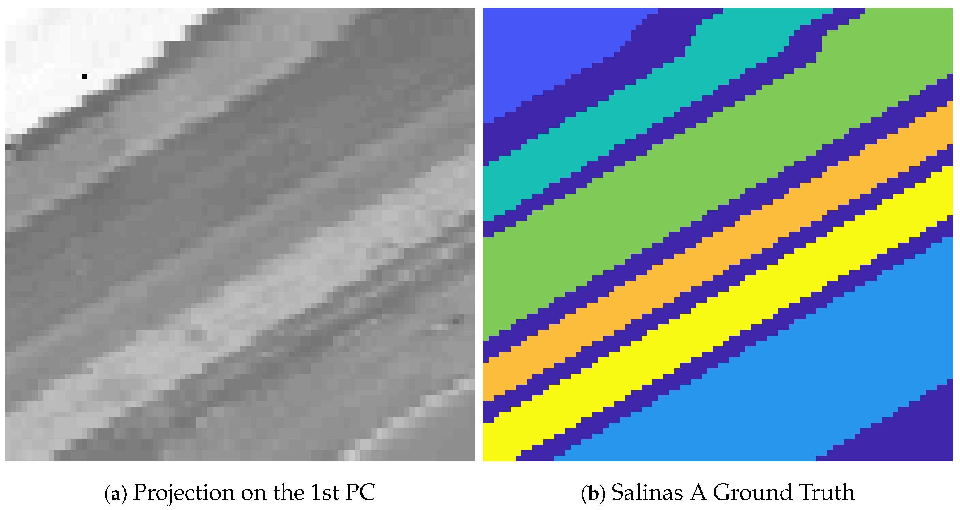
The Salinas A data set is a real HSI taken by the 224-band AVIRIS sensor over Salinas Valley, California. There are 6 clusters in the ground truth. The projection onto the first principal component is in (a), the ground truth labels in (b). A spatial radius of was used in SRUSC.
Figure 5.
The Salinas A data set is a real HSI taken by the 224-band AVIRIS sensor over Salinas Valley, California. There are 6 clusters in the ground truth. The projection onto the first principal component is in (a), the ground truth labels in (b). A spatial radius of was used in SRUSC.

Figure 6.
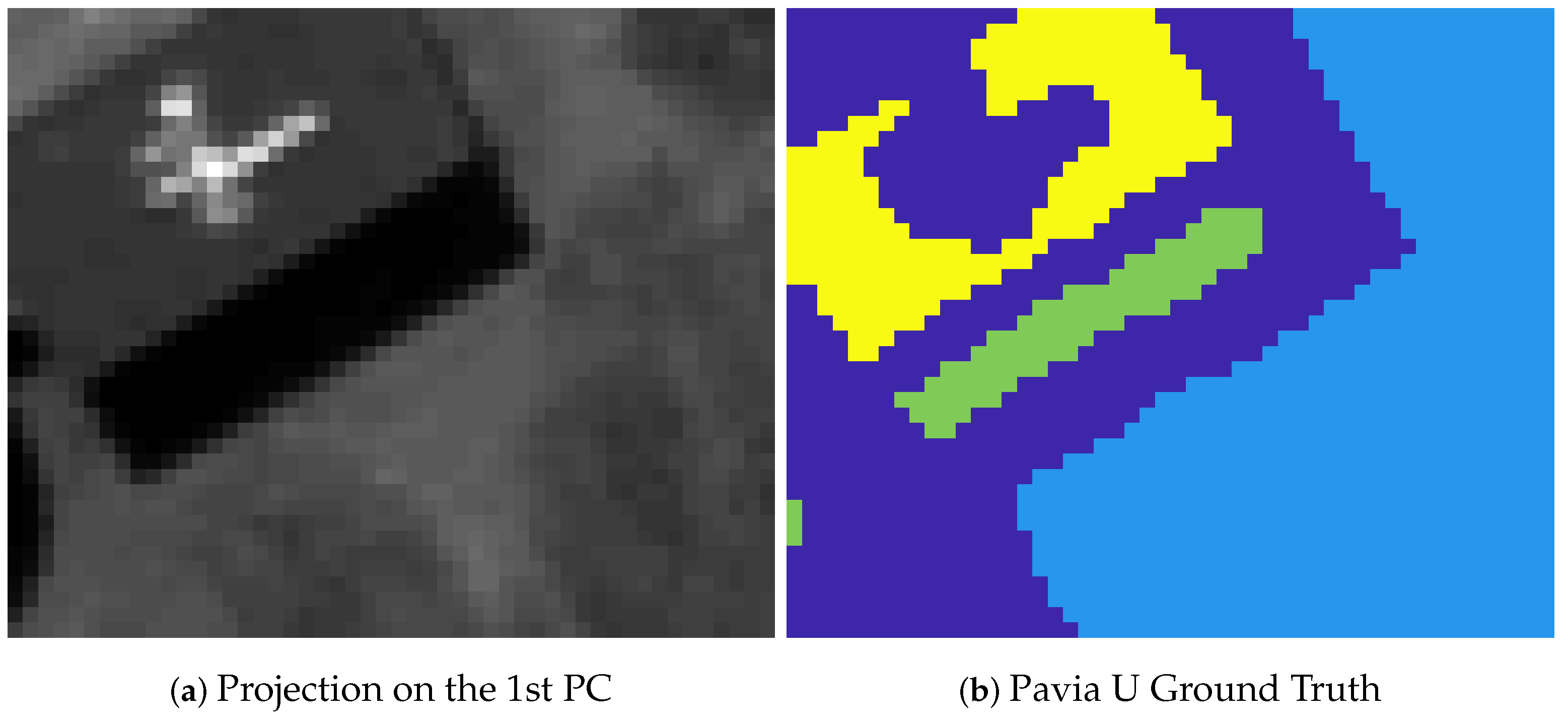
The Pavia U data set is a subset of the full HSI acquired by the 103-band ROSIS sensor over Pavia University. There are 3 clusters in the ground truth. The projection onto the first principal component is in (a), the ground truth labels in (b). A spatial radius of was used in SRUSC.
Figure 6.
The Pavia U data set is a subset of the full HSI acquired by the 103-band ROSIS sensor over Pavia University. There are 3 clusters in the ground truth. The projection onto the first principal component is in (a), the ground truth labels in (b). A spatial radius of was used in SRUSC.

Figure 7.
For the four spheres synthetic data set, several methods achieve perfect accuracy, including the proposed method. Interestingly, the proposed unsupervised SRUSC achieves perfect accuracy, while the supervised LCMR algorithm does not.
Figure 7.
For the four spheres synthetic data set, several methods achieve perfect accuracy, including the proposed method. Interestingly, the proposed unsupervised SRUSC achieves perfect accuracy, while the supervised LCMR algorithm does not.

Figure 8.
On the synthetic three cubes data set, only the proposed method is able to correctly label all data points. In particular, the spatial regularization is necessary to gain robustness to the noise introduced. Note, however, that the interpretation of the swapped points as noise relies on an assumption of spatial regularity in the pixel labels, which may not be reasonable in some contexts. While the swapped noise points were chosen randomly, repeated trials over which points were swapped did not change the numerical results significantly.

Figure 9.
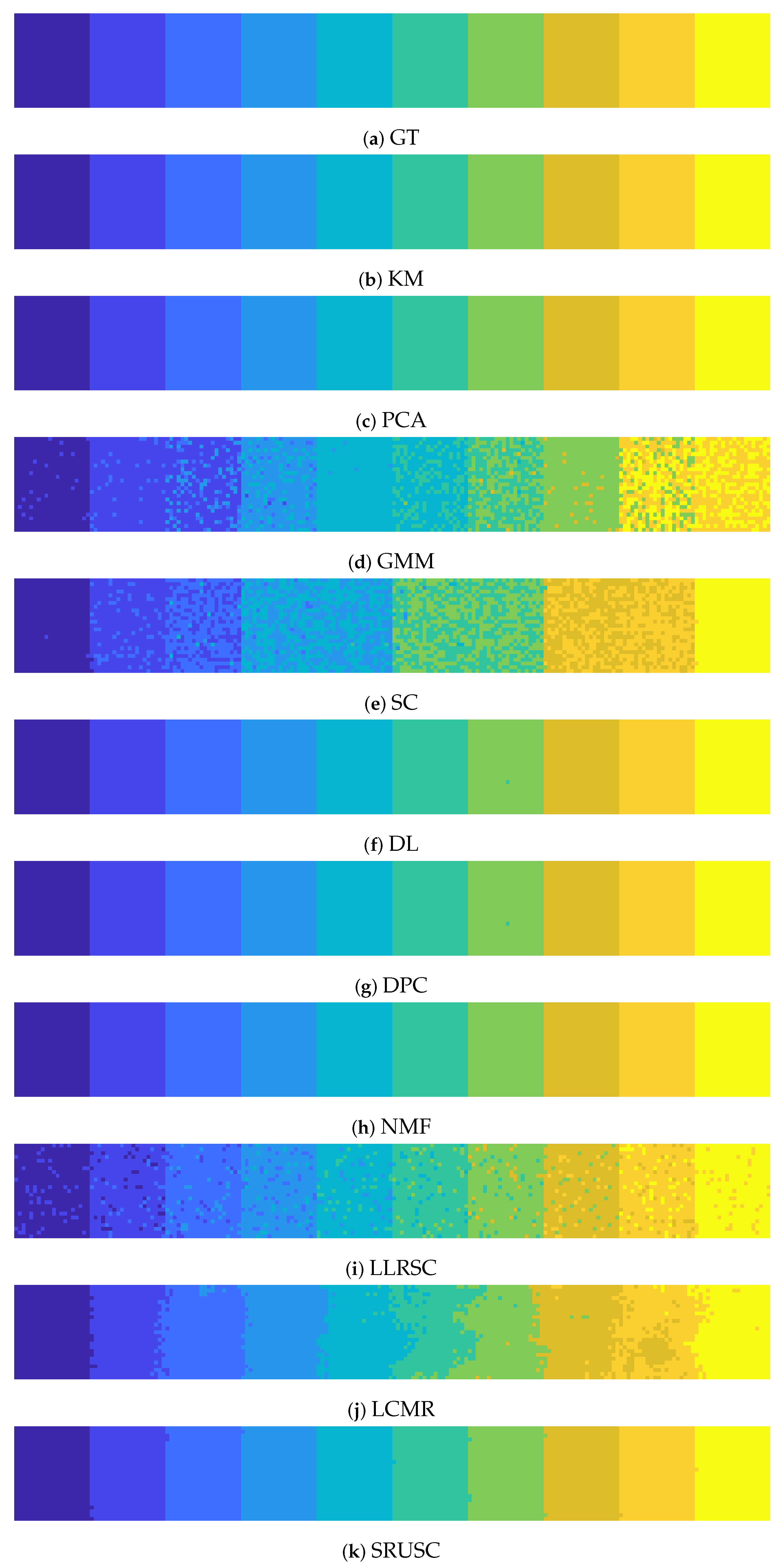
On the synthetic ten Gaussian data set, several models achieve nearly perfect accuracy, including the proposed method. However, both the SC and GMM methods fail to cluster properly. Note that our model only fails on a small number of points on the boundary of two different class, where the spatial information is not clear.
Figure 9.
On the synthetic ten Gaussian data set, several models achieve nearly perfect accuracy, including the proposed method. However, both the SC and GMM methods fail to cluster properly. Note that our model only fails on a small number of points on the boundary of two different class, where the spatial information is not clear.

Figure 10.
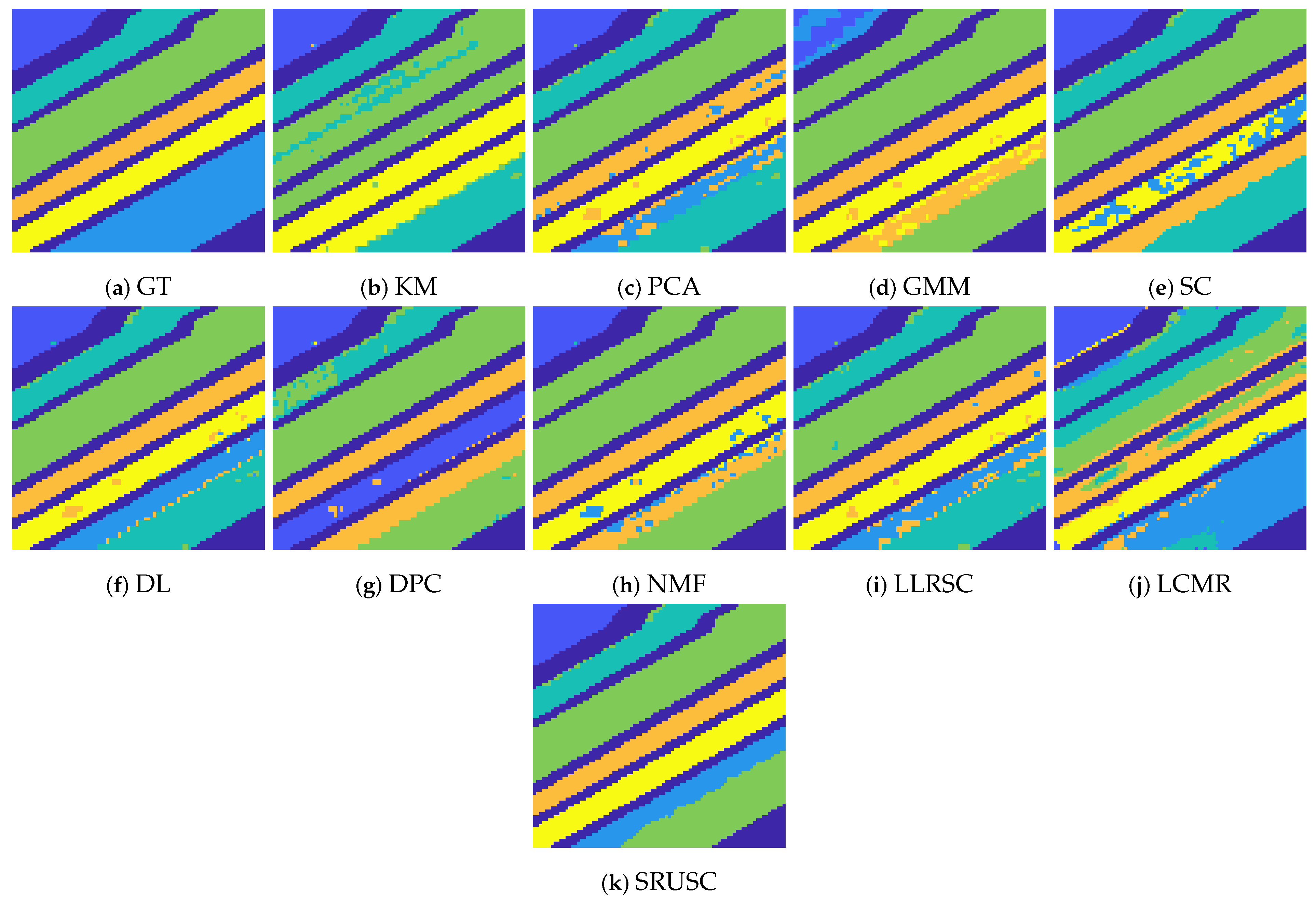
On the Salinas A data set, the proposed method performs strongly, with DL also performing well. Note that SRUSC nearly correctly estimates the number of clusters. As shown in Figure 12, it estimates 7 clusters rather than 6. This strong estimation is an additional advantage of SRUSC for the Salinas A dataset.
Figure 10.
On the Salinas A data set, the proposed method performs strongly, with DL also performing well. Note that SRUSC nearly correctly estimates the number of clusters. As shown in Figure 12, it estimates 7 clusters rather than 6. This strong estimation is an additional advantage of SRUSC for the Salinas A dataset.

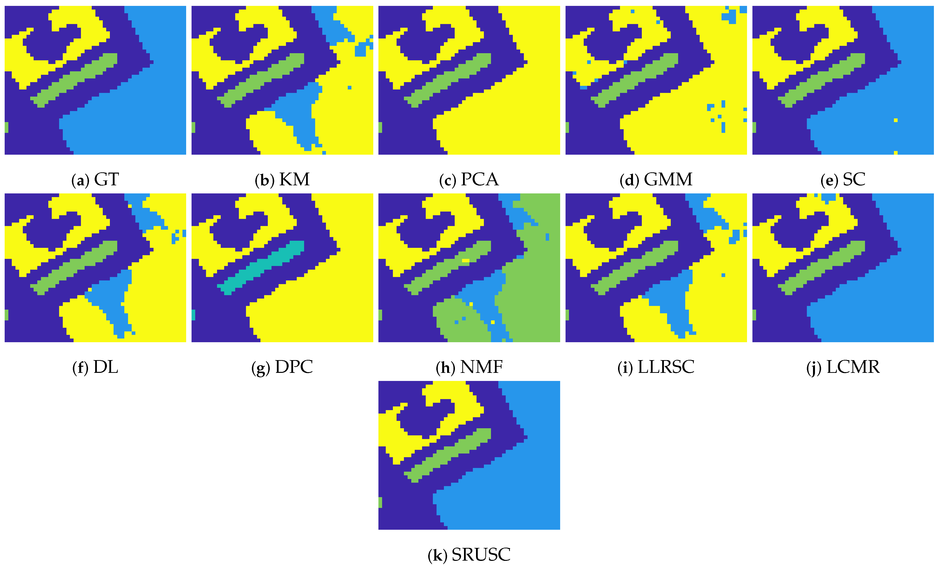
Figure 11.
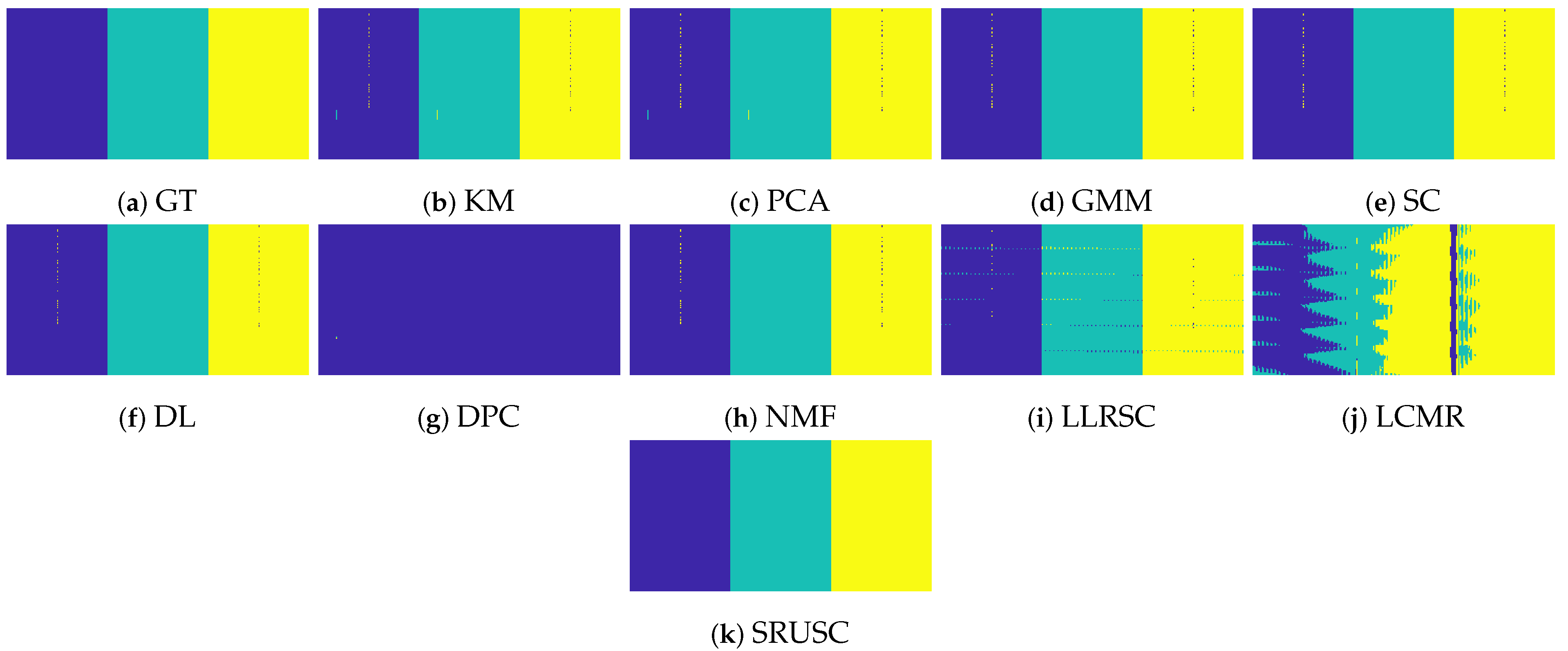
On the Pavia U data set, only the proposed method achieves perfect accuracy, though Euclidean spectral clustering and LCMR perform well. Moreover, SRUSC correctly estimates for this example; see Figure 12. This is a further advantage of SRUSC over SC (which fails to estimate K correctly) and LCMR (which is supervised).
Figure 11.
On the Pavia U data set, only the proposed method achieves perfect accuracy, though Euclidean spectral clustering and LCMR perform well. Moreover, SRUSC correctly estimates for this example; see Figure 12. This is a further advantage of SRUSC over SC (which fails to estimate K correctly) and LCMR (which is supervised).

Figure 12.
For each of the data sets, eigenvalues are shown as a function of . The ones on the top are the SRUSC eigenvalues (a–e), and on the bottom the Euclidean eigenvalues (f–j). The colors of the plots correspond to the eigenvalue index. The first eigenvalue is blue, and is always 0; the second eigenvalue is red, the third is yellow, the fourth is purple, the fifth is green, and so on. For a range of values, the largest gap for SRUSC is between the and eigenvalues for all three synthetic data sets, as well as Pavia U, indicating that SRUSC is correctly estimates K for these data. The proposed method estimates for Salinas A, rather than , which is perhaps a reasonable misestimation given the complexity of the data and the fact that one of the classes is spectrally incoherent. On the other hand, the Euclidean eigenvalues completely fail to correctly estimate K, even on the synthetic examples.


Table 1.
Results for clustering experiments. We see that across all methods and data sets, the proposed SRUSC method gives the best clustering performance.
Table 1.
Results for clustering experiments. We see that across all methods and data sets, the proposed SRUSC method gives the best clustering performance.
| Data Set | FS AA | TC AA | TG AA | SA AA | PU AA | FS OA | TC OA | TG OA | SA OA | PU OA | FS | TC | TG | SA | PU |
|---|---|---|---|---|---|---|---|---|---|---|---|---|---|---|---|
| KM | 1.00 | 1.00 | 1.00 | 0.66 | 0.58 | 1.00 | 1.00 | 1.00 | 0.63 | 0.60 | 1.00 | 1.00 | 1.00 | 0.53 | 0.09 |
| PCA | 1.00 | 1.00 | 1.00 | 0.85 | 0.67 | 1.00 | 1.00 | 1.00 | 0.80 | 0.79 | 1.00 | 1.00 | 1.00 | 0.76 | 0.39 |
| GMM | 0.51 | 1.00 | 0.62 | 0.58 | 0.80 | 0.56 | 1.00 | 0.62 | 0.59 | 0.57 | 0.51 | 1.00 | 0.58 | 0.48 | 0.36 |
| SC | 1.00 | 1.00 | 0.58 | 0.72 | 1.00 | 1.00 | 1.00 | 0.58 | 0.76 | 1.00 | 1.00 | 1.00 | 0.53 | 0.69 | 1.00 |
| DL | 0.77 | 1.00 | 1.00 | 0.88 | 0.38 | 0.66 | 1.00 | 1.00 | 0.83 | 0.60 | 0.77 | 1.00 | 1.00 | 0.79 | 0.07 |
| DPC | 0.77 | 0.33 | 1.00 | 0.61 | 0.34 | 0.66 | 0.33 | 1.00 | 0.63 | 0.65 | 0.77 | 0.33 | 1.00 | 0.54 | 0.03 |
| NMF | 0.94 | 1.00 | 1.00 | 0.67 | 0.59 | 0.90 | 1.00 | 1.00 | 0.64 | 0.76 | 0.94 | 1.00 | 1.00 | 0.54 | 0.52 |
| LLRSC | 0.75 | 1.00 | 0.86 | 0.75 | 0.67 | 0.62 | 1.00 | 0.86 | 0.77 | 0.79 | 0.75 | 1.00 | 0.85 | 0.75 | 0.67 |
| LCMR | 0.94 | 0.62 | 0.89 | 0.79 | 0.99 | 0.94 | 0.62 | 0.89 | 0.76 | 0.99 | 0.95 | 0.62 | 0.88 | 0.71 | 0.98 |
| SRUSC | 1.00 | 1.00 | 1.00 | 0.89 | 1.00 | 1.00 | 1.00 | 1.00 | 0.85 | 1.00 | 1.00 | 1.00 | 1.00 | 0.81 | 1.00 |
Table 2.
Running time for different methods measured in seconds. The methods that require the computation of eigenvectors of a graph (SC, DL, SRUSC) are slower than methods that do not. However, all methods require only at most minutes to run, even on the largest datasets.
Table 2.
Running time for different methods measured in seconds. The methods that require the computation of eigenvectors of a graph (SC, DL, SRUSC) are slower than methods that do not. However, all methods require only at most minutes to run, even on the largest datasets.
| Data Set | FS | TC | TG | SA | PU |
|---|---|---|---|---|---|
| KM | 0.7718 | 0.4352 | 0.1532 | 0.3206 | 0.1590 |
| PCA | 0.0472 | 0.0411 | 0.0372 | 0.0788 | 0.0479 |
| GMM | 3.4639 | 2.1814 | 0.6806 | 1.3530 | 0.1662 |
| SC | 563.8514 | 1832.7 | 9.3997 | 56.2373 | 2.0211 |
| DL | 870.0409 | 1036.8 | 23.7778 | 13.3009 | 1.2118 |
| DPC | 748.5418 | 1062.2 | 21.8215 | 9.6928 | 0.4860 |
| NMF | 0.4553 | 0.7978 | 0.6298 | 0.6593 | 0.3272 |
| LLRSC | 1.6171 | 1.0303 | 0.4702 | 1.15 | 0.4793 |
| LCMR | 240.5580 | 131.4040 | 4.55611 | 35.2812 | 3.5041 |
| SRUSC | 1402.1 | 2971.6 | 25.3597 | 97.4420 | 6.0195 |
Publisher’s Note: MDPI stays neutral with regard to jurisdictional claims in published maps and institutional affiliations. |
© 2021 by the authors. Licensee MDPI, Basel, Switzerland. This article is an open access article distributed under the terms and conditions of the Creative Commons Attribution (CC BY) license (http://creativecommons.org/licenses/by/4.0/).
Share and Cite
MDPI and ACS Style
Zhang, S.; Murphy, J.M. Hyperspectral Image Clustering with Spatially-Regularized Ultrametrics. Remote Sens. 2021, 13, 955. https://0-doi-org.brum.beds.ac.uk/10.3390/rs13050955
AMA Style
Zhang S, Murphy JM. Hyperspectral Image Clustering with Spatially-Regularized Ultrametrics. Remote Sensing. 2021; 13(5):955. https://0-doi-org.brum.beds.ac.uk/10.3390/rs13050955
Chicago/Turabian StyleZhang, Shukun, and James M. Murphy. 2021. "Hyperspectral Image Clustering with Spatially-Regularized Ultrametrics" Remote Sensing 13, no. 5: 955. https://0-doi-org.brum.beds.ac.uk/10.3390/rs13050955
Note that from the first issue of 2016, this journal uses article numbers instead of page numbers. See further details here.