
A Novel Approach to Estimating Time-Averaged Volcanic SO2 Fluxes from Infrared Satellite Measurements


1
Cooperative Institute for Meteorological Satellite Studies (CIMSS), University of Wisconsin-Madison, 1225 W. Dayton St., Madison, WI 53706, USA
2
Center for the Study of Active Volcanoes (CSAV), University of Hawai’i at Hilo, 200 W. Kawili Street, Hilo, HI 96720, USA
3
National Oceanic and Atmospheric Administration (NOAA), 1225 W. Dayton St., Madison, WI 53706, USA
*
Author to whom correspondence should be addressed.
Remote Sens. 2021, 13(5), 966; https://0-doi-org.brum.beds.ac.uk/10.3390/rs13050966
Submission received: 3 February 2021
/
Revised: 24 February 2021
/
Accepted: 27 February 2021
/
Published: 4 March 2021
(This article belongs to the Special Issue Quantitative Volcanic Hazard Assessment and Uncertainty Analysis in Satellite Remote Sensing and Modeling)
Abstract
:Long-term continuous time series of emissions are considered critical elements of both volcano monitoring and basic research into processes within magmatic systems. One highly successful framework for computing these fluxes involves reconstructing a representative time-averaged plume from which to estimate the source flux. Previous methods within this framework have used ancillary wind datasets from reanalysis or numerical weather prediction (NWP) to construct the mean plume and then again as a constrained parameter in the fitting. Additionally, traditional datasets from ultraviolet (UV) sensors lack altitude information, which must be assumed, to correctly calibrate the data and to capture the appropriate NWP wind level which can be a significant source of error. We have made novel modifications to this framework which do not rely on prior knowledge of the winds and therefore do not inherit errors associated with NWP winds. To perform the plume rotation, we modify a rudimentary computer vision algorithm designed for object detection in medical imaging to detect plume-like objects in gridded data. We then fit a solution to the general time-averaged dispersion of from a point source. We demonstrate these techniques using data generated by a newly developed probabilistic layer height and column loading algorithm designed for the Cross-track Infrared Sounder (CrIS), a hyperspectral infrared sensor aboard the Joint Polar Satellite System’s Suomi-NPP and NOAA-20 satellites. This data source is best suited to flux estimates at high-latitude volcanoes and at low-latitude, but high-altitude volcanoes. Of particular importance, IR data can fill an important data gap in the UV-based record: estimating emissions from high-latitude volcanoes through the polar winters when there is insufficient solar backscatter for UV sensors to be used.
1. Introduction
Many methods now exist to estimate volcanic sulfur dioxide () fluxes from satellite data. Over the last decade, much work has focused on long term, global monitoring of continuous low–moderate level volcanic emissions. These efforts are particularly useful for monitoring trends in volcanic activity as well as constraining the global volcanic flux for weather and climate studies. These methods for estimating long-term emission rates have relied on constructing and analyzing a time-averaged volcanic plume from satellite data generated by ultraviolet (UV) sensors. To do this, either the wind field advecting emissions must be remarkably stable e.g., [1] or the many plume observations in the averaging period must be rotated into a common wind field and then averaged together e.g., [2,3,4,5]. Once the time-averaged plume is constructed, a simplified plume dispersion model is fit to the time-averaged data. As described by [2], the measurement of flux is controlled by an estimate of the cloud mass and of the decay time which are estimated from the fitting results. Since the mean cloud mass is directly accessible from satellite measurements, the decay time (or lifetime) is the primary uncertain parameter.
Typically, numerical weather prediction (NWP) or re-analysis winds are used to analyze the wind direction to determine the rotation and then the wind speeds are used in the plume model fitting process. Errors in NWP, particularly in wind direction can have a significant effect on the reconstructed plume. In this process, a plume dispersal height must be assumed at which to capture the wind direction and speed and to estimate the vertical column density (VCD) itself. Typically, individual plume observations are assumed to have been advected by straight-line winds at one altitude; however, volcanic plumes are hot-sourced and can rise through many altitude levels each with its own wind speed and direction, resulting in the satellite observation of a distorted plume that may not be well-represented by an single local wind vector. These issues further complicate the use of wind data in reconstructing the time-averaged behavior.
Here we have made novel modifications in adopting this general approach which do not rely on prior knowledge of the winds and therefore do not inherit errors associated with NWP winds. In reconstructing the time-averaged plume, we exploit the geometry of the emitted clouds themselves to inform the wind-reconstruction. To perform the plume rotation, we modify a rudimentary computer vision algorithm designed for object detection in medical imaging to detect plume-like objects in gridded data. In light of the observation that many emissions of are offset from their sources along a different vector from their primary dispersal, we also allow short translations of the data so that these puffs can still be reconstructed in the case that there is a significant lag between emission and satellite overpass time.
In the fitting stage, we employ a solution to the general time-averaged dispersion of from a point source. This fitting function incorporates the time-averaged physics of decay, advection and turbulent mixing from a point source. This fitting function is more flexible than that employed by previous studies since it more closely approximates stream-wise eddy-diffusion mixing and is better suited to examining persistent point source emissions.
We demonstrate these techniques using data generated by a newly developed probabilistic layer height and VCD algorithm designed for the Cross-track Infrared Sounder (CrIS), a hyperspectral infrared (IR) sensor aboard the Joint Polar Satellite System (JPSS) series satellites: Suomi-NPP (SNPP) and NOAA-20 [6]. Since this algorithm retrieves the layer height, the retrieved VCD estimate is already calibrated for the appropriate altitude. This CrIS algorithm is currently integrated into the NOAA/CIMSS VOLcanic Cloud Analysis Toolkit VOLCAT; [7,8,9,10], where it is used to generate alerts as well as probabilistic cloud object properties for real-time detection, characterization, and tracking of volcanic clouds in support of aviation safety.
Although the use of hyperspectral IR data limits the accuracy of plume measurements in the lower troposphere, particularly in very moist tropical atmospheres, this data can still make useful flux estimates at high-latitude volcanoes and at low-latitude, but high-altitude volcanoes. Of particular importance, IR data can fill an important data gap in the UV-based record: estimating emissions from high-latitude volcanoes through the polar winters when there is insufficient solar backscatter for UV sensors due to the high solar zenith angle (SZA).
Our approach is modular, containing three main components: (1) the gridded data including a height estimate, (2) a wind-direction reconstruction algorithm to use in constructing time-averaged plumes, (3) an independent estimation of one of the sought geophysical parameters (here, decay rate or lifetime) and (4) a fitting model to estimate the plume shape and source flux. Consequently, these components are interchangeable with only minor adjustments which allows for customized application of this technique to suit the circumstances of measurement. Although we demonstrate this technique here with IR data, it is sufficiently general to be applied to UV measurements provided that an layer height can be reliably estimated. Additionally, these methods could be incorporated into a hybrid UV-IR technique such as changing from UV- to IR-based in the winter at high-latitude volcanoes.
1.1. Basic Principles of Time-Averaged SO Flux Estimation
As described above, similar techniques for estimating time-averaged flux () rely on the ability to reconstruct a representative plume for a given period of time, requiring that the atmospheric conditions, especially wind direction, are remarkably consistent, or that separate analyses can be partitioned by wind direction and speed, or that each plume observation can be rotated as if all were advected by a constant wind. Once a representative time-averaged plume is reconstructed, the flux can be fit to the VCD or in one-dimension as a line density. These fitting functions are meant to represent the time-averaged dispersion of from a point source and generally reflect some kind of spatial decay due to advection combined with turbulent diffusive mixing and photochemical oxidation kinetics. In general, the time-averaged flux is calculated as the ratio of the time-averaged cloud mass and the decay timescale or lifetime e.g., [1,2]:
Since satellite observations have direct access to the cloud mass (M), the lifetime () is the principal uncertain parameter and the main target of fitting. In most studies, this lifetime is interpreted in the context of first-order decay kinetics where the rate of decay of the mass in a discrete puff is proportional to the puff mass () with the apparent decay rate . Since the time-averaged plume represents a steady state condition, it is useful to convert temporal decay into spatial decay using the mean wind speed (u) and fit the decay of the time-averaged cloud over the length scale , using a wind dataset to estimate u.
In studies without wind-rotation, e.g., [1,11,12], the fitting function is an Exponentially Modified Gaussian (EMG) which combines downwind decay with wind-direction spreading as the convolution of an exponential and a Gaussian distribution for the :
where is an empirical downwind spreading length. Although these studies did not use wind-rotation, they used wind datasets to constrain the mean wind, and thus estimate the lifetime () by fitting the spatial decay of the time-averaged cloud.
In studies using wind-rotation, the fitting model proposed by [2] and implemented by [3,4,5,13] is the product of a traditional one-dimensional EMG model along the wind direction and a dispersion solution from classical Gaussian plume theory which allows crosswind spreading only. This approach enables the fitting function to spread out laterally downstream in a physically realistic way and still accommodate some mass upstream of the source due to the EMG. Ref. [2] introduced an empirical relationship between the two spreading parameters (related to the downwind and crosswind eddy diffusivities); however, this fitting function still requires the fitting of the wind speed, the lifetime (), the flux, and at least one measure of spread (related to eddy diffusivity). The fitting function we introduce here is no different in regards to the number of parameters; however, it is a direct solution to the equation governing the theoretical dispersion of detailed below. In both the previous work and this contribution, the set of fitting parameters do not form an independent basis and thus one must be estimated independently. In these previous works, ancillary wind data was used to perform the reconstruction and thus a mean wind speed estimate (u) was readily available. Here, we use no ancillary datasets and choose instead to estimate the decay rate (k) within the averaging window as detailed below.
1.2. CrIS SO Data
In this study, we demonstrate our analysis technique using data from the hyperspectral IR CrIS instruments aboard SNPP and NOAA-20 satellites. CrIS is a Fourier transform Michelson interferometer, having a local time ascending node (LTAN) of 1:30 PM with NOAA-20 operating approximately 50 min ahead of SNPP [14]. The orbital offset of SNPP and NOAA-20 allows equatorial swath gaps in data from each CrIS instrument to filled by data from the other. The SNPP and NOAA-20 CrIS instruments have generated infrared spectra that include the (1300–1410 cm) absorption band at a spectral resolution of 0.625 cm since December 2014 for SNPP CrIS (except 26 March–1 August 2019) and since February 2018 for NOAA-20 CrIS. CrIS scans between with each scan containing 30 fields of regard (FOR), each of which contains 9 circular fields of view (FOV) arranged as a array. As the scanning mirror moves, the FOR rotates slightly and consequently, FOVs transition from 14 km-diameter circles at nadir, to partially overlapping 43.6 km × 23.2 km (major and minor axes) ellipses on the edge of scan leading to a swath width of approximately 2200 km with approximately 30% gaps and an average sampling distance of 16 km [14,15]. For this analysis, we converted the un-gridded FOV-level data into 16 km-pixel grids by nearest neighbor interpolation.
The data itself is generated by a newly developed probabilistic layer height and VCD algorithm which retrieves probability distributions for layer height and VCD from IR spectra in the absorption band [6]. The CrIS algorithm is a probabilistic modification of the trace-gas method of [16] to detect layer altitude and VCD. The novel aspect of this method is that uncertainty related to spectra with trace amounts of (or without) is propagated into uncertainty about the layer height and VCD, each of which is given by a probability density function (PDF; [6]). The PDF for the layer height informs the estimation of total VCD. Because this method exploits spectral residuals in the absorption band, it is largely insensitive to the presence of volcanic ash and hydrometeors as long as the is not completely obstructed [17]. Although there is considerable interference from water vapor in this band, it is exactly this interference that allows for robust height estimation owing to the significant variation of water vapor with altitude and the sharp absorption lines imparted to the spectrum by the presence of [6,16]. Despite the theoretical limitation posed by the degradation of sensitivity at very low altitudes where there is significant water vapor (e.g., in the tropical lower troposphere), this technique has thus far successfully detected and characterized many low-altitude clouds. By design, this algorithm can capture the present in a wide variety of background atmospheres. Because CrIS does not rely on backscattered sunlight for measuring and is sensitive to in a wide variety of background atmospheres, we use all available CrIS measurements in this effort without regard to SZA or cloud fraction as must be considered when using UV-based data. The only data omitted are measurements from SNPP CrIS FOV 7 which has unfavorable noise characteristics [6]. Because of these factors, each CrIS instrument provides nearly global coverage twice per day. In this study, we combine data from both CrIS instruments to increase the frequency of measurements, increasing the signal to noise ratio of the time-averaged plume reconstructions. At high-latitudes where there is significant swath overlap between orbits, we use data from multiple orbits to generate a composite snapshot for a region surrounding the target volcano. Using all data from both CrIS instruments yields at least twice daily coverage for equatorial volcanoes and approximately 4-times daily coverage for most other volcanoes.
In this work, we use a statistical measure of column enhancement (z-score), which is native to the CrIS retrieval, to define the plume geometry and wind reconstruction. Throughout this work, except where noted, we abbreviate the z-scores as z. In principle, if another source of data were used (e.g., UV spectrometers such as the Ozone Monitoring Instrument (OMI), the Ozone Mapping and Profiler Suite (OMPS), or the TROPOspheric Monitoring Instrument (TROPOMI)) the VCD values themselves could be used directly along with a critical threshold indicating significant enhancement above the background. Although we are interested in persistent sources with a typically weak signal, the CrIS-based retrieval of VCD as in [6] is most reliable for individual measurements with . However, reasonable, but noisier VCD retrievals have been accomplished down to a threshold . Although physically meaningful spatial patterns of z-score often emerge even when , the layer height and VCD are only retrieved here for to ensure that the retrieval algorithm is computationally efficient and less prone to noisy results. In this application, we use the more reliable measurements to fill in areas of the swath where the VCD was not retrieved directly. Because of the averaging used in this type of analysis, the errors that this generates largely cancel out. For each gridded overpass of the target volcano’s surroundings, we compute a conversion factor, referred to here as the “gain” (g), which converts between z-scores and VCD obtained from the full probabilistic retrieval, , for all measurements with . We then estimate the geometric mean gain value () from these more reliable samples (those with ). We have chosen the geometric mean here since it is a more robust estimator for ratios. If no samples with are available, the overpass is assumed to contain only low-amplitude noise and the mean gain and VCD are set to zero. We use the mean gain value to construct an estimated VCD grid as . By contrast to simply using the original VCD values, the new VCD estimate has the same distribution shape as the z-scores and when multiple grids are combined, better reduces background noise than using the raw VCD which is only estimated for samples with . This approach is well-suited to analysis of long-term flux because individual measurements are of little interest and instead, the aggregate behavior is sought. Additionally, the gain-based VCD estimation incorporates altitude information without estimating a single mean altitude, instead constructing a representative scaling between the z-scores, which contain no altitude information, and VCD values, which do contain altitude information. This approach allows the plume information below , which can be significant in a weak plume, to be used in reconstructing the time-averaged plume without introducing large errors from less reliable VCD retrievals.
2. Materials and Methods
2.1. Object Detection-Based Mean Plume Construction
To generate a time-averaged plume that can be used to compute time-averaged geophysical quantities, including the source flux, sets of observations of a plume must be aggregated. First, raw data must be aggregated to form a representative “snapshot" of the real plumes on an azimuthal projection grid. This requires stacking up a sufficient number of overpasses to span the study domain in question. For a small domain around a given volcano, a sufficient snapshot can be generated in as little as one overpass; however, for large domains, several precessing orbits might be necessary to span the domain of study. The number of orbits depends upon the domain size, the satellite’s mean motion, and the latitude of the volcano. Once a time series of snapshots has been constructed, they must be further aggregated to construct a time-averaged empirical plume model. This empirical model represents the time-averaged steady-state plume if the wind were blowing in a constant direction, thus requiring rotation and regridding of each plume snapshot before stacking the data. Additionally the longer the time interval over which the average is constructed, the more plume snapshots are included and consequently the signal-to-noise ratio increases. In particular, for the probabilistic CrIS retrieval, total column mass loading is a normal random variable and the central limit theorem predicts that the signal-to-noise ratio (ratio of mean and standard deviation) grows as the square root of the number of repeat images. Consequently, the use of both SNPP and NOAA-20 CrIS sensors yields an approximate increase in signal to noise ratio over the use of only one of these two sensors.
2.1.1. Plume Detection, Source Reconstruction, and Wind Rotation
Recent efforts to characterize volcanic and industrial contaminant sources have utilized NWP or reanalysis wind data sets to rotate plume data into a common wind direction for improved analysis of persistent source fluxes [2,3,4,5,18]. Here we present an approach that does not use ancillary data sets, instead, using only image analysis of the snapshots themselves. Our technique is based on identifying near-source “plume-like” cloud objects in these snapshots and then rotating and translating them such that they originate from the volcano and are elongated in a common wind direction. This effort is considerably simpler than traditional object detection for computer vision since the input data are gridded measurements and therefore lack other types of image features that might interfere in a more general image processing application. In particular this method estimates a dominating wind direction by searching the space of all lines through the z-score image from all azimuthal projections to find the projection angle giving the largest total line integral. This corresponds roughly to finding the azimuthal angle which looks down the elongation axis of a plume. Once this projection angle is found, we generate a normalized profile of the data along the plume in the projection direction and estimate the approximate location of the suspected source along this profile. This is generally not the true source of the , but instead attempts to approximate the location to which the source region of the plume has been advected. Because this special projection direction is taken to be the wind direction, the grid is rotated so that the wind is in a specified direction, and the grid is translated so that the estimated source region is moved to the origin. In this scheme, all emissions observations undergo the same processing including more equant “blob-like” emissions that do not conform to simplified plume theories. These emissions are assumed to be the result either of an instantaneous puff of advecting downwind or more continuous emissions which spread nearly equally in all directions, indicative of the weak role of downwind dispersal compared with turbulent mixing. Because even a short duration, but continuous emission will tend to stretch out downwind if the mean wind is strong relative to turbulent mixing, in this work, we implicitly assume that all observed emissions are of this latter type.
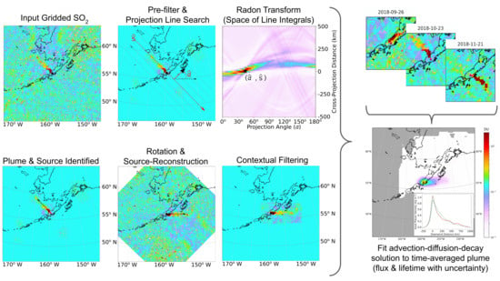
Mathematically this is accomplished by analyzing the Radon transform, used widely in medical tomography, signal processing of seismic data, and computer vision e.g., [19,20,21,22]. In this formulation, although it is vertical column density (VCD) that will be used to construct the time-averaged plume, we use the CrIS z-scores (Figure 1a) to define the necessary grid transformations owing to the beneficial statistical properties of the z-score compared with the CrIS-based VCD retrieval for weak plumes [6,16,23]. If UV-based data were used, the VCD estimate itself could be used instead.
For a gridded snapshot of z-score (), we define the Radon transform on the set of all lines in the plane as
where each projection line has been parameterized as
with t, an arc-length parameter, measuring true distance along the line. Here, s is the perpendicular distance from the origin to the projection line and the angle is the angle from the positive x-axis to the projection line normal vector which is also the angle between the positive x-axis and the line segment of length s perpendicular to (Figure 1c). The tangent vector of is . From the transformed map or “sinogram" (Figure 1d), we define the special point
which corresponds to the line that most reflects an elongated plume in the image with the projection vector . We then construct a profile of the mapped z-scores along this line:
Because this profile is taken along a straight line, it does not accurately capture the plume axial profile since the plume axis may be curved or distorted by the flow as in the subtle von Kármán vortex street distorting the plume axis in Figure 1 and Figure 2. To account for this, we search the space of nearby profile lines that are parallel to and extract the maximum value of the z-score for each value of t across all of these lines. This gives an approximation to the plume axial profile, though it is slightly foreshortened locally where the real plume axis makes excursions from the line . Once the overall profile is constructed, negative values are removed and the profile is normalized (Figure 2a). We then compute the 10th, 50th, and 90th percentiles of this modified profile, respectively. Based on the asymmetry of the 10th and 90th percentiles about the median, we accept or reverse the projection direction to determine the plume dispersal direction, reflecting the assumption that the plume is most concentrated near the source and is more dispersed in the downwind direction, that is, the profile is skewed downwind (Figure 2b).
With the projection direction now matched to the plume dispersal direction, the plume source must be estimated. As mentioned above, the approximate source region is meant to describe the location of the source region relative to the plume’s current configuration, meaning it may have been advected some distance away from the volcano after emission by the time of imaging. To estimate this position along the profile, , we exploit the simple one-dimensional advection-diffusion-reaction model (detailed below) which we use to estimate based on an estimate of the Peclet number and upstream-downstream mass partitioning for the profile (Figure 2c,d). This technique is detailed in Appendix A.
From these estimates, the source position is taken as in the projection coordinates and the Cartesian coordinates of the source position can be found from Equation (4a,b). The Cartesian grid coordinates are then translated so that the source is at the origin and rotated so that the dispersal direction is in the pre-specified direction (Figure 2e,f).
2.1.2. Filtering and Smoothing in Wind Reconstruction
Within this plume rotation and source reconstruction technique, several additional steps are taken to improve the quality of the reconstruction. At multiple stages detailed below, we make use of exponential smoothing kernels (Appendix B) rather than Gaussian smoothing or other types of smoothing for two reasons: (i) exponential smoothing reduces noise variance to a greater extent than Gaussian smoothing [24], and (ii) the exponential dependence in our chosen physics-based model suggests that exponential smoothing will only minimally distort the edges of the plume data.
First an attempt is made to remove background which may come from a bias in the noise or from anthropogenic sources. Since the volcanic plume occupies such a small fraction of a given grid, we first subtract the grid mean value from all pixels. Next, we filter the grid with a special filter designed to heavily weight measurements that are close to the volcano and are also in a neighborhood of the strongest detections (Figure 1b). This two-part filter is constructed as follows.
First, a radial weighting filter is constructed from a truncated radial Gaussian function centered on the volcano in question:
This weighting filter has unit weight at the volcano and is zero outside of the radius . This multiplicative filter is designed specifically to heavily weight plumes within (the standard deviation of the Gaussian) from the volcano. This filters out that has drifted into the edges of the image from other sources as well as plumes from the target volcano that were emitted previously to limit the possibility of double counting. We use this radially decaying weighting filter instead of a fixed search radius because it allows for variations in the wind speed which may advect puffs of to variable distances away from the volcano.
The second filter component generates a buffer around all z-score values above a threshold value (). This is accomplished by generating a binary map of all z-scores above the threshold and then convolving the binary map with an exponential kernel (K) with 20-km e-folding radius. A binary image is then generated to indicate where the numerical convolution result is nonzero and then this new binary image is again convolved with the same exponential kernel. The resulting map is of unit weight over a buffer patch very close to the high-confidence detections and decays to zero over a distance of approximately 50–100 km. This buffering weight () can be summarized mathematically as
where is the indicator function for the specified region and the convolution is understood to be performed numerically with a compactly supported kernel K. In our modular framework, if UV-based data were used instead of the IR data used here, the VCD estimate itself along with a threshold value for significance would be used to construct this filter.
An overall weight () is constructed as the point-wise product of the detection buffer weight and the radial weighting filter (, Figure 1b). As a last step, we multiply this overall weighting map by the original z-scores and perform a minimal smoothing by convolution with another exponential kernel of only 4-km e-folding radius to generate a smoothed and filtered z-score image which can be more readily analyzed by the above method to find plume-like clouds near the volcano (Figure 1c).
This filtered and smoothed z-score image is only used to define the necessary grid transformations to reconstruct the plume as detailed above. Once this is complete, the raw z-score image is interpolated onto the new grid (Figure 2g). A final filtering and smoothing step is performed after rotation and re-gridding. This step involves the binary image segmentation (specifically, connected-component labeling) of the buffered detection region computed for the rotated and re-gridded z-scores. Although we use the Python-based SciPy multidimensional image processing package, similar algorithms are available in most modern code libraries. From this, we keep only the connected detection region which contains the re-gridded origin (plume source). All other pixels are set to zero and the result is smoothed with a 4-km e-folding radius exponential kernel (Figure 2g).
2.1.3. Time-Averaging and Post-Processing
After grid transformation as described above, we construct the estimated VCD for each plume snapshot and average together all available snapshots in the time-averaging window. As a final step, the time averaged grid is translated so that the maximum time-averaged VCD value is at the volcano. This process is meant to reconstruct an empirical model of the plume from the volcano under conditions of constant emission, wind field, mixing, oxidation, and dilution.
2.2. Physics-Based SO Cloud Fitting
Here we present a very simple physical model for the continuous point release, dispersion, and evolution of a cloud of subject to a constant wind field which we will use to throughout this work to estimate the volcanic flux. The proposed model and its solutions are well known in the literature and can be found in or synthesized from the elements of many texts on environmental fluid mechanics e.g., [25,26,27].
We model the continuous point release of and incorporate constant advection, Fickian turbulent diffusion, and first-order reaction kinetics representing total loss of from the cloud as an advection-diffusion-reaction Equation (ADRE):
where u is the (constant) wind speed, k is a first-order reaction-kinetic decay rate, is the downstream eddy diffusivity, and are the aspect ratios comparing the downstream eddy diffusivities to those in the crosswind horizontal and vertical directions and S is a source term describing continuous point release of from the origin with mass flow rate . In this section, z refers to a vertical coordinate and not z-scores used elsewhere in the text. Note that as in [28] the chemistry (decay) term represents the loss due to actual processes (oxidation and conversion to sulfates, dry and wet deposition) as well as apparent loss related to dilution of the cloud below the sensor detection threshold. In this very simplified model, we have assumed that all eddy (turbulent) diffusivities are Fickian, that is, they are constants for a given analysis, or alternatively, they change sufficiently slowly that differences are not relevant over the time period of analysis. Other than the diffusivity aspect ratios which directly control the cloud’s spread, the shape of the cloud is also governed by the Peclet number of the flow which is typically defined as the ratio of advective transport to diffusive transport. Since the problem is set in an unbounded domain ( dispersion from an elevated point source in free atmosphere), there is no single characteristic length. In this study we choose as a characteristic length, the “e-folding distance” ()—the distance traversed in one e-folding timescale () under constant advection. This length scale, the distance over which a puff of decays by a factor of e in constant wind, is the primary measurement that previous studies have used to estimate the lifetime given knowledge of wind speed e.g., [1,2,4,18]. We therefore define the Peclet number for the problem as
This Peclet number controls the plume’s elongation in the wind direction and the upstream-downstream distribution of mass.
2.2.1. Application of Simplified Theory to Satellite Measurements of Volcanic Plumes
Although the governing ADRE can be used to describe a wide variety of elementary flows, we focus on analysis of the cloud produced by a continuous point release of in a time-averaged sense. As long as the time-averaging interval is much larger than characteristic changes in the cloud between the time interval endpoints, the time-averaged ADRE is asymptotically equivalent to the steady state ADRE with a constant source flux. We focus on this steady state solution in the present work since we will be analyzing time-averaged plume data integrated over time intervals much longer that the timescales of meaningful cloud dynamics predicted by the transient model (Appendix C). Additionally, from the perspective of a satellite, the above three-dimensional model is not very helpful for a trace gas like for which there is little or no vertical profile information. Consequently, most space-based measurements are of VCD, denoted here as . This measurement destroys any dependence on the vertical diffusivity (and consequently the parameter ) since the VCD is a quantity integrated over the entire vertical coordinate space after [27]:
where the following shorthand has been used:
and is the zero-th order modified Bessel function of the second kind. Here v is the average velocity of transient perturbations (Appendix C) and describes the excess dissipation caused by reaction and turbulent diffusion processes and is an elliptical radius measuring contours of constant dispersion in the absence of wind. Of significant importance for model fitting, the parameters in this equation do not form an independent basis. In particular, there is not unique dependence on the downstream eddy diffusivity (). To clarify this point, we rewrite this solution in terms of independent parameters only:
where , , and with .
This VCD model, equivalent to the solution for an infinite column source at the origin, depends only on the parameters , , , and . If space is re-scaled by the characteristic length (i.e., ), it is easily demonstrated that shape of this cloud is governed only by the crosswind aspect ratio and the Peclet number since and .
2.2.2. Relationship to Previous Fitting Model
By contrast to the ADRE solution used here, the fitting function of [2] can be written as where the Gaussian plume solution () approximately solves the steady ADRE in the high Peclet limit in which stream-wise diffusion and decay are neglected:
As described earlier, this approach from [2] enables the fitting function to accommodate some mass upstream of the source and to spread out downstream although it is heuristic, lacking a direct solution from the physics of the ADRE. The 2D EMG model has the property that its peak is downwind of the source. This could be a useful property if the average lag time between emitted pulses and satellite overpass could be estimated. Since this is not known, our plume source-reconstruction approach is more flexible since it more closely approximates upstream turbulent mixing and is better suited to examining persistent point source emissions. Additionally, this fitting model has exactly the same issues related to fitting non-uniqueness as the ADRE used here, requiring independent estimation of one of the geophysical parameters, that is, the flux, wind speed, decay rate, and measures of spread are sought, but one of these must be estimated independently. In previous studies using wind data, the wind speed is estimated and the other parameters are fit.
2.2.3. Fitting the ADRE Parameters
Although the VCD model could itself be fit to time-averaged satellite VCD observations in a similar manner as in [2,4,5,12], the signal to noise ratio can be improved by another integration, specifically integrating through the crosswind (y) direction as in [1,11,12,18] to generate a line density. Although this will destroy information related to the crosswind aspect ratio , this has no effect on measuring the distribution of mass upstream and downstream which is of greater consequence than measuring the aspect ratio. Additionally, once the line density parameters are fit, the aspect ratio can be estimated by other means (Appendix D). Because the main parameters of interest to the present work are estimates of the flux , the lifetime , and to a lesser extent the Peclet number of the flow, integrating out the crosswind dependence will not significantly impact the estimation of these metrics. In practice, we integrate over the standard deviation width of the time-averaged plume which we determine by first integrating in the downwind direction and then treating as a probability distribution. Performing this integration gives the profile of mass per distance downwind contained in the plane perpendicular to the plume axial line or wind vector:
As VCD refers to the density of the species contained in a vertical column, we refer to this quantity (a line density of in planes perpendicular to the plume axis) as the axial planar density (APD).
The one-dimensional APD solution is equivalent to the solution to the three-dimensional governing equation for an infinite planar source at . This integration provides four significant benefits: (i) APD data have a stronger signal to noise ratio than VCD data yet preserves the same parametric dependence on , , and as , (ii) The use of APD instead of VCD eliminates the possibility of model error due to data asymmetries in the crosswind direction, (iii) Regardless of the crosswind eddy diffusivity aspect ratio, the upstream-downstream mass partitioning will not be affected so an accurate Peclet number can still be computed from APD fitting and (iv) the high signal-to-noise ratio and simpler functional form make nonlinear fitting of to APD data more likely to converge owing to the ease of generating high-fidelity initial parameter estimates compared with what is required for fitting to VCD data.
Because of these benefits, we construct an APD profile from the time-integrated plume VCD and then fit to it the model . With these fitting parameters, we can immediately calculate the plume Peclet number as . An important benefit of this model is that functionally, it is an exponential decay upstream and downstream with a matched point at the source. Exploiting this simplicity, we fit a log-transformed APD profile rather than the APD profile itself since this is closely related to linear regression up- and downstream with approximately Gaussian error, enabling the use of traditional fitting metrics such as the coefficient of determination () without incurring the significant difficulties in interpreting nonlinear regressions this way e.g., [29].
To estimate the degassing flux (), we must independently estimate one of u, k, , or . If, as in similar studies e.g., [1,2,3,4,5,11,12,18], wind data is already used to construct the time-averaged plume, then the mean wind speed could be used compute from . Here, we focus on the decay rate k since to first order, it can be estimated directly (with uncertainty) from the record of individual plume snapshots that make up the time-averaged composite. Once this is estimated, the quantities of interest () are determined from the parameter estimates () by
where the quantities of interest are and .
2.2.4. Decay Rate Estimation
From [6], the CrIS total mass (M) is a normal random variable as is the time derivative . Consequently, if we restrict analysis to periods with , the decay rate (k) and the lifetime () are both ratios of normal random variables with an almost certainly non-zero variable as the denominator. Ratio distributions of this type can be approximated as being lognormally distributed [30]. The distributions of estimated lifetimes from major sources globally in [3] exhibits an approximately lognormal shape, lending evidence for the implementation of a lognormal model. We use this fact to compute a lognormal PDF for likely values of the decay rate for each time-averaged plume and propagate that uncertainty to construct a similar PDF for the mass flux and other variables as well.
Since a lognormal distribution is parameterized by the Gaussian parameters of the log-transformed variable, we estimate the parameters of the lognormal distribution using the valid log-transformed decay rate samples. We generate our decay rate samples from the time series of plume observations in the time-integration interval using the simplifying assumption that whenever the cloud mass in the domain is decreasing, the flux of from the volcano at that time is much less than the magnitude of the mass loss rate. Such an assumption is related to treating the time-averaged plume as the average of a series of discrete puffs. This is a reasonable assumption for lower-middle tropospheric injection where the lifetime is generally regarded as being significantly shorter than for major eruptions injecting into the upper troposphere or stratosphere. Since smaller, less-powerful emission is the target activity, the conditions of this assumption appear reasonable.
This approach yields samples of the decay rate as
for all i where and is the i-th total cloud mass in the sequence of plume images. Note that in this scheme, the maximum value of the samples is limited by the time interval as which always occurs when the cloud mass decays to zero (i.e., , or apparent 100% loss in one time interval). We then correct the samples by a specialized procedure detailed in Appendix E which accounts for this hard upper limit (right-censoring). The corrected samples are then used to estimate the parameters of the lognormal distribution for the decay rate.
2.3. Uncertainty Quantification
From [6], CrIS VCD data generally agrees very well with high-resolution data from TROPOMI for small to moderate columns (<50 DU) and tends to underestimate very large TROPOMI columns by about 25% consistently across a variety of scales. Because the vast majority of the data analyzed here are below this threshold and TROPOMI data uncertainties are approximately 30–50% of those of OMI [13], we estimate that the errors originating from the use of CrIS to compute total cloud mass are somewhat less than those from OMI. We estimate the uncertainty on the CrIS VCDs in each plume image as approximately 14% for these relatively dilute plumes and as much as 20% for plumes with a large fraction of columns DU, though these are uncommon outside of significant eruptive events. The estimation of VCD from z-scores is expected to have a very small impact on total error.
In the absence of errors due to the rotation, the uncertainty from stacking multiple images should decay as the number of stacked images increases, specifically decaying as . Ref. [3] estimated errors from the NWP wind rotation technique as approximately 6% for wind speed and direction and approximately 20% for wind height. Similar to [3], varying the detected wind direction with uncertainty of yields approximately 4–7% variation in our time-integrated plume. Additionally, our source reconstruction technique yields between 17–35% variation compared with the traditional approach without source reconstruction-based wind rotation.
Additional error is incurred due to the highly unsteady nature of volcanic emissions. Compared with anthropogenic sources, volcanic outgassing is highly variable, varying by orders of magnitude on a variety of timescales e.g., [31,32,33,34,35,36]. In our simple dispersion model, the fitting solution is the result of time integration of a dense sequence of discrete puffs, which is at least somewhat accurate to nature; however, error is incurred whenever the time delay between a new discrete puff and the next satellite overpass is maximized, that is when a discrete puff occurs just after an overpass. This error is due mainly to the chemistry and turbulent diffusion effects which both dissipate the concentration and total mass of the puff by some amount when the next overpass occurs. Because at low altitudes the lifetimes are on the order of hours, significantly less could possibly be measured in the next overpass for that puff than if the puff happened just before an overpass. In general, for a re-imaging time of T and an lifetime , the fraction () of puff mass that can be observed at imaging time for a puff emitted at in the re-imaging interval is . Assuming that puffs are uniformly distributed in each imaging window, the expected value loss for a given puff is by the time it is imaged for the first time. For an lifetime of 6 h e.g., [3,13] and a re-imaging window of 12 h, each puff will have decayed by an average of approximately 57%. Fortunately, this theoretical error propagates only minimally to the decay rate estimation since that is already based on relative loss, so such a consistent bias factor will play little role. If there were just a single puff released in an interval this error would be inherited in the accumulation of the time-averaged plume; however, the more puffs released, the more total mass is accumulated. In the limit of an infinite number of puffs in a re-imaging interval, the steady state fitting function would be an accurate representation of the measured distribution of and this error would be zero theoretically. Although we do not derive a theoretical correction factor to describe this effect, based on the formula above, we estimate that this loss factor is approximately % where the variation is derived from considering h. This yields a uncertainty contribution from this factor of approximately 32%.
Combining these sources, we estimate that the total uncertainty on the time-averaged plume is between 37–48% over a wide range of averaging periods and only 18–36% if the effect of emission-measurement asynchrony is determined to be negligible. As described above, we fit an APD model rather than a VCD model which greatly improves the signal to noise ratio of the data. Fitting uncertainty is reduced with respect to VCD fitting and as with the time-averaging procedure, decays as inverse of the square root of the number of crosswind measurements, yielding a fitting uncertainty which is much less than these other sources.
Uncertainty in the decay rate estimation is derived mainly from uncertainty in the CrIS VCD data which is amplified somewhat by a fairly noisy decay rate estimation process (Appendix E). Even if all CrIS VCD data have the larger uncertainty of 20% and the total mass integration domain only includes about 900 measurements ( pixels), the maximum uncertainty on the corrected decay rate samples is only about 10%. All remaining uncertainty on the decay rate is accounted for by representing the decay rate as a lognormal distribution. Owing to the maximum base uncertainty on the samples, we impose a minimum 10% uncertainty on the decay rate lognormal distribution.
Lastly, because the method used to estimate the decay rate is noisy, the uncertainty propagated to the quantities of interest from the decay rate (representation as a lognormal distribution with 10% minimum uncertainty) is much larger than the uncertainty from the fitting procedure and in most cases, the uncertainty from all other sources, though it is typically less than about 45% overall. Although this assumes that all errors discussed here are uncorrelated, which may be violated in some cases, the probability dispersion present in the decay rate distribution alone still likely accounts for most of the total uncertainty. For comparison, uncertainty on previous state-of-the-art annual emissions have been estimated as 55% for stronger sources (>100 kt/yr) and 67% for weaker sources (<50 kt/yr) e.g., [3,5].
Because each parameter of interest is proportional to k (Equation (16)), the retrieved PDFs of these parameters will inherit the decay rate’s lognormal distribution. Specifically, the decay rate is distributed as
where the lognormal distribution is parameterized by and , respectively, the mean and standard deviation of . As described above, we impose a minimum uncertainty (here, coefficient of variation) for the decay rate, constraining the value of as , derived from the parameterization of the coefficient of variation for a lognormal variable. Each parameter of interest is therefore distributed as
and the lifetime is distributed as
3. Results
As described above, one of the significant benefits of developing these techniques for IR sensors is the ability to fill gaps in the UV-based record at high-latitude volcanoes in the winter when there is insufficient UV backscatter to make reliable measurements. Additionally, at high-latitude volcanoes, CrIS swaths from each JPSS satellite overlap significantly, providing at least 4 complete scans over a target volcano per day from NOAA-20 and SNPP combined. This high combined return rate and orbital coverage is ideal for increasing the signal-to-noise ratio of the time-averaged results. Below, we demonstrate these techniques for a 4-month period of unrest at Veniaminof Volcano between September–December 2018 (Figure 3).
3.1. 4-Month Summary of Eruptive Sequence
Between September and December 2018, Veniaminof volcano in the Aleutian islands underwent a period of unrest characterized by a sequence of small-moderate explosive episodes, lava flows, and a mix of passive and active emissions (Taryn Lopez pers. comm); [37]. Between September 3–4 the Alaska Volcano Observatory (AVO) raised its aviation color code (ACC) and volcano alert level (VAL) from Green/Normal to YELLOW/Advisory and then to Orange/Watch based on an increase in seismic activity and reports and webcam footage of low-level pulsatory ash emissions. On 21 November 2018, significant explosive activity sent an ash plume to a height of 15,000 ft (4.6 km), sending ash 150 km downwind which prompted AVO to raise the ACC/VAL to RED/Warning. Other than this event, AVO maintained the Orange/Watch color code and alert level through the beginning of January 2019 when the activity stopped [37]. Throughout this period, height estimates retrieved from the probabilistic CrIS algorithm were dominantly below 4 km with several plumes exceeding 5–6 km over small areas (Figure 4b). This is an ideal eruption on which to demonstrate this new flux algorithm using CrIS data since the high SZA at this latitude significantly degrades the signal-to-noise ratio of UV-based data, preventing reliable analyses of this type. Using IR data, like that from CrIS, is the only way to measure the flux consistently throughout this interval particularly between the early and late stages of this eruptive sequence.
As described above, this algorithm uses a radial Gaussian search weight parameterized by a soft search radius () with a hard cutoff at rather than a single hard search radius cutoff as in [3,13] and others. For the case study of Veniaminof, we used a soft search radius of 150 km, meaning that there is a hard cutoff at 600 km and that theoretically 95% of the dispersing plumes should be located within 300 km. Although this search is used to determine the wind-reconstruction, the stacked data spans over a box 1000 km × 1000 km. Over this 4-month eruptive period, SNPP and NOAA-20 together collected 493 plume snapshots comprising about VCD estimates, generating the time-averaged plume in Figure 3 with fitting results summarized in Table 1. Although the VCD values used here are estimated from the gridded CrIS z-scores (Figure 4a) and a conversion factor generated only from the most robust retrievals, there are enough samples to make a credible time-average. Despite this, there is still a subtle bend in the plume axis, which is the result of accumulating many plumes which themselves have been dispersed in complex wind fields (e.g., the individual plumes in Figure 4a). This crosswind asymmetry justifies the theoretical benefits of performing the fitting on an APD profile (Figure 3 inset) rather than a VCD grid.
3.2. Time Series of 10-Day Running Averages
Although this capability is useful for long-term flux estimation, using a shorter time-averaging window could make this estimation relevant to operational users such as volcano observatories. However, a shorter time-averaging window necessarily induces a lower signal-to-noise ratio. Because of the large volume of data used to make each average, even much shorter time-averages contain enough data to make usable estimates. Here we demonstrate the construction of a time series of 10-day averages for the same eruption from Veniaminof (Figure 4). The benefits of fitting an APD rather than VCD model are even more apparent in this context since each 10-day average VCD at a given location only contains about 40 CrIS VCD estimates, compared with the approximately 1500 CrIS estimates within 300 km of the plume axis.
During this eruptive period, there were principally four episodes of heightened emission. In some cases, these were characterized by a single short-duration, but sustained emission (late September), whereas other periods such as the increased flux in mid–late November were characterized by a sequence of pulses. In some cases, the peak fluxes do not coincide exactly with known periods explosions and ash emission, most notably, the significant explosive activity during 21–22 Nov. during which the AVO ACC/VAL were RED/Warning yet the flux peaked 3 days later. This example is most likely an artifact of the centered time-averaging (±5 days), which captured not only this significant release which itself lasted approximately 2 days, but also the fact that there were greater emissions following this event than preceding it. The largest emission occurred in mid-December with significant plumes dispersing north and northeast. This period of emission is discussed in greater detail below. Overall, the 4-month averaged flux (blue dashed line, Figure 4c) is substantially similar to the average of the time series of fluxes (blue dotted line, Figure 4c), although they are not exactly comparable owing to the statistics of lognormal variables. Although this capability yields intriguing details of emissions during this poorly understood eruption, a full analysis and geological interpretation of this eruptive sequence are beyond the scope of this work.
As described in Section 2.2.4, the decay rate and lifetime are approximately lognormal variables as predicted by theory and as evidenced by the distribution of lifetime estimates from a global catalogue of large sources [3]. At several points in the time series, particularly until mid-October, there are not enough substantial plumes in the time-averaging interval to make a credible estimate of the decay rate and lifetime (Figure 4e). For such intervals in the middle of the time series, the previous interval’s statistics (omitting flux) are used as defaults. For the earliest interval, we have used the global distribution of lifetimes from [3] to estimate the default lognormal parameters. As is evident later in the time series, the range of estimates for lifetime are very similar to the statistics of the lifetimes fitted by [3].
4. Discussion
4.1. Estimated Cloud Mass
Although geophysical parameters such as the flux, lifetime, and diffusivities are presented here as lognormal variables with uncertainty propagated directly from the decay rate estimation, the plume mass and Peclet number are direct result of the fitting and have uncertainty dominated by the fitting error. Owing to the statistics of lognormal variables, the median fitted plume mass can be calculated as the product of the median flux and median lifetime. Figure 4e shows the 10-day average cloud mass (blue) that would be estimated using only the detection steps introduced above, but not the stacking, that is, it is the 10-day average of the individual plume detections. This is a very conservative estimate since it does not include any below the z-score-based robust detection limit. For the plumes in this time series, this is about 40% of the fitted cloud mass (Figure 5).
Crucially, if the individually detected cloud masses could accurately incorporate regions of low-concentration surrounding the robust detections, then a plausible flux estimate could be made from a sequence of measurements simply by estimating the decay rate as in this work. However, clearly a significant amount of the total in these small clouds is too dilute for the robust detection and the rotation and stacking is required to amplify the signal in these regions.
4.2. Wind Speed, Goodness of Fit, and Anomalous Flux
For the 4 month-averaged plume, the fitted wind speed agrees very well with radiosonde wind data from Cold Bay, Alaska, located only 235 km to the southwest (Figure 6, data provided by Larry Oolman at the University of Wyoming Weather Lab, http://weather.uwyo.edu/upperair/sounding.html (accessed on 30 December 2020). Here we have analyzed all available soundings for the 4 month period, using only the data between 2 and 5 km altitude, which is the typical range of altitudes measured by CrIS during this period. The 4 month-averaged radiosonde wind speed was 13.0 m s and the median (and 90% confidence interval) radiosonde wind was 11.8 (3.6, 26.8) m s which compares very well with that from out fitted plume of 12.0 (6.1, 23.4) m s. At this large temporal scale, agreement is very good; however, this technique is not a robust tracer of time-averaged winds at finer scales.
As demonstrated by comparing Figure 4 and Figure 6b, the fitted wind speeds over 10-day intervals are generally significantly less than those from radiosonde winds. Principally, this discrepancy is the result of the fitting process based on plume shape, requiring a substantial enough plume to be present. Furthermore, the fitting is not a direct measure of the wind speed since any upwind dispersal (real or apparent and caused by smoothing) will greatly reduce the fitted wind speed. If more plume observations are incorporated, the time-averaged dispersal behavior emerges, yielding a much more accurate fitted wind speed. Fortunately, this discrepancy has little impact on the fitted flux and lifetime since lifetime is estimated independently and the flux is proportional to the fitted cloud mass, itself very accurate when the fit is good. When the fit is degraded, the fitted cloud mass (and thus flux) can be affected by the fitted wind speed.
Over the sequence of plumes from Veniaminof described here, the APD model fit is generally good with an or better (Figure 4c). Critically, there is no apparent correlation between and flux; however, there is an apparent negative correlation between the wind speed estimate and for the most wind-affected plumes (Figure 4d). This typically results when the APD profile does not decrease smoothly in the downwind direction despite a very good fit (qualitatively) in the upwind direction. Owing to the simplified physics used, it could be possible to make a more robust estimate of the Peclet number and flux using only the physics of upwind dispersal; however, such a specialized fit is beyond the scope of this work.
As described, the largest emission occurred in mid-December, reaching peak emission rates of 8.6 kt day. Through this period, the fit worsened somewhat to . Although many significant plumes can be seen in individual CrIS overpasses during this time (Figure 4a), it is possible that the fluxes during this period are overestimated as a result of an overestimated wind speed. If the wind has carried at an irregular speed or if the interval is characterized by a few large, discrete releases, it is very common to observe highly irregular (non-smooth) decay in the downwind direction. As the APD model attempts to fit the far-downwind that has not dispersed or diluted, the resulting fit is an apparently more wind-affected plume containing greater total mass and thus greater apparent flux with a poorer fit (Figure 7). Regardless of these considerations, the fitted model is still plausible throughout this period suggesting that the true fluxes were likely similar to those fitted here.
4.3. Comparison of Single-Sensor Results
Throughout, we have combined retrievals from NOAA-20 CrIS and SNPP CrIS. Here we demonstrate that these two sensors make consistent measurements by generating a 4-month averaged plume and fit for each sensor separately (Figure 8). The time-averaged VCD maps are largely similar with the NOAA-20 CrIS version extending over a slightly larger area downstream and the SNPP CrIS plume narrowing downstream and containing smaller peak VCD values than the NOAA-20 version. The fitted parameter values (Table 2) reflect these observations. The eddy diffusivities estimate for the combined analysis was significantly larger than for the individual sensors, in particular in the crosswind direction. This is due to the fact that combining the two sensors worth of observations can only increase the spread of the time-averaged VCD, mimicking the effect of mixing by large eddies. All other parameters were constrained between the NOAA-20 and SNPP fits; however, the combined fitted parameters are more similar to those of NOAA-20 than SNPP despite the fact that there were roughly the same number of NOAA-20 and SNPP observations.
4.4. Comparison with Other Estimates of Degassing and Lifetime
Although there are not any direct comparisons possible for this case study due to the limited coverage by UV instruments which typically make these measurments, we note here two promising comparisons that are available. In analyzing flux estimates from TROPOMI data, [13] compared annual emissions from a variety of large sources in the interval April 2018 to March 2019, including Veniaminof. They measured the annually averaged flux from Veniaminof in this period as kt yr (TROPOMI), kt yr (OMI), and kt yr (OMPS) which are in decreasing order of resolution and average sensitivity per area. Based on the 4-month CrIS-based estimate of kt day, CrIS measured a total of 183 kt over the course of the 2018 eruption. If very little or no emissions occurred in the other 8 months of the year, this would compare well with the estimate from TROPOMI in [13]. However, over the previous decade (2008–2017), annual average emissions from Veniaminof were approximately kt yr as measured by OMI for NASA’s public archive https://so2.gsfc.nasa.gov/measures.html (accessed on 29 December 2020) [38]. If this low level of emissions had occurred through the rest of the year, the annualized emissions from Veniaminof would be approximately kt yr. Depending on which of the above UV measurements is most similar in sensitivity to CrIS, this annualized flux is between 19% and 236% greater that what was recorded with UV instruments although this comparison is probably most appropriate for CrIS-OMI (209%) and CrIS-OMPS (236%). Because about 100 kt of the was emitted in December when SZA was too high to make reliable UV measurements for all but the strongest plumes, it should be expected that CrIS would measure about double the annual flux as OMI and OMPS including a period of unrest occurring in the winter.
Lastly, as described throughout, the lifetime or decay time scale plays a central role in determining the flux. Consequently, our estimation technique for the decay rate outlined in Appendix E must be compared to other estimates. The most comprehensive data on plume parameters is compiled in the global catalog of large sources which includes a mix of volcanoes, coal-fired power plants, and smelting facilities [3]. The values of decay time scale in this catalog are the result of a similar wind-rotating and time-averaged fitting process, except that in [3], the wind speed is estimated independently of the fit using ancillary wind datasets and the decay time is fitted from the mean plume. Here, we adopt a completely different approach, estimating the lifetime from the record of individual plume mass observations, producing a lognormal probability distribution for the lifetime representing the uncertainty propagated from the noisy decay rate estimation process. Our distribution of lifetimes is in very good agreement with the distribution from the global catalog which contains data from 215 large sources (Figure 9). In particular, our distribution strays no more that 1% outside the 90% confidence interval for the distribution of the global catalog. We have generated this estimate using 10,000 empirical distribution functions (EDF) of simulated lifetime sample sets (each with 215 members) drawn from the global catalog histogram.
The strength of this decay time scale technique is that it can be estimated solely from a sequence of plume observations; however, the uncertainty in the technique is significant and propagates to the other fitted quantities unless additional data is used to constrain the problem. Overall, the good agreement between the distributions of lifetime estimates from Veniaminof and those from large sources globally is an indication that this technique can produce similar lifetimes as are measured by other means and thus that our flux estimates are at least as accurate as in similar techniques.
5. Conclusions
- (i)
- Time-averaged volcanic flux and lifetime estimation techniques can be successfully modified to accept newly-available hyperspectral IR data, enabling robust gas monitoring at high-latitude volcanoes in all illumination conditions, including low- or no sunlight conditions. This has the potential to fill a key observational gap in traditionally UV-based monitoring.
- (ii)
- Our technique detects weak signals of plumes in gridded data using computer vision and object-detection techniques used widely in medical and seismic tomography. It then amplifies these weak plume signals by attempting to reconstruct the wind fields dispersing them and time-averaging the results. This amplification enables the recovery of approximately twice as much mass as would be estimated by considering the cloud mass in individual plume snapshots alone. A new line-density fitting function derived directly from the time-averaged point-source dispersion physics is used to generate a well-fitting model of the time-averaged plumes.
- (iii)
- The decay rate and lifetime (reciprocal decay rate) are estimated independently of the fitting and are shown to have lognormal statistics which agree remarkably well with previous published estimates of the distribution of lifetimes from large sources globally.
- (iv)
- This technique can be subdivided, allowing for short-timescale averages and the generation of flux monitoring time series, which could prove useful to observatories. The technique in general and the time series capability in particular have been demonstrated for the September–December 2018 period of unrest and eruption at Veniaminof volcano, Alaska, highlighting the importance of new algorithms designed for detection and characterization of in the infrared.
Author Contributions
Conceptualization, D.M.R.H. and M.J.P.; methodology, D.M.R.H.; software, All authors; validation, D.M.R.H.; formal analysis, D.M.R.H.; investigation, D.M.R.H.; resources, All authors; data curation, J.S.; writing—original draft preparation, D.M.R.H.; writing—review and editing, All authors; visualization, D.M.R.H.; supervision, M.J.P.; project administration, M.J.P.; funding acquisition, M.J.P. All authors have read and agreed to the published version of the manuscript.
Funding
This research was funded by the JPSS Proving Ground and Risk Reduction (PGRR) Program of the National Oceanographic and Atmospheric Administration, grant number NA15NES4320001.
Institutional Review Board Statement
Not applicable.
Informed Consent Statement
Not applicable.
Data Availability Statement
The Level-1B CrIS spectra used in this study for retrieving properties are available from Goddard Earth Sciences Data and Information Services Center. GES-DISC, https://disc.gsfc.nasa.gov, (accessed on 22 December 2020); [39,40]. The property retrieval algorithm can be found in [6].
Acknowledgments
The authors wish to thank Taryn Lopez for sharing insights on the remote sensing view of the Veniaminof eruption from a variety of sensors as well as all members of the JPSS PGRR Volcanic Hazards Initiative team for feedback on product development. We additionally thank Larry Oolman for the availability of radiosonde data. We thank the two anonymous reviewers for their helpful comments on the manuscript. Disclaimer: The views, opinions, and findings contained in this report are those of the authors and should not be construed as an official National Oceanic and Atmospheric Administration or U.S.Government position, policy, or decision.
Conflicts of Interest
The authors declare no conflict of interest.
Appendix A. Plume Source Estimation for Rotation and Source-Reconstruction Scheme
As in the main text Section 2.1.1, once the plume dispersal direction is found using the best fitting projection line () derived from the Radon transform of the input z-score image, a profile of the z-scores () along this line is constructed from nearby parallel profiles which approximates the plume’s axial z-score profile. Here, t refers to distance along the profile line. We then censor negative z-scores as noise and normalize the profile:
which has the properties of a probability density function (Figure 2a). As in the main text, from we compute , , and , the 10th, 50th, and 90th percentiles, respectively. If , then the imaged plume is extended downwind in the direction of . If the opposite is true, then the plume is dispersed towards so the projection direction and z-score profile are reversed (Figure 2b).
As described in the text, estimation of the plume’s source location requires an estimate of the Peclet number for the single plume observation generated from this profile . Although the APD model () is not an axial slice of a VCD cloud, we compare it to the computed profile () and make a rough estimate of the Peclet number as:
where is an estimate of the mean gradient of the natural logarithm of the profile to the right of the profile maximum and is an estimate of the mean gradient of the natural logarithm of the profile to the left of the profile maximum (Figure 2c).
To see this, consider that from the APD theory,
and consequently,
Solving for yields this formula for the Peclet number in terms of the left and right-side gradients.
In the context of the normalized plume axial profile , the peak of the profile is not necessarily located at the profile line origin and so we use left and right partitions about the location of the maximum (). Additionally, because each plume observation is noisy, we do not compute and directly as the derivatives and , respectively. Instead, we use the slopes of independent linear fits to the right and left sides of to estimate and . We restrict the data used for the fits to the nearest continuous non-zero intervals on either side of . In concert with the other techniques detailed in the text, this ensures that only data from the continuous plume is used for the fit and does not incorporate any from unrelated sources or from previous emissions that may have been caught incidentally in the profile.
We now explain the rationale behind using the one-dimensional representation (APD, ), rather than an axial slice of the two-dimensional VCD solution (). We note here that the VCD solution can only approximate the cloud VCD away from the source since there is a singularity there and this is clearly unphysical. Additionally, the measurement FOV or pixel represents a fundamental limitation on resolving the trend toward a possible singularity even if one could exist. Consequently we may look to estimate the Peclet number by using the data away from the source region.
Using a common first-order approximation to (modified Bessel function of the second kind of order zero) from the formula for the VCD solution in the text, the VCD cloud can be approximated away from the origin with elementary functions:
Away from the source region, the quantity changes very little in the x-direction compared to the exponential quantity in the approximation. Furthermore, the x-derivative of the logarithm of this quantity is negligible compared with that for the exponential quantity. As a result, the quantity for an axial profile of the VCD is well-approximated away from the source using the profile of APD instead which includes only an exponential term and is therefore well-suited to linear regression in a log-transformed space.
There are two alternative (but flawed) methods that we could employ to attempt to rectify this inconsistency. The first method would entail multiplying the term onto before taking the logarithm when constructing the right and left side gradients (). This would theoretically eliminate the singularity present in the axial profile of the approximate VCD solution above (). However, as described above, there cannot be any singularities in the VCD data, so this approach would introduce a singularity in the source reconstruction analysis at . The influence of this singularity on nearby data would make fitting of these gradients very unlikely to be accurate even if the fitting process did converge. We could do the fitting away from , but this would exclude the most reliable data since larger values in the CrIS retrieval have a lower coefficient of variation.
A second method would be to directly fit an APD profile to the data before source reconstruction once the plume dispersal direction is found. We do not use this approach for two reasons: (i) using just a single axial slice of the cloud allows us to filter out nearby puffs of from other sources and prevents double-counting of previous puffs from the studied volcano which may be lingering within the image and (ii) because there is sufficient noise in a single plume image to significantly disrupt the construction of a smooth APD profile. If this were possible, the time-averaging process would not be necessary and the temporal resolution of the degassing flux calculations would simply be the repeat time of the sensor. Even cursory investigation of plume images demonstrated that the level of noise for a single plume image is too great for this method to be employed.
Once a rough estimate of the Peclet number is generated, we compute the source location using upstream-downstream mass partitioning. The APD model predicts the fraction p of the plume mass that will be found upwind of the source location as
The source location is then found from
as in Figure 2d. This can be computed by inverting the cumulative distribution of to find the th percentile (pth quantile) value of t along the profile. This procedure is preferable to setting the source location as the location of the maximum point since the maximum can be significantly dislocated with respect to the spatial decay of the plume strength owing to a variety of factors including complex distortion by local winds and simply retrieval error and noise.
Appendix B. Exponential Smoothing Filter
As demonstrated by [24], the use of an exponential kernel for smoothing reduces noise variance to a greater extent than a Gaussian kernel. The exponential kernel used in this study corresponds to the exponent-1 member of the family of exponential filters from [24]:
where is the e-folding radius, that is the radius at which the kernel has decreased by a factor of e. In the context of and exponential probability distribution, is also the mean and standard deviation radius.
For practicality in pixel smoothing, the kernel is implemented as a square array where N is determined as follows. For a specified , a tolerance is set which corresponds to the fraction of kernel mass outside a maximum radius R which can be computed from:
Inverting this to solve for R in terms of requires use of the non-principal branch of the product-log or Lambert W function ; [41]:
Because we are interested in small values of , we use the following three term approximation for the specified branch of as in [41]:
for some real variable , yielding the following approximation for R:
From this value of R, we compute the discrete kernel width in pixels as the nearest odd integer (≥3) to the value of , where is the smaller of the x- and y- grid spacings. We then compute as above on the kernel domain: . Lastly, the kernel array is normalized so that it has unit sum.
Although this process leads to fairly large kernels (in number of pixels), the kernels are still highly concentrated. For example, using gridded CrIS data with 16 km pixels, specifying an e-folding radius of 20 km, and choosing a tolerance of yields a kernel which is 17 pixels wide; however, of the kernel mass is within 60 km of the center. At the edges, the kernel is only approximately -th of its value at the center and in the corners, the kernel is only 1/10,000-th of its value at the center. The 4 km e-folding radius kernel (with ) used to smooth the rotated plume data is only of size .
Appendix C. Appropriateness of Implementing a Steady State Solution
The time required for the solution of a transient diffusion process to approach a steady state solution is referred to as the Local Accumulation Time LAT; [42,43,44] or Mean Action Time MAT; [44,45]. This timescale represents the time required for a bounded system to transition from one steady state to another due to a change in boundary conditions or for a disturbance to propagate past a point in an unbounded system tending locally towards steady state.
Here we estimate the MAT for the advection-diffusion-reaction problem used in the present work and demonstrate that the image repeat times and time-averaging intervals are sufficient to resolve the state of the plume over multiple imaging overpasses. Equivalently, we demonstrate that the MAT is typically less than the plume image repeat time for most small plumes and consequently each integration period (accumulating many plume images) can be treated as representing a steady state cloud.
From the text, the governing advection-diffusion-reaction equation is:
where the source () is a continuous point source of and the initial condition is uniformly zero. In this section, z refers to a vertical coordinate and not z-scores used elsewhere. Similar to the text with slightly different notation, the steady state (infinite-time) solution is
with the shorthand
To compute the MAT, we need the full, transient solution which transitions from the uniformly zero initial condition to the steady state solution:
As described by [44], the MAT is the local expected value waiting time for the distribution of temporal perturbations in the field, which is a good proxy for the waiting time to steady state, even though formally, diffusive problems require infinite time to reach steady state. In problems involving shock-like solutions, the MAT is equivalent to this waiting time. following [44], we define the MAT as
where the second equality is derived by integrating the numerator by parts, and using the zero-concentration initial condition. Because the steady state and transient solutions are known, we can compute the MAT directly:
The first integral can be found by substitution and then integration by parts:
where the substitution in the first equality comes from setting , and inverting to obtain .
The second integral is calculable from [46] (Equation 4.3.34):
Combining these results yields the MAT:
Because the shorthand parameter represents the distance from the source to a point on the ellipsoid scaled by the diffusion aspect ratios, or rather the true downwind distance for all points in the plume axial line, the mean velocity of source disturbances in the plane of the cloud is
The consequence of this is that for the considered flow, the mean propagation velocity of changes in the flux from the volcano source is greater than the mean wind speed by a factor greater than unity and that the wind speed may be used to construct an upper bound on the MAT for the disturbance to affect a given point.
For a fairly typical mean wind speed of 10 m s, the disturbance caused by a sudden change in the degassing flux will arrive at a point 500 km downwind (fairly far for typical degassing plumes) within at most h. This is exact in the limit as ; however for more typical plume Peclet numbers (), the MAT is between 2.2–11.7 h. As described in the text, a single CrIS sensor aboard S-NPP or NOAA-20, cannot reliably fully cover a plume’s extent in one overpass, typically requiring instead two or more precessing orbits to construct an image covering the plume’s full extent. For these satellites, the mean motion is ≈14.2 orbits per day, giving an orbital period of ≈101.4 min. For a plume image requiring two orbits, the imaging period is ≈3.4 h and the image repeat time is the time required for 7 orbits (≈11.8 h). Since the image repeat time is fairly close to the maximum possible MAT for the considered case and is longer than a typical MAT, the time-integration intervals encompassing several observations are certainly far longer than the steady state waiting time and consequently the steady state solution to the problem is an appropriate model from which to invert the source and cloud parameters.
Appendix D. Aspect Ratio Estimation
Once the one-dimensional fitting is complete, the diffusivity aspect ratio () can be estimated using the resulting fit parameters, specifically the fit value of . Specifically, We can construct two new profiles of the VCD data in the absence of wind. We define:
and
These two profiles can be computed from the VCD data using the fit value. Next we normalize these profiles so that they are non-negative and integrate to one:
and
In theory the aspect ratio can be computed from these normalized densities (both Laplace distributions theoretically) as the ratio of their variances:
Although we could have attempted to fit the VCD solution including the aspect ratio to the VCD data to obtain an estimate of the aspect ratio, this method is more robust since it allows that the mean wind may not have been perfectly straight or uniform, resulting in a mean VCD cloud that has an asymmetric crosswind mass distribution or is symmetric but displaced from the theoretical wind axis. This would result if there were non-uniform or non-straight-line winds dispersing the puffs near the volcano which is very common.
Appendix E. Estimation of Decay Rate Statistics
Decay Rate Correction
To estimate the decay rate (k), we consider the problem in the context of first order reaction (loss) kinetics, that is, as a reactor model for the total cloud mass (M) which was termed the “Delta-M" method by [28]. Whenever the magnitude of the flux of is much less than the magnitude of the change in mass, the governing equation for the total mass becomes a simple decay model:
where k is not necessarily fixed. To estimate k at some instant we can choose to use one of two formulae:
referred to here as the percent method or using
referred to here as the log-difference method. For time series data, as the time interval () between measurements grows, discretizations of these formulae will diverge significantly. Additionally, in the presence of a detection threshold, which is certainly the case here, both formulae encounter significant problems. If the cloud mass drops below the detection threshold, the first formula will yield right-censored estimates of the decay rate as , whereas the second formula will yield an infinite estimate as the mass decays apparently to zero in an finite time interval. For this reason, we work with the first formula to estimate k and apply a type of continuity correction to correct for the right-censoring.
First, we generate valid samples of the decay rate:
for all i where and is the i-th total cloud mass in the sequence of plume images. As described above, the maximum calculable value of these samples by this method is which occurs whenever the total cloud mass decays apparently to zero (). According to the approximation of first-order linear reaction kinetics (upon which this estimate is based), the mass should never decay to exactly zero. If the decay constant were actually , then the mass would only decay by a factor of e in one time interval. However, due to the lower limit on detection sensitivity, it is common for small clouds to decay to apparently zero mass as little as one observation after first detection. In order to decay this much in one time interval, the decay constant must be sufficiently large for the concentration to drop below the detection limit. To derive a continuity correction, we consider the following. If the true decay rate (k) was known and was constant over the interval , then according to the solution of Equation (A28), we would have:
which can be inverted to find an estimate () of the true decay rate which corrects for the discretization as a function of the interval size:
This formula confirms that for an infinitesimal time interval (), there is no correction and the original sample is accurate. For decay rate samples which approach the censoring value , the correction blows up, yielding an apparently infinite decay rate in cases where the cloud mass decays apparently to zero. To mitigate this effect (related to the existence of a detection threshold), we adopt a Taylor expansion of function about the point :
In general, fewer terms are needed for smaller values of the decay constant, or similarly, the closer the true lifetime () is to the satellite repeat time interval (), the fewer terms are needed and the correction need not be as severe. Of course, the number of required terms cannot be known precisely since the true lifetime is the unknown to be determined. Because the polynomial expansion is attempting to fit a singularity, this is only an issue as . Near this limit, we may estimate the appropriate number of terms from knowledge of the detection threshold as follows. In the limit , Equation (A34) becomes
where is the ()-st harmonic number. From this relation, the number of terms which minimizes the error between the true decay rate and the estimate is:
Using a continuous approximation of the harmonic numbers gives
where is the Euler–Mascheroni constant. Although the elapsed number of e-folding times in one repeat time interval () is not known, we may substitute in a rough estimate. Among the instances where the mass decays to zero, we may consider that the larger preceding values of mass () require shorter lifetimes to decay below the detection limit one time interval later. From this reasoning, we may increase the number of terms for larger preceding cloud mass. Accordingly we derive the following estimate for the optimal number of terms:
where is the mass detection limit. This expression is derived by estimating the repeat time interval as the time required for the maximum column to decay to the detection limit. Clearly this is a very coarse estimate, but it is used only to inform the number of terms in the decay rate correction, which yields a much better estimate. The cloud mass detection limit is defined here as where is the pixel area and is the mean VCD from among all measurements with z-score near (within 0.5 of) an z-score detection threshold () with the angle brackets referring to a sample mean withing the scene. When no measurments from the interval fall near , the detection limit is taken from a previous interval, and when there is no previous interval, is set to the value 0.5 DU.
With a definite estimate of the appropriate number of terms, we can apply this formula to all valid samples . Notably, in the limit , the correction this number of terms gives can be given with a better approximation of the harmonic numbers as
which can be seen as a correction to the log-difference method defined above.
Overall the decay rate estimation process can be summarized by four steps:
- Step 1:
- Valid decay samples are computed asfor all .
- Step 2:
- The mass detection limit is estimated for a sequence of plume observations aswith the angle brackets referring to a sample mean over all pixels meeting the criteria.
- Step 3:
- The number of terms needed for each correction is estimated as
- Step 4:
- Each correction is performed:
Once a set of corrected samples () is obtained, we can estimate the lognormal parameters () representing, respectively, the mean and standard deviation of . We estimate these by inverting the sample quantiles (25-th percentile, median, and 75-th percentile) to obtain an estimate of as the inverted median, and as the average of the estimates inverted from the 25-th and 75-th percentiles. This is a more robust estimation method than directly using the method of moments (computing the sample average and standard deviation).
References
- Beirle, S.; Hörmann, C.; Penning de Vries, M.; Dörner, S.; Kern, C.; Wagner, T. Estimating the volcanic emission rate and atmospheric lifetime of SO2 from space: A case study for Kīlauea volcano, Hawai‘i. Atmos. Chem. Phys. 2014, 14, 8309–8322. [Google Scholar] [CrossRef] [Green Version]
- Fioletov, V.E.; McLinden, C.A.; Krotkov, N.; Li, C. Lifetimes and emissions of SO2 from point sources estimated from OMI. Geophys. Res. Lett. 2015, 42, 1969–1976. [Google Scholar] [CrossRef]
- Fioletov, V.E.; McLinden, C.A.; Krotkov, N.; Li, C.; Joiner, J.; Theys, N.; Carn, S.; Moran, M.D. A global catalogue of large SO2 sources and emissions derived from the Ozone Monitoring Instrument. Atmos. Chem. Phys. 2016, 16, 11497–11519. [Google Scholar] [CrossRef] [Green Version]
- McLinden, C.A.; Fioletov, V.; Shephard, M.W.; Krotkov, N.; Li, C.; Martin, R.V.; Moran, M.D.; Joiner, J. Space-based detection of missing sulfur dioxide sources of global air pollution. Nat. Geosci. 2016, 9, 496–500. [Google Scholar] [CrossRef]
- Carn, S.A.; Fioletov, V.E.; McLinden, C.A.; Li, C.; Krotkov, N.A. A decade of global volcanic SO2 emissions measured from space. Sci. Rep. 2017, 7, 44095. [Google Scholar] [CrossRef] [Green Version]
- Hyman, D.M.; Pavolonis, M.J. Probabilistic retrieval of volcanic SO2 layer height and partial column density using the Cross-track Infrared Sounder (CrIS). Atmos. Meas. Tech. 2020, 13, 5891–5921. [Google Scholar] [CrossRef]
- Pavolonis, M.J.; Heidinger, A.K.; Sieglaff, J. Automated retrievals of volcanic ash and dust cloud properties from upwelling infrared measurements. J. Geophys. Res. Atmos. 2013, 118, 1436–1458. [Google Scholar] [CrossRef]
- Pavolonis, M.J.; Sieglaff, J.; Cintineo, J. Spectrally Enhanced Cloud Objects—A generalized framework for automated detection of volcanic ash and dust clouds using passive satellite measurements: 1. Multispectral analysis. J. Geophys. Res. Atmos. 2015, 120, 7813–7841. [Google Scholar] [CrossRef]
- Pavolonis, M.J.; Sieglaff, J.; Cintineo, J. Spectrally Enhanced Cloud Objects—A generalized framework for automated detection of volcanic ash and dust clouds using passive satellite measurements: 2. Cloud object analysis and global application. J. Geophys. Res. Atmos. 2015, 120, 7842–7870. [Google Scholar] [CrossRef]
- Pavolonis, M.J.; Sieglaff, J.; Cintineo, J. Automated Detection of Explosive Volcanic Eruptions Using Satellite-Derived Cloud Vertical Growth Rates. Earth Space Sci. 2018, 5, 903–928. [Google Scholar] [CrossRef] [Green Version]
- Beirle, S.; Boersma, K.F.; Platt, U.; Lawrence, M.G.; Wagner, T. Megacity Emissions and Lifetimes of Nitrogen Oxides Probed from Space. Science 2011, 333, 1737–1739. [Google Scholar] [CrossRef]
- de Foy, B.; Wilkins, J.L.; Lu, Z.; Streets, D.G.; Duncan, B.N. Model evaluation of methods for estimating surface emissions and chemical lifetimes from satellite data. Atmos. Environ. 2014, 98, 66–77. [Google Scholar] [CrossRef]
- Fioletov, V.; McLinden, C.A.; Griffin, D.; Theys, N.; Loyola, D.G.; Hedelt, P.; Krotkov, N.A.; Li, C. Anthropogenic and volcanic point source SO2 emissions derived from TROPOMI on board Sentinel-5 Precursor: First results. Atmos. Chem. Phys. 2020, 20, 5591–5607. [Google Scholar] [CrossRef]
- Han, Y.; Revercomb, H.; Cromp, M.; Gu, D.; Johnson, D.; Mooney, D.; Scott, D.; Strow, L.; Bingham, G.; Borg, L.; et al. Suomi NPP CrIS measurements, sensor data record algorithm, calibration and validation activities, and record data quality. J. Geophys. Res. Atmos. 2013, 118, 12734–12748. [Google Scholar] [CrossRef]
- Wang, L.; Tremblay, D.A.; Han, Y.; Esplin, M.; Hagan, D.E.; Predina, J.; Suwinski, L.; Jin, X.; Chen, Y. Geolocation assessment for CrIS sensor data records. J. Geophys. Res. Atmos. 2013, 118, 12690–12704. [Google Scholar] [CrossRef]
- Clarisse, L.; Coheur, P.F.; Theys, N.; Hurtmans, D.; Clerbaux, C. The 2011 Nabro eruption, a SO2 plume height analysis using IASI measurements. Atmos. Chem. Phys. 2014, 14, 3095–3111. [Google Scholar] [CrossRef] [Green Version]
- Carboni, E.; Grainger, R.; Walker, J.; Dudhia, A.; Siddans, R. A new scheme for sulphur dioxide retrieval from IASI measurements: Application to the Eyjafjallajökull eruption of April and May 2010. Atmos. Chem. Phys. 2012, 12, 11417–11434. [Google Scholar] [CrossRef] [Green Version]
- Pommier, M.; McLinden, C.A.; Deeter, M. Relative changes in CO emissions over megacities based on observations from space. Geophys. Res. Lett. 2013, 40, 3766–3771. [Google Scholar] [CrossRef] [Green Version]
- Radon, J. On the determination of functions from their integral values along certain manifolds. Rep. Proc. R. Saxonian Acad. Sci. Leipzig Math. Phys. Sect. 1917, 69, 262–277. Trans. by Parks, P.C. IEEE Trans. Med. Imag. 1986, 5, 170–176. [Google Scholar] [CrossRef]
- Durrani, T.S.; Bisset, D. The Radon transform and its properties. Geophysics 1984, 49, 1180–1187. [Google Scholar] [CrossRef]
- Shepp, L.A.; Kruskal, J.B. Computerized Tomography: The New Medical X-Ray Technology. Am. Math. Mon. 1978, 85, 420–439. [Google Scholar] [CrossRef]
- Ali, H.; Sritharan, V.; Hariharan, M.; Zaaba, S.K.; Elshaikh, M. Feature extraction using Radon transform and Discrete Wavelet Transform for facial emotion recognition. In Proceedings of the 2016 2nd IEEE International Symposium on Robotics and Manufacturing Automation (ROMA), Ipoh, Malaysia, 25–27 September 2016; pp. 1–5. [Google Scholar] [CrossRef]
- Walker, J.C.; Dudhia, A.; Carboni, E. An effective method for the detection of trace species demonstrated using the MetOp Infrared Atmospheric Sounding Interferometer. Atmos. Meas. Tech. 2011, 4, 1567–1580. [Google Scholar] [CrossRef] [Green Version]
- Basu, M.; Su, M. Image smoothing with exponential functions. Int. J. Pattern Recognit. Artif. Intell. 2001, 15, 735–752. [Google Scholar] [CrossRef] [Green Version]
- Csanady, G.T. Turbulent Diffusion in the Environment; D. Reidel Pub. Co.: Dordrecht, The Netherlands; Boston, MA, USA, 1973. [Google Scholar]
- Fischer, H.B.; List, J.E.; Koh, C.R.; Imberger, J.; Brooks, N.H. Mixing in Inland and Coastal Waters; Academic Press: New York, NY, USA, 1979. [Google Scholar]
- Socolofsky, S.A.; Jirka, G.H. Special Topics in Mixing and Transport Processes in the Environment, 5th ed.; Texas A&M University: College Station, TX, USA, 2005. [Google Scholar]
- Theys, N.; Campion, R.; Clarisse, L.; Brenot, H.; van Gent, J.; Dils, B.; Corradini, S.; Merucci, L.; Coheur, P.F.; Van Roozendael, M.; et al. Volcanic SO2 fluxes derived from satellite data: A survey using OMI, GOME-2, IASI and MODIS. Atmos. Chem. Phys. 2013, 13, 5945–5968. [Google Scholar] [CrossRef] [Green Version]
- Spiess, A.N.; Neumeyer, N. An evaluation of R2 as an inadequate measure for nonlinear models in pharmacological and biochemical research: A Monte Carlo approach. BMC Pharmacol. 2010, 10, 6. [Google Scholar] [CrossRef] [PubMed] [Green Version]
- Katz, D.; Baptista, J.; Azen, S.P.; Pike, M.C. Obtaining Confidence Intervals for the Risk Ratio in Cohort Studies. Biometrics 1978, 34, 469–474. [Google Scholar] [CrossRef]
- Delgado-Granados, H.; Cárdenas González, L.; Piedad Sánchez, N. Sulfur dioxide emissions from Popocatépetl volcano (Mexico): Case study of a high-emission rate, passively degassing erupting volcano. J. Volcanol. Geotherm. Res. 2001, 108, 107–120. [Google Scholar] [CrossRef]
- Tamburello, G.; Aiuppa, A.; McGonigle, A.J.S.; Allard, P.; Cannata, A.; Giudice, G.; Kantzas, E.P.; Pering, T.D. Periodic volcanic degassing behavior: The Mount Etna example. Geophys. Res. Lett. 2013, 40, 4818–4822. [Google Scholar] [CrossRef]
- Girona, T.; Costa, F.; Taisne, B.; Aggangan, B.; Ildefonso, S. Fractal degassing from Erebus and Mayon volcanoes revealed by a new method to monitor H2O emission cycles. J. Geophys. Res. Solid Earth 2015, 120, 2988–3002. [Google Scholar] [CrossRef]
- Hyman, D.M.; Bursik, M.I.; Legorreta Paulń, G. Time Dependence of Passive Degassing at Volcán Popocatépetl, Mexico, From Infrared Measurements: Implications for Gas Pressure Distribution and Lava Dome Stability. J. Geophys. Res. Solid Earth 2018, 123, 8527–8547. [Google Scholar] [CrossRef]
- Campion, R.; Delgado-Granados, H.; Legrand, D.; Taquet, N.; Boulesteix, T.; Pedraza-Espitía, S.; Lecocq, T. Breathing and Coughing: The Extraordinarily High Degassing of Popocatépetl Volcano Investigated with an SO2 Camera. Front. Earth Sci. 2018, 6, 163. [Google Scholar] [CrossRef]
- Pering, T.D.; Ilanko, T.; Liu, E.J. Periodicity in Volcanic Gas Plumes: A Review and Analysis. Geosciences 2019, 9, 394. [Google Scholar] [CrossRef] [Green Version]
- Global Volcanism Program. Report on Veniaminof; Venzke, E., Ed.; Bulletin of the Global Volcanism Network, 44:1; Smithsonian Institution: Washington, DC, USA, 2019. [Google Scholar]
- Fioletov, V.; McLinden, C.; Krotkov, N.; Li, C.; Leonard, P.; Joiner, J.; Carn, S. Multi-Satellite Air Quality Sulfur Dioxide (SO2) Database Long-Term L4 Global V1; Leonard, P., Ed.; Goddard Earth Science Data and Information Services Center (GES DISC): Greenbelt, MD, USA, 2019. [CrossRef]
- Revercomb, H.; Strow, L. Suomi NPP CrIS Level-1B Full Spectral Resolution V2; Goddard Earth Science Data and Information Services Center (GES DISC): Greenbelt, MD, USA, 2018. [CrossRef]
- Revercomb, H.; Strow, L. JPSS-1 CrIS Level-1B Full Spectral Resolution V2; Goddard Earth Science Data and Information Services Center (GES DISC): Greenbelt, MD, USA, 2018. [CrossRef]
- Corless, R.M.; Gonnet, G.H.; Hare, D.E.G.; Jeffrey, D.J.; Knuth, D.E. On the Lambert W function. Adv. Comput. Math. 1996, 5, 329–359. [Google Scholar] [CrossRef]
- Berezhkovskii, A.M.; Sample, C.; Shvartsman, S.Y. How Long Does It Take to Establish a Morphogen Gradient? Biophys. J. 2010, 99, L59–L61. [Google Scholar] [CrossRef] [PubMed] [Green Version]
- Berezhkovskii, A.M.; Sample, C.; Shvartsman, S.Y. Formation of morphogen gradients: Local accumulation time. Phys. Rev. E 2011, 83, 051906. [Google Scholar] [CrossRef] [Green Version]
- Ellery, A.J.; Simpson, M.J.; McCue, S.W.; Baker, R.E. Critical time scales for advection-diffusion-reaction processes. Phys. Rev. E 2012, 85, 041135. [Google Scholar] [CrossRef] [PubMed] [Green Version]
- McNabb, A.; Wake, G.C. Heat Conduction and Finite Measures for Transition Times between Steady States. IMA J. Appl. Math. 1991, 47, 193–206. [Google Scholar] [CrossRef]
- Ng, E.W.; Geller, M. A table of integrals of the Error functions. J. Res. Natl. Bureau Stand. Sec. B Math. Sci. 1969, 73B, 1–9. [Google Scholar] [CrossRef]
Figure 1.
Plume dispersal direction identification procedure for the plume observed from Veniaminof Volcano; 23 October 2018 12:30 UTC–14:12 UTC. (a) Volcano-centered grid of raw CrIS-derived z-scores. (b) Specialized weighting filter combining radial Gaussian and detection region buffer. (c) Filtered z-score grid used as input to plume rotation scheme. (d) Radon Transform of (c) showing the maximizing point in projection space. This special point corresponds to the optimal plume axis projection line shown in (c).

Figure 2.
Plume source estimation, reconstruction, and rotation for the example grid from Figure 1. (a) Normalized profile (PDF) and its cumulative curve (CDF) taken along plume axis optimizing line in Figure 1c showing the 10th (blue), 50th (median, red), and 90th (green) percentiles. (b) Same as (a) but reversed direction of projection to coincide with plume extension in the positive direction. (c) Fitting of the left and right side gradient parameters and for Peclet number calculation. Points used for gradient fitting in blue. (d) Same as (b), but showing the estimated source location along the profile (magenta). (e) Input filtered z-score grid showing the identified direction of plume dispersal (black arrow) and the estimated plume source (magenta triangle). (f) Original raw z-score grid translated to recenter the estimated plume source above the volcano and rotated to place the plume dispersing plume towards the east. (g) rotated and reconstructed plume z-scores filtered to remove non-connected detection regions away from the main plume. This final grid is incorporated into the time-averaging process.

Figure 3.
September-December 2018 time-averaged plume for Veniaminof volcano (VCD measured in Dobson Units, DU). Inset: APD profile (red dots) and APD model fit (green), .
Figure 3.
September-December 2018 time-averaged plume for Veniaminof volcano (VCD measured in Dobson Units, DU). Inset: APD profile (red dots) and APD model fit (green), .

Figure 4.
Time series of 10-day averaged quantities for the 1 September–31 December 2018 eruptive sequence of Veniaminof volcano. Top: 600 km × 600 km gridded NOAA-20 CrIS retrievals for some notable plume overpasses: (a) z-score and (b) layer height ( only). Bottom: Median (and 90% confidence intervals) of fit geophysical parameters: (c) flux (blue) and fitting value (red). The 4-month flux estimate (blue dashed line, Table 1) and the time-average of the median flux time series (blue dotted line) are also shown. (d) fit wind speed (blue) and Peclet number (red). (e) lifetime (red) and traditional estimate (i.e., without stacking) of cloud mass (blue).

Figure 5.
Linear-(left) and log-scale (right) comparisons of fitted cloud mass and traditionally detected cloud mass.
Figure 5.
Linear-(left) and log-scale (right) comparisons of fitted cloud mass and traditionally detected cloud mass.

Figure 6.
Analysis of Cold Bay, AK radiosonde wind speeds between2 and 5 km altitude, University of Wyoming station. (a) Distribution of wind speed values (grey), median (blue solid), 90% confidence interval (blue dotted), and time-averaged (red dashed). (b) Time series of wind speed measurements (black dots), averages for each sounding (blue), 10-day averages (green), and the 4-month average (red dotted).

Figure 7.
Detail of mid-December 2018 period of large emissions from Veniaminof. (a) Normalized APD profiles (data: red, fit: green) illustrating goodness of fit, (b) time-averaged VCD maps, (c) Median (and 90% confidence interval) flux (blue) and fitting value (red).
Figure 7.
Detail of mid-December 2018 period of large emissions from Veniaminof. (a) Normalized APD profiles (data: red, fit: green) illustrating goodness of fit, (b) time-averaged VCD maps, (c) Median (and 90% confidence interval) flux (blue) and fitting value (red).

Figure 8.
Comparison of September-Decemeber 2018 time-averaged plume for Veniaminof volcano as measured by NOAA-20 CrIS (left, fit: ) and SNPP CrIS (right, fit: ).
Figure 8.
Comparison of September-Decemeber 2018 time-averaged plume for Veniaminof volcano as measured by NOAA-20 CrIS (left, fit: ) and SNPP CrIS (right, fit: ).

Figure 9.
Comparison of published global lifetime distribution and lognormal uncertainty distribution for September–December 2018 Veniaminof eruptive sequence. (a) Global lifetime distribution from [3] (blue, ) and lognormal distribution for Veniaminof 4-month average lifetime. (b) black lines: 100 EDFs from among 10,000 simulations of 215 samples drawn from the lifetime histogram in [3]; (blue) median (solid) and 90% confidence interval (dashed) of the 10,000 EDFs; (red) lognormal cumulative distribution function for September–December 2018 Veniaminof eruptive sequence.


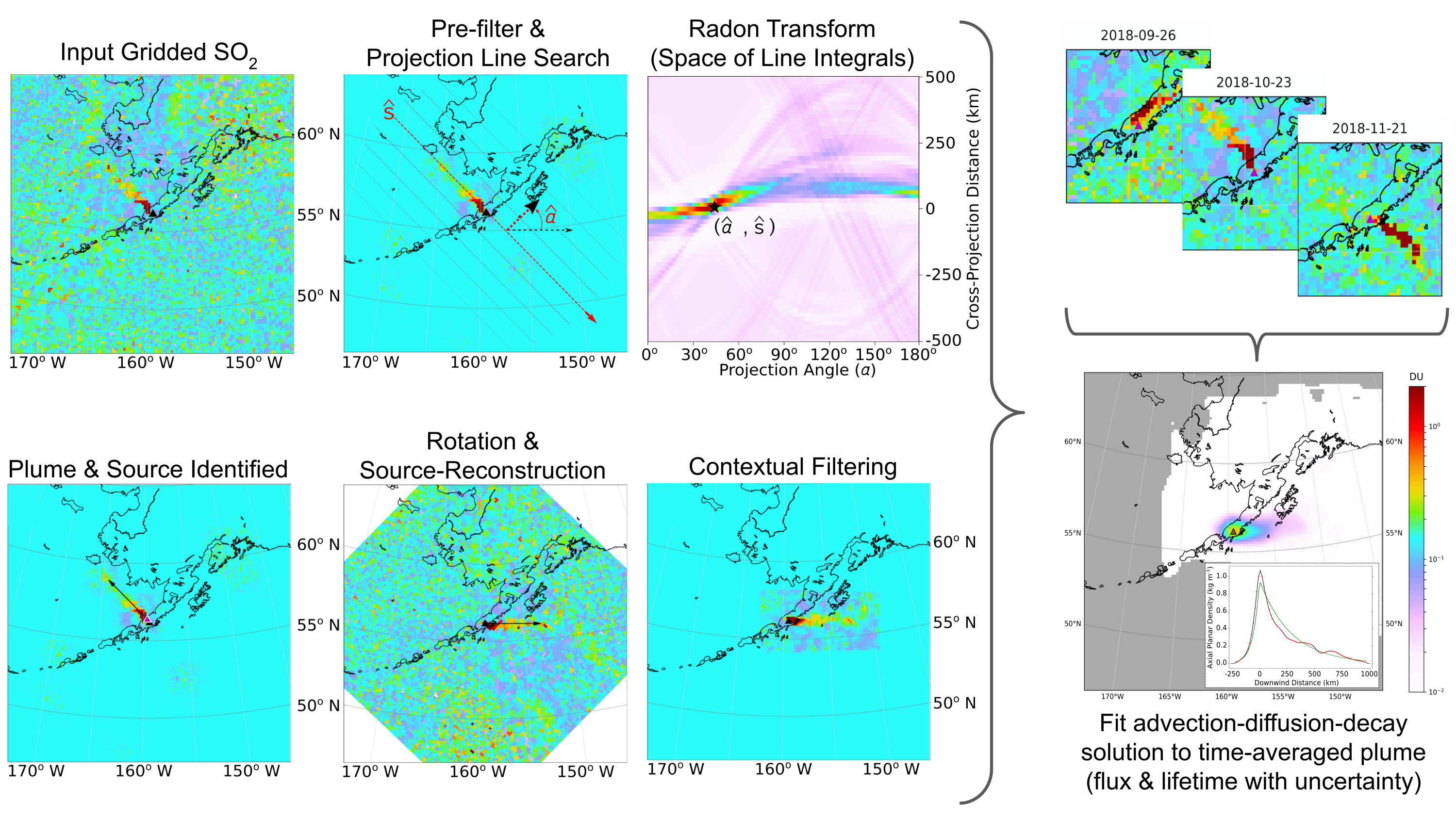
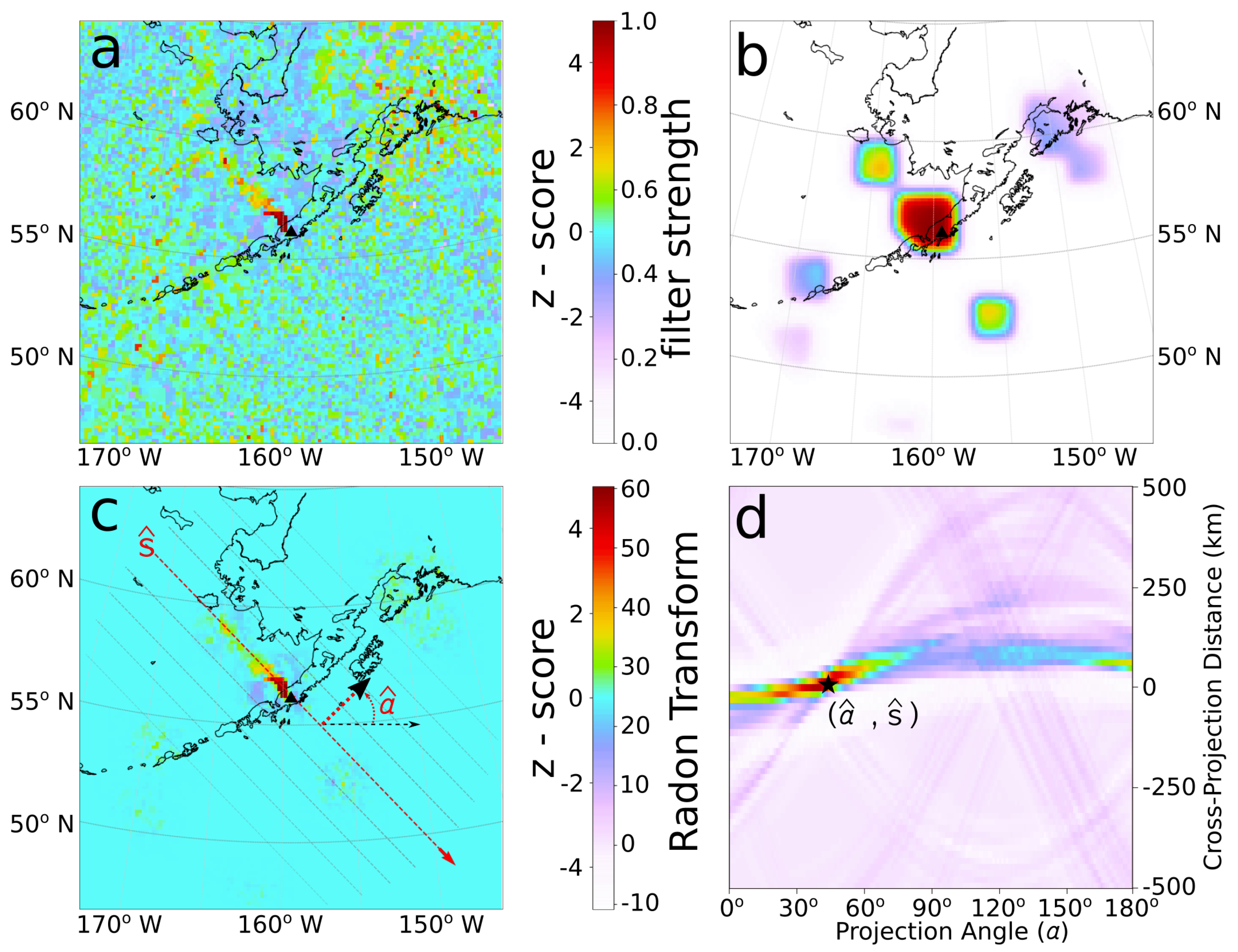
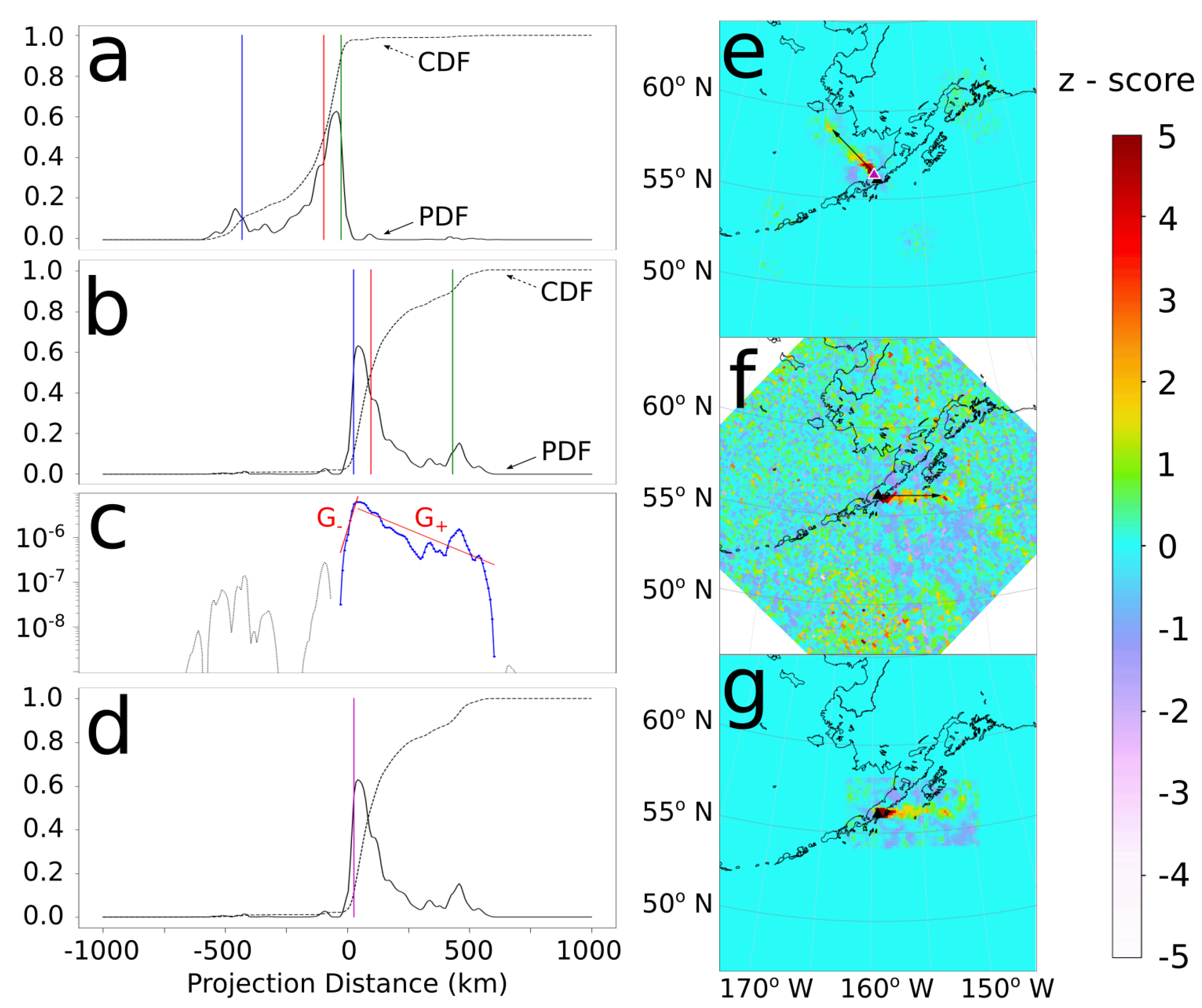
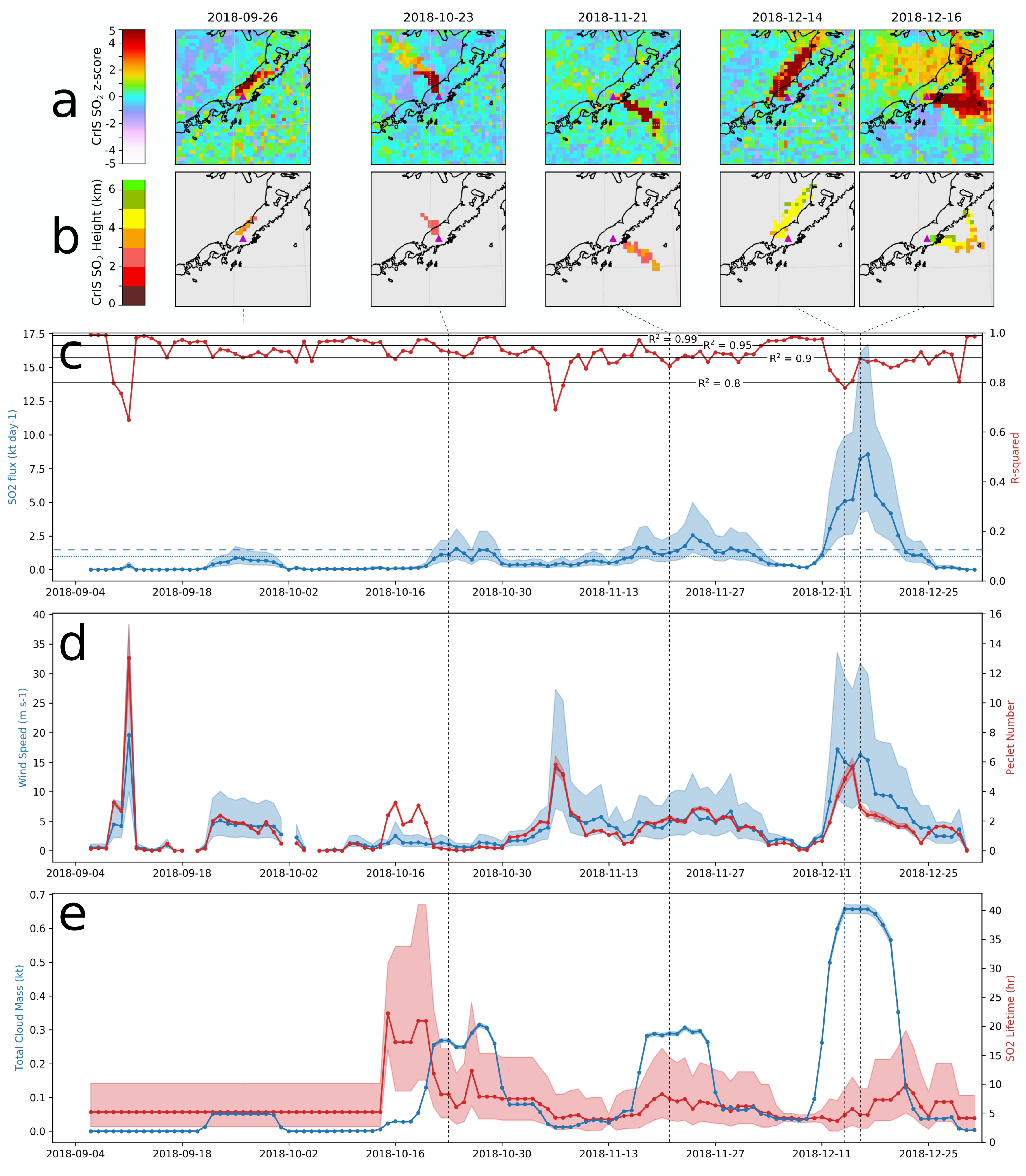
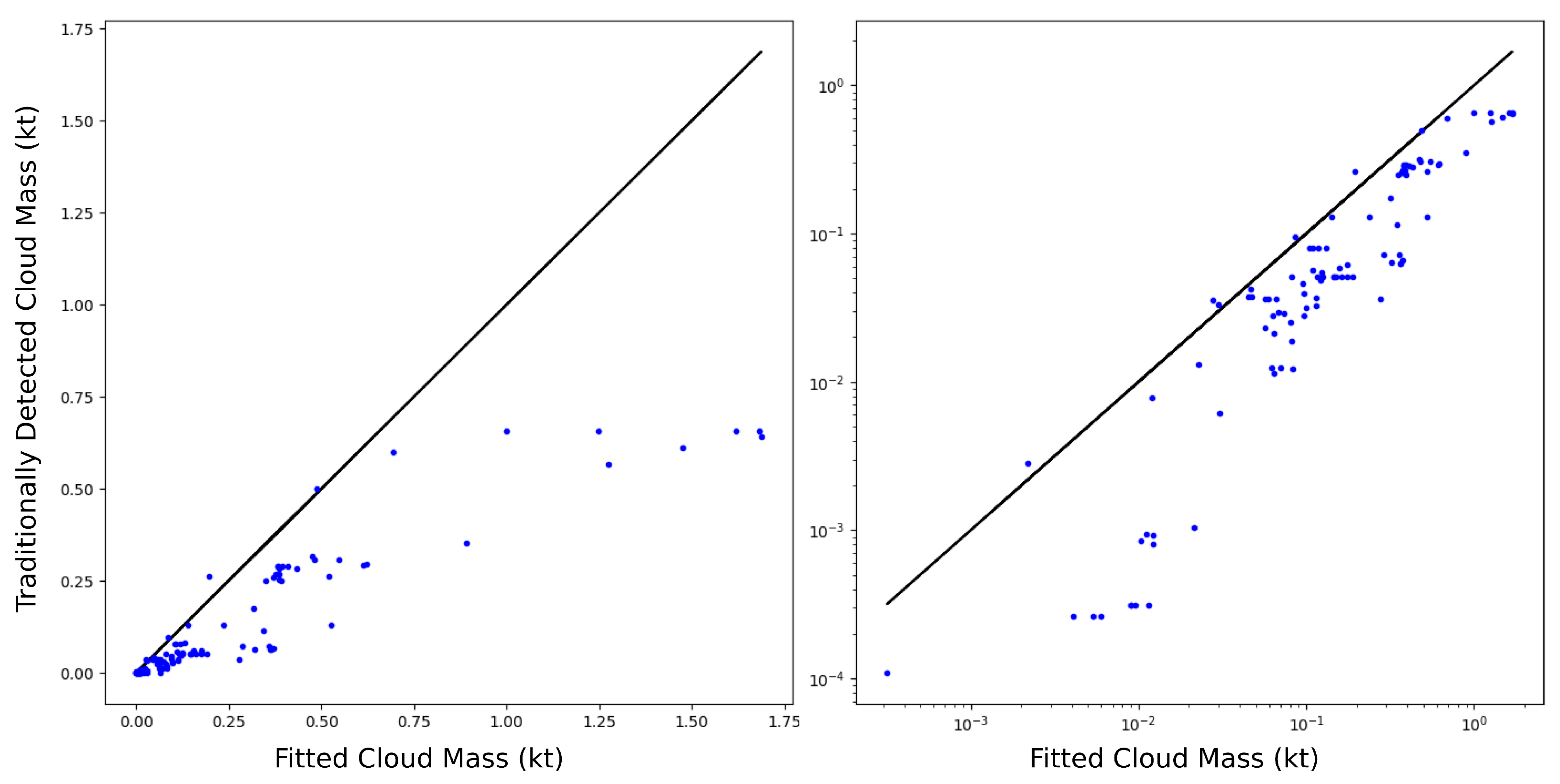
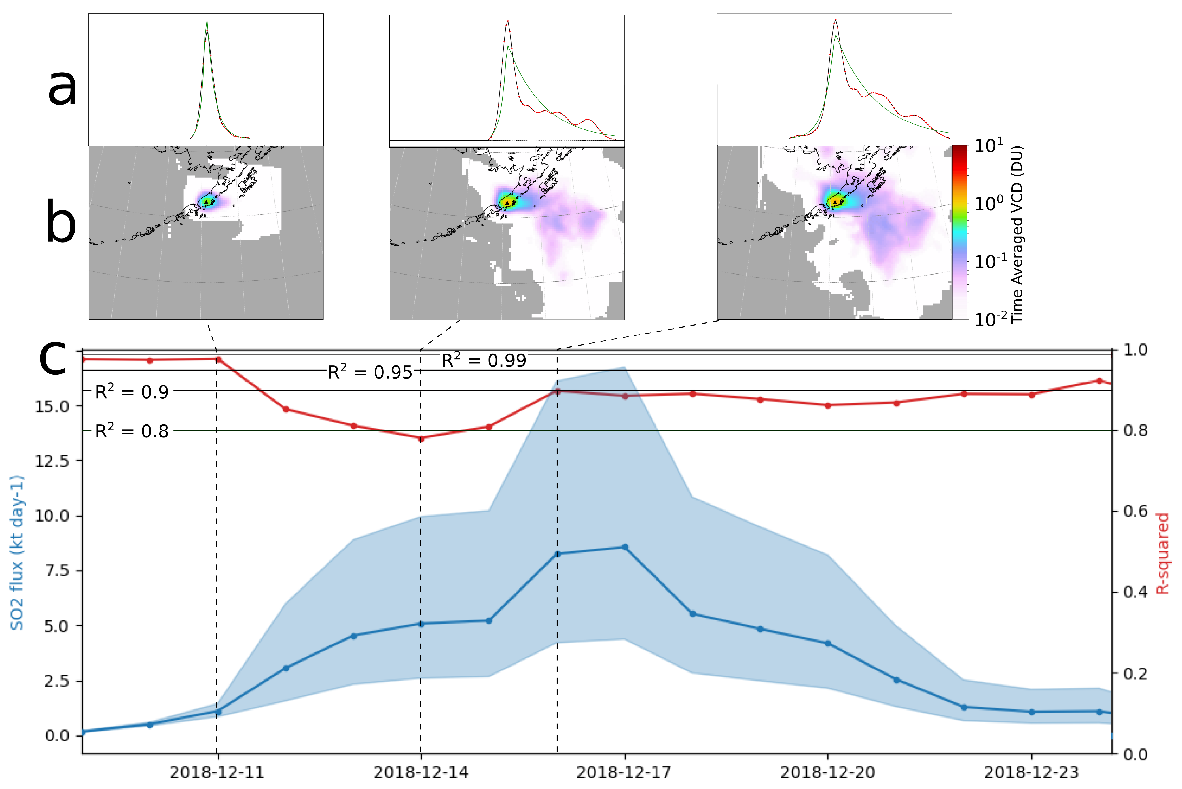
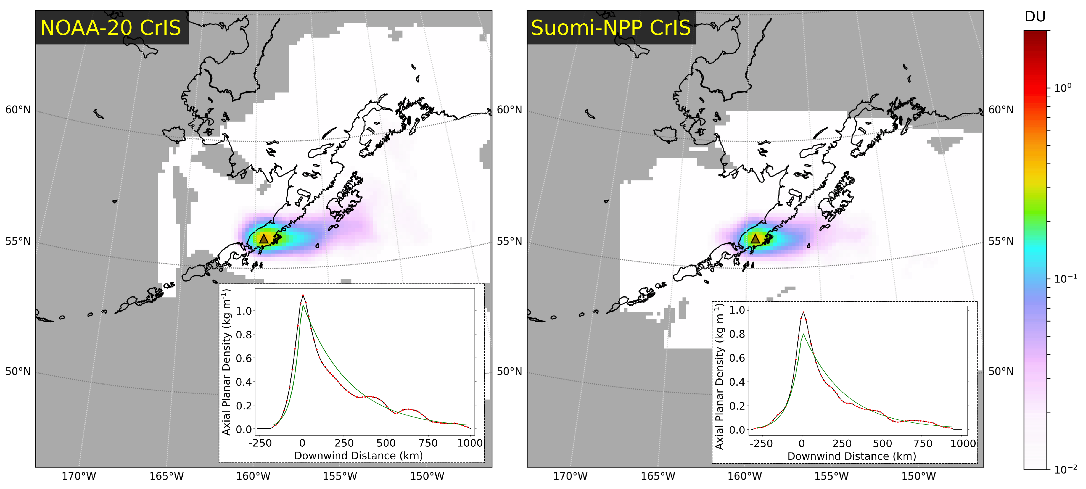
Table 1.
Time-averaged quantities with uncertainty from fitting: 1 September–31 December 2018, Veniaminof volcano.
Table 1.
Time-averaged quantities with uncertainty from fitting: 1 September–31 December 2018, Veniaminof volcano.
| Parameter | Units | Median | [5th, 95th] Percentiles |
|---|---|---|---|
| Flux | kt day | 1.5 | [0.8, 2.9] |
| wind speed | m s | 12.0 | [6.1, 23.4] |
| Eddy Diffusivity (downwind) | m s | 8.2 × 10 | [4.2,16.0] × 10 |
| Eddy Diffusivity (crosswind) | m s | 5.5 × 10 | [2.8, 10.8] × 10 |
| lifetime | h | 5.3 | [2.7, 10.4] |
| Plume Peclet Number | - | 3.4 | [3.2, 3.5] |
Table 2.
Fitting results for NOAA-20 and SNPP-only time-averaging: 1 September–31 December 2018, Veniaminof volcano.
Table 2.
Fitting results for NOAA-20 and SNPP-only time-averaging: 1 September–31 December 2018, Veniaminof volcano.
| Parameter | Units | Percentiles: Median [5th, 95th] | |
|---|---|---|---|
| NOAA-20 Only | SNPP Only | ||
| Flux | kt day | 1.6 [0.8, 3.2] | 1.0 [0.5, 2.0] |
| wind speed | m s | 12.5 [6.4, 24.4] | 8.1 [4.1, 15.8] |
| Eddy Diffusivity (downwind) | m s | 7.2 [3.7, 14.0] × 10 | 7.7 [4.0, 15.2] ×10 |
| Eddy Diffusivity (crosswind) | m s | 2.6 [1.4, 5.2] × 10 | 2.2 [1.1, 4.3] ×10 |
| lifetime | h | 5.1 [2.6, 10.0] | 6.6 [3.4, 12.9] |
| Plume Peclet Number | - | 4.0 [3.8, 4.2] | 2.0 [1.9, 2.1] |
Publisher’s Note: MDPI stays neutral with regard to jurisdictional claims in published maps and institutional affiliations. |
© 2021 by the authors. Licensee MDPI, Basel, Switzerland. This article is an open access article distributed under the terms and conditions of the Creative Commons Attribution (CC BY) license (http://creativecommons.org/licenses/by/4.0/).
Share and Cite
MDPI and ACS Style
Hyman, D.M.R.; Pavolonis, M.J.; Sieglaff, J. A Novel Approach to Estimating Time-Averaged Volcanic SO2 Fluxes from Infrared Satellite Measurements. Remote Sens. 2021, 13, 966. https://0-doi-org.brum.beds.ac.uk/10.3390/rs13050966
AMA Style
Hyman DMR, Pavolonis MJ, Sieglaff J. A Novel Approach to Estimating Time-Averaged Volcanic SO2 Fluxes from Infrared Satellite Measurements. Remote Sensing. 2021; 13(5):966. https://0-doi-org.brum.beds.ac.uk/10.3390/rs13050966
Chicago/Turabian StyleHyman, David M.R., Michael J. Pavolonis, and Justin Sieglaff. 2021. "A Novel Approach to Estimating Time-Averaged Volcanic SO2 Fluxes from Infrared Satellite Measurements" Remote Sensing 13, no. 5: 966. https://0-doi-org.brum.beds.ac.uk/10.3390/rs13050966
Note that from the first issue of 2016, this journal uses article numbers instead of page numbers. See further details here.