
Benchmarking Deep Learning Models for Cloud Detection in Landsat-8 and Sentinel-2 Images


Image Processing Laboratory, University of Valencia, 46980 Valencia, Spain
*
Author to whom correspondence should be addressed.
Remote Sens. 2021, 13(5), 992; https://0-doi-org.brum.beds.ac.uk/10.3390/rs13050992
Submission received: 4 February 2021
/
Revised: 27 February 2021
/
Accepted: 1 March 2021
/
Published: 5 March 2021
(This article belongs to the Special Issue Deep Learning-Based Cloud Detection for Remote Sensing Images)
Abstract
:The systematic monitoring of the Earth using optical satellites is limited by the presence of clouds. Accurately detecting these clouds is necessary to exploit satellite image archives in remote sensing applications. Despite many developments, cloud detection remains an unsolved problem with room for improvement, especially over bright surfaces and thin clouds. Recently, advances in cloud masking using deep learning have shown significant boosts in cloud detection accuracy. However, these works are validated in heterogeneous manners, and the comparison with operational threshold-based schemes is not consistent among many of them. In this work, we systematically compare deep learning models trained on Landsat-8 images on different Landsat-8 and Sentinel-2 publicly available datasets. Overall, we show that deep learning models exhibit a high detection accuracy when trained and tested on independent images from the same Landsat-8 dataset (intra-dataset validation), outperforming operational algorithms. However, the performance of deep learning models is similar to operational threshold-based ones when they are tested on different datasets of Landsat-8 images (inter-dataset validation) or datasets from a different sensor with similar radiometric characteristics such as Sentinel-2 (cross-sensor validation). The results suggest that (i) the development of cloud detection methods for new satellites can be based on deep learning models trained on data from similar sensors and (ii) there is a strong dependence of deep learning models on the dataset used for training and testing, which highlights the necessity of standardized datasets and procedures for benchmarking cloud detection models in the future.
1. Introduction
Earth observation data provided by remote sensing (RS) satellites enable the systematic monitoring of the Earth system as never before. Proof of this is the number of applications that use remote sensing data for crop yield estimation [1], biophysical parameter retrieval [2], damage assessment after natural disasters [3], or urban growth monitoring [4], among others. In most of these applications relying on optical sensors, the presence of clouds is a limitation that hampers the exploitation of the measured signal [5]. Hence, cloud detection is a required step in the processing chain of those RS products that will critically compromise their final quality.
Methodologies for cloud detection in multispectral images range from rule-based or thresholding approaches to advanced machine learning approaches. On the one hand, rule-based approaches exploit the physical properties of clouds that can be extracted from the reflectance on the different spectral bands of the image. Those properties are usually condensed in spectral indexes, which are then combined with a set of fixed or dynamic thresholds to produce a cloud mask. FMask [6] and Sen2Cor [7] are some relevant examples of these approaches, which are operationally implemented and their cloud masks are distributed together with Landsat and Sentinel-2 images, respectively. On the other hand, supervised machine learning (ML) approaches tackle cloud detection as a statistical classification problem where the cloud detection model is learned from a set of manually annotated images. Among ML approaches, there has recently been a burst of works in the literature using deep neural networks for cloud detection [8,9,10,11,12,13,14,15]. In particular, these works use fully convolutional neural networks (FCNNs) trained in a supervised manner using large manually annotated datasets of satellite images and cloud masks. These works show better performance compared with operational rule-based approaches; however; they are validated in heterogeneous ways, which makes their inter-comparison difficult.
In both cases, rule-based or ML-based cloud detection, the development of cloud detection models requires benchmarks to compare their performance and find areas of improvement. In order to benchmark cloud detection models, a representative set of pixels within the satellite images must be labeled as cloudy or cloud free. It is worth noting that, in cloud detection problems, the generation of a ground truth for a given image is a difficult task, since collecting simultaneous and collocated in situ measurements by ground stations is not feasible given the complex nature of clouds. Therefore, the golden standard in cloud detection usually consists of the manual labeling of image pixels by photo-interpretation. This task is generally time consuming, and for this reason, public labeled datasets are scarce for most recent sensors. In this context, the European Space Agency (ESA) and the National Aeronautics and Space Administration (NASA) have recently started the Cloud Masking Inter-comparison eXercise (CMIX) [16,17]. This international ESA-NASA collaborative initiative aims to benchmark current cloud detection models in images from Landsat-8 and Sentinel-2. For these two particular satellites, there exist several public manually annotated datasets with pairs of satellite images and ground truth cloud masks created by different research groups and institutions, such as: the Biome dataset [18], the Spatial Procedures for Automated Removal of Cloud and Shadow (SPARCS) dataset [19], or the 38-Clouds dataset [20] for Landsat-8 and the Hollstein dataset [21] or the recently published Bahetens-Hagolledataset [22] for Sentinel-2. Nevertheless, benchmarking cloud detection models in all these datasets is challenging because of the different formats and characteristics of the ground truth mask and also because there are inconsistencies in the cloud class definition, which is especially true for very thin clouds, cirrus clouds, and cloud borders.
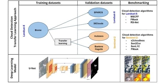
In this work, using the aforementioned datasets, we conduct an extensive and rigorous benchmark of deep learning models against several available open cloud detection methodologies. Specifically, first, we train deep learning models on Landsat-8 data and then: (i) we conduct intra- and inter-datasets validations using public Landsat-8 datasets; (ii) we test cross-sensor generalization of those models using Sentinel-2 public annotated data for validation; (iii) we compare our results with different operational and open-source cloud detection models; and (iv) we study the errors in challenging cases, such as thin clouds and cloud borders, and provide recommendations. Overall, our results show that, on the one hand, deep learning models have very good performance when tested on independent images from the same dataset (intra-dataset); on the other hand, they have similar performance as state-of-the-art threshold-based cloud detection methods when tested on different datasets (inter-datasets) from the same (Landsat-8) or similar (Sentinel-2) sensors. In our view, two conclusions arise from the obtained results: firstly, there is a strong model dependence on the labeling procedure used to create the ground truth dataset; secondly, models trained on Landsat-8 data transfer well to Sentinel-2. These results are aligned with previous work on transfer learning from Landsat-8 to Proba-V [15], which shows a clear path for developing ML-based cloud detection models for new satellites where no archive data are available for training.
Recent studies have compared the performance of different cloud detection algorithms for both Landsat [18] and Sentinel-2 [23,24]. Our work differs from those in several aspects: they are mainly focused on rule-based methods; they do not explicitly include the characteristics of the employed datasets in the validation analysis; and they do not consider cloud detection from a cross-sensor perspective, where developments from both satellites can help each other.
The rest of the paper is organized as follows. In Section 2, we describe the cloud detection methods used operationally in the Landsat and Sentinel-2 missions, which are used as the benchmark. In Section 3, the publicly available manually annotated datasets are described. In Section 4, we introduce the use of deep learning models for cloud detection and present the proposed model and transfer learning approach from Landsat-8 to Sentinel-2. Section 5 presents the results of the study. Finally, Section 6 discusses those results and provides our conclusions and recommendations.
2. Available Reference Algorithms for Cloud Detection
In this section, we describe the cloud detection methods used operationally in the Landsat-8 and Sentinel-2 missions. These methods are used (cf. Section 5) as a benchmark to assess the proposed deep learning-based methods.
The Function of Mask (FMask) algorithm [25] is the operational and most well-known cloud detection method for Landsat satellites. FMask is an automatic single-scene algorithm for detecting clouds and cloud shadows based on the application of thematic probability thresholds over top-of-atmosphere reflectance bands. These thresholds are based on physical properties of clouds, such as “whiteness”, “flatness”, or “temperature”; and the cloud shadows are detected taking into account the known sensor and solar geometry through the matching of geometric relationships with clouds. Over time, improvements have been made to mitigate the production of a high rate of false positives by means of filters, outlier detection, and the selection of potential cloud pixels [6,26,27].
For Sentinel-2, the operational cloud detection method is included in the ESA Sen2Cor processor [7]. Sen2Cor performs several tasks on Level 1C images such as atmospheric correction, retrievals of aerosol optical thickness and water vapor, cloud and snow uncertainty quantification, and scene classification. From the latter, available at 20 and 60 m resolution, a binary cloud mask can be inferred by merging the 11 possible classification labels (excluding defective pixels) into two categories: (1) land cover types (vegetation, not vegetated, dark area pixels, unclassified, water, snow, and cloud shadows), labeled as clear; and (2) cloud types (thin cirrus, cloud medium, and cloud high probability), labeled as cloud.
Two additional open source cloud detection methods are available for Sentinel-2. On the one hand, the FMask algorithm has been adapted for Sentinel-2 and was recently improved in [26] (Latest version available at http://www.pythonfmask.org/ (accessed on 3 February 2021)). On the other hand, the s2cloudless [28] algorithm, implemented in Sentinel-Hub (https://www.sentinel-hub.com (accessed on 3 February 2021)), is an ML-based approach for cloud detection. In particular, s2cloudless is a single-scene pixel-based classification method based on gradient boosting trees [29,30], which is trained on Sentinel-2 images using as the ground truth the cloud mask produced by the MAJAmultitemporal cloud detection method [31]. This model was validated over the S2-Hollstein dataset [32].
3. Labeled Datasets for Landsat-8 and Sentinel-2
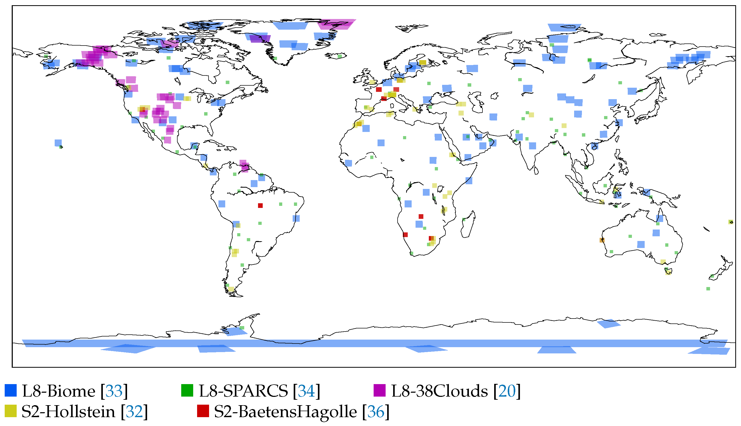
Manually labeled cloud masks are the golden standard to evaluate the performance of cloud detection algorithms in most satellite images. In this work, we exploit all (to our knowledge) publicly accessible manually labeled datasets for Landsat-8 and Sentinel-2. Figure 1 and Table 1 show the location and statistics of the employed datasets for both satellites. The reason to use all these datasets is two-fold: Firstly, we need labeled datasets to train our supervised neural network models in a wide and heterogeneous corpus of images. This is required to make our models robust across different land cover types, geographic locations, and seasons. Secondly, we take advantage of the datasets not used for training to benchmark our models against the reference cloud detection algorithms (explained in Section 2) and other deep learning-based models, when possible. Our purpose is to validate our method on images not only from different acquisitions, but also across different sensors (Sentinel-2 and Landsat-8) and using manually labeled images generated by different teams following different procedures.
- The L8-Biome dataset [33] consists of 96 Landsat-8 products [18]. In this dataset, the full scene is labeled in three different classes: Cloud, thin cloud, and clear. We merged the two cloud types into a single class in order to obtain a binary cloud mask. The satellite images have around 8000 × 8000 pixels and cover different locations around the Earth representing the eight major biomes.
- The L8-SPARCS dataset [34] was created for the validation of the cloud detection approach proposed in [19]. It consists of 80 Landsat-8 sub-scenes manually labeled in five different classes: Cloud, cloud-shadow, snow/ice, water, flooded, and clear-sky. In this work, we merge all the non-cloud classes in the class clear. The size of each sub-scene is 1000 × 1000 pixels; therefore, the amount of data of the L8-SPARCS dataset is much lower compared with the L8-Biome dataset.
- The L8-38Clouds dataset [20] consists of 38 Landsat-8 acquisitions. Each image includes the corresponding generated ground truth that uses the Landsat QA band (FMask) as the starting point. The current dataset corresponds to a refined version of a previous version generated by the same authors [35] with several modifications: (1) replacement of five images because of inaccuracies in the ground truth; (2) improvement of the training set through a manual labeling task carried out by the authors. It is worth noting that all acquisitions are from Central and North America, and most of the scenes are concentrated in the west-central part of the United States and Canada.
- The S2-Hollstein dataset [32] is a labeled set of 2.51 millions of pixels divided into six categories: Cloud, cirrus, snow/ice, shadow, water, and clear sky. Each category was analyzed individually on a wide spectral, temporal, and spatial range of samples contained in hand-drawn polygons, from 59 scenes around the globe in order to capture the natural variability of the MSI observations. Sentinel-2 images have bands at several spatial resolutions, i.e., 10, 20, and 60 m, but all bands were spatially resampled to 20 m in order to allow multispectral analysis [21]. Moreover, since S2-Hollstein is a pixel-wise dataset, the locations on the map (Figure 1) reflect the original Sentinel-2 products that were labeled.
- The S2-BaetensHagolle dataset [22] consists of a relatively recent collection of 39 Sentinel-2 L1C scenes created to benchmark different cloud masking approaches on Sentinel-2 [36] (Four scenes were not available in the Copernicus Open Access Hub because they used an old naming convention prior to 6 December 2016. Therefore, the dataset used in this work contains 35 images). Thirty-two of those images cover 10 sites and were chosen to ensure a wide diversity of geographic locations and a variety of atmospheric conditions, types of clouds, and land covers. The remaining seven scenes were taken from products used in the S2-Hollstein dataset in order to compare the quality of the generated ground truth. The reference cloud masks were manually labeled using an active learning algorithm, which employs common rules and criteria based on prior knowledge about the physical characteristics of clouds. The authors highlighted the difficulty of distinguishing thin clouds from features such as aerosols or haze. The final ground truth classifies each pixel into six categories: lands, water, snow, high clouds, low clouds, and cloud shadows.
Finally, it is important to remark that the statistics shown in Table 1 and the spatial location of Figure 1 highlight that the amount of available data for Landsat-8 and its spatial variability is much larger than for Sentinel-2. For this reason, we decided to use only Landsat-8 data for training (L8-Biome dataset) and keep the Sentinel-2 datasets only for validation purposes.
4. Methodology
In this section, we first briefly explain fully convolutional neural networks (FCNNs) and their use in image segmentation. Afterwards, a comprehensive literature of deep learning methods applied to cloud detection is presented. This review focuses on Landsat-8 and Sentinel-2 and highlights the necessity of benchmarking the different models in a systematic way. In Section 4.3, we categorize the different validation approaches followed in the literature depending on the datasets used for training and validation, i.e., intra-dataset, inter-dataset, and cross-sensor, since we will test our models in all the different modalities. Section 4.4 describes the neural network architectures chosen for this comparison. Section 4.5 explains how models trained on Landsat-8 are transferred to Sentinel-2 (cross-sensor transfer learning approach). Finally, Section 4.6 describes the performance metrics used in the results.
4.1. Fully Convolutional Neural Networks
Convolutional neural networks (CNNs) have shown a high performance in several supervised computer vision applications due to their ability to build complex mapping functions that exploit the spatial and spectral characteristics of an image in an end-to-end model. CNNs are built by stacking 2D convolutional filters, pointwise non-linear functions, and max-pooling operators to generate rich feature maps at multiple scale levels. The first CNNs were designed for image classification, where the goal was to provide the most likely category for an image over a set of categories. However, recently, there has been a significant upswing in the development of new methodologies to apply CNNs to other computer vision tasks such as image segmentation. This high performance associated with deep learning-based approaches is one of the main reasons for their popularity in many disciplines. However, there are some caveats: they highly rely on available training data; their increasing complexity may hamper their applicability when low inference times are required; and overfitting or underfitting issues may appear depending on the hyperparameters’ configuration. A plethora of different architectures can be found in the literature that try to find a trade-off between performance, robustness, and complexity for a particular application.
Fully convolutional neural networks (FCNN) [37] constitute the dominant approach for this problem currently. FCNNs are based only on convolutional operations, which make the networks applicable to images of arbitrary sizes with fast inference times. Fast inference times are critical for cloud detection since operational cloud masking algorithms are applied to every image acquisition of optical satellite instruments. Most FCNN architectures for image segmentation are based on encoder-decoder architectures, optionally adding skip-connections between encoder and decoder feature maps at some scales. In the decoder of those architectures, pooling operations are replaced by upsampling operations, such as interpolations or transpose convolutions [38], to produce output images with the same size as the inputs. One of the most used encoder-decoder FCNN architectures is U-Net, which was originally conceived of for medical image segmentation [39] and has been extensively applied in the remote sensing field [10,40].
4.2. Related Work on Deep Learning Models for Cloud Detection
In the literature, several approaches use modified versions of the U-Net architecture for cloud detection. The remote sensing network (RS-Net) [10] used a U-Net architecture to train different models on the L8-Biome and L8-SPARCS datasets, respectively. They validated their models on images of the same dataset and the opposite one (models trained on L8-Biome were tested on L8-SPARCS and vice versa), showing significant improvements over FMask, especially for snow/ice covers. Hughes and Kennedy [41] also trained and validated a U-Net using different images of the L8-SPARCS dataset, claiming an accuracy on par with human interpreters. Wieland et al. [40] also trained a U-Net on the L8-SPARCS dataset, which was validated on a custom private dataset of 14 1024 × 1024 Landsat-7, Landsat-8, and Sentinel-2 images. Zhang et al. designed a lightweight U-Net [14] targeting micro-satellites with limited processing resources. Their model was trained and validated on independent images from the L8-Biome dataset. Mohajerani et al. proposed an FCNN based on U-Net along with further modifications [20,35], which used only four input bands (RGBI). Their model was trained and validated in different images from the L8-38Clouds dataset showing a good trade-off between performance and efficiency with regard to the number of parameters and complexity compared to other deep learning architectures, also outperforming FMask. The authors in [11] used a different encoder-decoder architecture called SegNet [42], which was used to train models on the L7-Irish [43] and the L8-Biome datasets, respectively. The authors divided the images into patches, which were randomly split into training, validation, and test sets (i.e., the training and test datasets contained non-overlapping patches from the same image acquisitions). The resulting networks exhibited an outstanding accuracy compared to FMask on both Landsat-7 and Landsat-8 imagery. Li et al. [8] proposed a more complex encoder-decoder architecture called multi-scale feature extraction and feature fusion (MSCFF). They trained several networks with this architecture on the L7-Irish [43] dataset, the L8-Biome dataset, a public dataset of Gaofen-1 images, and high resolution labeled images exported from Google Earth, respectively. Each of these models were validated on independent images of the same dataset. In [9], the authors targeted cloud classification of image patches instead of image segmentation. The authors trained eight CNN ensembles consisting each of three deep network architectures (VGG-10, ResNet-50, and DenseNet-201) and the resulting combinations of training and testing with mixtures of three datasets from PlanetScope and Sentinel-2 sensors. Some combinations showed generalization over different sensors and geographic independence with performance comparable to the specific Sen2Cor [7] and the multisensor atmospheric correction and cloud screening (MACCS) [31] methods developed for Sentinel-2 mission images. In [44], an extended Hollstein dataset was used to compare ensembles of ML-based approaches, such as random forest and extra trees, CNN based on LeNet, and Sen2Cor. Finally, Mateo-Garcia et al. [15] trained cloud detection models independently on a dataset of Proba-V images and on L8-Biome. They tested the models trained using Landsat-8 on Proba-V images and models trained using Proba-V on Landsat-8. They showed very high detection accuracy despite differences in the spatial resolution and spectral response of the satellite instruments.
4.3. Validation Approaches
As can be observed in the previous section, proposals based on deep learning vary in terms of complexity, defined by the chosen architecture, and in terms of the data used for training and testing. These differences make it difficult to determine which approach leads to a better overall performance for Landsat-8 and Sentinel-2. In this work, we use the same architecture (Section 4.4), which we systematically test following three different training and testing approaches:
- Intra-dataset: Images and cloud masks from the same dataset are split into training and test subsets. This approach is perhaps the most common one. Methods using this validation scheme are trained and evaluated on a set of images acquired by the same sensor, and the corresponding ground truth is generated for all the images in the dataset following the same procedure, which involves aspects such as sampling and labeling criteria. In order to provide unbiased estimates, this train-test split should be done at the image acquisition level (i.e., training and test images should be from different acquisitions); otherwise, it is likely to incur an inflated cloud detection accuracy due to spatial correlations [45].
- Inter-dataset: Images and the ground truth in the training and test splits come from different datasets, but from the same sensor. Differences between the training and test data come now also from having ground truth masks labeled by different experts following different procedures.
- Cross-sensor: Images in the training and testing phases belong to different sensors. In this case, the input images are from different sensors, and usually, the ground truth is also derived by different teams following different methodologies. This type of transfer learning approach usually requires an additional step to adapt the image characteristics from one sensor to another [15,46].
Table 2 shows some of the most recent works on deep learning for cloud masking, applied to Landsat-8 and Sentinel-2 imagery, depending on the validation scheme used. The predominance of the intra-dataset scheme is notorious; The intra-dataset scheme tends to lead to a very high cloud detection accuracy and larger gains when compared with threshold-based methods [8,35,41]; however, in several cases, these models are trained on relatively small or local datasets (L8-SPARCS or L8-38Clouds), which might not be representative of global land cover and cloud conditions. One strategy to determine whether these models generalize to different conditions is to test them over independent datasets following an inter-dataset strategy. Works using an inter-dataset strategy are more scarce than the intra-dataset validation [10,40] and usually lead to a lower cloud detection accuracy. This could by caused by either a lack of a representative statistical sample of the training data or by differences or errors between the ground truth of the different datasets, which are usually caused by disagreements in very thin clouds and cloud borders. In Section 5, we test separately the accuracy of our models on thin and thick clouds and excluding the effects of cloud borders. Finally, very few works address cross-sensor validation [15,40] and none of them for public Sentinel-2 data, which is one of the contributions of our work.
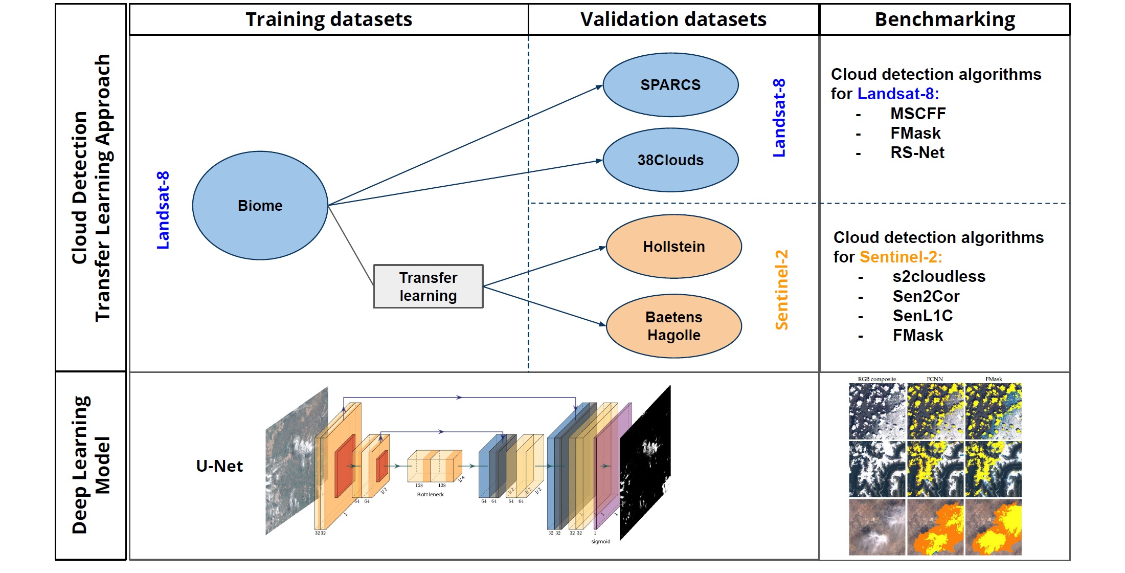
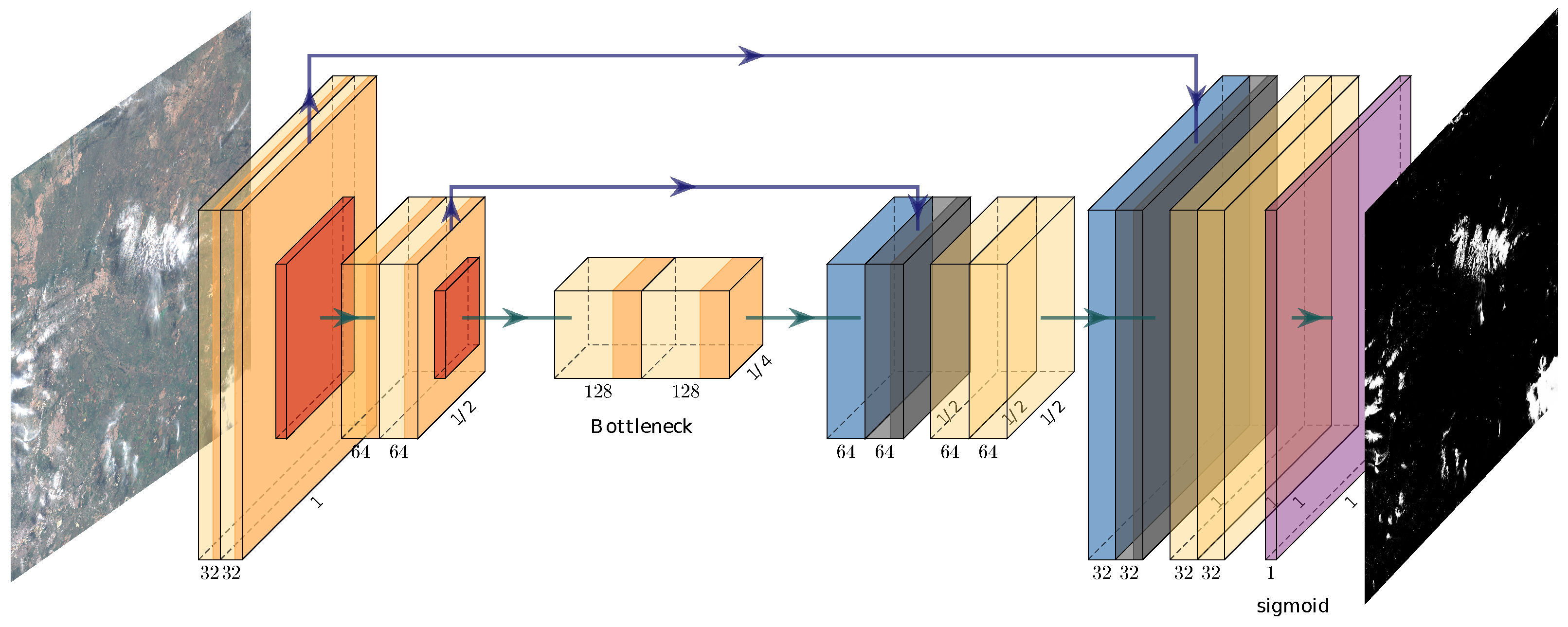
4.4. Proposed Deep Learning Model
In this work, we use a modified version of the U-Net architecture proposed by the authors in [15]. The proposed changes in the U-Net architecture seek to, on the one hand, speed up the training and testing process and, on the other hand, provide a simpler architecture that can be used as a baseline for future works. In particular, the proposed architecture has only two downsampling steps instead of the five of the original U-Net. We also reduced the amount of filters for each convolutional layer and replaced the convolutions with depthwise separable convolutions, which have significantly less trainable parameters. The detailed architecture is shown in Figure 2. It has approximately 96,000 trainable parameters, which is around 1% of the original U-Net parameters (7.8 million). In addition, it requires 2.18 M floating point operations (FLOPS) to compute the cloud mask of a 256 × 256 image patch, which is a reduction of around 92% compared with U-Net (interested readers can see the implementation at https://gist.github.com/gonzmg88/8a27dab653982817034938b0af1a2bf7 (accessed on 3 February 2021)). This is also 2.5% of the weights of the lightweight U-Net proposed in [14] and 20% of their FLOPS.
Networks were trained and tested using top of atmosphere (TOA) calibrated radiance as the input. In particular, we used Level 1TP Landsat-8 products and Level 1C Sentinel-2 products, respectively, converted to TOA reflectance using their corresponding calibration factors available in the metadata of the image. These TOA reflectance inputs were further normalized using the mean and standard deviation from the L8-Biome dataset for each band in order to better condition the training of the networks. In our experiments, we trained the networks from scratch to minimize the pixelwise binary cross-entropy between the model predictions and the ground truth labels. In particular, we cropped the images in overlapping patches of 32 × 32 pixels, then random batches of 64 patches were formed to train the neural network using stochastic gradient descent. Networks were trained for 7.2 × optimization steps using the Adam [47] update of the weights with an initial learning rate of and a weight decay of 5 ×. The weights of the different layers of the networks were initialized using the defaults in the TensorFlow v2.1 framework [48].
We observed that the random initialization of the weights and the stochastic nature of the optimization process produced networks with a slightly different detection accuracy. In order to account for that uncertainty, in all our experiments, we trained 10 copies of the same model and report the standard deviation of the selected cloud detection metrics. This contrasts with most deep learning works in the literature that only report best case scenarios.
4.5. Transfer Learning Across Sensors
The publicly available datasets described in Section 3 for Sentinel-2 are not suitable for training FCNN deep learning models. This is because, in the case of the S2-BaetensHagolle dataset, it has limited spatial variability, as shown in Figure 1 (i.e., there are only 13 unique locations across the globe). In the case of the S2-Hollstein dataset, it does not have fully labeled scenes (only scattered isolated pixels), which limits the applicability of fully convolutional networks. Hence, in order to build an FCNN model for Sentinel-2, we rely on Landsat-8 data for training the models and then transfer them to Sentinel-2 data. This means that our approach to provide models for Landsat-8 and Sentinel-2 consists of training the FCNN using only Landsat-8 data. In particular, we trained our FCNNs using the L8-Biome dataset, which has the largest amount of data and was built to be representative of the different Earth ecosystems and cloud conditions [18].
In order to apply models trained on Landsat-8 data to Sentinel-2 images, we first must take into account the spatial and spectral characteristics of both sensors. Figure 3 shows the spatial resolution and the overlapping bands for Landsat-8 and Sentinel-2. As we can see, Landsat-8 and Sentinel-2 have several overlapping bands in the visible, near-infrared (NIR), and short-wave infrared (SWIR) part of the spectra. Hence, our models will be restricted to use as the inputs in Landsat-8 only the bands that are also available in Sentinel-2. In this work, we used two band configurations denoted by and . In the band configuration, we used a reduced set of 4 bands consisting of visible bands (blue, green, and red) combined with the near-infrared band (Bands B2, B3, B4, and B5 of Landsat-8 and Bands B2, B3, B4, and B8 of Sentinel-2). The band configuration increased the set of bands by adding SWIR1 and SWIR2 (Bands B6 and B7 in Landsat-8 and Bands B11 and B12 in Sentinel-2). Regarding the spatial resolution, we simply resampled the Sentinel-2 bands to 30 m resolution by cubic-spline interpolation before applying the model. The assessment with the ground truth was done at 30 m resolution as well. Finally, it is important to point out again that the input of the network was expected to be top-of-atmosphere (TOA) reflectance generated using the correction factors available in the image product metadata (Sentinel-2 Level 1C products).
A Python implementation of the proposed cloud detection algorithm is provided in a public repository (https://github.com/IPL-UV/DL-L8S2-UV (accessed on 3 February 2021)) in order to allow the community to compare the proposed transfer models for both Landsat-8 and Sentinel-2 images.
4.6. Performance Metrics
In order to benchmark the different models, we used standard metrics for classification such as overall accuracy (OA), commission error (CE), interpreted as cloud prediction when the ground truth indicates a clear pixel, and omission error (OE), i.e., clear prediction when the ground truth indicates a cloud pixel. Those metrics were computed from the confusion matrix over all valid pixels across all images in the dataset. This contrasts with the approach followed in some works that compute metrics for each image and later average the results. It is well known that the OA might be biased when the dataset is not balanced (very different proportions of cloud and clear pixels); however, the datasets that we considered have relatively similar proportions of clear and cloudy pixels (see Table 1). We experimented with the and Cohen’s kappa statistics, but overall, they exhibited the same patterns and trends as OA; hence, we do not report them for simplicity.
5. Experimental Results
In this section, we present first the intra-dataset experiments where some images of the L8-Biome dataset are used for training and others for testing following the same train-test split used in [8]. Secondly, in Section 5.2, we discuss the inter-dataset experiments where the models trained in the full L8-Biome dataset are tested in other Landsat-8 datasets (L8-SPARCS and L8-38Clouds). Section 5.3 contains the cross-sensor transfer learning experiments where the previous models (trained in the complete L8-Biome dataset) are evaluated in the Sentinel-2 datasets, as explained in Section 4.5. In particular, in this case, we take advantage of the fine-level details of the annotations of those datasets to report independent results for both thin and thick clouds. Finally, in Section 5.4, we analyze how the spatial post-processing of the ground truth over cloud masks borders impacts the detection accuracy of the different models.
5.1. Landsat-8 Cloud Detection Intra-Dataset Results
For the intra-dataset experiments, we trained our FCNN models on the L8-Biome dataset using the same 73 acquisitions as in [8]. Therefore, data were split in a proportion of of images for training and for testing. Our models were trained with different band combinations to compare with [8]: VNIR bands (visible bands + NIR), SWIR bands (visible bands + NIR + SWIR bands), and ALLbands (i.e., all Landsat-8 bands except panchromatic). Afterwards, those models were tested in 19 different images from the L8-Biome (the authors in [8] excluded four images from the L8-Biome dataset containing errors). As we explained in Section 4.4, we trained 10 copies of the network changing the random initialization of the weights and the stochastic nature of the optimization process. This is reflected in the value under parenthesis in the tables. Table 3 shows the averaged accuracy metrics over the 19 test images. We see that the overall accuracy consistently increases when more bands are used for training. In addition, we see that deep learning models outperform FMask by a large margin in all different configurations and that commission and omission errors are balanced (i.e., omission of clouds is as likely as classifying clear pixels as cloudy). Compared to the MSCFF networks [8], we see that our results are slightly worse, but within the obtained uncertainty levels. In fact, a drop in performance is expected since our networks have a significant lower complexity than MSCFF [8].
5.2. Landsat-8 Cloud Detection Inter-Dataset Results
For the inter-dataset experiments, models were trained and validated with different Landsat-8 datasets. In these experiments, we trained the models on the 96 images of the L8-Biome dataset (denoted as ) using two different input bands combinations: and . Afterwards, those models were tested on the L8-SPARCS and L8-38Clouds datasets and compared with the operational FMask and with RS-Net [10] when available (RS-Net was trained on the L8-Biome dataset and validated on the L8-SPARCS).
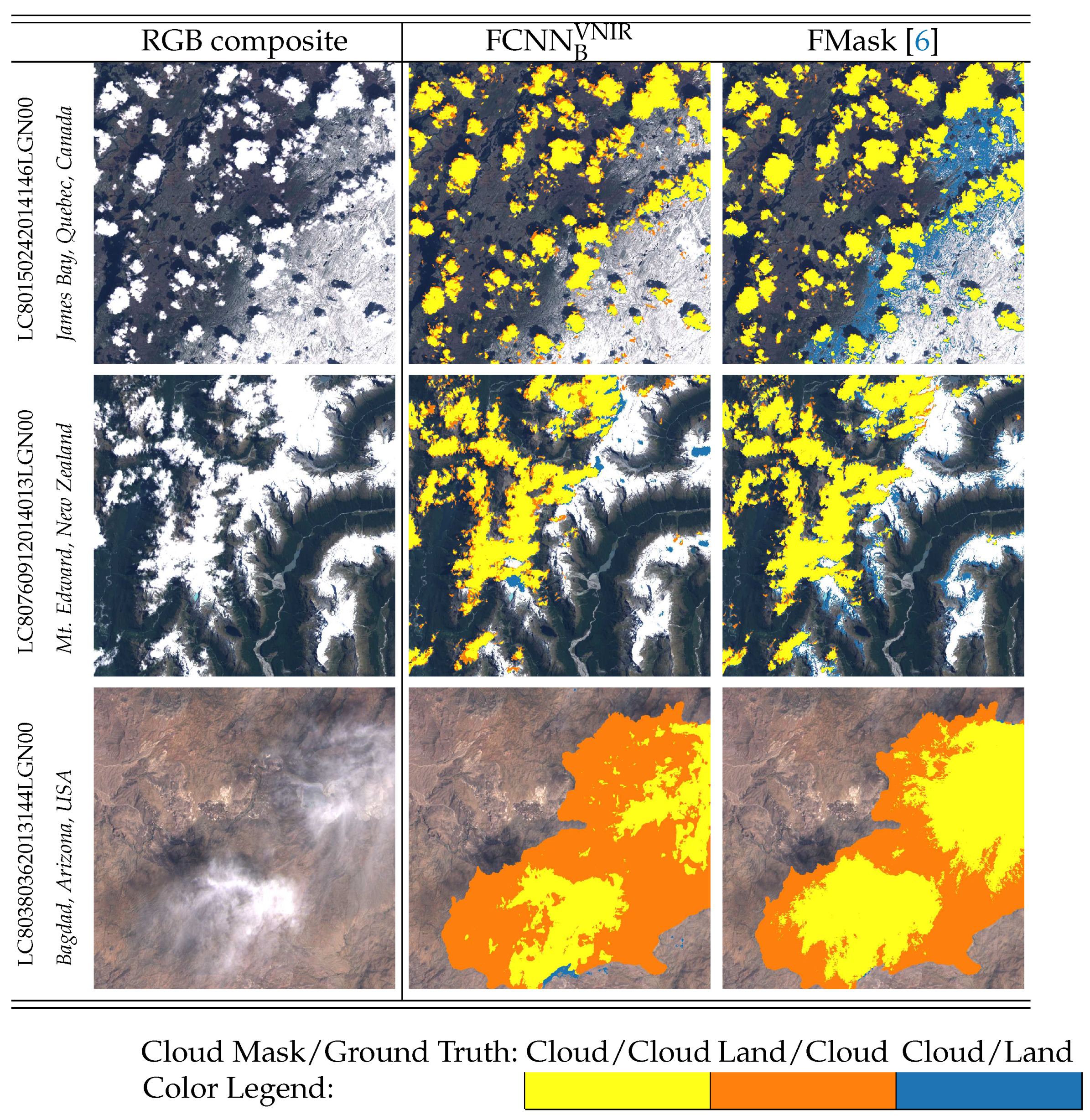
Table 4 shows the results in the L8-SPARCS dataset. We include the results of RS-Net using two different band configurations: ALL-NTconfiguration, i.e., all bands except thermal and panchromatic bands (which obtain the highest accuracy among all the models), and the VNIR configuration. Overall, we see that deep learning models obtain a high accuracy on par with FMask for models using the VNIR configuration and approximately one point higher for the models that use more bands. Among our developed models, yields improvements in terms of overall accuracy and commission error compared to . Besides, the standard deviation of the metrics of models trained with different random initialization is lower for the model. Similarly, RS-Net offers slightly better performance using ALL-NT over the VNIR band configuration. On the other hand, FMask shows slightly lower accuracy, but significantly reduces the omission errors. This might be due to the implementation of the method, which includes a morphological dilation step to spatially grow the produced cloud mask. Figure 4 shows some visual examples of the produced cloud masks compared with the L8-SPARCS ground truth. We see that FMask is more accurate in detecting the semi-transparent clouds in the third row. However, it shows a higher rate of commission errors in high reflective land cover types such as snow and mountains, which is clearly visible in the first and second row.
Table 5 shows the detection accuracy of the same models, and , on the L8-38Clouds dataset. We can see that there are significant differences between these results and the previous results on the L8-SPARCS dataset. Specifically, it can be noticed that models with more bands () obtain lower overall accuracy and higher omission error than models using less bands (). Nonetheless, the commission is reduced in both datasets with the SWIR configuration, albeit that the differences are not statistically significant. Perhaps the main point that we can draw from these two experiments is that using SWIR bands does not strictly imply a significant improvement in classification error. Finally, the results of the FMask on the L8-38Clouds dataset are much better than on the L8-SPARCS dataset. This is mainly because the L8-38Clouds ground truth was generated using the QA band (FMask) as the starting point. This shows the strong bias that each particular labeled dataset exhibits.
It is worth noting here that this inter-dataset validation of the FCNN models trained on L8-Biome against both the L8-SPARCS and L8-38Clouds datasets is justified by two facts. On the one hand, when comparing the properties of both datasets, it can be observed from Table 1 that the labels’ distribution in terms of the ratio of cloudy and clear pixels diverges, having a higher proportion of pixels labeled as cloud on L8-38Clouds. On the other hand, a limited number of acquired geographical locations can be observed in Figure 1 for L8-38Clouds, which a priori might be a drawback for a consistent validation due to the lower representativeness of possible natural scenarios.
5.3. Transfer Learning from Landsat-8 to Sentinel-2 for Cloud Detection
For evaluation of the Sentinel-2 data, we used the same trained models presented in the previous section: and . In order to test those models on Sentinel-2, we followed the transfer learning scheme described in Section 4.5: first, all Sentinel-2 input bands were resampled to Landsat-8 resolution (30 m); and the outputs and ground truth mask of every method were resampled to 30 m for consistency in the comparison. The cloud masks for comparison purposes were generated with the Sen2Cor v2.8 processor, Sentinel-2 FMask algorithm v0.5.4, the cloud mask distributed with the L1C Sentinel-2 products, and the s2cloudless algorithm v1.4.0, as described in Section 2. Results are stratified based on the thin and thick cloud labels available in the ground truth datasets: S2-BaetensHagolle and S2-Hollstein.
It is worth noting that thin clouds are usually more challenging to identify due to their intrinsic nature as a mixture of cloud and land/water spectra. This affects both the automatic cloud detection methods and the ground truth created by human photo-interpretation. Hence, we expect more disagreements between the models and the ground truth in pixels labeled as thin clouds.
The results on the S2-BaetensHagolle dataset are shown in Table 6. We can see that transferred models, and , exhibit a similar overall accuracy as in the L8-38Clouds evaluation when considering the thin cloud pixels.
On the one hand, the threshold-based methods tailored for Sentinel-2 data (Sen2Cor, SenL1C, and FMask) have relatively similar performance in terms of overall accuracy. These results highlight the capabilities of the transfer learning approach taking into account that the model is completely agnostic to Sentinel-2 images during the training phase. On the other hand, the s2cloudless algorithm significantly outperforms all the other methods. This can be explained by a well-executed training procedure in Sentinel-2 imagery, an exhaustive cross-validation, and the large amount of training pixels with a considerable diversity of tiles from the MAJA products.
If thin clouds, which are nearly half of the cloud labels, are excluded from the validation (right panel in Table 6), all methods get a substantial boost in terms of global performance. This improvement is especially noticeable in the transfer learning models with a reduction of the OE of around . The s2cloudless method also significantly reduces the OE. Threshold-based methods are less affected probably due to the over-masking caused by the morphological growth of the cloud masks.
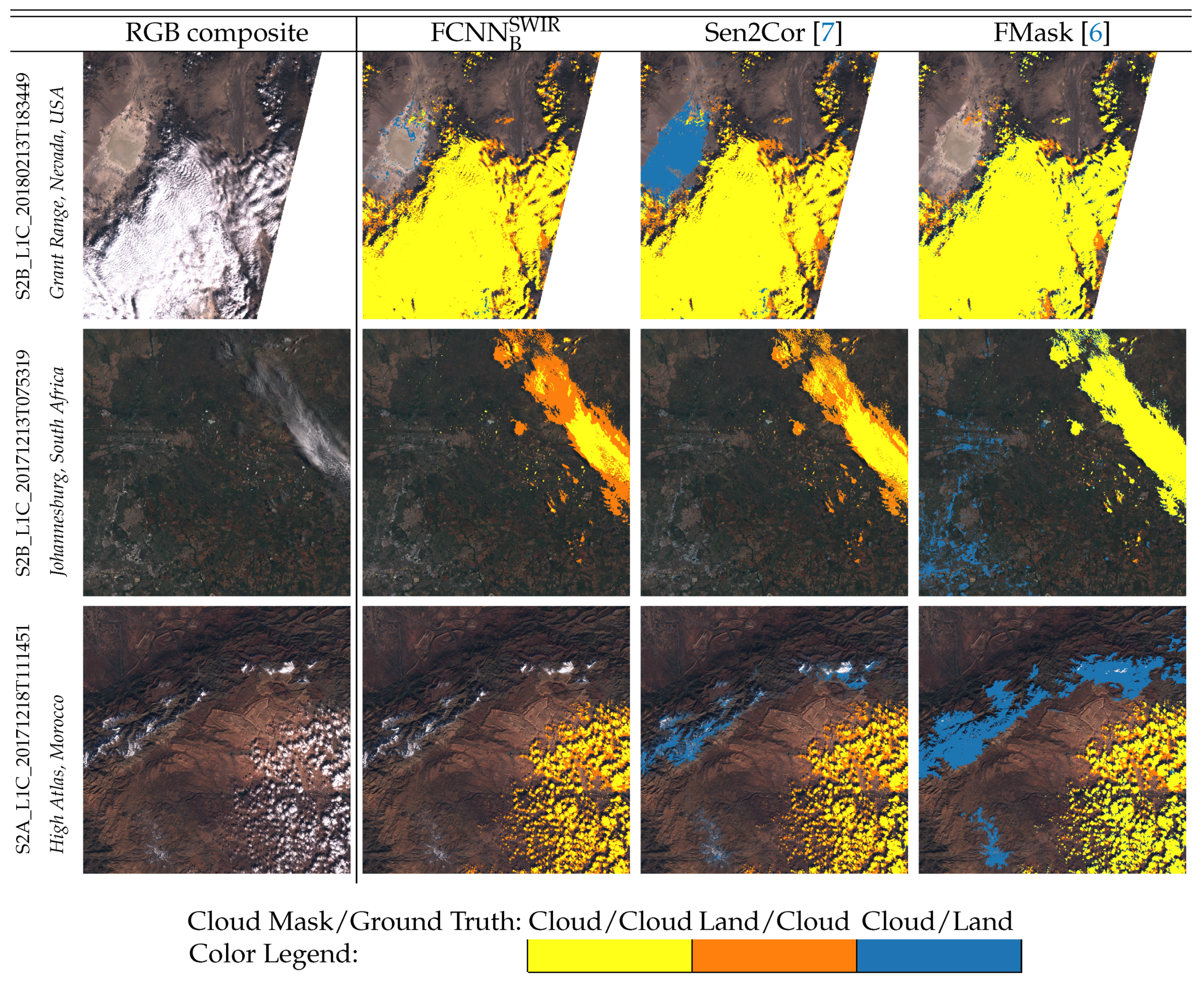
Figure 5 shows three scenes acquired over three different locations with different atmospheric, climatic, and seasonal conditions presenting different types of land covers and clouds. The benchmarked methods correctly detect most of the pixels affected by clouds, but they present different types of misclassifications over high reflectance pixels. In the first row, there are bright sand pixels that are incorrectly classified as clouds by the operational algorithm, Sen2Cor. The second row shows an acquisition of an urban area where some bright pixels are detected as cloud, increasing the FMask commission error. The third row shows a mountainous area with snow, where some pixels affected by snow present a high spectral response in the visible spectrum. These pixels are classified as clouds by the Sen2Cor and FMask methods. In this case, is able to correctly discriminate the problematic pixels and outperforms the previous algorithms through the transferred knowledge from Landsat-8. However, Sen2Cor and present a similar clear conservative behavior, and they do not effectively detect thin clouds around cloud borders. In general terms, one can observe an excellent performance of when classifying challenging areas with high reflectance surfaces. On the other hand, as was observed in Landsat-8 images, the FMask algorithm reduces the omission error due to an improved detection over thin clouds and to the intrinsic implementation of the spatial growth of the cloud mask edges.
Table 7 shows the evaluation of all the models in the S2-Hollstein dataset. This dataset has a similar proportion of thin clouds, thick clouds, and clear labels compared to the S2-BaetensHagolle dataset. In this case, the machine learning models exhibit larger gains compared with threshold-based methods in both thin and thick clouds (left panel) and thick clouds only (right panel). Additionally, by excluding the thin clouds in the validation, the reduction of the OE is very high in the ML-based models. In the case of s2cloudless, these good results can be also explained by the fact that the s2cloudless algorithm, although trained on MAJA products, was validated on the S2-Hollstein dataset. This supports the idea that proposed cloud detection algorithms tend to perform better on the datasets used by their authors to tune the models, suggesting somehow an overfitting at the dataset level.
5.4. Impact of Cloud Borders on the Cloud Detection Accuracy
In view of the results of the previous section, the performance of some algorithms is clearly biased depending on the dataset used for evaluation. The assumptions and choices made during the generation of the ground truth can critically affect the performance of an algorithm on a particular dataset. This is the case, for instance, of the L8-38Clouds dataset, which was created by manually refining the FMask cloud mask from the Landsat QA band. As a consequence, the FMask algorithm presented an overoptimistic performance on the L8-38Clouds dataset, as was shown in Section 5.2.
Another important factor affecting cloud detection accuracy is the performance of the algorithms over critical cloud detection problems, just because most errors and discrepancies occur on these pixels. Thin and semi-transparent clouds located on cloud borders are a clear example, since defining a binary class label in these mixed pixels is a difficult task. Therefore, the way in which these pixels are treated by either the ground truth or the cloud detection algorithm will significantly affect the cloud detection performance. The results excluding thin clouds from the ground truth in Section 5.3 showed significant differences between the developed machine learning models and the algorithms that include a spatial buffer to over-mask cloud borders. This issue was also highlighted in [24], where the authors verified that the analyzed cloud detection methods yielded different results because of different definitions of the dilation buffer size for the cloud masks.
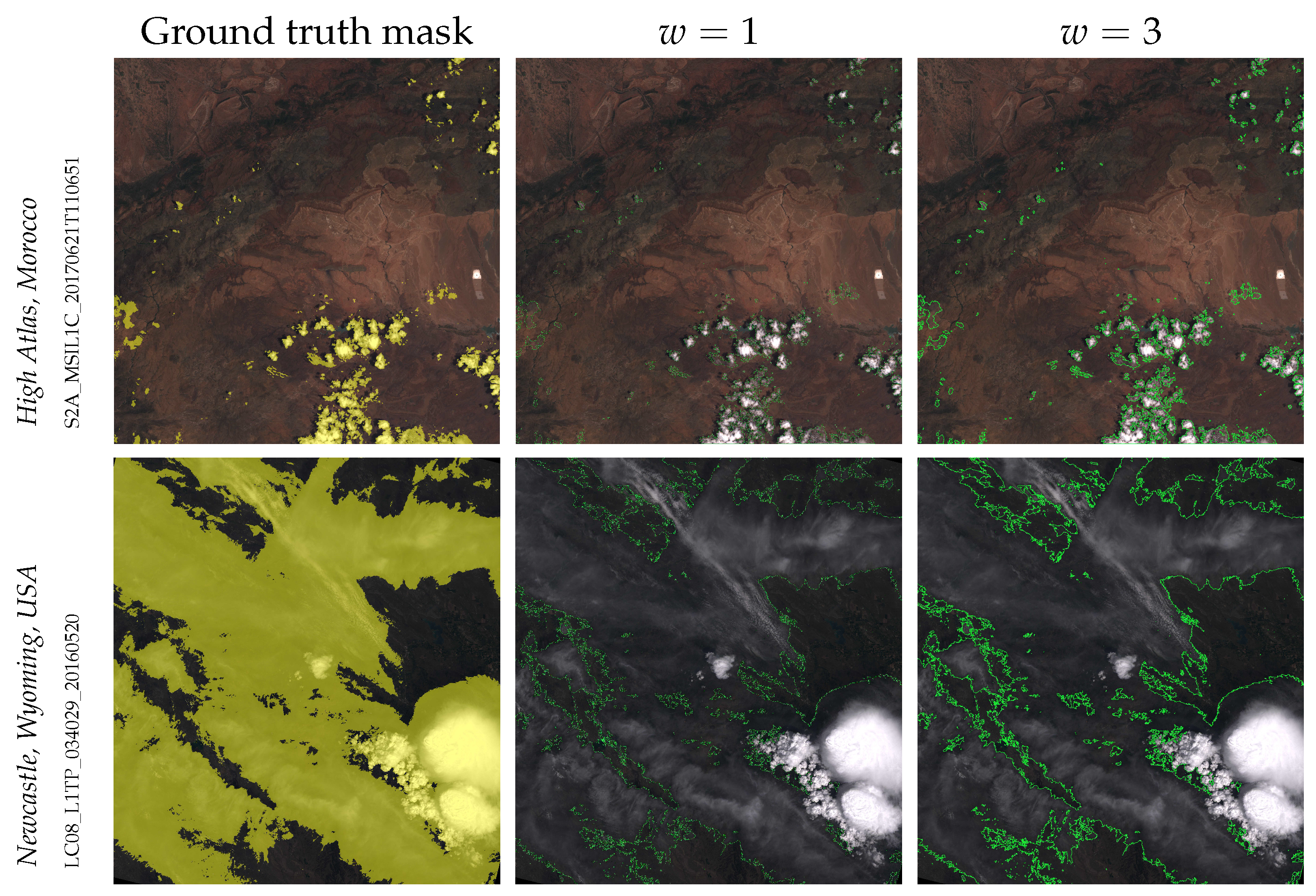
In this section, we analyze the impact of cloud borders on the cloud detection accuracy for all the cloud detection methods and for the different Landsat-8 and Sentinel-2 datasets. In order to quantify this effect, we exclude the pixels around the cloud mask edges of the ground truth from the computation of the performance metrics for the test images. In the experiments, we increasingly excluded a wider symmetric region around cloud edges to analyze the dependence on the buffer size. In particular, we excluded a number of pixels , in both the inward and outward direction from the cloud edges, by morphologically eroding and dilating the binary cloud masks. Figure 6 shows one example for Sentinel-2 and one for Landsat-8 where excluded pixels are highlighted in green around cloud edges. Only two w values are displayed in these examples for illustrative purposes.
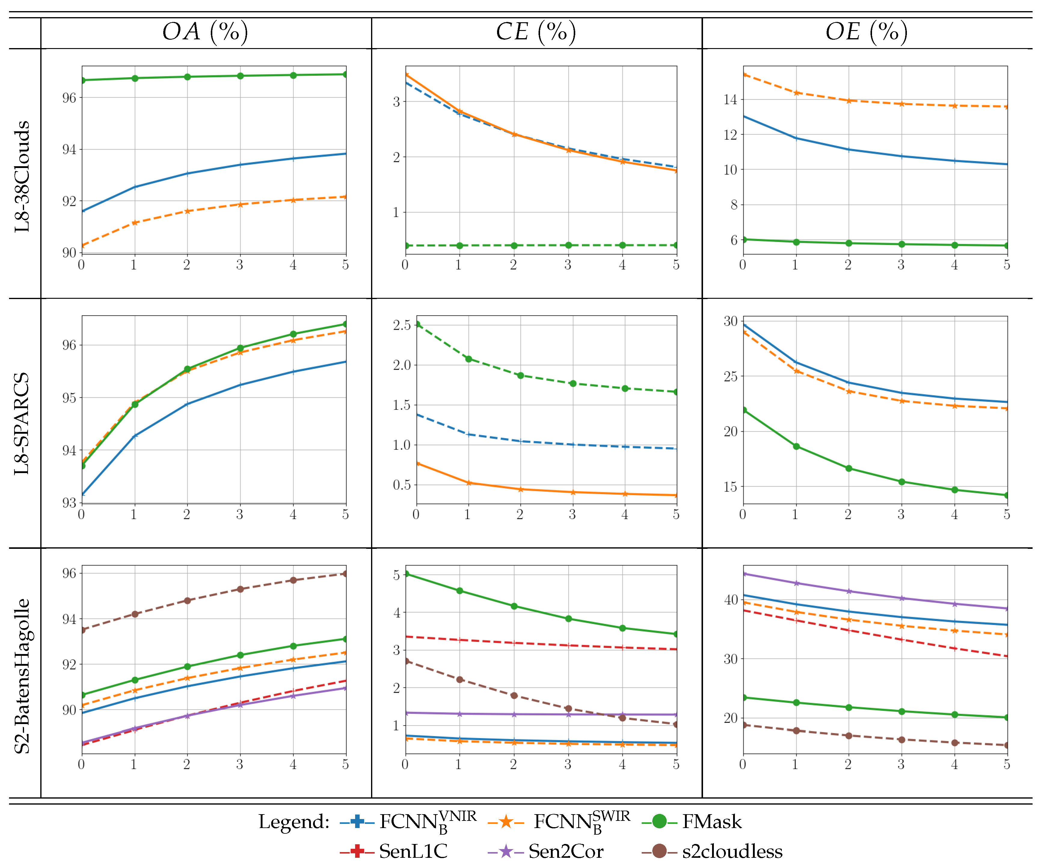
Figure 7 shows the impact of the cloud borders, in terms of OA, CE, and OE, for different increasing exclusion widths. Attending to the L8-38Clouds dataset results, several conclusions can be drawn. On the one hand, models based on are more affected by cloud borders, and both omission and commission errors significantly decrease as the exclusion region is wider. On the contrary, FMask shows a significantly higher performance and a substantially stable behavior for the all w values and metrics for this dataset. This behavior can be explained by the fact that the L8-38Clouds dataset ground truth is not independent of the FMask algorithm since it was used as starting point for the ground truth generation. Consequently, cloud borders of the ground truth and FMask maximally agree.
Conversely, results on the L8-SPARCS and S2-BaetensHagolle datasets show the expected behavior for all the methods: as more difficult pixels around the cloud borders are excluded, the cloud detection accuracy is higher, and the commission and omission errors are lower. These results suggest that none of the analyzed methods present a clear bias for or dependence on these two particular datasets.
The key message to take away is that the ground truth has to be both accurate and representative, but in addition, the proposed algorithms should be evaluated on an independently generated ground truth. The analysis of the performance over the cloud borders, and its eventual deviation from the standard behavior, is a sensible way to measure this dependence between a particular model and the dataset used for evaluation.
6. Discussion and Conclusions
This paper presents cloud detection models based on recent deep learning developments. In particular, we choose fully convolutional neural networks, which excel at exploiting spectral and spatial information in image classification problems when enough training data are available to learn the model parameters. In this context, the objective of our work is two-fold. On the one hand, we want to explore the possibilities to transfer models from one satellite sensor to another. This would mitigate the training data requirements when labeled data are not accessible for a given sensor. Therefore, our aim is to provide an accurate cloud detection model directly learned from real Landsat data that could be also applied to Sentinel-2 images. In order to do that, we take advantage of publicly available and well-known datasets of Landsat images manually annotated for cloud detection studies. On the other hand, we want to benchmark the proposed method against the operational cloud detection algorithms of both Landsat-8 and Sentinel-2. However, we focus not only on the detection accuracy metrics, but also on the analysis of the performance depending on the labeled datasets used for validation. A comprehensive inter-dataset evaluation is carried out by testing each model on several datasets with different characteristics. This provides a realistic view to identify the strengths and weaknesses of the benchmarked models. Moreover, with the aim of contributing to future cloud detection research developments, the code of the proposed cloud detection algorithm for both Landsat-8 and Sentinel-2 images is open source and available in a public repository.
Our experimental results show a very competitive performance of the proposed model when compared to state-of-the-art cloud detection algorithms for Landsat-8. This performance is even better in the case of Sentinel-2, taking into account the fact that no Sentinel-2 data were used to train the models, which emphasizes the effectiveness of the transfer learning strategy from Landsat-8 to Sentinel-2. Although the obtained results did not outperform the custom models designed specifically for Sentinel-2, the proposed transfer learning approach offers competitive results that do not overfit over different datasets. Therefore, it opens the door to the remote sensing community to build general cloud detection models instead of developing tailored models for each single sensor from scratch.
Although the retrieved accuracy values were reasonably good for all the experiments, a high variability was found in the results depending on the dataset used to train or to evaluate the models. All datasets employed in this work are well-established references in the community, but our results reveal that the assumptions and choices made when developing each manual ground truth have an effect and produce certain biases. These biases lead to differences in the performance of a given model across the datasets. Focusing on critical cloud problems such as thin clouds and cloud borders helps to identify models that deviate from the expected behavior in a particular dataset. This behavior can be associated with eventual underlying relationships between the models themselves and the cloud masks used as the ground truth. Therefore, these inter-dataset differences cannot be neglected and should be taken into account when comparing the performances of different methods from different studies.
Author Contributions
D.L.-P.: methodology, software, validation, data curation, and writing; G.M.-G.: conceptualization, methodology, software, and writing; L.G.-C.: conceptualization, methodology, writing, and project administration. All authors read and agreed to the published version of the manuscript.
Funding
This work was supported by the Spanish Ministry of Science and Innovation (projects TEC2016-77741-R and PID2019-109026RB-I00, ERDF) and the European Social Fund.
Institutional Review Board Statement
Not applicable.
Informed Consent Statement
Not applicable.
Data Availability Statement
The data used in this work belong to open-source datasets available in their corresponding references within this manuscript. The code of the pre-trained network architectures and their evaluation on the data can be accessed at https://github.com/IPL-UV/DL-L8S2-UV (accessed on 3 February 2021).
Acknowledgments
We thank the NASA-ESA Cloud Masking Inter-comparison eXercise (CMIX) participants.
Conflicts of Interest
The authors declare no conflict of interest.
References
- Wolanin, A.; Mateo-García, G.; Camps-Valls, G.; Gómez-Chova, L.; Meroni, M.; Duveiller, G.; Liangzhi, Y.; Guanter, L. Estimating and understanding crop yields with explainable deep learning in the Indian Wheat Belt. Environ. Res. Lett. 2020, 15, 1–12. [Google Scholar] [CrossRef]
- Camps-Valls, G.; Gómez-Chova, L.; Muñoz-Marí, J.; Vila-Francés, J.; Amorós-López, J.; Calpe-Maravilla, J. Retrieval of oceanic chlorophyll concentration with relevance vector machines. Remote Sens. Environ. 2006, 105, 23–33. [Google Scholar] [CrossRef]
- Mateo-Garcia, G.; Oprea, S.; Smith, L.; Veitch-Michaelis, J.; Schumann, G.; Gal, Y.; Baydin, A.G.; Backes, D. Flood Detection On Low Cost Orbital Hardware. In Proceedings of the Artificial Intelligence for Humanitarian Assistance and Disaster Response Workshop, 33rd Conference on Neural Information Processing Systems (NeurIPS 2019), Vancouver, BC, Canada, 8–14 December 2019. [Google Scholar]
- Gómez-Chova, L.; Fernández-Prieto, D.; Calpe, J.; Soria, E.; Vila-Francés, J.; Camps-Valls, G. Urban Monitoring using Multitemporal SAR and Multispectral Data. Pattern Recognit. Lett. 2006, 27, 234–243. [Google Scholar] [CrossRef]
- Gómez-Chova, L.; Camps-Valls, G.; Calpe, J.; Guanter, L.; Moreno, J. Cloud-Screening Algorithm for ENVISAT/MERIS Multispectral Images. IEEE Trans. Geosci. Remote Sens. 2007, 45, 4105–4118. [Google Scholar] [CrossRef]
- Zhu, Z.; Wang, S.; Woodcock, C.E. Improvement and expansion of the Fmask algorithm: Cloud, cloud shadow, and snow detection for Landsats 4–7, 8, and Sentinel 2 images. Remote Sens. Environ. 2015, 159, 269–277. [Google Scholar] [CrossRef]
- Louis, J.; Debaecker, V.; Pflug, B.; Main-Knorn, M.; Bieniarz, J.; Mueller-Wilm, U.; Cadau, E.; Gascon, F. Sentinel-2 sen2cor: L2a processor for users. In Proceedings of the Living Planet Symposium, Prague, Czech Republic, 9–13 May 2016; pp. 9–13. [Google Scholar]
- Li, Z.; Shen, H.; Cheng, Q.; Liu, Y.; You, S.; He, Z. Deep learning based cloud detection for medium and high resolution remote sensing images of different sensors. ISPRS J. Photogramm. Remote Sens. 2019, 150, 197–212. [Google Scholar] [CrossRef] [Green Version]
- Shendryk, Y.; Rist, Y.; Ticehurst, C.; Thorburn, P. Deep learning for multi-modal classification of cloud, shadow and land cover scenes in PlanetScope and Sentinel-2 imagery. ISPRS J. Photogramm. Remote Sens. 2019, 157, 124–136. [Google Scholar] [CrossRef]
- Jeppesen, J.H.; Jacobsen, R.H.; Inceoglu, F.; Toftegaard, T.S. A cloud detection algorithm for satellite imagery based on deep learning. Remote Sens. Environ. 2019, 229, 247–259. [Google Scholar] [CrossRef]
- Chai, D.; Newsam, S.; Zhang, H.K.; Qiu, Y.; Huang, J. Cloud and cloud shadow detection in Landsat imagery based on deep convolutional neural networks. Remote Sens. Environ. 2019, 225, 307–316. [Google Scholar] [CrossRef]
- Yang, J.; Guo, J.; Yue, H.; Liu, Z.; Hu, H.; Li, K. CDnet: CNN-Based Cloud Detection for Remote Sensing Imagery. IEEE Trans. Geosci. Remote Sens. 2019, 57, 6195–6211. [Google Scholar] [CrossRef]
- Kanu, S.; Khoja, R.; Lal, S.; Raghavendra, B.; Asha, C. CloudX-net: A robust encoder-decoder architecture for cloud detection from satellite remote sensing images. Remote Sens. Appl. Soc. Environ. 2020, 20, 100417. [Google Scholar] [CrossRef]
- Zhang, J.; Li, X.; Li, L.; Sun, P.; Su, X.; Hu, T.; Chen, F. Lightweight U-Net for cloud detection of visible and thermal infrared remote sensing images. Opt. Quantum Electron. 2020, 52, 397. [Google Scholar] [CrossRef]
- Mateo-García, G.; Laparra, V.; López-Puigdollers, D.; Gómez-Chova, L. Transferring deep learning models for cloud detection between Landsat-8 and Proba-V. ISPRS J. Photogramm. Remote Sens. 2020, 160, 1–17. [Google Scholar] [CrossRef]
- Doxani, G.; Vermote, E.; Roger, J.C.; Gascon, F.; Adriaensen, S.; Frantz, D.; Hagolle, O.; Hollstein, A.; Kirches, G.; Li, F.; et al. Atmospheric Correction Inter-Comparison Exercise. Remote Sens. 2018, 10, 352. [Google Scholar] [CrossRef] [PubMed] [Green Version]
- ESA. CEOS-WGCV ACIX II—CMIX: Atmospheric Correction Inter-Comparison Exercise—Cloud Masking Inter-Comparison Exercise. 2019. Available online: https://earth.esa.int/web/sppa/meetings-workshops/hosted-and-co-sponsored-meetings/acix-ii-cmix-2nd-ws (accessed on 28 January 2020).
- Foga, S.; Scaramuzza, P.L.; Guo, S.; Zhu, Z.; Dilley, R.D., Jr.; Beckmann, T.; Schmidt, G.L.; Dwyer, J.L.; Hughes, M.J.; Laue, B. Cloud detection algorithm comparison and validation for operational Landsat data products. Remote Sens. Environ. 2017, 194, 379–390. [Google Scholar] [CrossRef] [Green Version]
- Hughes, M.J.; Hayes, D.J. Automated Detection of Cloud and Cloud Shadow in Single-Date Landsat Imagery Using Neural Networks and Spatial Post-Processing. Remote Sens. 2014, 6, 4907–4926. [Google Scholar] [CrossRef] [Green Version]
- Mohajerani, S.; Saeedi, P. Cloud-Net: An end-to-end cloud detection algorithm for Landsat 8 imagery. In Proceedings of the IGARSS 2019-2019 IEEE International Geoscience and Remote Sensing Symposium, Yokohama, Japan, 28 July–2 August 2019; pp. 1029–1032. [Google Scholar]
- Hollstein, A.; Segl, K.; Guanter, L.; Brell, M.; Enesco, M. Ready-to-use methods for the detection of clouds, cirrus, snow, shadow, water and clear sky pixels in Sentinel-2 MSI images. Remote Sens. 2016, 8, 666. [Google Scholar] [CrossRef] [Green Version]
- Baetens, L.; Olivier, H. Sentinel-2 Reference Cloud Masks Generated by an Active Learning Method. Available online: https://zenodo.org/record/1460961 (accessed on 19 February 2019).
- Tarrio, K.; Tang, X.; Masek, J.G.; Claverie, M.; Ju, J.; Qiu, S.; Zhu, Z.; Woodcock, C.E. Comparison of cloud detection algorithms for Sentinel-2 imagery. Sci. Remote Sens. 2020, 2, 100010. [Google Scholar] [CrossRef]
- Zekoll, V.; Main-Knorn, M.; Louis, J.; Frantz, D.; Richter, R.; Pflug, B. Comparison of Masking Algorithms for Sentinel-2 Imagery. Remote Sens. 2021, 13, 137. [Google Scholar] [CrossRef]
- Zhu, Z.; Woodcock, C.E. Object-based cloud and cloud shadow detection in Landsat imagery. Remote Sens. Environ. 2012, 118, 83–94. [Google Scholar] [CrossRef]
- Frantz, D.; Haß, E.; Uhl, A.; Stoffels, J.; Hill, J. Improvement of the Fmask algorithm for Sentinel-2 images: Separating clouds from bright surfaces based on parallax effects. Remote Sens. Environ. 2018, 215, 471–481. [Google Scholar] [CrossRef]
- Qiu, S.; Zhu, Z.; He, B. Fmask 4.0: Improved cloud and cloud shadow detection in Landsats 4–8 and Sentinel-2 imagery. Remote Sens. Environ. 2019, 231, 111205. [Google Scholar] [CrossRef]
- Sentinel Hub Team. Sentinel Hub’s Cloud Detector for Sentinel-2 Imagery. 2017. Available online: https://github.com/sentinel-hub/sentinel2-cloud-detector (accessed on 28 January 2020).
- Friedman, J.H. Greedy function approximation: A gradient boosting machine. Ann. Statist. 2001, 29, 1189–1232. [Google Scholar] [CrossRef]
- Ke, G.; Meng, Q.; Finley, T.; Wang, T.; Chen, W.; Ma, W.; Ye, Q.; Liu, T.Y. LightGBM: A Highly Efficient Gradient Boosting Decision Tree. In Advances in Neural Information Processing Systems 30; Guyon, I., Luxburg, U.V., Bengio, S., Wallach, H., Fergus, R., Vishwanathan, S., Garnett, R., Eds.; Curran Associates, Inc.: Dutchess County, NY, USA, 2017; pp. 3146–3154. [Google Scholar]
- Hagolle, O.; Huc, M.; Pascual, D.V.; Dedieu, G. A multi-temporal method for cloud detection, applied to FORMOSAT-2, VENuS, LANDSAT and SENTINEL-2 images. Remote Sens. Environ. 2010, 114, 1747–1755. [Google Scholar] [CrossRef] [Green Version]
- Hollstein, A.; Segl, K.; Guanter, L.; Brell, M.; Enesco, M. Database File of Manually Classified Sentinel-2A Data. 2017. Available online: https://gitext.gfz-potsdam.de/EnMAP/sentinel2_manual_classification_clouds/blob/master/20170710_s2_manual_classification_data.h5 (accessed on 28 January 2020).
- U.S. Geological Survey. L8 Biome Cloud Validation Masks; U.S. Geological Survey Data Release; U.S. Geological Survey: Reston, VA, USA, 2016. [Google Scholar] [CrossRef]
- U.S. Geological Survey. L8 SPARCS Cloud Validation Masks; U.S. Geological Survey Data Release; U.S. Geological Survey: Reston, VA, USA, 2016. [Google Scholar] [CrossRef]
- Mohajerani, S.; Krammer, T.A.; Saeedi, P. A Cloud Detection Algorithm for Remote Sensing Images Using Fully Convolutional Neural Networks. In Proceedings of the 2018 IEEE 20th International Workshop on Multimedia Signal Processing (MMSP), Vancouver, BC, Canada, 29–31 August 2018; pp. 1–5. [Google Scholar] [CrossRef] [Green Version]
- Baetens, L.; Desjardins, C.; Hagolle, O. Validation of Copernicus Sentinel-2 Cloud Masks Obtained from MAJA, Sen2Cor, and FMask Processors Using Reference Cloud Masks Generated with a Supervised Active Learning Procedure. Remote Sens. 2019, 11, 433. [Google Scholar] [CrossRef] [Green Version]
- Long, J.; Shelhamer, E.; Darrell, T. Fully convolutional networks for semantic segmentation. In Proceedings of the 2015 IEEE Conference on Computer Vision and Pattern Recognition (CVPR), Boston, MA, USA, 7–12 June 2015; pp. 3431–3440. [Google Scholar] [CrossRef] [Green Version]
- Zeiler, M.D.; Krishnan, D.; Taylor, G.W.; Fergus, R. Deconvolutional networks. In Proceedings of the 2010 IEEE Computer Society Conference on Computer Vision and Pattern Recognition, San Francisco, CA, USA, 13–18 June 2010. [Google Scholar]
- Ronneberger, O.; Fischer, P.; Brox, T. U-Net: Convolutional Networks for Biomedical Image Segmentation. In Medical Image Computing and Computer-Assisted Intervention–MICCAI 2015; Springer: Cham, Switzerland, 2015; pp. 234–241. [Google Scholar] [CrossRef] [Green Version]
- Wieland, M.; Li, Y.; Martinis, S. Multi-sensor cloud and cloud shadow segmentation with a convolutional neural network. Remote Sens. Environ. 2019, 230, 111203. [Google Scholar] [CrossRef]
- Hughes, M.J.; Kennedy, R. High-Quality Cloud Masking of Landsat 8 Imagery Using Convolutional Neural Networks. Remote Sens. 2019, 11, 2591. [Google Scholar] [CrossRef] [Green Version]
- Badrinarayanan, V.; Kendall, A.; Cipolla, R. Segnet: A deep convolutional encoder-decoder architecture for image segmentation. IEEE Trans. Pattern Anal. Mach. Intell. 2017, 39, 2481–2495. [Google Scholar] [CrossRef] [PubMed]
- Irish, R.R.; Barker, J.L.; Goward, S.N.; Arvidson, T. Characterization of the Landsat-7 ETM+ Automated Cloud-Cover Assessment (ACCA) Algorithm. Photogramm. Eng. Remote Sens. 2006, 72, 1179–1188. [Google Scholar] [CrossRef]
- Raiyani, K.; Gonçalves, T.; Rato, L.; Salgueiro, P.; Marques da Silva, J.R. Sentinel-2 Image Scene Classification: A Comparison between Sen2Cor and a Machine Learning Approach. Remote Sens. 2021, 13, 300. [Google Scholar] [CrossRef]
- Ploton, P.; Mortier, F.; Réjou-Méchain, M.; Barbier, N.; Picard, N.; Rossi, V.; Dormann, C.; Cornu, G.; Viennois, G.; Bayol, N.; et al. Spatial validation reveals poor predictive performance of large-scale ecological mapping models. Nat. Commun. 2020, 11, 1–11. [Google Scholar] [CrossRef] [PubMed]
- Mateo-García, G.; Laparra, V.; López-Puigdollers, D.; Gómez-Chova, L. Cross-Sensor Adversarial Domain Adaptation of Landsat-8 and Proba-V Images for Cloud Detection. IEEE J. Sel. Top. Appl. Earth Obs. Remote Sens. 2021, 14, 747–761. [Google Scholar] [CrossRef]
- Kingma, D.P.; Ba, J. Adam: A Method for Stochastic Optimization. In Proceedings of the 3rd International Conference on Learning Representations, (ICLR 2015), San Diego, CA, USA, 7–9 May 2015; pp. 1–13. [Google Scholar]
- Abadi, M.; Agarwal, A.; Barham, P.; Brevdo, E.; Chen, Z.; Citro, C.; Corrado, G.S.; Davis, A.; Dean, J.; Devin, M.; et al. TensorFlow: Large-Scale Machine Learning on Heterogeneous Systems. 2015. Available online: tensorflow.org (accessed on 3 February 2021).
- USGS. Comparison of Sentinel-2 and Landsat. 2015. Available online: http://www.usgs.gov/centers/eros/science/usgs-eros-archive-sentinel-2-comparison-sentinel-2-and-landsat (accessed on 28 January 2020).
Figure 1.
Location of the Landsat-8 and Sentinel-2 images in each dataset. Each image includes a manually generated cloud mask to be used as the ground truth. SPARCS, Spatial Procedures for Automated Removal of Cloud and Shadow.
Figure 1.
Location of the Landsat-8 and Sentinel-2 images in each dataset. Each image includes a manually generated cloud mask to be used as the ground truth. SPARCS, Spatial Procedures for Automated Removal of Cloud and Shadow.


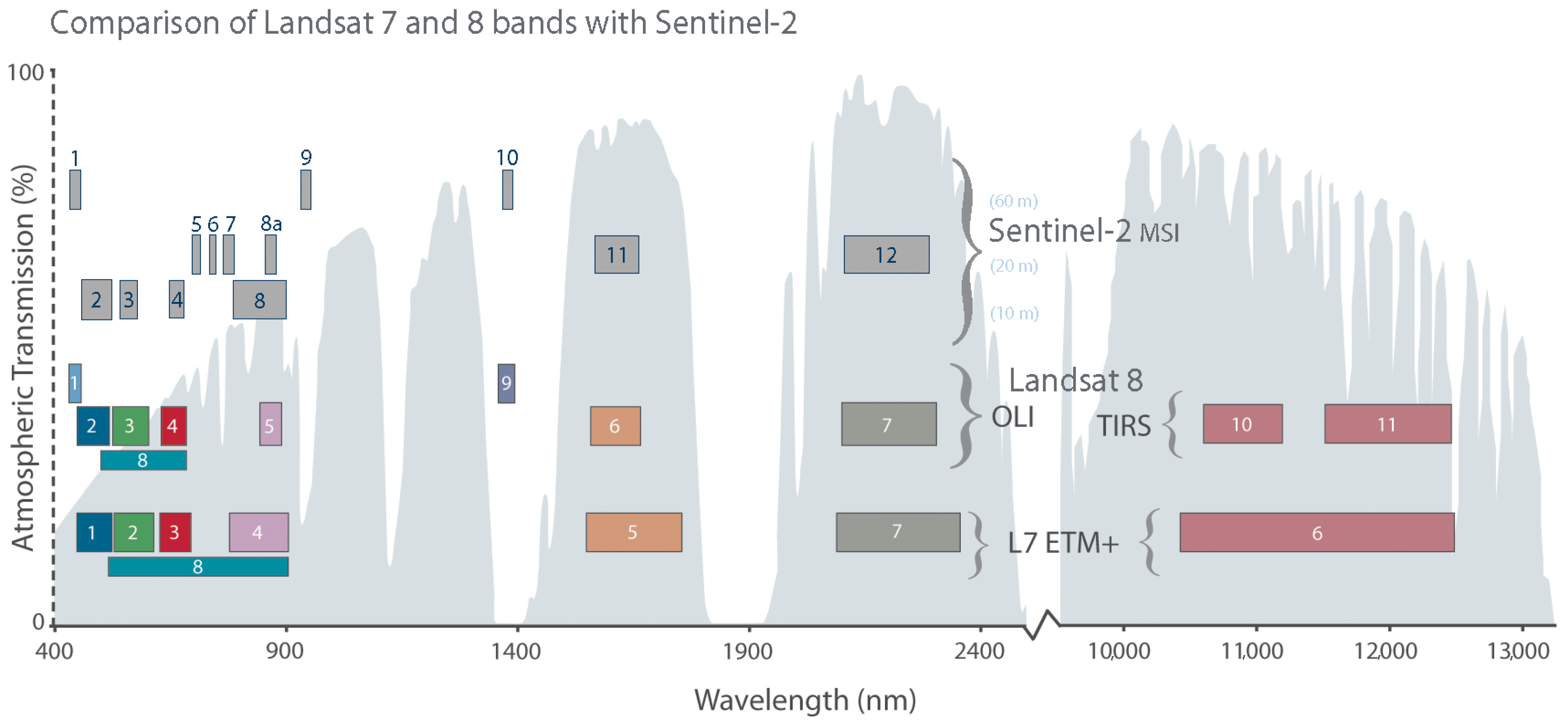
Figure 3.
Comparison of spectral bands between Sentinel-2 and Landsat-8: overlapping response with similar characteristics for the coastal aerosol (440 nm), visible (490–800 nm), and SWIR (1300–2400 nm) spectral bands. Credits: Image from [49].
Figure 3.
Comparison of spectral bands between Sentinel-2 and Landsat-8: overlapping response with similar characteristics for the coastal aerosol (440 nm), visible (490–800 nm), and SWIR (1300–2400 nm) spectral bands. Credits: Image from [49].

Figure 4.
Visual differences between the ground truth and the obtained cloud masks ( and FMask) over three scenes from the L8-SPARCS dataset. Each row displays a different scene, and models are arranged in columns. The first column shows RGB images, and the models are compared from the second to last columns. Differences are shown, composed of three different colors. Surface reflectance is shown for pixels identified as clear in both the ground truth and predicted cloud mask.

Figure 5.
Visual differences between the ground truth and , operational L2A processor Sen2Cor, and FMask for three Sentinel-2 images from the S2-BaetensHagolle dataset. Each row displays a different scene, and the models are arranged by columns. The first column shows RGB. Comparisons between the cloud masks and ground truth are superimposed to the RGB images in the other columns.

Figure 6.
The first column shows the RGB composite, with cloudy pixels highlighted in yellow, for a Sentinel-2 and a Landsat-8 image. The second and third columns show the excluded pixels in green around cloud edges for and , respectively.
Figure 6.
The first column shows the RGB composite, with cloudy pixels highlighted in yellow, for a Sentinel-2 and a Landsat-8 image. The second and third columns show the excluded pixels in green around cloud edges for and , respectively.

Figure 7.
Evaluation of the models comparing performance metrics (y-axis) with respect to the w values (x-axis) in the cloud masks. Each row corresponds to a different evaluation dataset, and each column represents a different performance metric in percentage: overall accuracy, commission error, and omission error, respectively.


Table 1.
Ground truth statistics of each of the Landsat-8 and Sentinel-2 datasets.
| Dataset | Labels | # of Scenes | # of Pixels | Thick Clouds % | Thin Clouds % | Clear % | Invalid % |
|---|---|---|---|---|---|---|---|
| L8-Biome | full-scene | 96 | 4.82 × 10 | 21.15 | 9.37 | 33.19 | 36.28 |
| L8-SPARCS | full-scene | 80 | 0.08 × 10 | 19.37 | NA | 80.63 | 0 |
| L8-38Clouds | full-scene | 38 | 1.74 × 10 | 30.91 | NA | 28.04 | 41.05 |
| S2-Hollstein | pixels | 59 | 3.01 × 10 | 16.18 | 16.61 | 67.21 | 0 |
| S2-BaetensHagolle | full-scene | 35 | 0.41 × 10 | 11.35 | 9.45 | 65.08 | 14.12 |
These datasets do not distinguish between thin and thick clouds.
Table 2.
Summary of the validation schemes used in different works in the literature related to deep learning-based methods applied to cloud detection in Landsat-8 and Sentinel-2 imagery. MSCFF, multi-scale feature extraction and feature fusion.
Table 2.
Summary of the validation schemes used in different works in the literature related to deep learning-based methods applied to cloud detection in Landsat-8 and Sentinel-2 imagery. MSCFF, multi-scale feature extraction and feature fusion.
| Work Reference | Intra-Dataset | Inter-Dataset | Cross-Sensor |
|---|---|---|---|
| RS-Net [10] | ✗ | ✗ | |
| Hughes et al. [41] | ✗ | ||
| SegNet [11] | ✗ | ||
| Cloud-Net [20] | ✗ | ||
| MSCFF [8] | ✗ | ||
| CloudX-net [13] | ✗ | ||
| CDnet [12] | ✗ | ||
| Lightweight U-Net [14] | ✗ | ||
| LeNet [44] | ✗ | ||
| Shendryk et al. [9] | ✗ | ✗ | ✗ |
| Wieland et al. [40] | ✗ | ✗ | ✗ |
| Mateo-Garcia et al. [15] | ✗ | ✗ |
Using an unpublished dataset of 14 1024 × 1024 images.
Table 3.
Results of (with and without SWIR bands), FMask, and MSCFF [8] evaluated on 19 test images from the L8-Biome dataset.
Table 3.
Results of (with and without SWIR bands), FMask, and MSCFF [8] evaluated on 19 test images from the L8-Biome dataset.
| Model | OA% () | CE% () | OE% () |
|---|---|---|---|
| 93.16 (0.41) | 7.78 (1.22) | 5.97 (0.93) | |
| 94.06 (0.30) | 5.68 (0.80) | 6.18 (0.39) | |
| 94.35 (0.34) | 5.36 (0.78) | 5.91 (0.40) | |
| [8] | 93.94 | 6.35 | 5.48 |
| [8] | 94.96 | 4.16 | 6.07 |
| FMask (results from [8]) | 89.59 | 13.38 | 6.99 |
Table 4.
Results of (with and without SWIR bands), RS-Net (VNIR and ALL configurations), and FMask evaluated on the L8-SPARCS dataset.
Table 4.
Results of (with and without SWIR bands), RS-Net (VNIR and ALL configurations), and FMask evaluated on the L8-SPARCS dataset.
| Model | OA% | CE% | OE% |
|---|---|---|---|
| 92.69 (0.45) | 1.99 (0.68) | 29.46 (1.44) | |
| 93.57 (0.17) | 0.85 (0.21) | 29.68 (0.90) | |
| [10] | 92.53 | 0.76 | 35.44 |
| [10] | 93.26 | 2.19 | 27.66 |
| FMask (results from [10]) | 92.47 | 6.03 | 13.79 |
Table 5.
Results of models and FMask evaluated on the L8-38Clouds dataset.
| Model | OA% | CE% | OE% |
|---|---|---|---|
| 91.39 (0.46) | 4.04 (0.73) | 12.76 (1.24) | |
| 90.36 (0.55) | 3.63 (0.48) | 15.08 (1.20) | |
| FMask | 96.66 | 0.39 | 6.01 |
Table 6.
Results of the models, s2cloudless, and FMask evaluated on the S2-BaetensHagolle dataset.
| Thick and Thin Clouds | Thick Clouds Only | |||||
|---|---|---|---|---|---|---|
| OA% | CE% | OE% | OA% | CE% | OE% | |
| 89.79 (0.31) | 0.91 (0.25) | 40.38 (1.77) | 94.99 (0.21) | 0.90 (0.25) | 29.54 (1.81) | |
| 89.81 (0.28) | 0.70 (0.19) | 40.99 (1.34) | 95.16 (0.22) | 0.70 (0.20) | 29.59 (1.77) | |
| s2cloudless | 93.51 | 2.71 | 18.77 | 95.94 | 2.70 | 12.23 |
| Sen2Cor | 88.55 | 1.33 | 44.35 | 93.21 | 1.32 | 41.36 |
| SenL1C | 88.45 | 3.35 | 38.14 | 89.60 | 3.31 | 52.81 |
| FMask | 90.64 | 5.02 | 23.42 | 90.54 | 4.96 | 27.72 |
Results of 33 out of 35 images for the Sen2Cor algorithm.
Table 7.
Results of models, s2cloudless, and FMask evaluated on the pixel-wise S2-Hollstein dataset.
Table 7.
Results of models, s2cloudless, and FMask evaluated on the pixel-wise S2-Hollstein dataset.
| Thick and Thin Clouds | Thick Clouds Only | |||||
|---|---|---|---|---|---|---|
| OA% | CE% | OE% | OA% | CE% | OE% | |
| 87.36 (0.62) | 3.25 (1.36) | 31.90 (1.54) | 96.65 (0.99) | 3.25 (1.36) | 3.77 (1.71) | |
| 87.36 (0.51) | 3.02 (0.86) | 32.35 (0.70) | 97.19 (0.70) | 3.03 (0.86) | 1.87 (0.50) | |
| s2cloudless | 92.80 | 5.39 | 10.91 | 95.20 | 5.39 | 2.37 |
| SenL1C | 84.06 | 19.30 | 9.04 | 83.04 | 19.30 | 7.25 |
| FMask | 86.56 | 16.03 | 8.13 | 86.14 | 16.03 | 4.84 |
Publisher’s Note: MDPI stays neutral with regard to jurisdictional claims in published maps and institutional affiliations. |
© 2021 by the authors. Licensee MDPI, Basel, Switzerland. This article is an open access article distributed under the terms and conditions of the Creative Commons Attribution (CC BY) license (http://creativecommons.org/licenses/by/4.0/).
Share and Cite
MDPI and ACS Style
López-Puigdollers, D.; Mateo-García, G.; Gómez-Chova, L. Benchmarking Deep Learning Models for Cloud Detection in Landsat-8 and Sentinel-2 Images. Remote Sens. 2021, 13, 992. https://0-doi-org.brum.beds.ac.uk/10.3390/rs13050992
AMA Style
López-Puigdollers D, Mateo-García G, Gómez-Chova L. Benchmarking Deep Learning Models for Cloud Detection in Landsat-8 and Sentinel-2 Images. Remote Sensing. 2021; 13(5):992. https://0-doi-org.brum.beds.ac.uk/10.3390/rs13050992
Chicago/Turabian StyleLópez-Puigdollers, Dan, Gonzalo Mateo-García, and Luis Gómez-Chova. 2021. "Benchmarking Deep Learning Models for Cloud Detection in Landsat-8 and Sentinel-2 Images" Remote Sensing 13, no. 5: 992. https://0-doi-org.brum.beds.ac.uk/10.3390/rs13050992
Note that from the first issue of 2016, this journal uses article numbers instead of page numbers. See further details here.