Author Contributions
Conceptualization, B.C. and C.L.; methodology, C.L. and B.X.; validation, C.L., B.X. and C.H.; formal analysis, B.C., B.X. and C.L.; investigation, C.L., X.L. and C.H.; resources, B.C.; data curation, C.L., X.L., N.J., C.H. and J.C.; writing—original draft preparation, C.L.; writing—review and editing, B.C. and B.X.; visualization, C.L. and C.H.; supervision, B.C. and B.X.; project administration, B.C.; funding acquisition, B.C. All authors read and agreed to the published version of the manuscript.
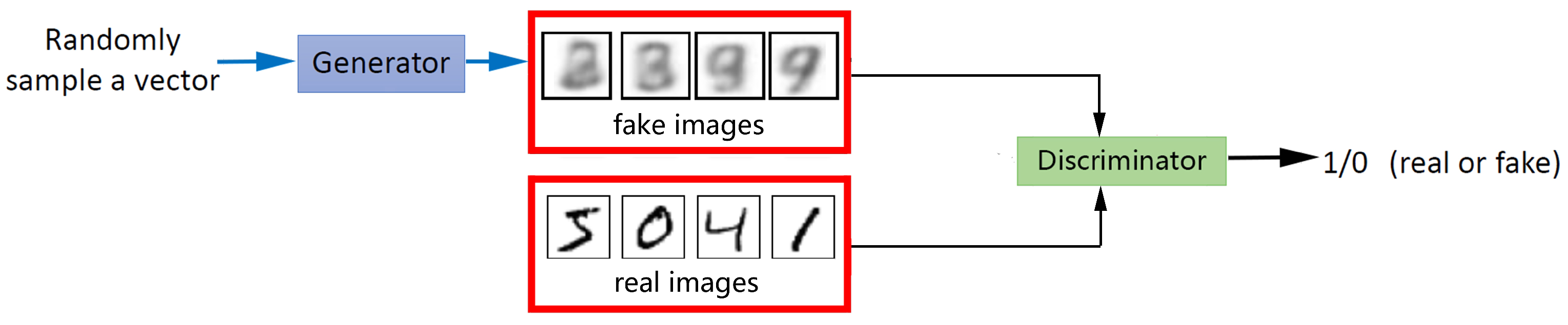
Figure 1.
GAN architecture.
Figure 1.
GAN architecture.
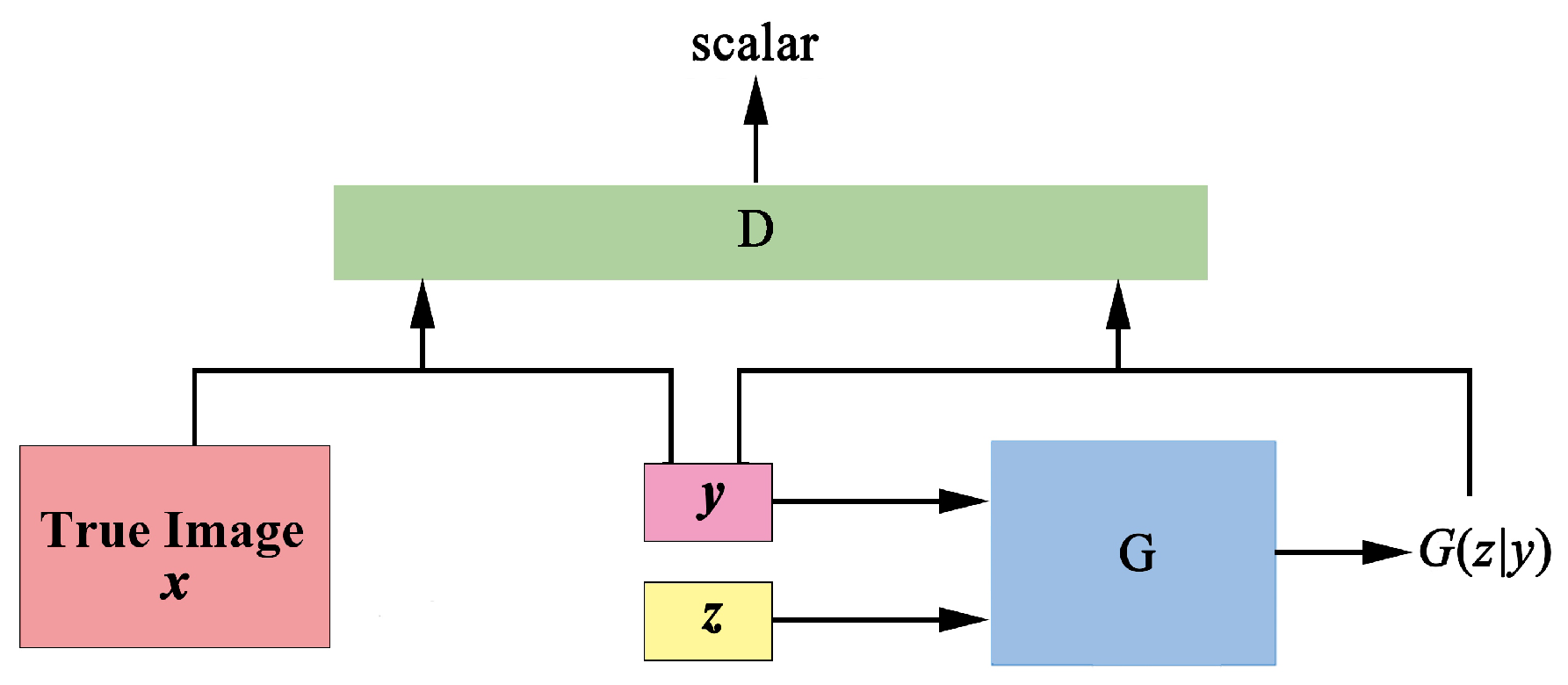
Figure 2.
Conditional generative adversarial net (CGAN) architecture.
Figure 2.
Conditional generative adversarial net (CGAN) architecture.
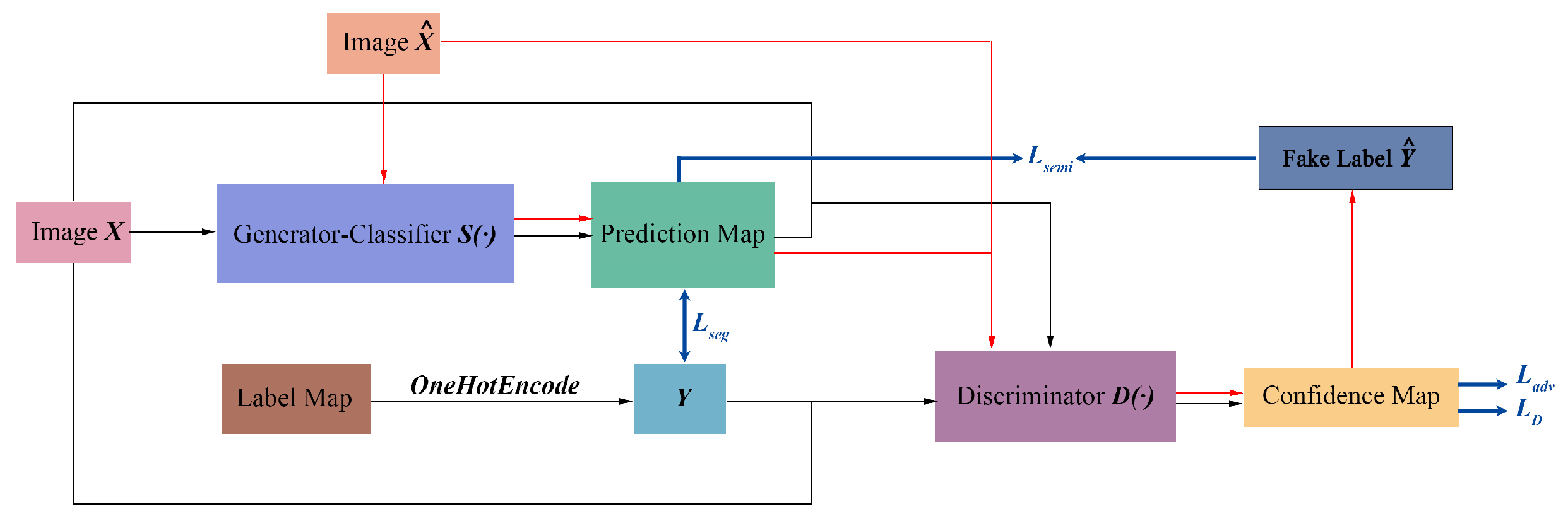
Figure 3.
Semi-/weakly-supervised semantic segmentation network (Semi-SSN) architecture. The black workflow is the process of training labeled image X; The red workflow is the process of training unlabeled image .
Figure 3.
Semi-/weakly-supervised semantic segmentation network (Semi-SSN) architecture. The black workflow is the process of training labeled image X; The red workflow is the process of training unlabeled image .
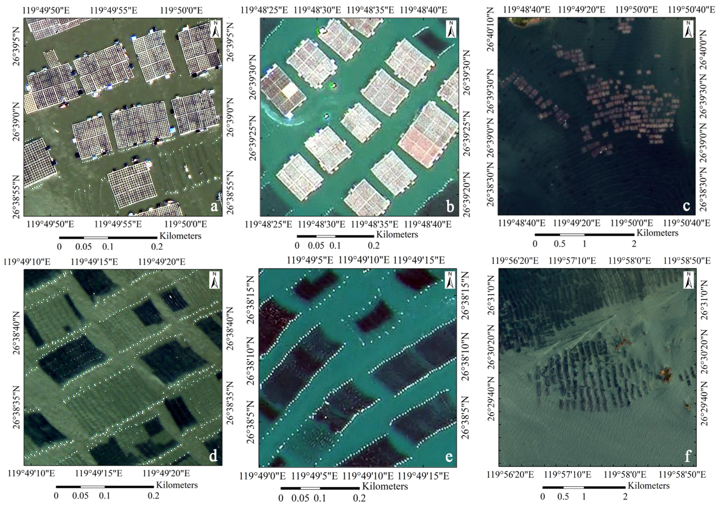
Figure 4.
Two main types of aquaculture areas. (a) Cage culture area in a GF-2 image; (b) cage culture area in a GF-1(PMS) image; (c) cage culture area in a GF-1(WFV) image; (d) raft culture area in a GF-2 image; (e) raft culture area in a GF-1(PMS) image; (f) raft culture area in a GF-1(WFV) image.
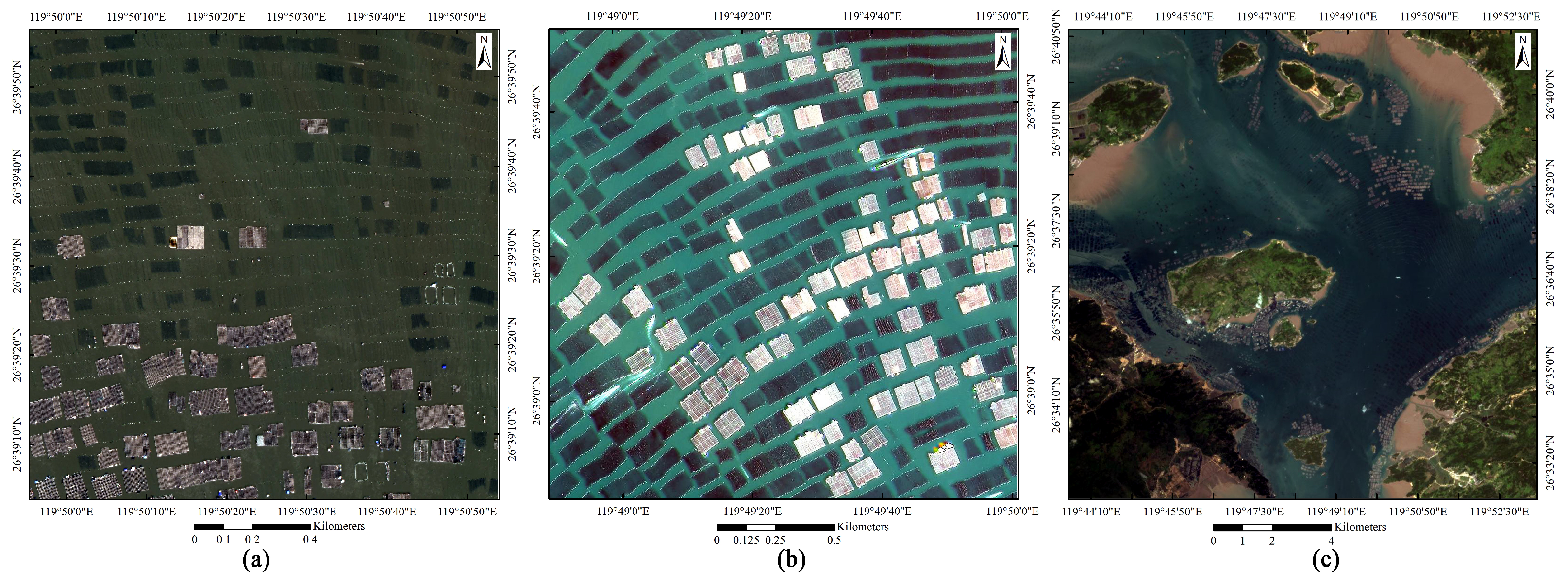
Figure 5.
Test image. (a) GF-2 test image; (b) GF-1 (PMS) test image; (c) GF-1 (WFV) test image.
Figure 5.
Test image. (a) GF-2 test image; (b) GF-1 (PMS) test image; (c) GF-1 (WFV) test image.
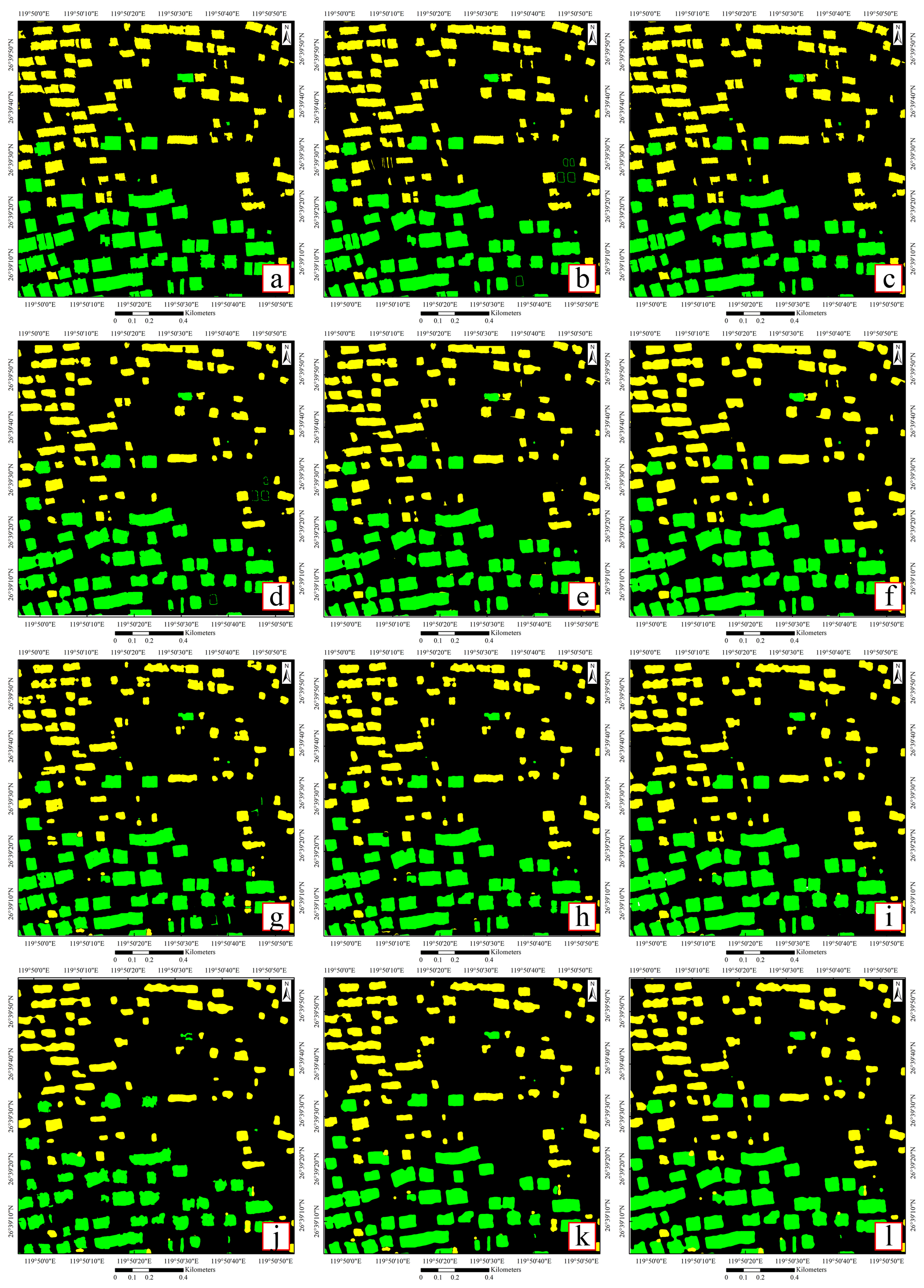
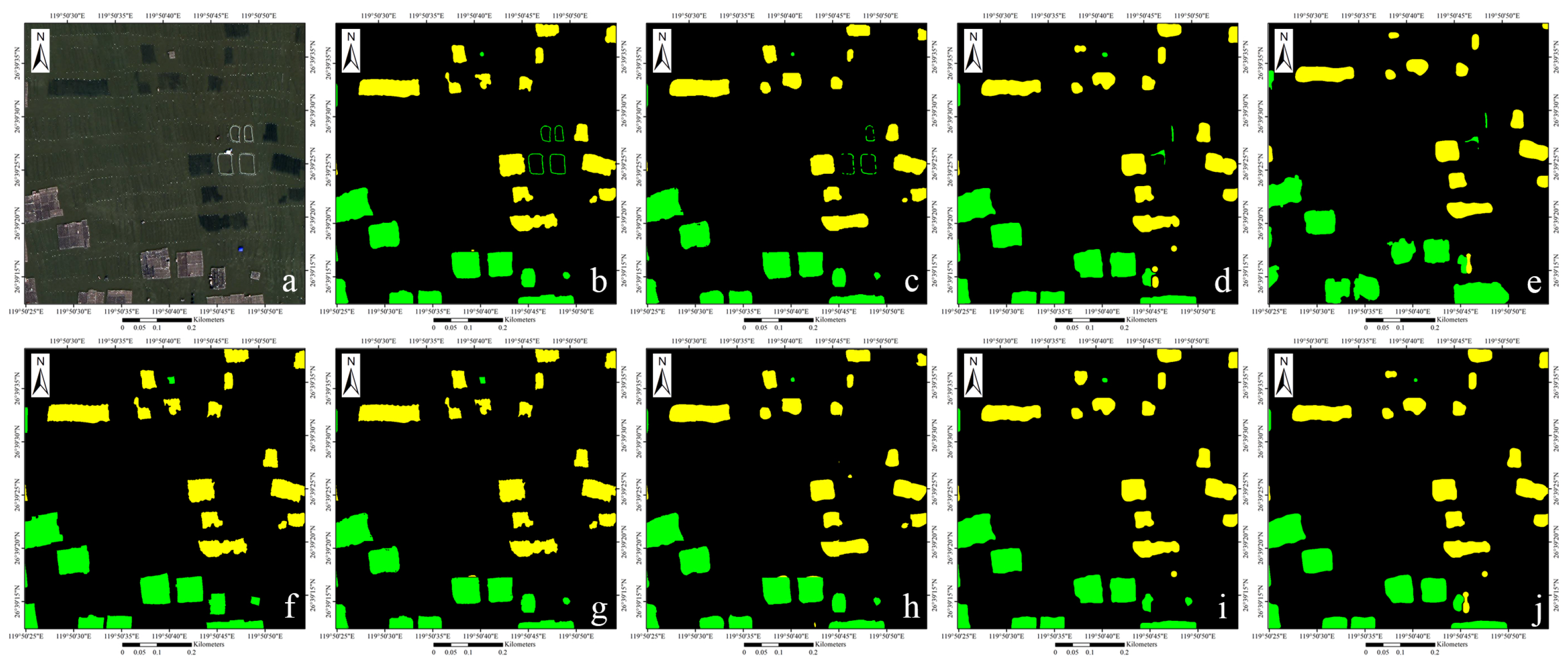
Figure 6.
Extraction result, where green stands for cage culture areas, yellow stands for raft culture areas, and black for background. (a) Ground truth; (b) labeled data amount: full, model: baseline; (c) labeled data amount: full, model: baseline + ; (d) labeled data amount: 1/2, model: baseline; (e) labeled data amount: 1/2, model: baseline + ; (f) labeled data amount: 1/2, model: baseline + + ; (g) labeled data amount: 1/4, model: baseline; (h) labeled data amount: 1/4, model: baseline + ; (i) labeled data amount: 1/4, model: baseline + + ; (j) labeled data amount: 1/8, model: baseline; (k) Labeled data amount: 1/8, model: baseline + ; (l) labeled data amount: 1/8, model: baseline + + .
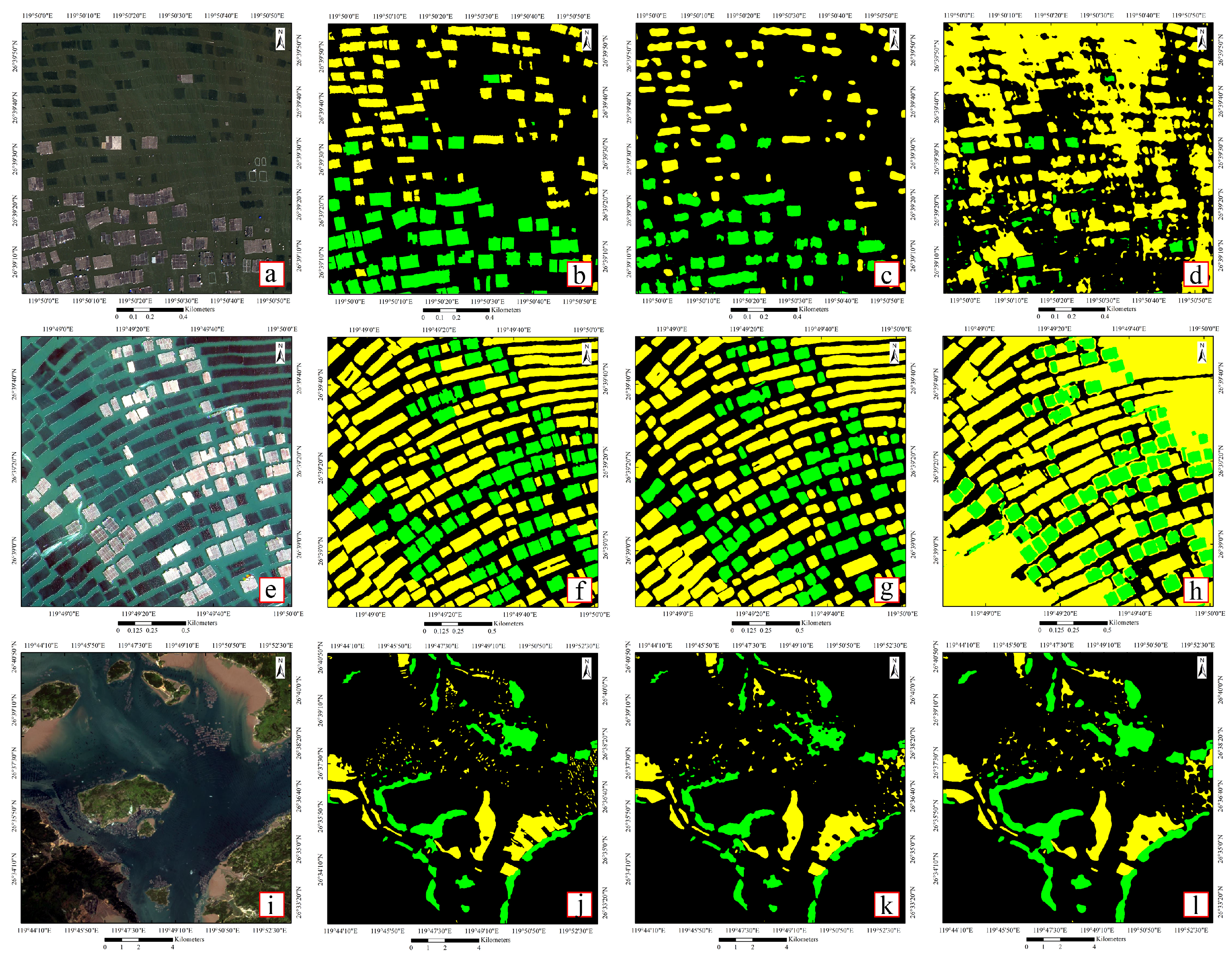
Figure 7.
Extraction result based on the weakly-supervised method. (a) GF-2 Image; (b) ground truth of GF-2 image; (c) extraction result of GF-2 image based on labeled GF-1 (PMS) data; (d) extraction result of GF-2 image based on labeled GF-1 (WFV) data; (e) GF-1 (PMS) image; (f) ground truth of GF-1 (PMS) image; (g) extraction result of GF-1 (PMS) image based on labeled GF-2 data; (h) extraction result of GF-1 (PMS) image based on labeled GF-1 (WFV) data; (i) GF-1 (WFV) image; (j) ground truth of GF-1 (WFV) image; (k) extraction result of GF-1 (WFV) image based on labeled GF-2 data; (l) extraction result of GF-1 (WFV) image based on labeled GF-1 (PMS) data.
Figure 8.
The details of the extraction result. (a) image; (b) labeled data amount: full, model: baseline; (c) labeled data amount: 1/2, model: baseline; (d) labeled data amount: 1/4, model: baseline; (e) labeled data amount: 1/8, model: baseline; (f) ground truth; (g) labeled data amount: full, model: baseline + ; (h) labeled data amount: 1/2, model: baseline + ; (i) labeled data amount: 1/4, model: baseline + ; (j) labeled data amount: 1/8, model: baseline + .
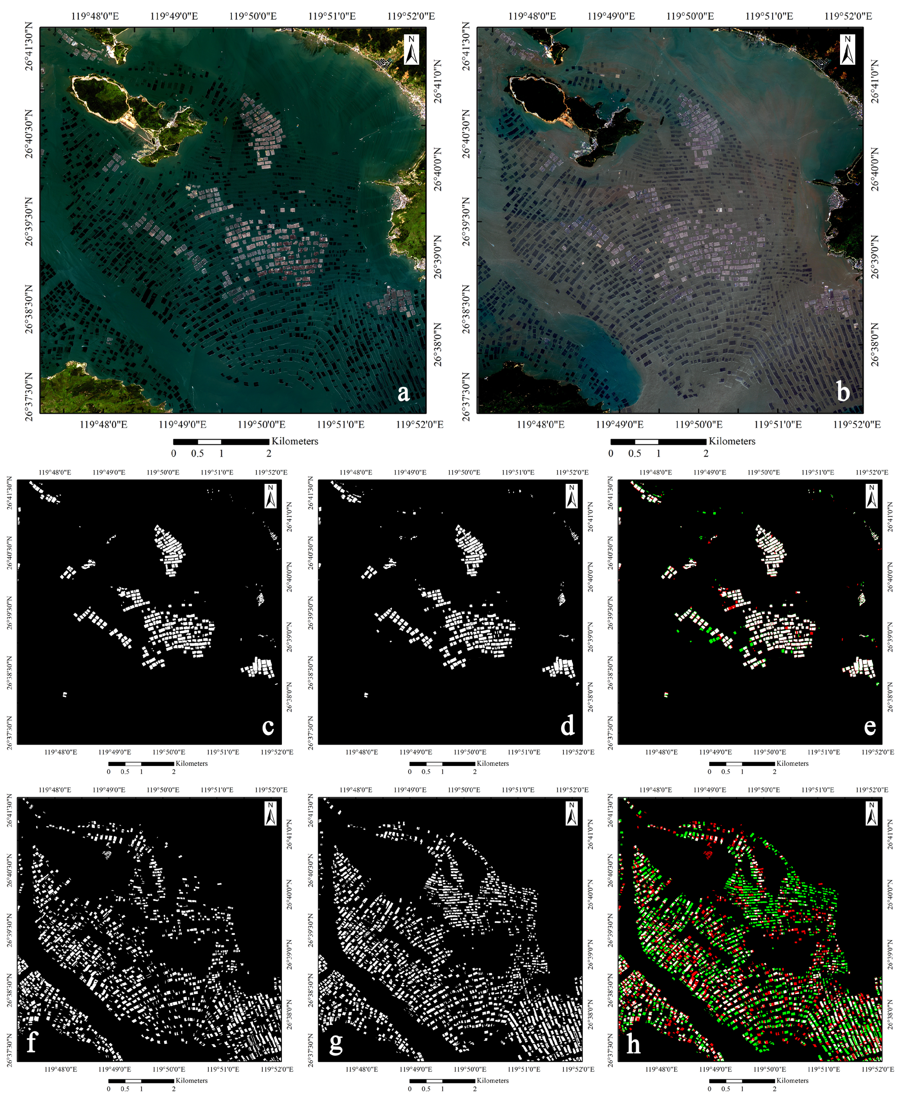
Figure 9.
Change detection before and after typhoon “Maria”, where white stands for coastal aquaculture areas, red stands for the reduction of aquaculture areas, and green stands for the increase of aquaculture areas. (a) GF-1 (PMS) image imaged on 8 April 2018; (b) GF-1 (PMS) image imaged on 19 September 2018; (c) cage culture area before typhoon “Maria”; (d) cage culture area after typhoon “Maria”; (e) change area of the cage culture area; (f) raft culture area before typhoon “Maria”; (g) raft culture area after typhoon “Maria”; (h) change area of the raft culture area.
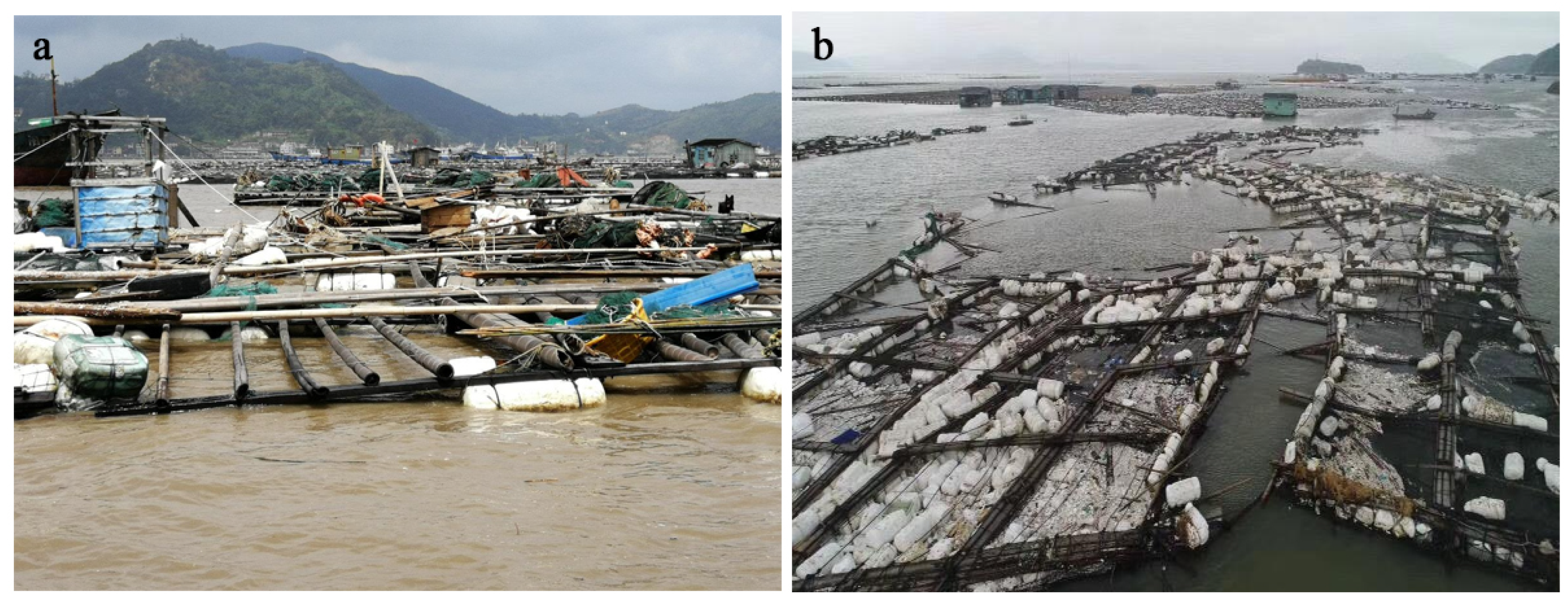
Figure 10.
Field investigation of disaster situation. (a) Cage culture area; (b) raft culture area.
Figure 10.
Field investigation of disaster situation. (a) Cage culture area; (b) raft culture area.
Figure 11.
Production monitoring, where white stands for coastal aquaculture areas, red stands for the reduction of aquaculture areas, and green stands for the increase of aquaculture areas. (a) GF-2 image imaged on 22 June 2016; (b) GF-2 image imaged on 19 September 2016; (c) cage culture area on 22 June 2016; (d) cage culture area on 19 September 2016; (e) change area of the cage culture area; (f) Raft culture area on June 22, 2016; (g) raft culture area on 19 September 2016; (h) change area of the raft culture area.
Figure 12.
The distribution map of the coastal aquaculture areas.
Figure 12.
The distribution map of the coastal aquaculture areas.
Table 1.
Context network. In this network, C is the category number.
Table 1.
Context network. In this network, C is the category number.
| Layer | 1 | 2 | 3 | 4 | 5 | 6 | 7 | 8 |
|---|
| Dilated rate | 1 | 1 | 2 | 4 | 8 | 16 | 1 | 1 |
| Kernel size | 3 × 3 | 3 × 3 | 3 × 3 | 3 × 3 | 3 × 3 | 3 × 3 | 3 × 3 | 1 × 1 |
| Filter | 2C | 2C | 4C | 8C | 16C | 32C | 32C | C |
Table 2.
Data sources and their uses.
Table 2.
Data sources and their uses.
| Data Source | Use | Date | Central Geographical Coordinates |
|---|
| GF-2 | Sample Construction | 30 March 2019 | 119°52 E 26°43 N |
| 30 March 2019 | 119°49 E 26°32 N |
| Production Monitoring | 22 June 2016 | 119°54 E 26°42 N |
| 19 September 2016 | 119°48 E 26°42 N |
| GF-1(PMS) | Sample Construction | 23 September 2019 | 119°56 E 26°49 N |
| Disaster Emergency Response | 8 April 2018 | 119°42 E 26°36 N |
| 19 September 2018 | 119°54 E 26°36 N |
| GF-1(WFV) | Sample Construction | 28 January 2019 | 119°50 E 26°55 N |
| Map making | 15 May 2016 | 119°55 E 26°54 N |
| 15 July 2016 | 119°50 E 26°50 N |
Table 3.
The technical indicators of the GF-2, GF-1(PMS), and GF-1(WFV) images.
Table 3.
The technical indicators of the GF-2, GF-1(PMS), and GF-1(WFV) images.
| Spectral Range | Resolution |
|---|
| GF-2 | GF-1(PMS) | GF-1(WFV) |
|---|
| Pan | 0.45–0.90 m | 1 m | 2 m | 16 m |
| Multispectral | 0.45–0.52 m | 4 m | 8 m | 16 m |
| 0.52–0.59 m | 4 m | 8 m | 16 m |
| 0.63–0.69 m | 4 m | 8 m | 16 m |
| 0.77–0.89 m | 4 m | 8 m | 16 m |
Table 4.
Division of samples in the semi-supervised experiment.
Table 4.
Division of samples in the semi-supervised experiment.
| Labeled Data Amount | Training Set | Validation Set |
|---|
| Labeled | Unlabeled |
|---|
| Full | 8000 | - | 2000 |
| 1/2 | 4000 | 4000 | 2000 |
| 1/4 | 2000 | 6000 | 2000 |
| 1/8 | 1000 | 7000 | 2000 |
Table 5.
Division of samples in the weakly-supervised experiment.
Table 5.
Division of samples in the weakly-supervised experiment.
| Labeled Data/Unlabeled Data | Training Set | Validation Set |
|---|
| Labeled | Unlabeled |
|---|
| GF-2/GF-1(PMS) | 1000 | 7000 | 2000 |
| GF-2/GF-1(WFV) | 1000 | 7000 | 2000 |
| GF-1(PMS)/GF-2 | 1000 | 7000 | 2000 |
| GF-1(PMS)/GF-1(WFV) | 1000 | 7000 | 2000 |
| GF-1(WFV)/GF-2 | 1000 | 7000 | 2000 |
| GF-1(WFV)/GF-1(PMS) | 1000 | 7000 | 2000 |
Table 6.
on the validation set and test set.
Table 6.
on the validation set and test set.
| | Methods | Labeled Data Amount |
|---|
| 1/8 | 1/4 | 1/2 | Full |
|---|
| Validation Accuracy | baseline | 0.7047 | 0.7434 | 0.7937 | 0.8530 |
| baseline + | 0.7512 | 0.7842 | 0.8253 | 0.8725 |
| baseline + + | 0.7961 | 0.8103 | 0.8417 | N/A |
| Test Accuracy | baseline | 0.6842 | 0.7618 | 0.8036 | 0.8847 |
| baseline + | 0.7635 | 0.7876 | 0.8309 | 0.9058 |
| baseline + + | 0.8053 | 0.8244 | 0.8610 | N/A |
Table 7.
on the validation set and test set.
Table 7.
on the validation set and test set.
| Unlabeled Data Source | Labeled Data Source | Validation Accuracy | Test Accuracy |
|---|
| GF-2 | GF-1(WFV) | 0.4418 | 0.3259 |
| GF-2 | GF-1(PMS) | 0.6976 | 0.6368 |
| GF-1(PMS) | GF-1(WFV) | 0.6754 | 0.6309 |
| GF-1(PMS) | GF-2 | 0.7977 | 0.8198 |
| GF-1(WFV) | GF-1(PMS) | 0.8297 | 0.8329 |
| GF-1(WFV) | GF-2 | 0.8426 | 0.8646 |
Table 8.
The effect on .
Table 8.
The effect on .
| 0 | 0.02 | 0.035 | 0.04 | 0.045 | 0.05 | 0.06 |
|---|
| Validation Accuracy | 0.8530 | 0.8613 | 0.8683 | 0.8725 | 0.8652 | 0.8612 | 0.8566 |
Table 9.
of five methods.
Table 9.
of five methods.
| Method | FCN8s | UNet | SegNet | HDCUNet | Baseline | Baseline + |
|---|
| Validation Accuracy | 0.8286 | 0.7910 | 0.8347 | 0.8693 | 0.8530 | 0.8725 |
| Test Accuracy | 0.8451 | 0.8249 | 0.8607 | 0.8926 | 0.8847 | 0.9058 |
Table 10.
Result on the validation set of the fine land cover classification set (FLCS).
Table 10.
Result on the validation set of the fine land cover classification set (FLCS).
| Methods | Labeled Data Amount (OA) |
|---|
| 1/8 | 1/4 | 1/2 | Full |
|---|
| Tong et al. [53] | N/A | N/A | N/A | 0.7004 |
| baseline | 0.4609 | 0.5233 | 0.6298 | 0.6962 |
| baseline+ | 0.5051 | 0.5709 | 0.6523 | 0.7191 |
| baseline++ | 0.5652 | 0.6619 | 0.6913 | N/A |


 ,
, 


