
Earth Observation-Based Detectability of the Effects of Land Management Programmes to Counter Land Degradation: A Case Study from the Highlands of the Ethiopian Plateau


Abstract
:1. Introduction
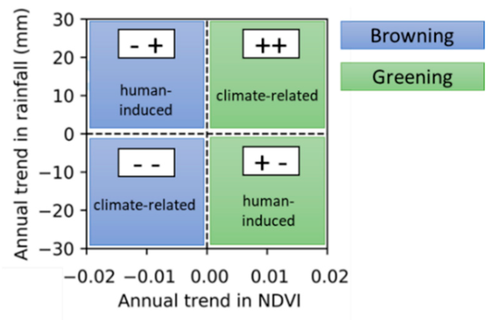
- The examination of spatiotemporal vegetation trends using Landsat time series and to analyse their forcing mechanisms (climate-related vs. human-induced).
- The assessment of the detectability of the impact from typical SLMP interventions on vegetation conditions from the use of relevant remote sensing data sources available at no costs.
2. Materials and Methods
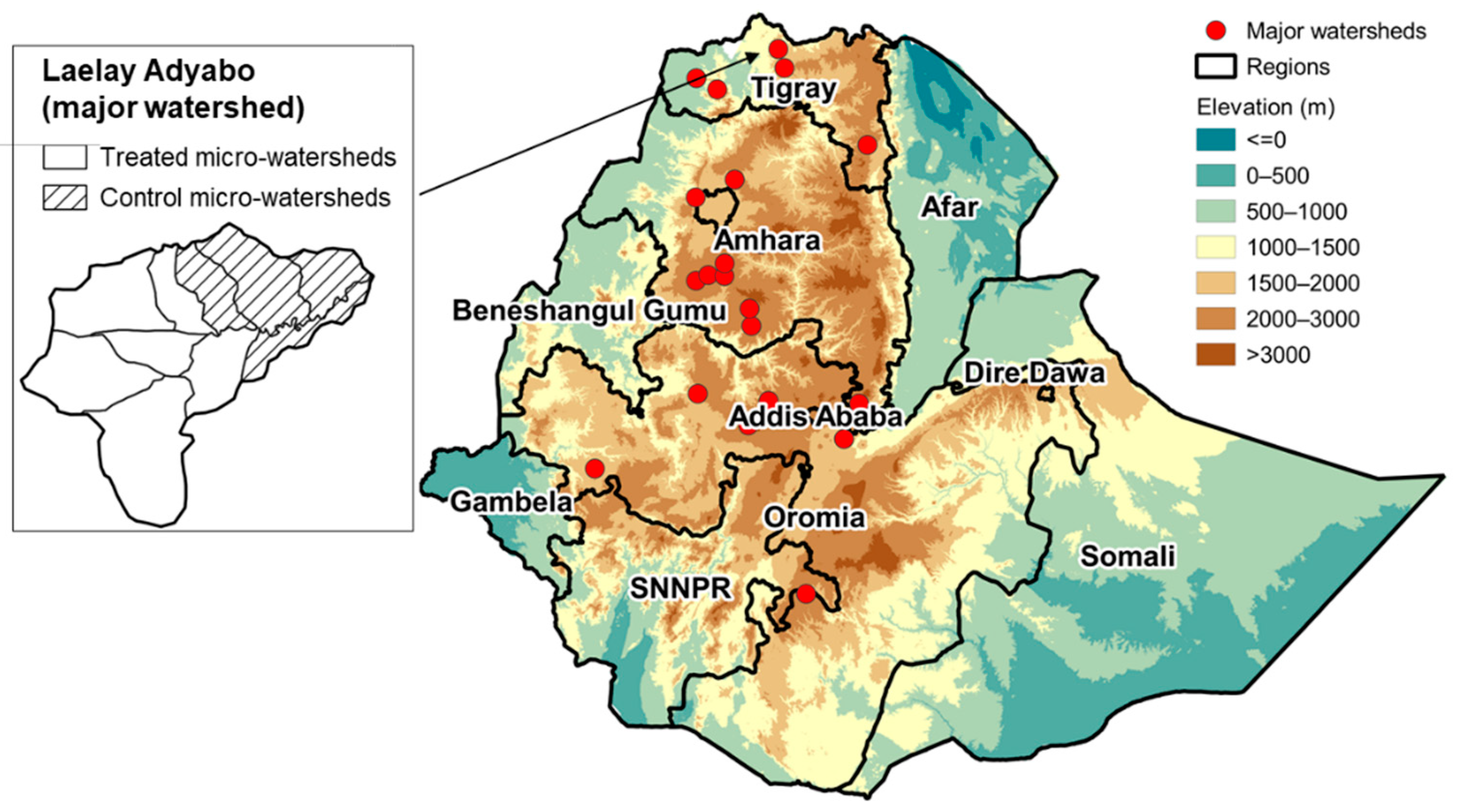
2.1. Study Area
2.2. Data
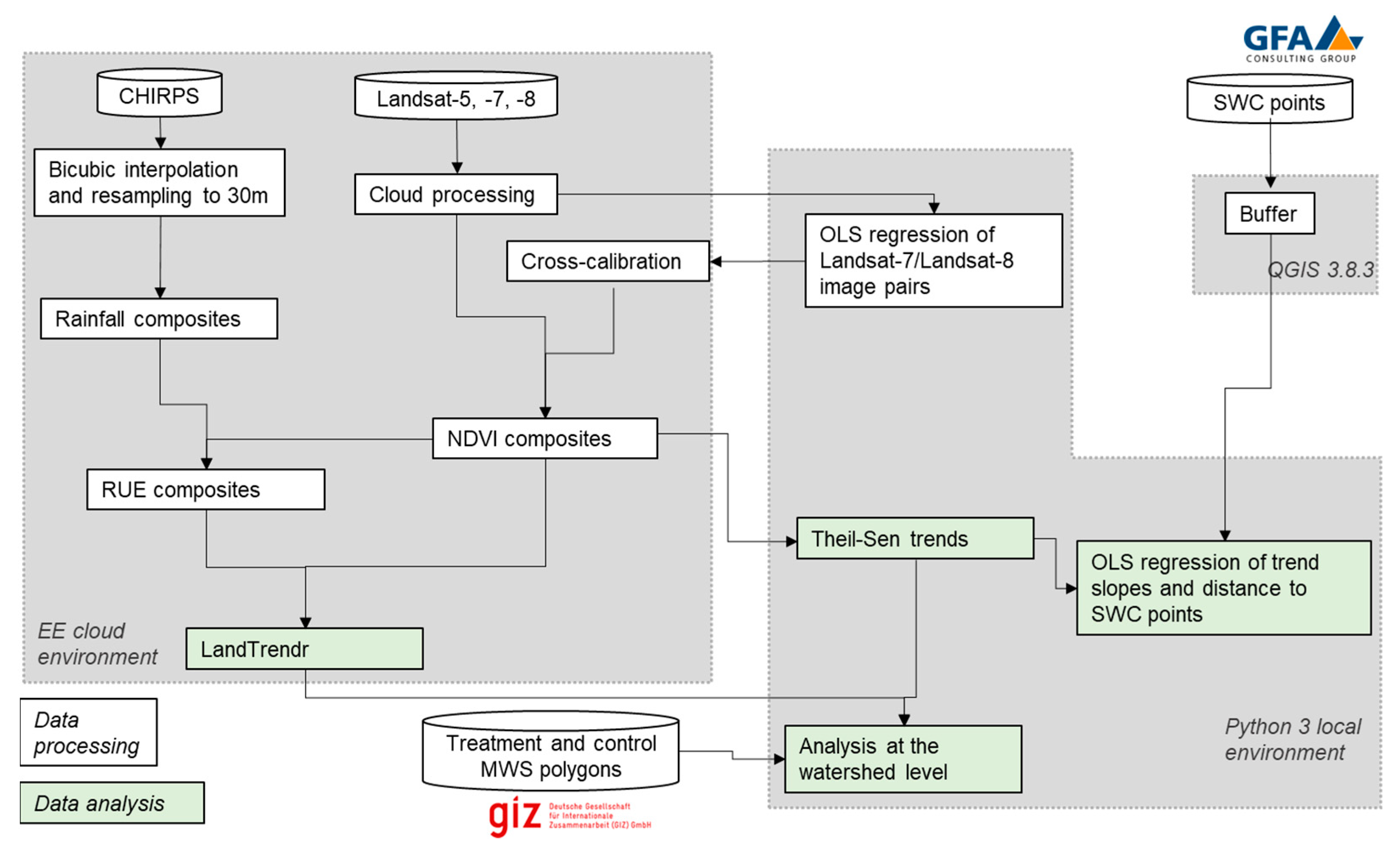
2.3. Methods
2.3.1. Pre-Processing
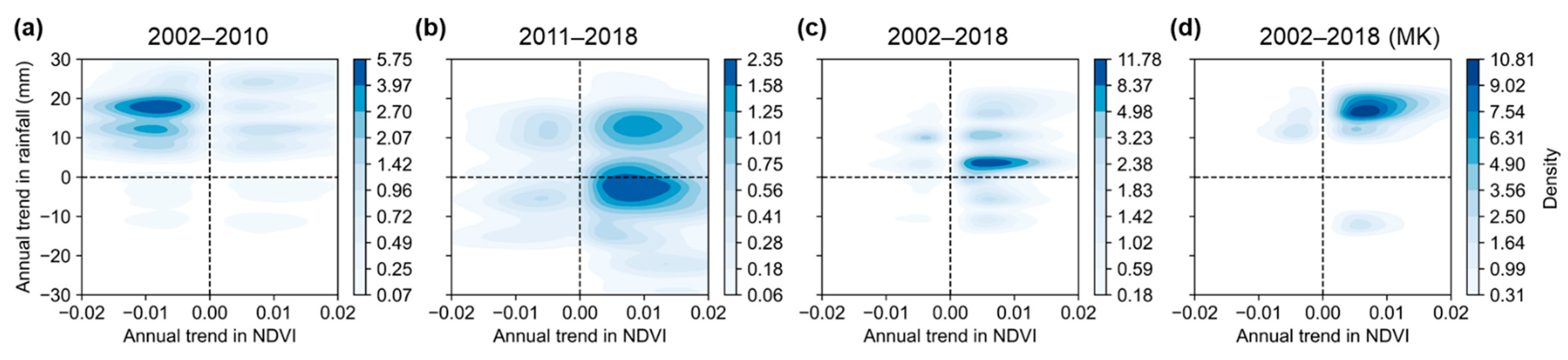
2.3.2. Theil-Sen Regression and Mann-Kendall (MK) Trend Test
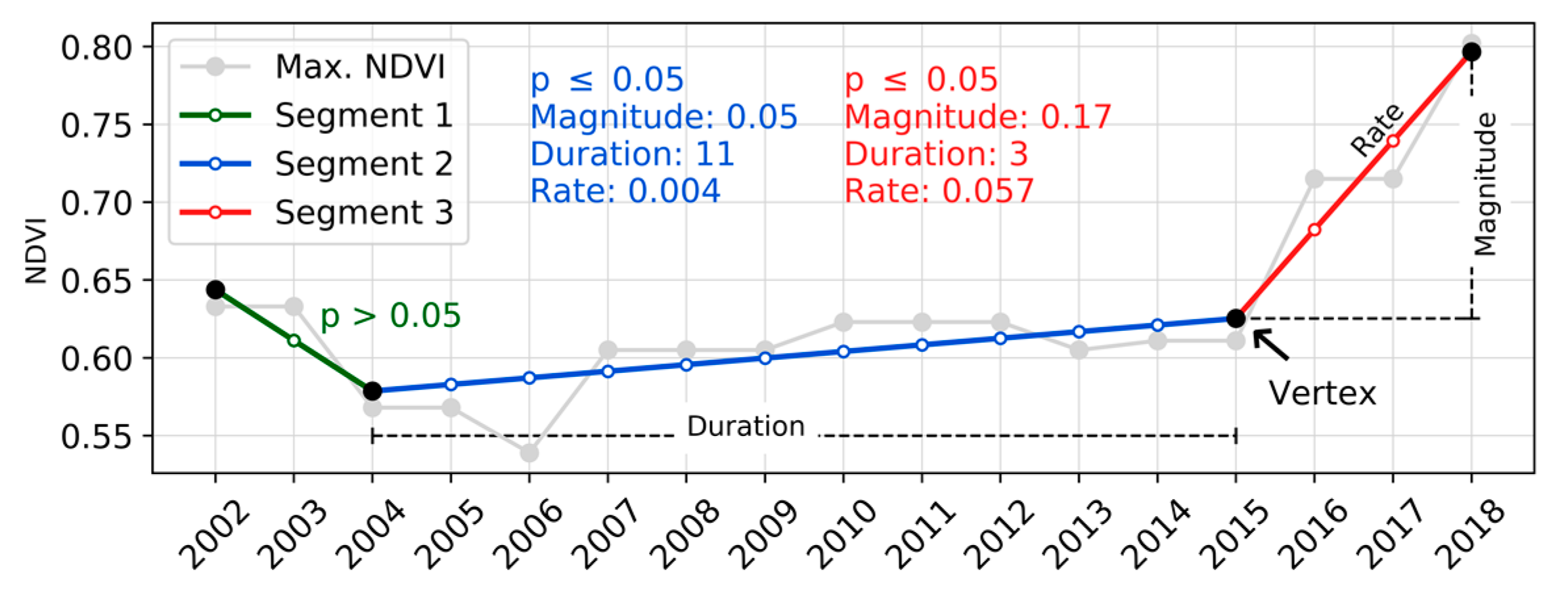
2.3.3. LandTrendr
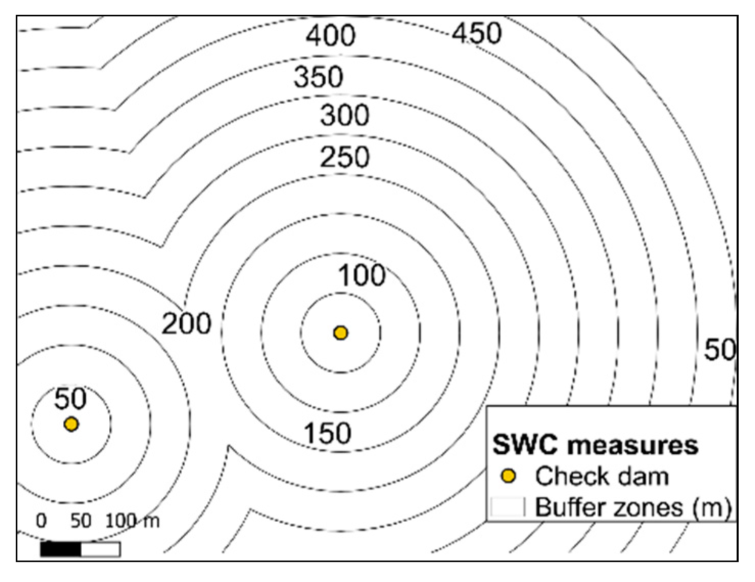
2.3.4. Effect of Soil and Water Conservation (SWC) Measures on Vegetation Trends
3. Results
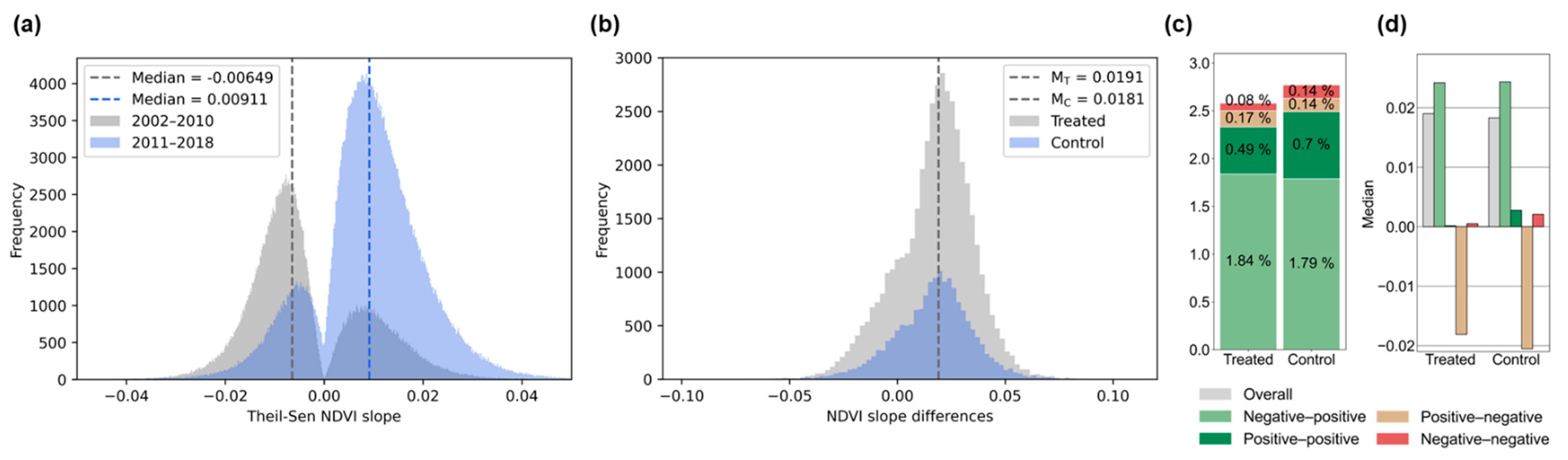
3.1. Treatment and Control Areas
3.1.1. Theil-Sen Trends
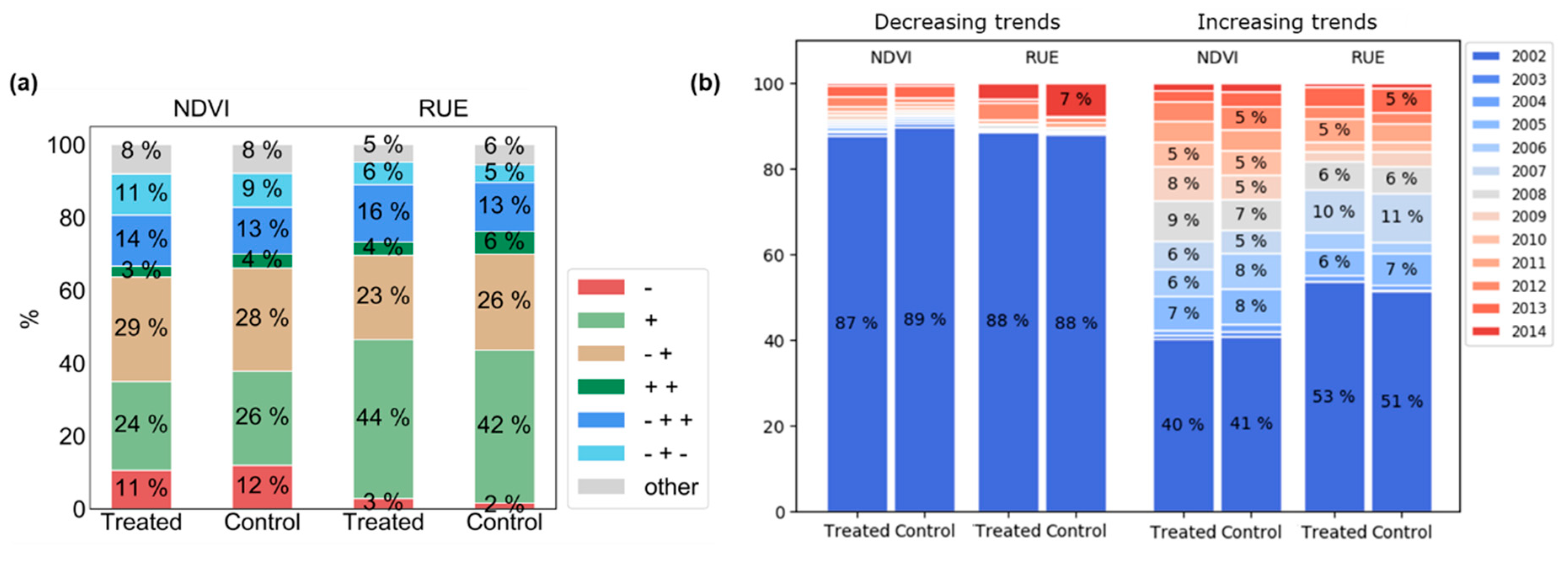
3.1.2. LandTrendr
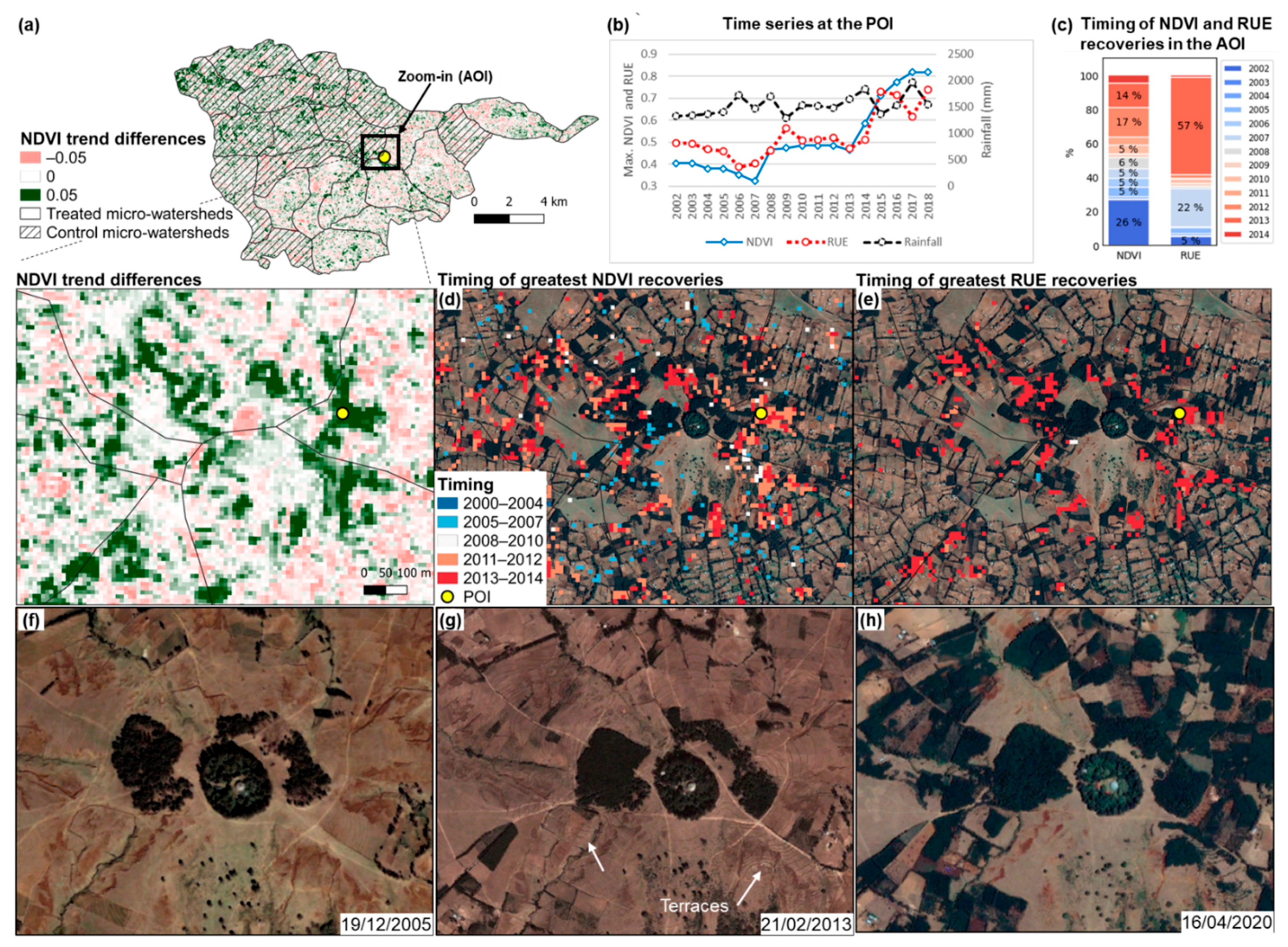
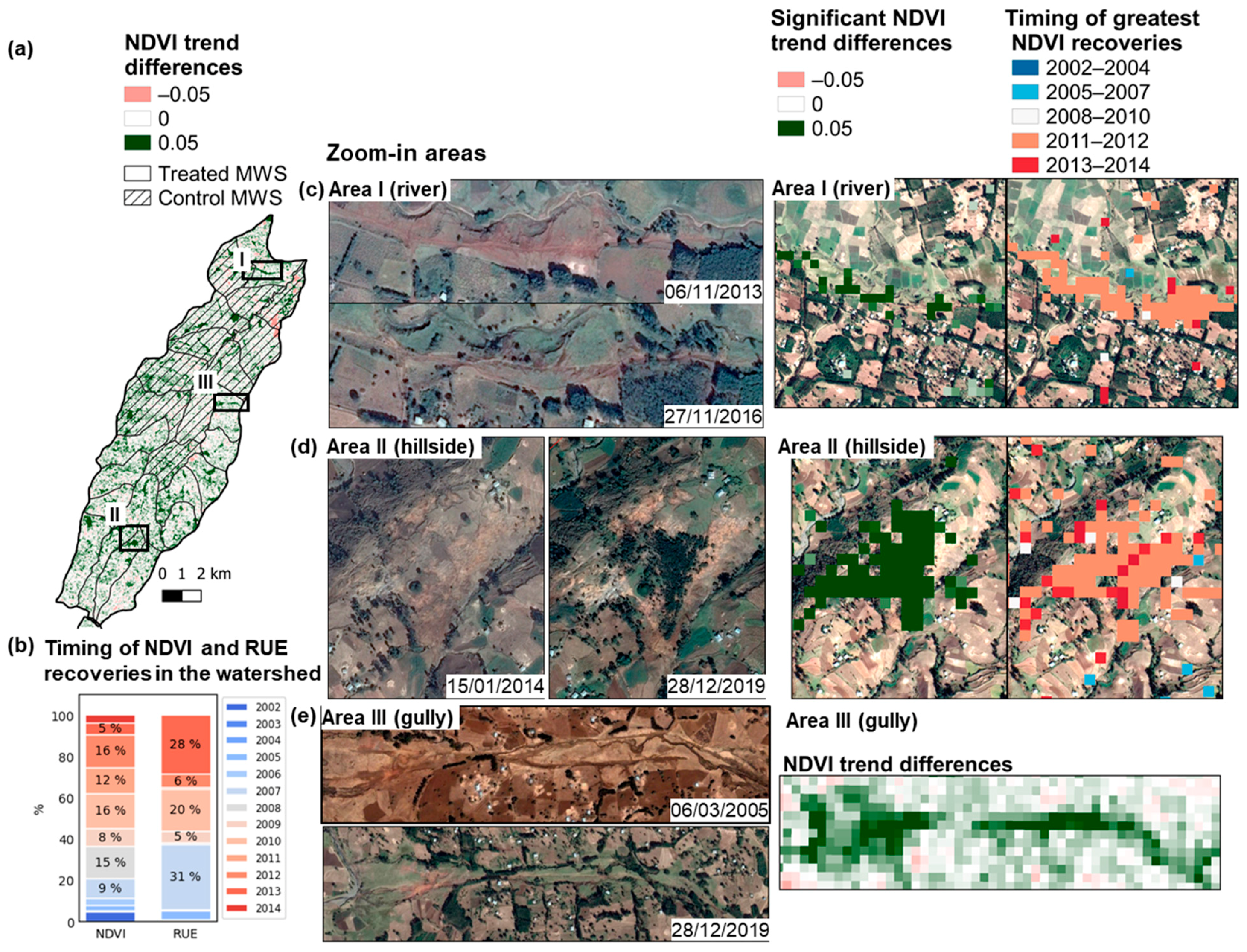
3.2. Visual Inspections of Trends Using Google Earth
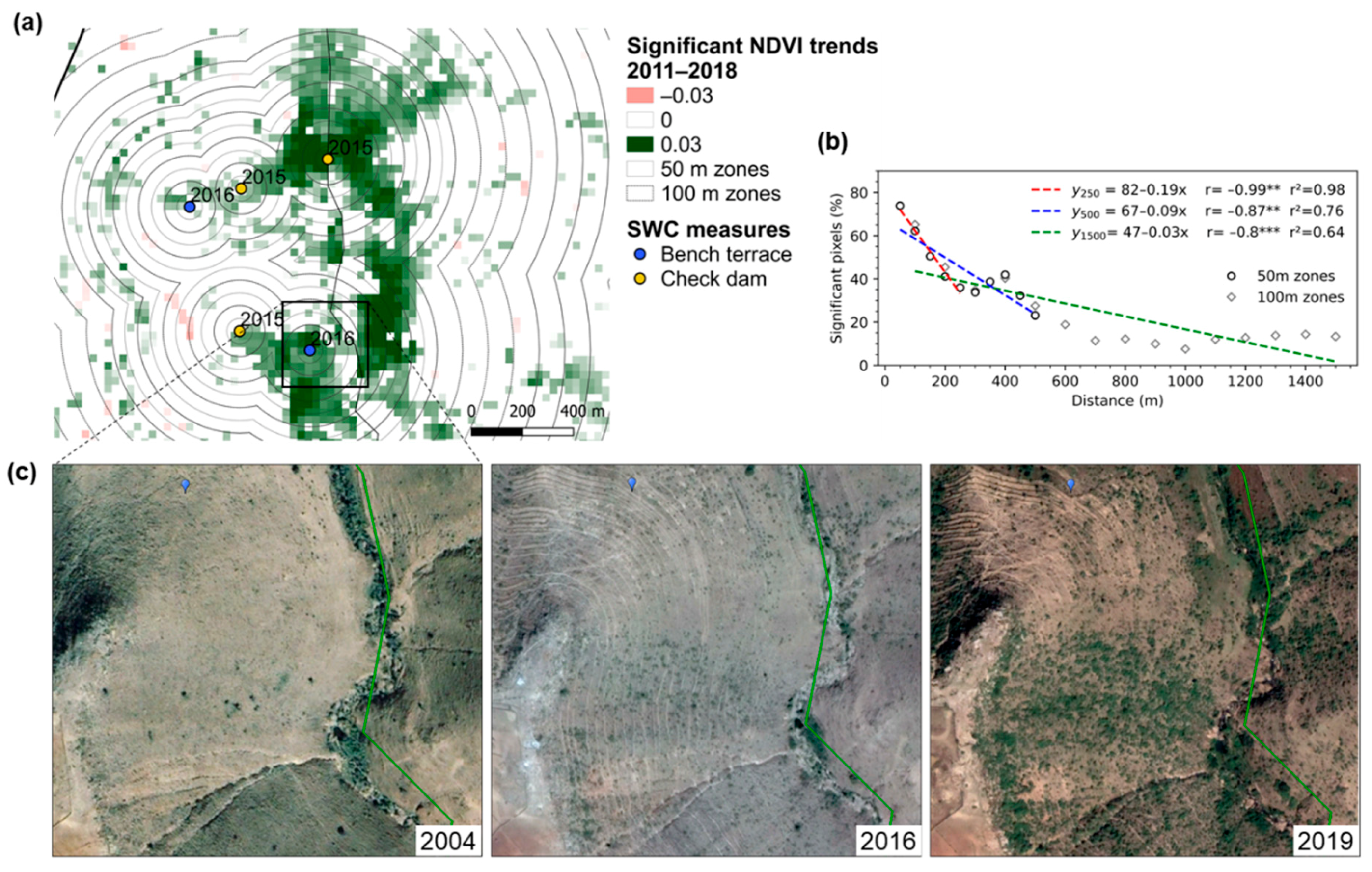
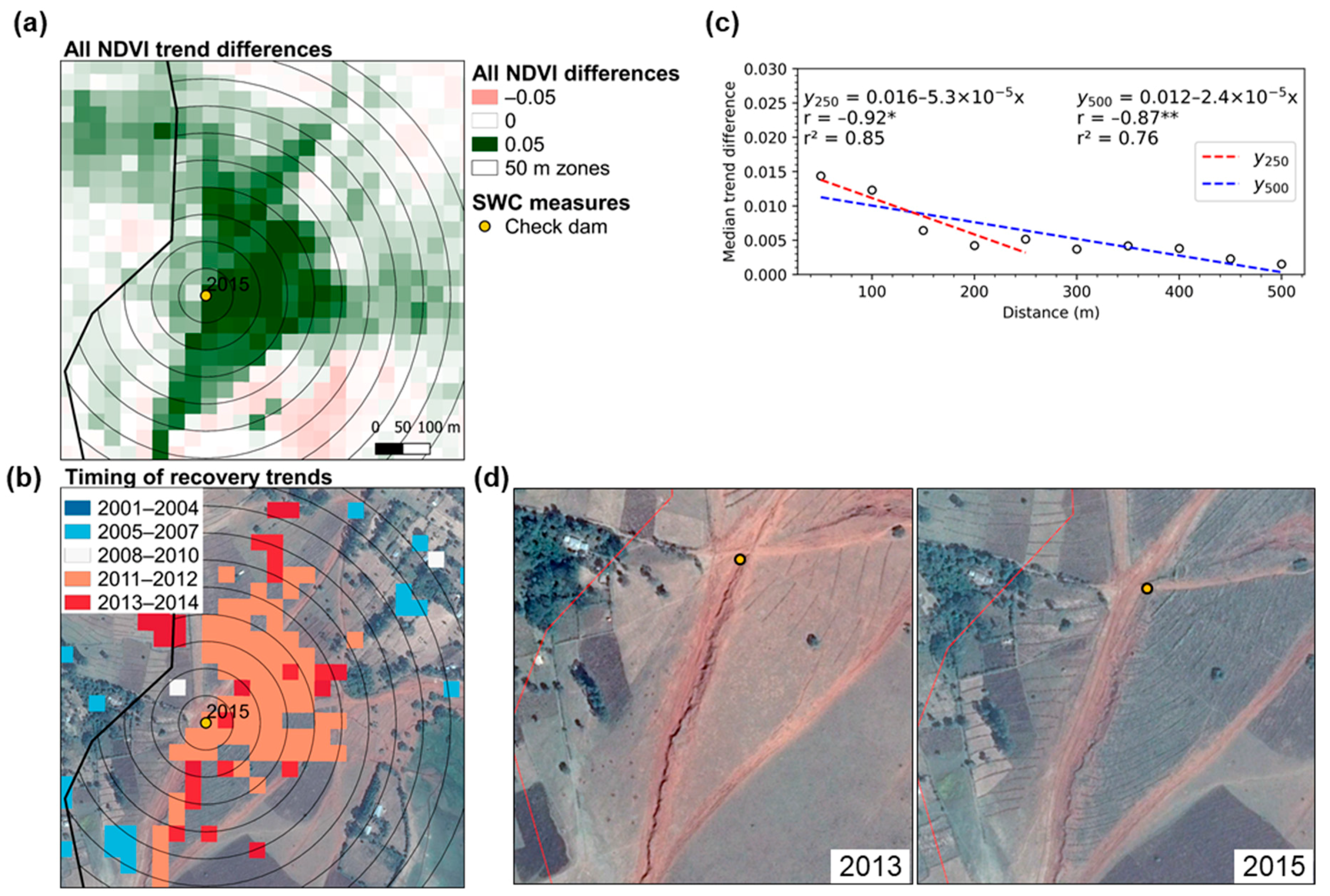
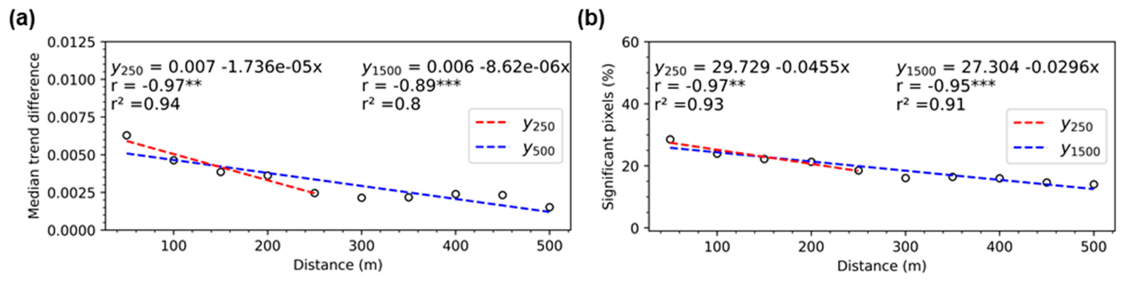
3.3. Effect of SWC Measures on Vegetation Trends
4. Discussion
4.1. Treatment and Control Areas
4.2. Visual Inspections of Trends Using Google Earth
4.3. Effect of SWC Measures on Vegetation Trends
5. Conclusions
Author Contributions
Funding
Institutional Review Board Statement
Informed Consent Statement
Data Availability Statement
Acknowledgments
Conflicts of Interest
Appendix A

| Type of SWC Measure | Purpose | Number of Geolocation Points |
|---|---|---|
| Hillside terraces | Terraces are built to stabilise cultivated land, or to stabilise area. | 11 |
| Check dams | Check dams are obstruction walls constructed at the bottom of a gully, small streams or trenches in order to reduce run-off volume and prevent further widening of the gully channel [62]. These treatment measures are typically combined with revegetation activities to gain higher run-off infiltration into the sediments. | 43 |


| Major Watershed | Treatment | Control | U | ||
|---|---|---|---|---|---|
| N | Median | N | Median | ||
| Laelay Adyabbo | 2091 | 0.0128 | 750 | 0.0116 | - |
| Tahtay Koraro | 6627 | 0.0203 | 604 | 0.0165 | Larger *** |
| Emba Alaje | 1080 | 0.0089 | 34 | −0.0091 | Larger *** |
| Gondar Zuriya | 693 | 0.0137 | 491 | 0.0172 | Smaller ** |
| Takusa | 2182 | 0.0208 | 2526 | 0.0130 | Larger *** |
| West Estie | 5248 | 0.0252 | 1203 | 0.0237 | Larger *** |
| Hagere Mariam | 1060 | 0.0065 | 60 | 0.0164 | Smaller *** |
| Sinan | 2135 | 0.0213 | 1324 | 0.0218 | - |
| Aneded | 3517 | 0.0292 | 2387 | 0.0270 | Larger *** |
| Yilmana Densa | 2539 | 0.0242 | 2204 | 0.0193 | Larger *** |
| Sekela | 2384 | 0.0212 | 972 | 0.0196 | Larger ** |
| Quarit | 2000 | 0.0222 | 1220 | 0.0183 | Larger *** |
| Banja | 2370 | −0.0003 | 2974 | 0.0052 | Smaller *** |
| Ale | 861 | 0.0112 | 131 | 0.0117 | - |
| All watersheds | 43,984 | 0.0190 | 16,880 | 0.0183 | Larger * |

References
- Hannam, I.; Boer, B. Drafting Legislation for Sustainable Soils: A Guide; World Conservation Union: Gland, Switzerland; Cambridge, UK, 2004; ISBN 2-8317-0813-3. [Google Scholar]
- Bai, Z.G.; Dent, D.L.; Olsson, L.; Schaepman, M.E. Proxy global assessment of land degradation. Soil Use Manag. 2008, 24, 223–234. [Google Scholar] [CrossRef]
- Scherr, S.J.; Yadav, S. Land Degradation in the Developing World: Implications for Food, Agriculture, and the Environment to 2020; Paper 14; International Food Policy Research Institute: Washington, DC, USA, 1996. [Google Scholar] [CrossRef]
- United Nations Convention to Combat Desertification (UNCCD). Text of the United Nations Convention to Combat Desertification; 1994. Available online: https://www.unccd.int/sites/default/files/relevant-links/2017-01/UNCCD_Convention_ENG_0.pdf (accessed on 24 March 2021).
- Bekele, W. Economics of Soil and Water Conservation. Theory and Empirical Application to Subsistence Farming in the Eastern Ethiopian Highlands; Wagayehu Bekele: Uppsala, Sweden, 2003; ISBN 9157664331. [Google Scholar]
- Hurni, H. Land Degradation, Famine, and Land Resource Scenarios in Ethiopia; Cambridge University Press: Cambridge, UK, 1993; ISBN 9780511735394. [Google Scholar]
- Berry, L.; Olson, J.; Campbell, D. Assessing the Extent, Cost and Impact of Land Degradation At the National Level: Findings and Lessons Learned From Seven Pilot Case Studies; 2003. Available online: https://rmportal.net/library/content/frame/land-degradation-case-studies-01-overview/at_download/file (accessed on 24 March 2021).
- Lakew, D.; Menale, K.; Pender, J. Land Degradation and Strategies for Sustainable Development in the Ethiopian Highlands: Amhara Region; International Livestock Research Institute: Nairobi, Kenya, 2000; ISBN 9291460907. [Google Scholar]
- Khiari, H.; Jauffret, S.; Walter, S.; Almuedo, P.L.; Lhumeau, A. Land Degradation Neutrality. Transformative Projects and Programmes: Operational Guidance for Country Support; United Nations Convention to Combat Desertification (UNCCD): Bonn, Germany, 2019; ISBN 9789295117655. [Google Scholar]
- World Bank Group. Ethiopia—Second Phase of the Sustainable Land Management Project (English); Washington, DC, USA, 2013. Available online: https://documents.worldbank.org/en/publication/documents-reports/documentdetail/621921468257058351/ethiopia-second-phase-of-the-sustainable-land-management-project (accessed on 24 March 2021).
- Ebabu, K.; Tsunekawa, A.; Haregeweyn, N.; Adgo, E.; Meshesha, D.T.; Aklog, D.; Masunaga, T.; Tsubo, M.; Sultan, D.; Fenta, A.A.; et al. Effects of land use and sustainable land management practices on runoff and soil loss in the Upper Blue Nile basin, Ethiopia. Sci. Total Environ. 2019, 648, 1462–1475. [Google Scholar] [CrossRef]
- Schmidt, E.; Tadesse, F. The impact of sustainable land management on household crop production in the Blue Nile Basin, Ethiopia. L. Degrad. Dev. 2019, 30, 777–787. [Google Scholar] [CrossRef] [Green Version]
- Ali, D.A.; Deininger, K.; Monchuk, D. Using satellite imagery to assess impacts of soil and water conservation measures: Evidence from Ethiopia’s Tana-Beles watershed. Ecol. Econ. 2020, 169. [Google Scholar] [CrossRef] [Green Version]
- Anyamba, A.; Tucker, C.J. Analysis of Sahelian vegetation dynamics using NOAA-AVHRR NDVI data from 1981–2003. J. Arid Environ. 2005, 63, 596–614. [Google Scholar] [CrossRef]
- Eklundh, L.; Olsson, L. Vegetation index trends for the African Sahel 1982-1999. Geophys. Res. Lett. 2003, 30, 1–4. [Google Scholar] [CrossRef]
- Rasmussen, K.; Fensholt, R.; Fog, B.; Vang Rasmussen, L.; Yanogo, I. Explaining NDVI trends in northern Burkina Faso. Geogr. Tidsskr. 2014, 114, 17–24. [Google Scholar] [CrossRef]
- Eckert, S.; Hüsler, F.; Liniger, H.; Hodel, E. Trend analysis of MODIS NDVI time series for detecting land degradation and regeneration in Mongolia. J. Arid Environ. 2015, 113, 16–28. [Google Scholar] [CrossRef]
- Hermans-Neumann, K.; Priess, J.; Herold, M. Human migration, climate variability, and land degradation: Hotspots of socio-ecological pressure in Ethiopia. Reg. Environ. Chang. 2017, 17, 1479–1492. [Google Scholar] [CrossRef]
- Wessels, K.J.; Prince, S.D.; Malherbe, J.; Small, J.; Frost, P.E.; VanZyl, D. Can human-induced land degradation be distinguished from the effects of rainfall variability? A case study in South Africa. J. Arid Environ. 2007, 68, 271–297. [Google Scholar] [CrossRef]
- Helldén, U.; Tottrup, C. Regional desertification: A global synthesis. Glob. Planet. Change 2008, 64, 169–176. [Google Scholar] [CrossRef]
- Symeonakis, E.; Drake, N. Monitoring desertification and land degradation over sub-saharan africa. Int. J. Remote Sens. 2004, 25, 573–592. [Google Scholar] [CrossRef]
- Nicholson, S.; Davenport, M.L.; Malo, A.R. A comparison of the vegetation response to rainfall in the Sahel and East Africa, using normalized difference vegetation index from NOAA AVHRR. Clim. Chang. 1990, 17, 209–241. [Google Scholar] [CrossRef]
- Liou, Y.A.; Mulualem, G.M. Spatio-temporal assessment of drought in Ethiopia and the impact of recent intense droughts. Remote Sens. 2019, 11, 1828. [Google Scholar] [CrossRef] [Green Version]
- Prince, S.D.; Brown De Colstoun, E.; Kravitz, L.L. Evidence from rain-use efficiencies does not indicate extensive Sahelian desertification. Glob. Chang. Biol. 1998, 4, 359–374. [Google Scholar] [CrossRef]
- Fensholt, R.; Rasmussen, K.; Kaspersen, P.; Huber, S.; Horion, S.; Swinnen, E. Assessing land degradation/recovery in the african sahel from long-term earth observation based primary productivity and precipitation relationships. Remote Sens. 2013, 5, 664–686. [Google Scholar] [CrossRef] [Green Version]
- Horion, S.; Prishchepov, A.V.; Verbesselt, J.; de Beurs, K.; Tagesson, T.; Fensholt, R. Revealing turning points in ecosystem functioning over the Northern Eurasian agricultural frontier. Glob. Chang. Biol. 2016, 22, 2801–2817. [Google Scholar] [CrossRef]
- Hein, L.; De Ridder, N.; Hiernaux, P.; Leemans, R.; De Wit, A.; Schaepman, M. Desertification in the Sahel: Towards better accounting for ecosystem dynamics in the interpretation of remote sensing images. J. Arid Environ. 2011, 75, 1164–1172. [Google Scholar] [CrossRef]
- Herrmann, S.M.; Anyamba, A.; Tucker, C.J. Recent trends in vegetation dynamics in the African Sahel and their relationship to climate. Glob. Environ. Chang. 2005, 15, 394–404. [Google Scholar] [CrossRef]
- Ibrahim, Y.Z.; Balzter, H.; Kaduk, J.; Tucker, C.J. Land degradation assessment using residual trend analysis of GIMMS NDVI3g, soil moisture and rainfall in Sub-Saharan West Africa from 1982 to 2012. Remote Sens. 2015, 7, 5471–5494. [Google Scholar] [CrossRef] [Green Version]
- Wulder, M.A.; Masek, J.G.; Cohen, W.B.; Loveland, T.R.; Woodcock, C.E. Opening the archive: How free data has enabled the science and monitoring promise of Landsat. Remote Sens. Environ. 2012, 122, 2–10. [Google Scholar] [CrossRef]
- Zhu, Z. Change detection using landsat time series: A review of frequencies, preprocessing, algorithms, and applications. ISPRS J. Photogramm. Remote Sens. 2017, 130, 370–384. [Google Scholar] [CrossRef]
- Verbesselt, J.; Hyndman, R.; Newnham, G.; Culvenor, D. Detecting trend and seasonal changes in satellite image time series. Remote Sens. Environ. 2010, 114, 106–115. [Google Scholar] [CrossRef]
- De Jong, R.; Verbesselt, J.; Schaepman, M.E.; de Bruin, S. Trend changes in global greening and browning: Contribution of short-term trends to longer-term change. Glob. Chang. Biol. 2012, 18, 642–655. [Google Scholar] [CrossRef]
- Higginbottom, T.P.; Symeonakis, E. Identifying ecosystem function shifts in Africa using breakpoint analysis of long-term NDVI and RUE data. Remote Sens. 2020, 12, 1894. [Google Scholar] [CrossRef]
- Horion, S.; Ivits, E.; De Keersmaecker, W.; Tagesson, T.; Vogt, J.; Fensholt, R. Mapping European ecosystem change types in response to land-use change, extreme climate events, and land degradation. L. Degrad. Dev. 2019, 30, 951–963. [Google Scholar] [CrossRef] [Green Version]
- Griffiths, P.; Kuemmerle, T.; Kennedy, R.E.; Abrudan, I.V.; Knorn, J.; Hostert, P. Using annual time-series of Landsat images to assess the effects of forest restitution in post-socialist Romania. Remote Sens. Environ. 2012, 118, 199–214. [Google Scholar] [CrossRef]
- Grogan, K.; Pflugmacher, D.; Hostert, P.; Kennedy, R.; Fensholt, R. Cross-border forest disturbance and the role of natural rubber in mainland Southeast Asia using annual Landsat time series. Remote Sens. Environ. 2015, 169, 438–453. [Google Scholar] [CrossRef]
- Meigs, G.W.; Kennedy, R.E.; Cohen, W.B. A Landsat time series approach to characterize bark beetle and defoliator impacts on tree mortality and surface fuels in conifer forests. Remote Sens. Environ. 2011, 115, 3707–3718. [Google Scholar] [CrossRef]
- Main-Knorn, M.; Cohen, W.B.; Kennedy, R.E.; Grodzki, W.; Pflugmacher, D.; Griffiths, P.; Hostert, P. Monitoring coniferous forest biomass change using a Landsat trajectory-based approach. Remote Sens. Environ. 2013, 139, 277–290. [Google Scholar] [CrossRef]
- Yin, H.; Prishchepov, A.V.; Kuemmerle, T.; Bleyhl, B.; Buchner, J.; Radeloff, V.C. Mapping agricultural land abandonment from spatial and temporal segmentation of Landsat time series. Remote Sens. Environ. 2018, 210, 12–24. [Google Scholar] [CrossRef]
- Amede, T.; Auricht, C.; Boffa, J.; Dixon, J.; Mallawaarachchi, T.; Rukuni, M.; Teklewold-deneke, T. A Farming System Framework for Investment Planning and Priority Setting in Ethiopia; Canberra, 2017. Available online: https://aciar.gov.au/publication/technical-publications/farming-system-framework-investment-planning-and-priority-setting-ethiopia (accessed on 24 March 2021).
- Zhang, C.; Li, W.; Travis, D. Gaps-fill of SLC-off Landsat ETM+ satellite image using a geostatistical approach. Int. J. Remote Sens. 2007, 28, 5103–5122. [Google Scholar] [CrossRef]
- Funk, C.; Peterson, P.; Landsfeld, M.; Pedreros, D.; Verdin, J.; Shukla, S.; Husak, G.; Rowland, J.; Harrison, L.; Hoell, A.; et al. The climate hazards infrared precipitation with stations—A new environmental record for monitoring extremes. Sci. Data 2015, 2, 1–21. [Google Scholar] [CrossRef] [PubMed] [Green Version]
- Gorelick, N.; Hancher, M.; Dixon, M.; Ilyushchenko, S.; Thau, D.; Moore, R. Google Earth Engine: Planetary-scale geospatial analysis for everyone. Remote Sens. Environ. 2017, 202, 18–27. [Google Scholar] [CrossRef]
- Foga, S.; Scaramuzza, P.L.; Guo, S.; Zhu, Z.; Dilley, R.D.; Beckmann, T.; Schmidt, G.L.; Dwyer, J.L.; Hughes, M.J.; Laue, B. Remote Sensing of Environment Cloud detection algorithm comparison and validation for operational Landsat data products. Remote Sens. Environ. 2017, 194, 379–390. [Google Scholar] [CrossRef] [Green Version]
- Housman, I.W.; Chastain, R.A.; Finco, M. V An Evaluation of Forest Health Insect and Disease Survey Data and Satellite-Based Remote Sensing Forest Change Detection Methods: Case Studies in the United States. Remote Sens. 2018, 10, 1184. [Google Scholar] [CrossRef] [Green Version]
- Roy, D.P.; Kovalskyy, V.; Zhang, H.K.; Vermote, E.F.; Yan, L.; Kumar, S.S.; Egorov, A. Characterization of Landsat-7 to Landsat-8 reflective wavelength and normalized difference vegetation index continuity. Remote Sens. Environ. 2016, 185, 57–70. [Google Scholar] [CrossRef] [Green Version]
- Tian, F.; Fensholt, R.; Verbesselt, J.; Grogan, K.; Horion, S.; Wang, Y. Evaluating temporal consistency of long-term global NDVI datasets for trend analysis. Remote Sens. Environ. 2015, 163, 326–340. [Google Scholar] [CrossRef]
- Chastain, R.; Housman, I.; Goldstein, J.; Finco, M. Empirical cross sensor comparison of Sentinel-2A and 2B MSI, Landsat-8 OLI, and Landsat-7 ETM+ top of atmosphere spectral characteristics over the conterminous United States. Remote Sens. Environ. 2019, 221, 274–285. [Google Scholar] [CrossRef]
- Fensholt, R.; Langanke, T.; Rasmussen, K.; Reenberg, A.; Prince, S.D.; Tucker, C.; Scholes, R.J.; Le, Q.B.; Bondeau, A.; Eastman, R.; et al. Greenness in semi-arid areas across the globe 1981–2007—An Earth Observing Satellite based analysis of trends and drivers. Remote Sens. Environ. 2012, 121, 144–158. [Google Scholar] [CrossRef]
- Fensholt, R.; Horion, S.; Tagesson, T.; Ehammer, A.; Grogan, K.; Tian, F.; Huber, S.; Verbesselt, J.; Prince, S.D.; Tucker, C.J.; et al. Assessment of vegetation trends in drylands from time series of earth observation data. In Remote Sensing Time Series. Remote Sensing and Digital Image Processing; Springer: Cham, Switzerland, 2015; pp. 159–182. [Google Scholar]
- The Federal Democratic Republic of Ethiopia. Ministry of Finance and Economic Development (MOFED). Ethiopia: Sustainable Poverty Reduction Program; 2002. Available online: https://www.imf.org/external/np/prsp/2002/eth/01/073102.pdf (accessed on 24 March 2021).
- Sen, P.K. Estimates of the Regression Coefficient Based on Kendall’s Tau. J. Am. Stat. Assoc. 1968, 63, 1379. [Google Scholar] [CrossRef]
- Kendall, M.G. A New Measure of Rank Correlation. Biometrika 1938, 30, 81. [Google Scholar] [CrossRef]
- McKnight, P.E.; Najab, J. Mann-Whitney U Test. In The Corsini Encyclopedia of Psychology; John Wiley & Sons, Inc.: Hoboken, NJ, USA, 2010; ISBN 9780470479216. [Google Scholar]
- Kennedy, R.E.; Yang, Z.; Gorelick, N.; Braaten, J.; Cavalcante, L.; Cohen, W.B.; Healey, S. Implementation of the LandTrendr algorithm on Google Earth Engine. Remote Sens. 2018, 10, 691. [Google Scholar] [CrossRef] [Green Version]
- Fensholt, R.; Horion, S.; Tagesson, T.; Ehammer, A.; Grogan, K.; TIan, F.; Huber, S.; Verbesselt, J.; Prince, S.D.; Tucker, C.J.; et al. Assessing Drivers of Vegetation Changes in Drylands from Time Series of Earth Observation Data. In Remote Sensing Time Series. Remote Sensing and Digital Image Processing; Springer: Cham, Switzerland, 2015; Volume 22, pp. 183–202. ISBN 978-3-319-15966-9. [Google Scholar]
- Verón, S.R.; Oesterheld, M.; Paruelo, J.M. Production as a function of resource availability: Slopes and efficiencies are different. J. Veg. Sci. 2005, 16, 351–354. [Google Scholar] [CrossRef]
- Suryabhagavan, K.V. GIS-based climate variability and drought characterization in Ethiopia over three decades. Weather Clim. Extrem. 2017, 15, 11–23. [Google Scholar] [CrossRef]
- Zhang, W.; Brandt, M.; Tong, X.; Tian, Q.; Fensholt, R. Impacts of the seasonal distribution of rainfall on vegetation productivity across the Sahel. Biogeosciences 2018, 15, 319–330. [Google Scholar] [CrossRef] [Green Version]
- Mekonnen, M.; Sewunet, T.; Gebeyehu, M.; Azene, B.; Melesse, A.M. GIS and remote sensing-based forest resource assessment, quantification, and mapping in Amhara region, Ethiopia. In Landscape Dynamics, Soils and Hydrological Processes in Varied Climates. Springer Geography; Springer: Cham, Switzerland, 2016; pp. 9–29. ISBN 9783319187877. [Google Scholar]
- Engdayehu, G.; Fisseha, G.; Mekonnen, M.; Melesse, A.M. Evaluation of technical standards of physical soil and water conservation practices and their role in soil loss reduction: The case of debre mewi watershed, north-west Ethiopia. In Landscape Dynamics, Soil and Hydrological Processes in Varied Climates. Springer Geography; Springer: Cham, Switzerland, 2016; pp. 789–818. ISBN 9783319187877. [Google Scholar]


| SWC Type | Buffer Option 1 (250 m) | Buffer Option 2 (500 m) | Buffer Option 3 (1500 m) | ||||||
|---|---|---|---|---|---|---|---|---|---|
| Slope | r | r2 | Slope | r | r2 | Slope | r | r2 | |
| Check dams | −1.7 × 10⁻⁵ | −0.97 ** | 0.94 | −8.60 × 10⁻⁶ | −0.98 *** | 0.8 | −4.00 × 10⁻⁷ | 0.23 | 0.05 |
| Terraces | −2.0 × 10⁻⁷ | −0.02 | 0 | −2.00 × 10⁻⁷ | −0.06 | 0 | −8.00 × 10⁻⁷ | −0.58 * | 0.34 |
| SWC Type | Buffer Option 1 (250 m) | Buffer Option 2 (500 m) | Buffer Option 3 (1500 m) | ||||||
|---|---|---|---|---|---|---|---|---|---|
| Slope | r | r2 | Slope | r | r2 | Slope | r | r2 | |
| Check dams | −0.046 | −0.97 ** | 0.93 | −0.03 | −0.95 *** | 0.91 | −0.007 | −0.79 *** | 0.63 |
| Terraces | −0.035 | −0.64 | 0.42 | −0.029 | −0.87 ** | 0.76 | −0.010 | −0.85 *** | 0.73 |
Publisher’s Note: MDPI stays neutral with regard to jurisdictional claims in published maps and institutional affiliations. |
© 2021 by the authors. Licensee MDPI, Basel, Switzerland. This article is an open access article distributed under the terms and conditions of the Creative Commons Attribution (CC BY) license (http://creativecommons.org/licenses/by/4.0/).
Share and Cite
Barvels, E.; Fensholt, R. Earth Observation-Based Detectability of the Effects of Land Management Programmes to Counter Land Degradation: A Case Study from the Highlands of the Ethiopian Plateau. Remote Sens. 2021, 13, 1297. https://0-doi-org.brum.beds.ac.uk/10.3390/rs13071297
Barvels E, Fensholt R. Earth Observation-Based Detectability of the Effects of Land Management Programmes to Counter Land Degradation: A Case Study from the Highlands of the Ethiopian Plateau. Remote Sensing. 2021; 13(7):1297. https://0-doi-org.brum.beds.ac.uk/10.3390/rs13071297
Chicago/Turabian StyleBarvels, Esther, and Rasmus Fensholt. 2021. "Earth Observation-Based Detectability of the Effects of Land Management Programmes to Counter Land Degradation: A Case Study from the Highlands of the Ethiopian Plateau" Remote Sensing 13, no. 7: 1297. https://0-doi-org.brum.beds.ac.uk/10.3390/rs13071297