
Interpreting Patterns of Concentric Rings within Small Buoyant River Plumes

Remote Sensing Division, U.S. Naval Research Laboratory, Washington, DC 20375, USA
*
Author to whom correspondence should be addressed.
Remote Sens. 2021, 13(7), 1361; https://0-doi-org.brum.beds.ac.uk/10.3390/rs13071361
Submission received: 21 January 2021
/
Revised: 23 March 2021
/
Accepted: 27 March 2021
/
Published: 2 April 2021
(This article belongs to the Special Issue Aerial and Satellite Remote Sensing of Surface Ocean Currents)
Abstract
:High-resolution imagery of small buoyant plumes often reveals an extensive pattern of concentric rings spreading outward from near the discharge point. Recent remote sensing studies of plumes from rivers flowing into the Black Sea propose that such rings are internal waves, which form near a river mouth through an abrupt deceleration of the current, or hydraulic jump. The present study, using numerical simulations, presents an alternative viewpoint in which no hydraulic jump occurs and the rings are not internal waves, but derive instead through shear instability. These two differing dynamical views point to a clear need for additional field studies that combine in-water measurements and time-sequential remote sensing imagery.
1. Introduction
Rivers flowing into the sea add momentum and buoyancy that influence coastal dynamics; and they carry sediment, nutrients, and contaminants, which impact the coastal ecosystem. Where laterally unconfined, the freshwater discharge spreads freely as a plume over the ambient ocean water. An important objective of studies of river plumes, as well as their laboratory analogs, has been to quantify the mixing of the buoyant layer with the ambient fluid [1,2].
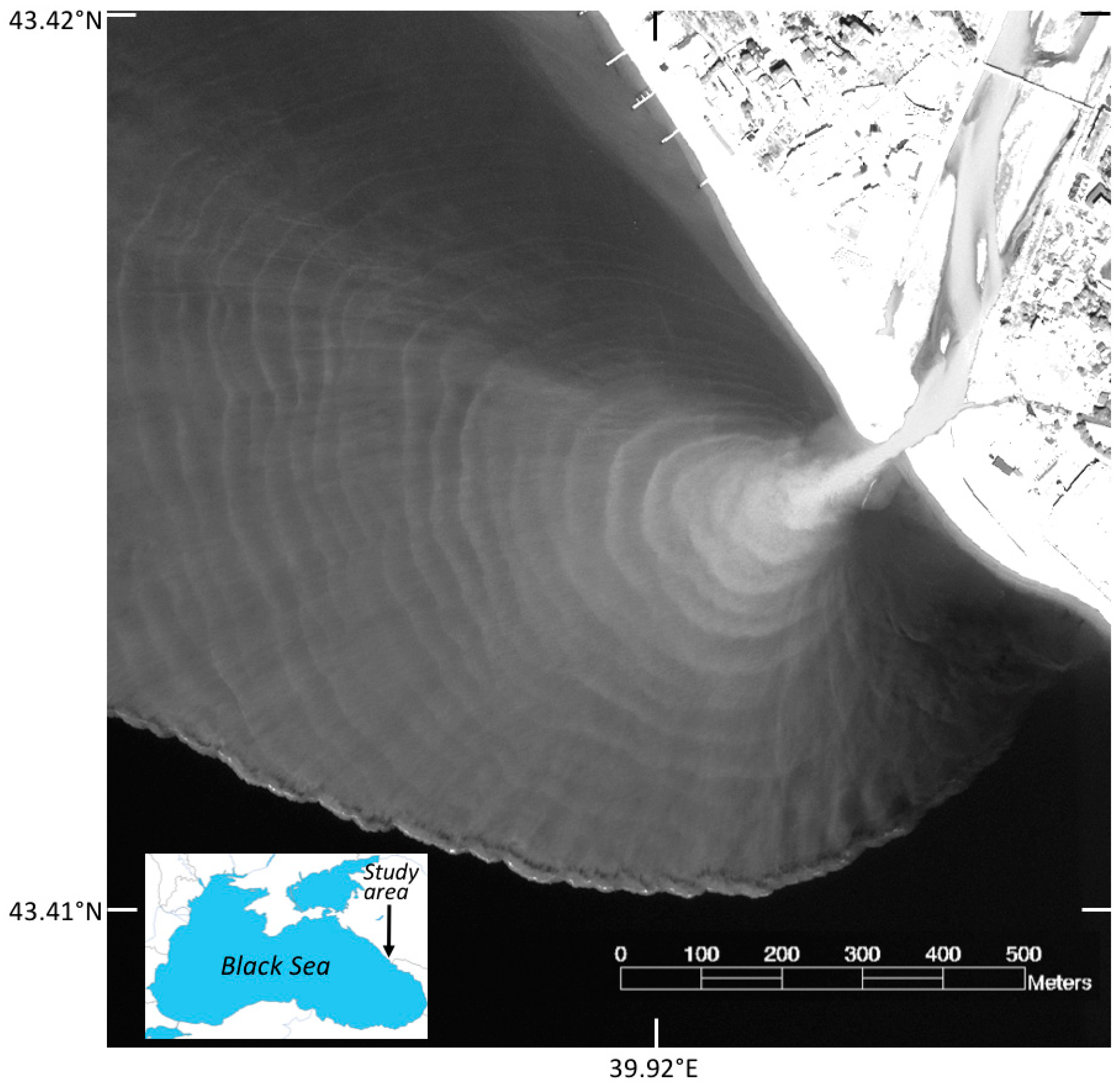
An intriguing feature often found in buoyant plumes from small rivers is a distinctive pattern of nearly concentric bands, or “rings”, which appear to emanate from near the river mouth [3,4,5]. Figure 1 shows an example for the Mzymta River, which is representative of several other small rivers discharging into the Black Sea. Plumes from these rivers show a spacing between consecutive rings in the range of 30 to 60 m [4]. Similar ring-like patterns have been found to occur in a near-surface discharge of heating water from an electric power-generating plant [6]. In the literature, such features have been referred to as internal bands, fronts, and bores (e.g., reference [2]).
Recent remote sensing studies of plumes like the Mzymta’s claim such features within a plume are high-frequency internal waves that propagate away from a source region near the river mouth [4,5,7,8]. Note that this is distinct from internal waves that can form ahead of the plume, if the ambient water is stratified [9,10,11]. The explanation given for the origin of the internal waves is that as the river flows into the coastal sea it abruptly decelerates through a quasi-stationary hydraulic jump, and that the internal waves are generated through an assumed oscillation of this jump. No explicit theoretical formulation, however, is provided for this mechanism. It is also assumed these internal waves significantly increase mixing of the plume with underlying ambient sea water; but there is, as yet, no evidence to confirm this. It is fair to say, therefore, that, while the phenomenon may be widespread [4], the physical mechanisms and potential environmental consequences are not well understood.
The objective of the present report is to demonstrate, using a numerical model, that ring-like features resembling those in Figure 1 can be simulated, but that such rings are not internal waves, nor do they derive from an abrupt transition in the plume velocity field. The results are thus incompatible with the hypothesis stated above, and this has implications for interpreting not only remotely sensed imagery of the river plume, but also measurements of water-column hydrography. These differing dynamical views point to a clear need for additional studies that combine in-water measurements and time-sequential remote sensing imagery.
2. Materials and Methods
2.1. Background
The prototype for this study is the plume formed by the Mzymta River. The Mzymta River, which flows through the western edge of the Caucasus mountains, discharges into the eastern Black Sea about 25 km southeast of the city of Sochi, Russia. There the river is characterized by relatively high speed, but small vertical extent and volume. The Mzymta discharge rate is, however, highly variable with monthly means ranging from 20 to 120 m3 s−1 [5]. During periods of significant discharge, river speed (either measured directly or inferred from discharge gauge data) is in the range of about 1 to 2 m s−1 [5,12]; water depth at the river mouth is nominally 1 to 1.5 m; and river width near the mouth averages about 40 m. The small length scale but large velocity of the Mzymta discharge gives rise to a near-field supercritical flow [4], meaning that the plume water velocity exceeds the speed of a linear internal wave phase speed. Within the near field, the plume is dominated by the inertia of the discharge and behaves much like a turbulent buoyant jet. Previous studies suggest that a small river plume will transition from supercritical near field to subcritical far field gradually and over a significant distance (on the order of a kilometer) from the river mouth [1]. For the Mzymta, the near field can extend as far as 1 to 2 km from the river mouth, beyond which the dynamics are dominated by wind stress and the effect of Earth’s rotation [12].
The Mzymta carries out to sea large amounts of silt and organic suspended matter, resulting in a turbid plume that is easily detectible in ocean color satellite imagery. The WorldView-3 satellite image shown in Figure 1 may be the best highest-resolution data of the plume that exists currently. It was acquired in early spring (4 April 2017), during a discharge of approximately 60 m3 s−1 (Figure 4 in reference [4]). Shown are data from band 3 (green: 518 to 586 nm wavelengths), as it was found to have the greatest dynamic range, or signal contrast, and thus best highlights key features of the plume. The discharge can be seen to have an initial width of about 25 m at the river mouth. The plume extends 780 m from the mouth (in the direction normal to shore), and the signal level decays with distance with an e-folding scale of about 300 m. A gradual turn of the plume toward the north may indicate a transition to far-field dynamics. The seaward-most extent of the plume is marked by a distinct front and narrow scum line. The plume front displays a lobe-cleft structure that is characteristic of gravity current-like geophysical flows [13,14]. Lobes protrude seaward from the front, while clefts are indentations in the frontal edge. In Figure 1, successive lobes and clefts are spaced most commonly in the range of 40 to 80 m. On the plume side of the front, displaced by about 15 m, lies an approximately parallel, or “companion”, dark band. This band may indicate an upwelling of relatively clear water in the rear of the frontal head, where the plume protrudes downward behind the surface front (for example, reference [15]). Rings in Figure 1 appear relatively bright, suggesting they are regions where the turbid plume water is locally deeper than the water between rings. Individual rings can extend coherently over a wide azimuth; some appear to either split or merge with others. Over the bulk of the plume, the ring spacing averages 39 m (±9 m). Rings are more finely spaced, however, in the plume area northwest of the river mouth. The rings appear to emanate from a source region located 100 to 200 m from the river mouth and extending 25 to 100 m alongshore [4].
There is, as yet, no WorldView stereo imagery of the Mzymta plume from which one might deduce currents (for example, [16]). But pairs of images from Sentinel-2 and Landsat 8 satellite overpasses that were closely spaced in time have been used by Osadchiev [4] to deduce information about the ring features. Under the assumption that the features represent internal waves, he reports wavelengths in the range of 30 to 60 m, phase speeds of 0.45–0.65 m s−1, and wave periods (that is, wavelength divided by phase speed) of 65 to 90 s [4,17]. We posit that what was actually measured was the advection speed of the features; hence the period should be interpreted instead as the time interval between generation of each successive ring (c.f., Section 3.2).
In-water data for the Mzymta plume are sparse. The most relevant hydrographic measurements were made by Osadchiev [4], on a day (29 May 2014) when a LANDSAT-8 pass revealed plume structure similar to that of Figure 1. The measurements are comprised of eight “tow-yo” profiles made in water depths of 7 to 8 m and over a horizontal distance of 50 m, beginning about 150 m from the river mouth; hence, the data were collected within the apparent source region of the ring features. While six of the profiles showed the expected structure of a plume confined to the upper meter or so of the water column, profiles 1 and 3 were anomalous in that they showed low-salinity plume water penetrating downward over nearly the entire depth of the water column. These two localized, downward penetrations of plume water were interpreted as evidence of a hydraulic jump.
2.2. Model
The plume is modeled in three-dimensions using non-hydrostatic and non-rotational dynamics. We use the OpenFOAM solver TwoLiquidMixingFoam, run as a large-eddy simulation. OpenFOAM is a free, open-source library of source code for solvers and utilities [18]. A large-eddy simulation resolves spatial scales from the domain size down to a filter size ∆; effects of smaller scales must be modeled. In this study, turbulent effects on scales smaller than ∆ are modeled using a k-equation eddy viscosity model. The model solves a turbulence kinetic energy equation, yielding the sub-grid-scale turbulent kinetic energy, 𝑘sgs. A sub-grid-scale eddy viscosity, 𝜈sgs, is then computed as 𝜈sgs = Ck (𝑘sgs)1/2 ∆, where Ck is a model constant set to a value of 0.094. The dissipation term in the turbulence kinetic energy equation is given by 𝜖 = C𝜀 k3/2/∆, where C𝜀 = 1.048 is another model constant. The quantity 𝜖 thus provides an estimate of the dissipation rate of turbulent kinetic energy; hence, of vertical mixing. As the focus of the model is the near field of the river plume, neglect of Earth’s rotation is justified.
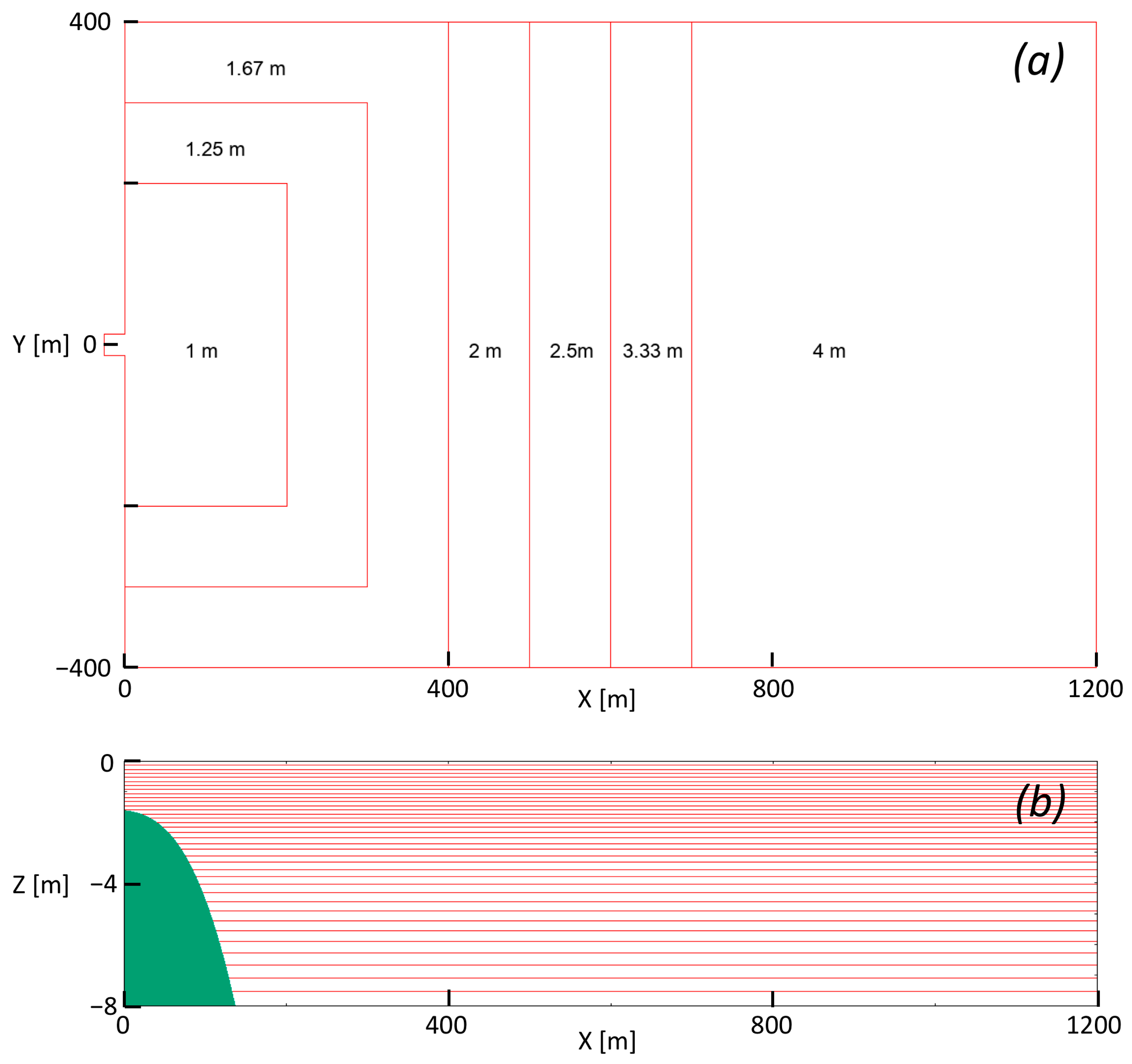
Model geometry is shown in Figure 2. A notch at y=0, x< 0 represents the river inflow, which has a width W0 = 26 m and depth H0 =1.6 m. For 0 < x < 137 m, the bottom depth is specified as z = −1.6 − 1.5 × 10⁻⁶ (x + 25)3; for x > 137 m the bottom is fixed at 8-m depth; there is no depth variation in the alongshore (y) direction. In reality, the ocean floor continues to deepen offshore, reaching 100 m within 1 to 2 km of the river mouth. The bottom boundary is modeled as no slip, using a wall function to adjust the bottom-layer eddy viscosity. The sea surface is assumed to be a rigid lid. Boundary conditions of slip, zero-gradient are used on the two across-shore boundaries, and a zero-gradient condition is applied at the offshore boundary.
Grid resolution varies both horizontally and vertically (Figure 2). Near the inflow the horizontal resolution (∆x, ∆y) is 1 m; it becomes progressively coarser with increasing x. In the vertical direction, z, resolution is greatest near the sea surface, where 12 layers cover 1.6 m; another 24 layers, each successively 5.57% larger, cover the remaining 6.4 m; the thickest layer is 46 cm. The filter length scale ∆ is taken as proportional to the cube root of the cell volume: ∆ = C∆ (∆x ∆y ∆z) 1/3, where C∆ is a constant. In this work, we used C∆ = 0.2, as much larger values were found to damp the formation of rings, while smaller values resulted in an incoherent flow field. The model time step ∆t was varied to limit the Courant number at 0.4; the mean value of ∆t was 0.14 s. A model run typically ends when the plume intersects an across-shore boundary.
The river, or inflow, water has a density 𝜌1= 1000 kg m−3, and the ambient sea water a density 𝜌2= 1017 kg m−3 [17,19,20]; thus, the inflow reduced gravity g0′ = g (𝜌2 − 𝜌1)/𝜌2 = 0.1640 m s−2, where g = 9.81 m s−2 is the gravitational acceleration constant. In portraying the modeled density field in the results section, we use a normalized density 𝜌⁎ = (𝜌 − 𝜌1)/(𝜌2 − 𝜌1), so that a value of zero corresponds to river water, and a value of one to sea water. The base-case simulation uses a constant inflow velocity U0 = 1.5 m s−1. This value was chosen as it falls in the middle of the range of Mzymta River flow speeds (Section 2.1). The inflow freshwater discharge rate is thus U0 W0 H0 = 62.4 m3 s−1, which is comparable to the discharge at the time of Figure 1. The inflow conditions can be characterized in terms of an inflow Froude number, Fri = U0/sqrt (g0′ H0) = 2.93. A value of Fri > 1 indicates supercritical inflow.
3. Results
3.1. Spatial Structure
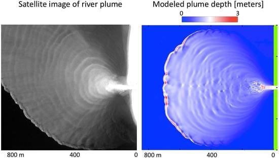
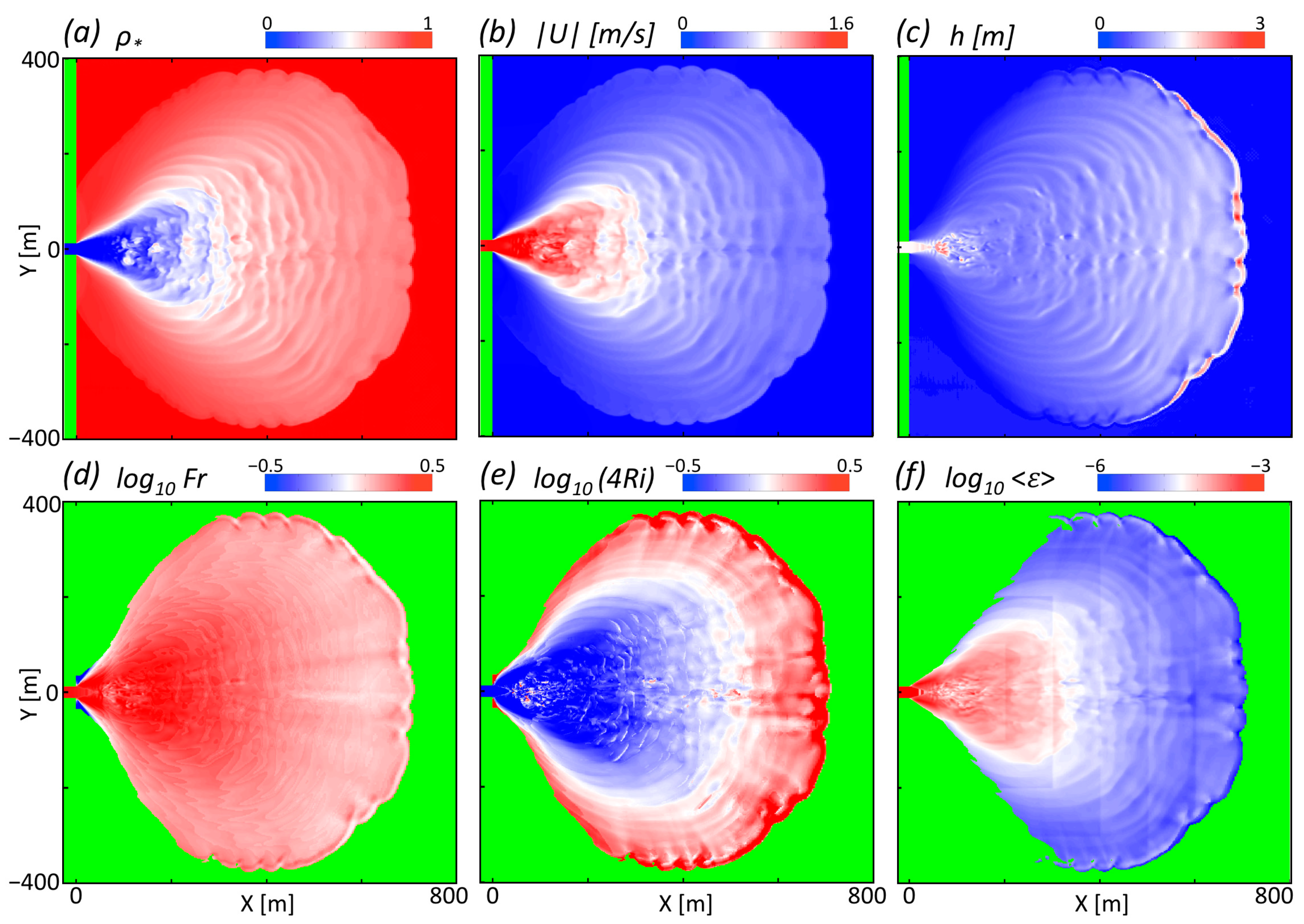
Representative model results are shown in Figure 3, corresponding to a time of 1630 s (27.2 min) after the start of the simulation. By this time the plume has expanded to a size of 710 by 750 m in the across- and along-shore directions. Ring-like features appear in the surface density field as narrow bands of relatively buoyant fluid (Figure 3a); in the surface velocity as bands of locally higher speed (Figure 3b); and as bands of increased plume depth h (Figure 3c). The model rings resemble those in satellite imagery of the Mzymta plume. Rings appear over nearly all azimuth directions, and, as will be demonstrated below, move continuously offshore and toward the plume front. The rings appear to emanate from a source region, approximately 75 to 175 m from the model river mouth and having an alongshore extent of about 80 m; this is comparable to estimates derived from satellite imagery (Section 2.1). The spacing between successive rings in the model is about 37 m (±9 m), representing an average over a central, 20°-azimuth sector. This is comparable to the mean ring spacing of 39 m in the satellite image in Figure 1. Model rings are more closely spaced well off the plume centerline, similar to Figure 1.
Other characteristics of the plume are also in reasonable agreement. The modeled fields of surface density and speed decay approximately exponentially with radial distance from mouth, with an e-folding scale of about 325 m; this is comparable to the turbidity decay scale of the Mzymta plume (Section 2.1). The model plume front has a lobe-cleft structure (dominant spacing of 40 to 70 m) that resembles that in Figure 1. The model result for plume depth (Figure 3c) shows the expected frontal head structure: a narrow, leading band where with the plume is deepest; and a narrow, trailing area that is (persistently) shallow and resembles the companion dark band in the satellite data (Figure 1). One apparent difference between the simulation and imagery is that the model inflow begins spreading laterally almost immediately, while the imagery shows little initial spreading. This is in large part because the density and velocity plots in Figure 3 show surface fields, while the imagery is showing depth-integrated backscattered light. When model results are integrated over a plausible optical penetration depth of 1 m, the spreading is much reduced so that the shape of the discharge resembles that of the depth field in Figure 3c.
The dynamical character of the plume can be revealed by examining two parameters: the Froude number Fr = U/(g’ h)1/2, where and U and h are local values of plume depth and velocity, respectively, g’ is the local reduced gravity; and the Richardson number, Ri = −(g/𝜌) 𝜕𝜌/𝜕z/(𝜕U/𝜕z)2, evaluated at the depth where |𝜕𝜌/𝜕z| is maximum. The value of Fr can be seen (Figure 3d) to exceed one almost everywhere, indicating that at this evolutionary stage the entire plume is supercritical and can thus be considered a near-field buoyant flow. In particular, there is no evidence of an abrupt transition to sub-critical flow close to the river mouth; this is distinctly different from the view of references [4,5,7,8]. And because the plume is supercritical nothing that occurs downstream can affect the creation of rings that is occurring upstream; hence, modeled rings continue to form and evolve in a similar way throughout a simulation. In the plot of Richardson number (Figure 3e), shades of blue correspond to values of Ri less than the critical value of 0.25. Values of Ri < 0.25 indicate regions of the flow field that are susceptible to Kelvin–Helmholtz shear instability (KHI). Ri falls significantly below its critical value over the innermost part of the plume (see later Section 3.3).
The spatial distribution of kinetic energy dissipation rate 𝜖 (Figure 3f) provides an indication of where turbulent mixing is occurring within the plume. Mixing is thus predicted to be highest (nearly 10−3 m2 s−3) in the source region of the rings, where values of Ri are smallest, and to decay strongly with increasing radial distance. This is consistent with mixing in river plumes being dominated by stratified shear-flow instabilities [1]. Rings have higher dissipation rates than do plume areas between rings. This provides some evidence that ring features enhance vertical mixing between the plume and the underlying sea water. Figure 3c shows that, away from the source region, the plume thickens with radial distance, the rate of increase being approximately constant over radial distances of 200 to 550 m. This thickening is evidence of turbulent entrainment of lower-layer fluid into the plume.
3.2. Evolving Nature of the Plume
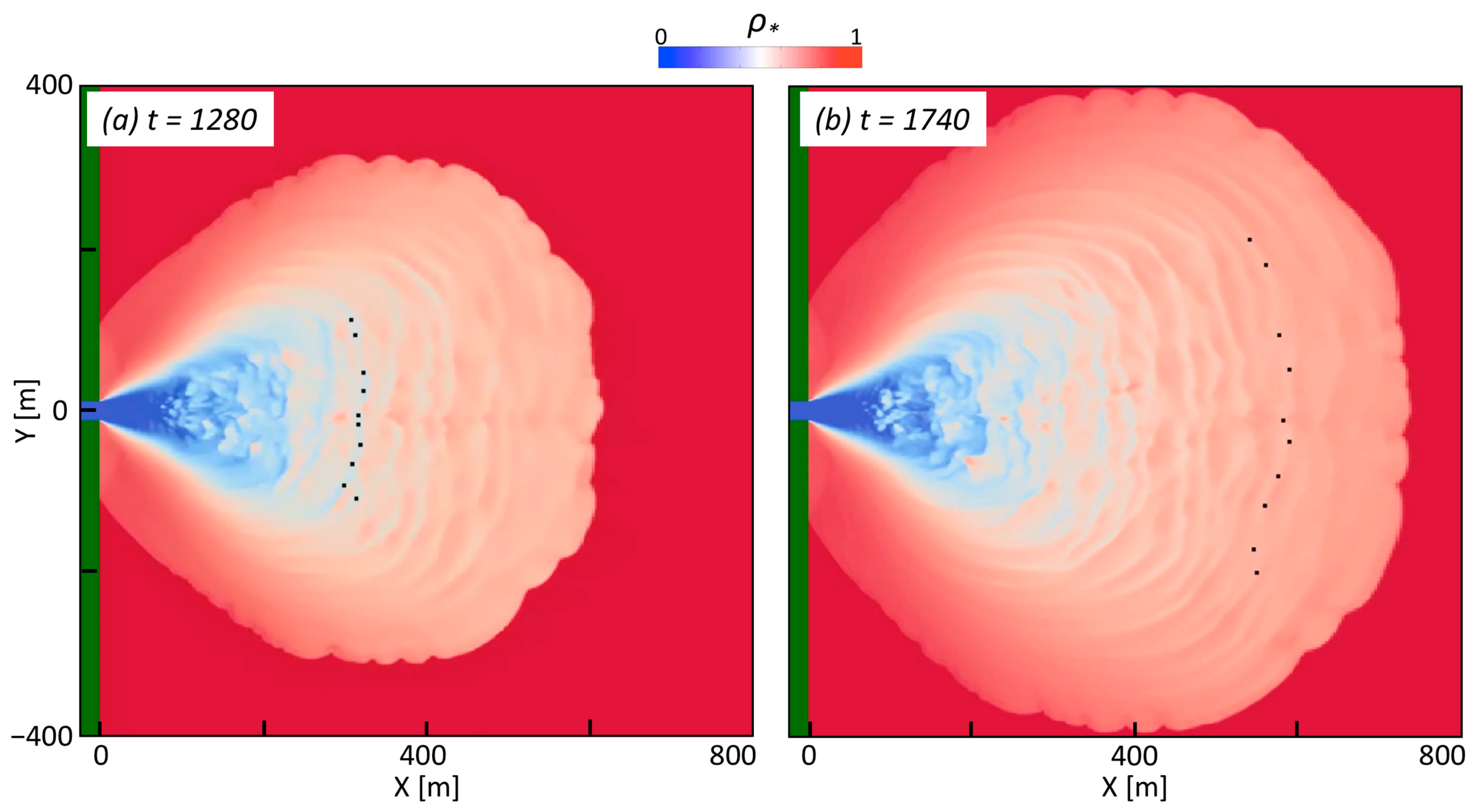
Rings produced by the model are not internal waves. This can be demonstrated by tracking virtual surface particles chosen to lie within a particular ring at some initial time, as shown in Figure 4a. Subsequent particle positions were determined by computing their Lagrangian displacements, using the surface velocity field at each model time step. An animation of the evolving density field (Figure S1) shows the particle positions over a time period of 460 s, the final time being shown in Figure 4b. Over time, the chosen particles advect radially and, as a group, stretch-out azimuthally. But, throughout, the particles remain within the same ring features. If those features were internal waves, they would propagate through the plume and leave the particles behind them. That does not occur; thus, the rings are material features.
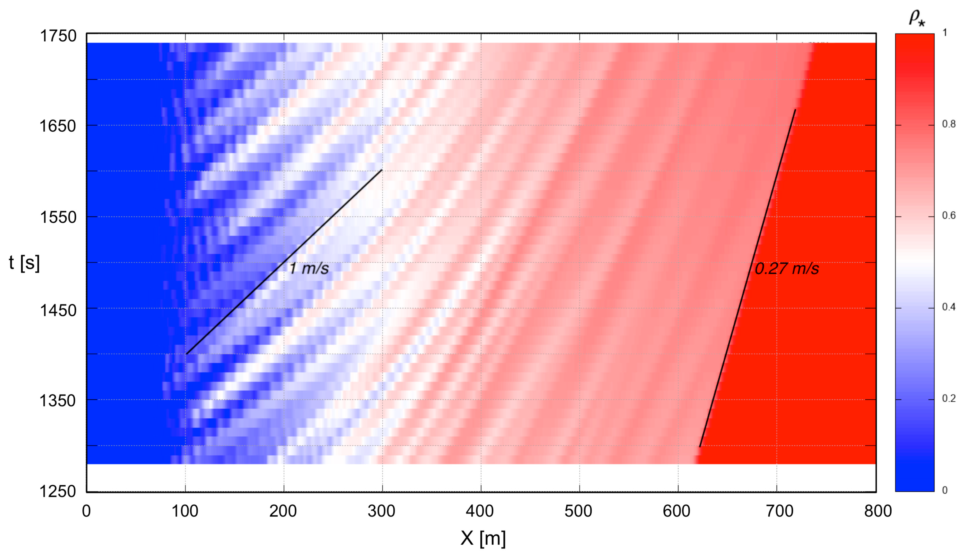
Rings move continuously offshore and toward the plume front. This is illustrated through a Hovmöller diagram (Figure 5) generated from the centerline surface density. The diagram shows a pattern of blue-white streaks (that is, locally more buoyant water) inclined from the lower-left toward the upper-right, and which represents the offshore movement of the rings. Rings move at 1 m s−1 near their source region (at x ~ 100 m), but slow with increasing offshore distance until reaching the plume front, which itself advances into ambient water at a steady radial speed of 0.27 m s−1. The rings thus advance faster than the plume front; but they never move beyond the plume front, which is consistent with Figure 1 and other satellite imagery [4,5]. The range of predicted ring speeds is consistent with that deduced from satellite imagery by Osadchiev (Section 2.1). Inshore of x~300 m, the period between successive rings in Figure 5 is about 60 s. While this value is comparable to internal wave periods reported for the Mzymta plume [4,17], our interpretation is as an estimate of the time interval at which rings are generated within the source region. Note that the plume translation speed is often described in terms of the long-wave internal wave phase speed c = (g’ h)1/2, which can be calculated using the Fr and U data in Figure 3. Near the front, c = 0.28 ± 0.02 m s−1, which is not significantly different from the speed of frontal advance derived from Figure 5. The continuous offshore advance of the plume would, of course, in the real world be arrested by far-field dynamics (Section 2.1).
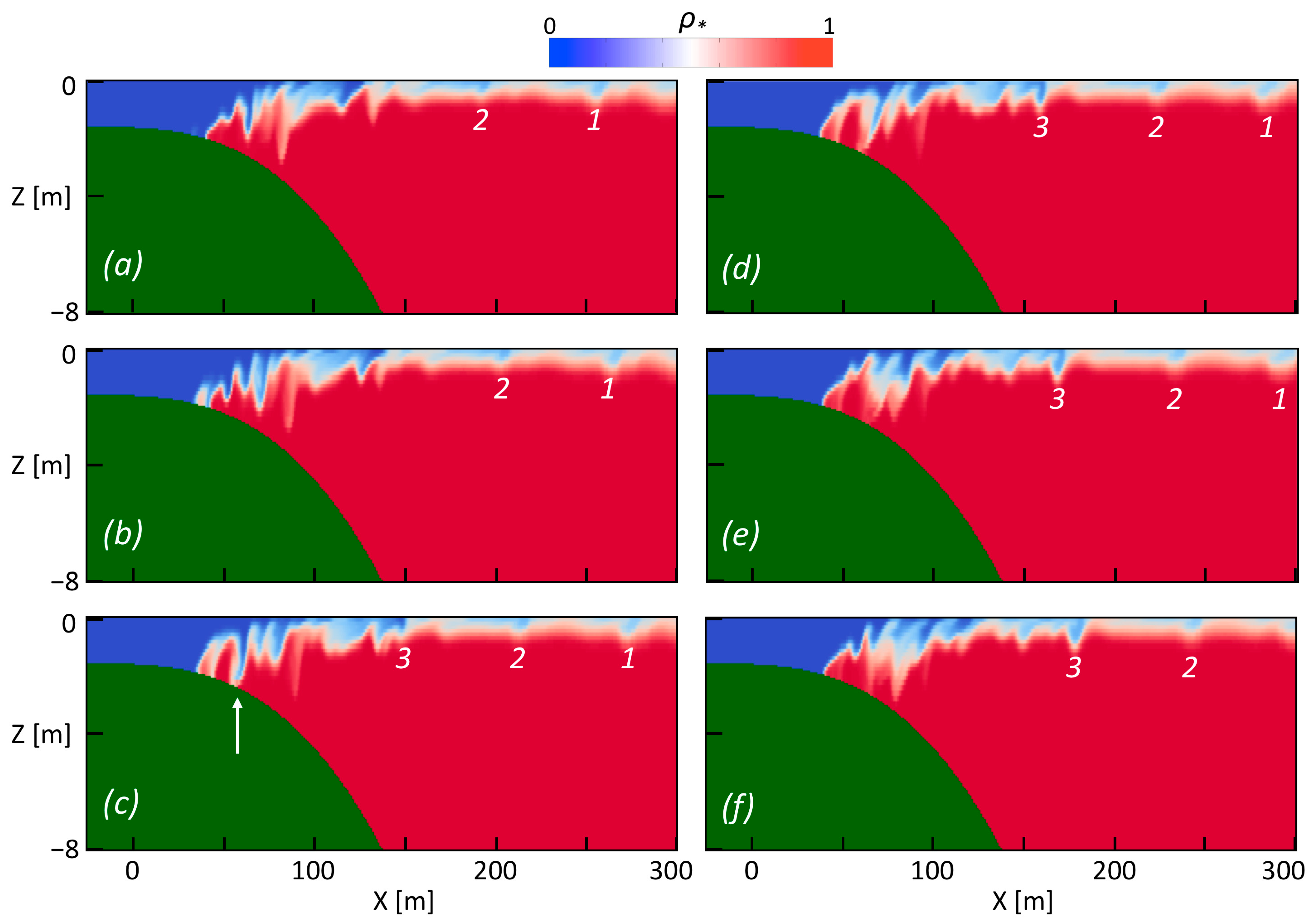
Viewed in a centerline vertical plane (Figure 6), the plume can be seen to lift off the bottom at x~40 m, then to develop shear instabilities, as expected from Figure 3e. The instabilities, which have horizontal wavelengths in the range of 10 to 12 m, result in vertical oscillations of the plume interface that are highly variable in both space and time (c.f., Figure 3c). In particular, localized penetrations of plume water to very near the seabed occur (Figure 6c, arrow) that are qualitatively similar to Osadchiev’s tow-yo data (Section 2.1). Beyond this region, from x~150 m, there emerge periodically localized downward bulges in the plume layer (Figure 6, features 1–3); these are incipient ring features.
3.3. Sensitivity to Inflow Speed and Geometry
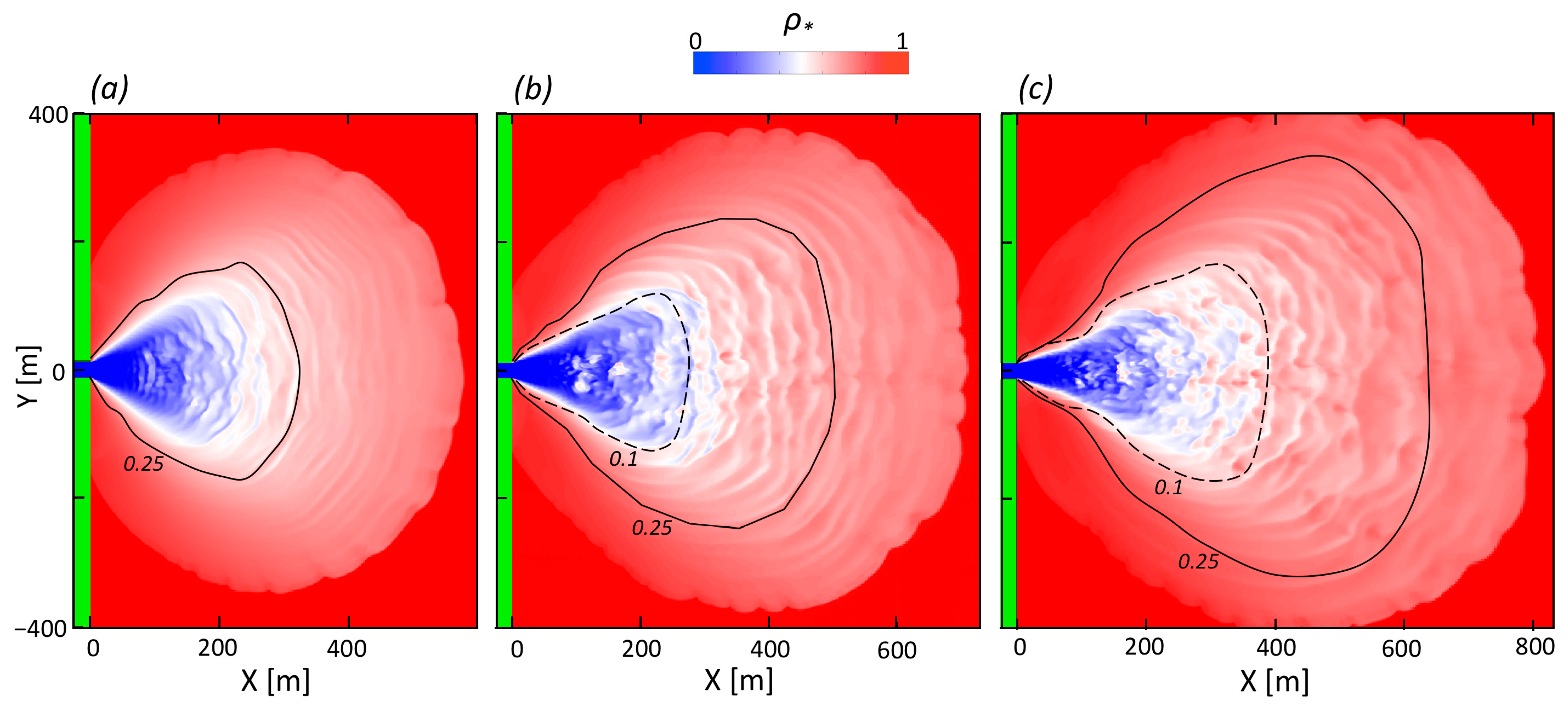
Sensitivity of the ring features to the model inflow velocity U0 is illustrated in Figure 7, for U0 values of 1, 1.5, and 2 m s−1. Compared with the base case (middle panel), rings appear more disorganized for larger inflow (right); but for smaller inflow (left) ring features emerge from the source region having an increased level of azimuthal coherence, and thus more closely resembling the real plume (Figure 1). This behavior is likely the consequence of higher levels of shear-induced turbulence with increasing U0; and is consistent with the increasingly larger areas of especially low Ri values (<0.1), as the lower the value of Ri is below its critical value of 0.25, the higher is the growth rate of KHI. Also increasing with inflow speed are the spacing of rings and their period (that is, time between creation of successive rings): the ring spacings are 29 ± 6 m, 37 ± 9 m, 39 ± 9 m, while their periods are about 45, 60, and 70 s. An explanation for those values eludes us. Additional cases (not shown) were done for still lower and higher inflow speeds. For U0 = 0.5 m s−1, or a discharge rate of only 21 m3 s−1, there are no rings at all; for U0 = 2.5 m s−1, which at 104 m3 s−1 is near the upper limit of the Mzymta discharge rate, the plume is further elongated, more generally turbulent, and without coherent rings. The model thus produces rings only over a middle range of discharge rates. This is qualitatively consistent with the real Mzymta River plume, as ring-like patterns are not apparent if the discharge rate is too low (less than about 50 m3 s−1), and often absent when the discharge rate is too high [4].
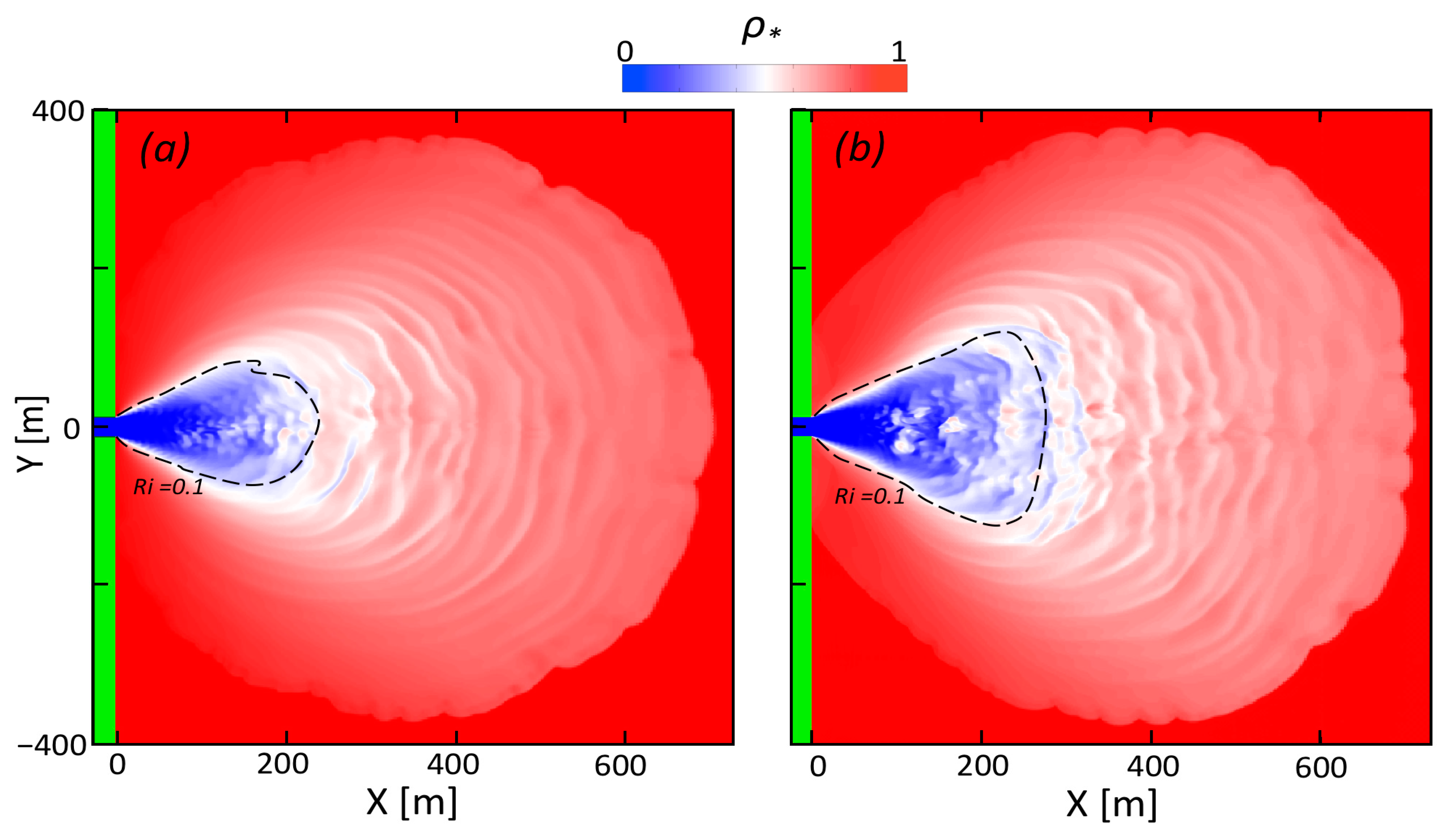
Runs were also done using different eddy-viscosity models, different model grids, and different river geometries and nearshore bathymetry. All these runs produced rings for U0 = 1.5 m s−1. An example, in which a flat ocean bottom was used, is shown in Figure 8a. In this case, the lift-off of the plume occurs uniformly across the width of the inflow, at x = 0; similar to a spreading, supercritical (Fri = 2.1) plume used in laboratory studies [2]. As compared with the sloping bathymetry result (Figure 8b), the area with very low values of Richardson number (Ri < 0.1) is reduced, indicating a reduction in the initial level of turbulence, and ring features emerge from the source region having an increased level of azimuthal coherence.
Overall model results suggest the physical mechanism responsible for creating rings is linked to spatially developing shear instabilities, arising after the point of lift-off. Development of KHI in an area of the plume where Ri ~ 0.1 appears to be consistent with the laboratory study by Yuan and Horner-Devine [2]. They found that the vorticity associated with KHI becomes aggregated into larger-scale structures, which stretch and maintain coherent shapes as the plume spreads laterally; but different from the model results, the laboratory structures were linear in shape, advanced more slowly than the plume front, and were observed only far behind the plume front. Just how coherent structures emerge from a turbulent low-Ri source region in the model plume is not clear; but a close examination of model animations does reveal behaviors that are not reported in the low-Reynolds-number laboratory study. These include pairing of KH instabilities, as well as a joining up, or merging, of initial ring fragments, both effects tending to increase length scales with increasing radial distance. Such effects, including their sensitivity to the model parameterization of turbulence, will need to be investigated further.
4. Conclusions
This study has attempted to achieve a clearer understanding of patterns of concentric rings occurring within small buoyant river plumes, as has been revealed recently in ocean color satellite imagery. The Mzymta River is used as a prototype for numerical simulations of the plume dynamics. The focus is on the near field of the plume, which is characterized by supercritical flow and enhanced mixing of the plume with ambient waters. The main result is that the model is able to produce ring-like features resembling those in the Mzymta plume. The rings are material features that, as compared with the bulk plume water, are deeper, more buoyant, and have more forward momentum. In the model, the origin of the rings appears linked to shear instability occurring close to the inflow source, which is as suggested by some previous work [2]. This is distinctly different from the internal wave hypothesis proposed in references [4,5,7,8]. Determining which dynamical viewpoint is closer to the truth will require additional study. A modeling issue is the sensitivity of the ring features to the mixing scheme parameterization. In the field, an experiment to test whether a ring is a material feature or a propagating one might be done by using a boat, or perhaps an aerial drone, to inject a fluorescent water-tracing dye into part of a ring, thus creating an artificial ocean color signal [21]. The subsequent spatial and temporal evolution of the dye can then be captured in an aerial survey [8]. If the dye and (turbid) ring move together—similar to our Figure 4—then rings are material features; if the ring propagates away from the dye, then rings are internal waves. Use might also be made of a horizontal acoustic Doppler current profiler, deployed either from a boat [22] to measure the radial motion of turbid rings through the plume, or from a near-shore station [23] to examine velocity structure within the lift-off and source regions.
Supplementary Materials
The following are available online at https://0-www-mdpi-com.brum.beds.ac.uk/article/10.3390/rs13071361/s1, Figure S1 (Video S1): Animation of surface density field, including particle tracking as in Figure 4.
Author Contributions
G.M. conceived the idea for this study and drafted the manuscript. T.E. did all the numerical work. All authors have read and agreed to the published version of the manuscript.
Funding
This work was supported by the Office of Naval Research under Naval Research Laboratory (NRL) Project 72-1R25-Z-0-5.
Institutional Review Board Statement
Not applicable.
Informed Consent Statement
Not applicable.
Data Availability Statement
No new data were created or analyzed in this study. Data sharing is not applicable to this article.
Acknowledgments
This is contribution NRL/JA/7230-20-0767.
Conflicts of Interest
The authors declare no conflict of interest.
References
- Horner-Devine, A.R.; Hetland, R.D.; MacDonald, D.G. Mixing and transport in coastal river plumes. Ann. Rev. Fluid Mech. 2015, 47, 569–594. [Google Scholar] [CrossRef]
- Yuan, Y.; Horner-Devine, A.R. Experimental investigation of large-scale vortices in a freely spreading gravity current. Phys. Fluids 2017, 29, 106603. [Google Scholar] [CrossRef]
- Garvine, R.W. Radial spreading of buoyant, surface plumes in coastal waters. J. Geophys. Res. Oceans. 1984, 89, 1989–1996. [Google Scholar] [CrossRef]
- Osadchiev, A.A. Small mountainous rivers generate high-frequency internal waves in coastal ocean. Sci. Rep. 2018, 8, 16609. [Google Scholar] [CrossRef] [PubMed]
- Osadchiev, A.A.; Zavialov, P.O. Structure and Dynamics of Plumes Generated by Small Rivers. In Estuaries and Coastal Zones—Dynamics and Response to Environmental Changes; Pan, J., Ed.; IntechOpen: London, UK, 2019. [Google Scholar]
- Marmorino, G.; Savelyev, I.; Smith, G.B. Surface thermal structure in a shallow-water, vertical discharge from a coastal power plant. Env. Fluid Mech. 2015, 15, 207–229. [Google Scholar] [CrossRef]
- Marchevsky, I.K.; Osadchiev, A.A.; Popov, A.Y. Numerical Modelling of High-frequency Internal Waves Generated by River Discharge in Coastal Ocean. In GISTAM; 2019; pp. 384–387. Available online: https://www.scitepress.org/Papers/2019/78402/78402.pdf (accessed on 1 December 2020).
- Osadchiev, A.; Barymova, A.; Sedakov, R.; Zhiba, R.; Dbar, R. Spatial Structure, Short-temporal Variability, and Dynamical Features of Small River Plumes as Observed by Aerial Drones: Case Study of the Kodor and Bzyp River Plumes. Remote Sens. 2020, 12, 3079. [Google Scholar] [CrossRef]
- Kilcher, L.F.; Nash, J.D. Structure and dynamics of the Columbia River tidal plume front. J. Geophys. Res. 2010, 115, C05S90. [Google Scholar] [CrossRef] [Green Version]
- Wang, C.; Wang, X.; Da Silva, J.C. Studies of internal waves in the strait of Georgia based on remote sensing images. Remote Sens. 2019, 11, 96. [Google Scholar] [CrossRef] [Green Version]
- Mendes, R.; da Silva, J.C.B.; Magalhaes, J.M.; St-Denis, B.; Bourgault, D.; Pinto, J.; Dias, J.M. On the generation of internal waves by river plumes in subcritical initial conditions. Sci. Rep. 2021, 11, 1–12. [Google Scholar] [CrossRef] [PubMed]
- Osadchiev, A.A.; Sedakov, R.O. Spreading dynamics of small river plumes on the northeastern coast of the Black Sea observed by Landsat 8 and Sentinel-2. Remote Sens. Environ. 2019, 221, 522–533. [Google Scholar] [CrossRef]
- Horner-Devine, A.R.; Chickadel, C.C. Lobe-cleft instability in the buoyant gravity current generated by estuarine outflow. Geophys. Res. Lett. 2017, 44, 5001–5007. [Google Scholar] [CrossRef]
- Horner-Devine, A.; Chickadel, C.C.; MacDonald, D. Coherent Structures and Mixing at a River Plume Front. In Coherent Flow Structures in Geophysical Flows at the Earth’s Surface; Venditti, J., Best, J.L., Church, M., Hardy, R.J., Eds.; Wiley: Chichester, UK, 2013; pp. 359–369. [Google Scholar]
- Marmorino, G.O.; Trump, C.L. Gravity current structure of the Chesapeake Bay outflow plume. J. Geophys. Res. 2000, 105, 28847–28861. [Google Scholar] [CrossRef]
- Delandmeter, P.; Lambrechts, J.; Marmorino, G.O.; Legat, V.; Wolanski, E.; Remacle, J.F.; Chen, W.; Deleersnijder, E. Submesoscale tidal eddies in the wake of coral islands and reefs: Satellite data and numerical modelling. Ocean Dyn. 2017, 67, 897–913. [Google Scholar] [CrossRef]
- Osadchiev, A.A.; Zavialov, P.O. Lagrangian model of a surface-advected river plume. Cont. Shelf Res. 2013, 58, 96–106. [Google Scholar] [CrossRef]
- OpenFOAM and The OpenFOAM Foundation. Available online: https://openfoam.org/ (accessed on 10 December 2020).
- Osadchiev, A. A method for quantifying freshwater discharge rates from satellite observations and Lagrangian numerical modeling of river plumes. Environ. Res. Lett. 2015, 10, 085009. [Google Scholar] [CrossRef] [Green Version]
- Osadchiev, A.; Korshenko, E. Small river plumes off the northeastern coast of the Black Sea under average climatic and flooding discharge conditions. Ocean Sci. 2017, 13, 465–482. [Google Scholar] [CrossRef] [Green Version]
- Savelyev, I.; Miller, W.D.; Sletten, M.; Smith, G.B.; Savidge, D.K.; Frick, G.; Menk, S.; Moore, T.; De Paolo, T.; Terrill, E.J.; et al. Airborne remote sensing of the upper ocean turbulence during CASPER-East. Remote Sens. 2018, 10, 1224. [Google Scholar] [CrossRef] [Green Version]
- Trump, C.L.; Allan, N.; Marmorino, G.O. Side-looking ADCP and Doppler radar measurements across a coastal front. IEEE J. Ocean Eng. 2000, 25, 423–429. [Google Scholar] [CrossRef]
- Marmorino, G.O.; Trump, C.L. Shore-based acoustic Doppler measurement of near-surface currents across a small embayment. J. Coast. Res. 2000, 16, 864–869. [Google Scholar]
Figure 1.
WorldView-3 image of the Mzymta River plume on 4 April 2017, illustrating the nearly concentric bands, or “rings”, that are the focus of this study. Shown are band 3 data (518 to 586 nm wavelengths), geo-referenced to a UTM map projection (zone 37N; WGS-84), and using square 1.4-m pixels. An independent color-composite version appears in reference [4]. WorldView-3 is a commercial Earth observation satellite owned by DigitalGlobe, Inc., Westminster, CO, USA.

Figure 2.
Model geometry. (a) Plan (x-y) view, showing spatial variation in horizontal resolution (∆x, ∆y). A 25 × 26-m notch in the shoreline represents the river inflow. (b) Vertical (x-z) section, showing offshore bathymetry; red lines indicate vertical resolution, which varies from 0.13 m near the surface to 0.46 m at the bottom.

Figure 3.
Representative model results, shown at t = 1630 s. (a) surface normalized density, 𝜌⁎; (b) surface velocity magnitude, |U|; (c) plume depth h, defined as where the normalized density 𝜌⁎ = 0.9; (d) Froude number, Fr; (e) Richardson number, Ri; (f) kinetic energy dissipation rate 𝜖, averaged over plume depth h; discontinuities in 𝜖 occur at jumps in the model grid spacing.

Figure 4.
Advection of surface water particles (black dots) chosen to lie initially within a ring feature. (a) Initial density field, t = 1280 s; (b) 7.7-min later, t = 1740 s. The ten initial particle positions were determined from local density minima within a specified subset area; subsequent particle positions were determined by computing their Lagrangian displacements, using the evolving surface velocity field at each model time step (∆t ~ 0.14 s). For clarity, the particles are shown larger than the underlying model cell dimension. An animation (Figure S1) shows particle positions every 10 s over the time period of (a) to (b).

Figure 5.
A Hovmöller (x-t) diagram showing the evolving centerline surface density. Rings, indicated by blue-white streaks, move at 1 m s−1 near their source region, but slow with increasing offshore distance. The plume front propagates into ambient water (red area) at a steady radial speed of 0.27 m s−1. The time period shown matches that in Figure S1.

Figure 6.
Centerline (x-z) section of normalized density, shown at 10-s intervals: (a) t = 1610 s; (b) t = 1620 s; (c) t = 1630 s; (d) t = 1640 s; (e) t = 1650 s; (f) t = 1660 s. Note that only the plume’s inner portion (x < 300 m) is being shown. Features 1–3 correspond to evolving ring features. Arrow in panel c points to a localized, near-bottom penetration of plume water.

Figure 7.
Variation of plume morphology with inflow velocity U0. (a) U0 = 1.0 m s−1; (b) U0 = 1.5 m s−1; (c) U0 = 2.0 m s−1. Corresponding values of river discharge rate are 42, 62, and 83 m3 s−1; values of inlet Froude number are 2.0, 2.9, and 3.9. Curves indicate values of Richardson number of 0.1 and 0.25; panel (a) has no 0.1 or lower values. Model time is 1630 s for each case.

Figure 8.
Variation of plume morphology with nearshore bathymetry: (a) flat ocean bottom; and (b) base case with nearshore slope. Curves indicate values of Richardson number of 0.1. Model time is 1630 s for each case.
Figure 8.
Variation of plume morphology with nearshore bathymetry: (a) flat ocean bottom; and (b) base case with nearshore slope. Curves indicate values of Richardson number of 0.1. Model time is 1630 s for each case.

Publisher’s Note: MDPI stays neutral with regard to jurisdictional claims in published maps and institutional affiliations. |
© 2021 by the authors. Licensee MDPI, Basel, Switzerland. This article is an open access article distributed under the terms and conditions of the Creative Commons Attribution (CC BY) license (https://creativecommons.org/licenses/by/4.0/).
Share and Cite
MDPI and ACS Style
Marmorino, G.; Evans, T. Interpreting Patterns of Concentric Rings within Small Buoyant River Plumes. Remote Sens. 2021, 13, 1361. https://0-doi-org.brum.beds.ac.uk/10.3390/rs13071361
AMA Style
Marmorino G, Evans T. Interpreting Patterns of Concentric Rings within Small Buoyant River Plumes. Remote Sensing. 2021; 13(7):1361. https://0-doi-org.brum.beds.ac.uk/10.3390/rs13071361
Chicago/Turabian StyleMarmorino, George, and Thomas Evans. 2021. "Interpreting Patterns of Concentric Rings within Small Buoyant River Plumes" Remote Sensing 13, no. 7: 1361. https://0-doi-org.brum.beds.ac.uk/10.3390/rs13071361
Note that from the first issue of 2016, this journal uses article numbers instead of page numbers. See further details here.