
Deep Metric Learning with Online Hard Mining for Hyperspectral Classification


1
Hubei Subsurface Multi-Scale Imaging Key Laboratory, Institute of Geophysics and Geomatics, China University of Geosciences, Wuhan 430074, China
2
Key Laboratory of Intelligent Computing & Signal Processing, Ministry of Education, Anhui University, Hefei 230601, China
*
Author to whom correspondence should be addressed.
Remote Sens. 2021, 13(7), 1368; https://0-doi-org.brum.beds.ac.uk/10.3390/rs13071368
Submission received: 14 March 2021
/
Accepted: 30 March 2021
/
Published: 2 April 2021
(This article belongs to the Special Issue Explainable Deep Neural Networks for Remote Sensing Image Understanding)
Abstract
:Recently, deep learning has developed rapidly, while it has also been quite successfully applied in the field of hyperspectral classification. Generally, training the parameters of a deep neural network to the best is the core step of a deep learning-based method, which usually requires a large number of labeled samples. However, in remote sensing analysis tasks, we only have limited labeled data because of the high cost of their collection. Therefore, in this paper, we propose a deep metric learning with online hard mining (DMLOHM) method for hyperspectral classification, which can maximize the inter-class distance and minimize the intra-class distance, utilizing a convolutional neural network (CNN) as an embedded network. First of all, we utilized the triplet network to learn better representations of raw data so that raw data were capable of having their dimensionality reduced. Afterward, an online hard mining method was used to mine the most valuable information from the limited hyperspectral data. To verify the performance of the proposed DMLOHM, we utilized three well-known hyperspectral datasets: Salinas Scene, Pavia University, and HyRANK for verification. Compared with CNN and DMLTN, the experimental results showed that the proposed method improved the classification accuracy from 0.13% to 4.03% with 85 labeled samples per class.

1. Introduction
With the exponential development of hyperspectral remote sensing imaging technology, hyperspectral imaging spectrometers can capture high spatial resolution images with hundreds of narrow spectral bands. Meanwhile, hyperspectral remote sensing images have abundant spectral and structural information for the analysis and detection of features. As a result, hyperspectral images have been utilized for a wide variety of applications, such as precision agriculture [1], environmental monitoring [2], and mineral exploration [3,4]. Among these applications, one of the most attractive fields in the research of hyperspectral images is hyperspectral classification.
There have a lot of different hyperspectral classification algorithms being proposed. Depending on whether a priori knowledge is used or not, the popular hyperspectral classification algorithms comprise an unsupervised and supervised classification [5]. Unsupervised learning, in the absence of a given prior knowledge, automatically classifies or clusters the input data to find the model and law of the data. The more representative unsupervised algorithms are principal component analysis [6], locally linear embedding [7], and independent component analysis [8], which utilize the selected prominent features to reduce the dimensionality of original data. However, the classification accuracy of unsupervised algorithms is not as high as that of supervised classification algorithms. Supervised approaches utilize a group of training samples to classify input data for each category, such as maximum likelihood methods, support vector machine [9], sparse/spatial nonnegative matrix underapproximation [10], neural networks [11], and kernel-based methods [12,13,14]. For instance, Li et al. [15] proposed a generalized framework for composite kernel to flexibly balance spatial, spectral information, and computational efficiency. Although hyperspectral classification is widely studied, there are still two problems: (1) hundreds of narrow spectral bands leading to the “curse of dimensionality”, and (2) limited labeled samples for training.
To further handle the Hughes phenomenon [16] (when the number of training samples is limited, the performance of classification decreases as the feature dimension increases), researchers have extensively studied deep learning-based methods. The feature dimension refers to the number of features in the feature space. Deep learning is a hierarchical structure of deep neural networks, usually more than three layers deep. The hierarchical structure attempts to extract the deep features of the input data on a hierarchical basis. Deep learning is a rapidly developing research field that has shown usefulness in many research fields, such as computer vision and pattern recognition [17,18]. In the field of hyperspectral classification, there have been proposed many deep models. Yuan et al. [19] proposed a stacked auto-encoder (SAE) model for hyperspectral classification, where SAE was employed to obtain valuable advanced features. Since then, an increasing number of deep learning models have been proposed, such as deep belief network [20], recurrent neural network (RNN) [21], and convolutional neural network (CNN) [22,23,24]. Although methods based on deep learning have made great strides in dimensional reduction of the hyperspectral image, they all need numerous labeled samples to train many parameters, which is known in deep learning as the small sample set classification problem. Many strategies have been used to better tackle such problems. For instance, Li et al. [25] proved that by constructing pixel-pair samples, the number of training samples will increase significantly. More recently, a multi-grained network has been proposed as a hyperspectral classification method based on deep learning, with the aim of classifying hyperspectral data on a small scale [26]. Wu et al. [27] proposed a semi-supervised deep learning framework whereby large amounts of unlabeled data, with their pseudo labels, were used to pretrain a deep convolutional recurrent neural network, and then refine the network with the limited labeled data available.
In this paper, a model with online hard mining based on deep metric learning (DMLOHM) has been proposed, which is a powerful deep embedded model for extracting features and classifying pixel-level hyperspectral remote sensing images. The first thing to do is to obtain embedded feature space by feeding all samples into the embedded network separately. Secondly, a random hardest negative sampling strategy is utilized to select the hardest triplets from the embedded feature space, which ensures that all triplets are valid. Finally, to obtain the optimal parameters of the model, we used all the hardest triplets to train a deep metric learning-based model. The objective of the proposed model is to project the hyperspectral input features into Euclidian space where the mapping features have a minimum intra-class distance and a maximum inter-class distance. The online hard mining strategy is used to seek valid triplets (a triplet is composed of an anchor, a positive sample of the same class as the anchor, and a negative sample of the different class as the anchor) from mapping features while improving operational efficiency. In comparison to other related advanced methods, our proposed methodology comprises three key contributions, which are summarized below.
- (1)
- A model based on deep metric learning is proposed for hyperspectral classification. By utilizing the ability of the deep metric learning-based approach to maximize distances between classes and minimize distances within classes, one can effectively reduce the high dimensionality of hyperspectral data while achieving a high classification accuracy.
- (2)
- We introduce the idea of online hard mining for deep metric learning to mine the most discriminative triplets while improving the performance of triplet network. Triplets obtained through an online hard mining strategy are more effective with limited labeled data, significantly improving the classification accuracy.
- (3)
- The experimental results show that the proposed method is superior to other comparison methods for comparing multiple hyperspectral image datasets.
The remaining sections of this paper are constructed as follows. Section 2 presents the background of relevant research. Section 3 provides detailed information about the proposed deep metric learning-based model. Section 4 presents the experimental results of the proposed methodology using three actual hyperspectral datasets. Finally, the conclusions are described in Section 5.
2. Related Work
In our proposed approach, convolutional neural networks are used as an embedded network of the deep metric learning model. As a result, the fundamental structure of convolutional neural networks is first presented here. Next, we present the research related to deep metric learning and sample mining strategy.
2.1. Convolutional Neural Network
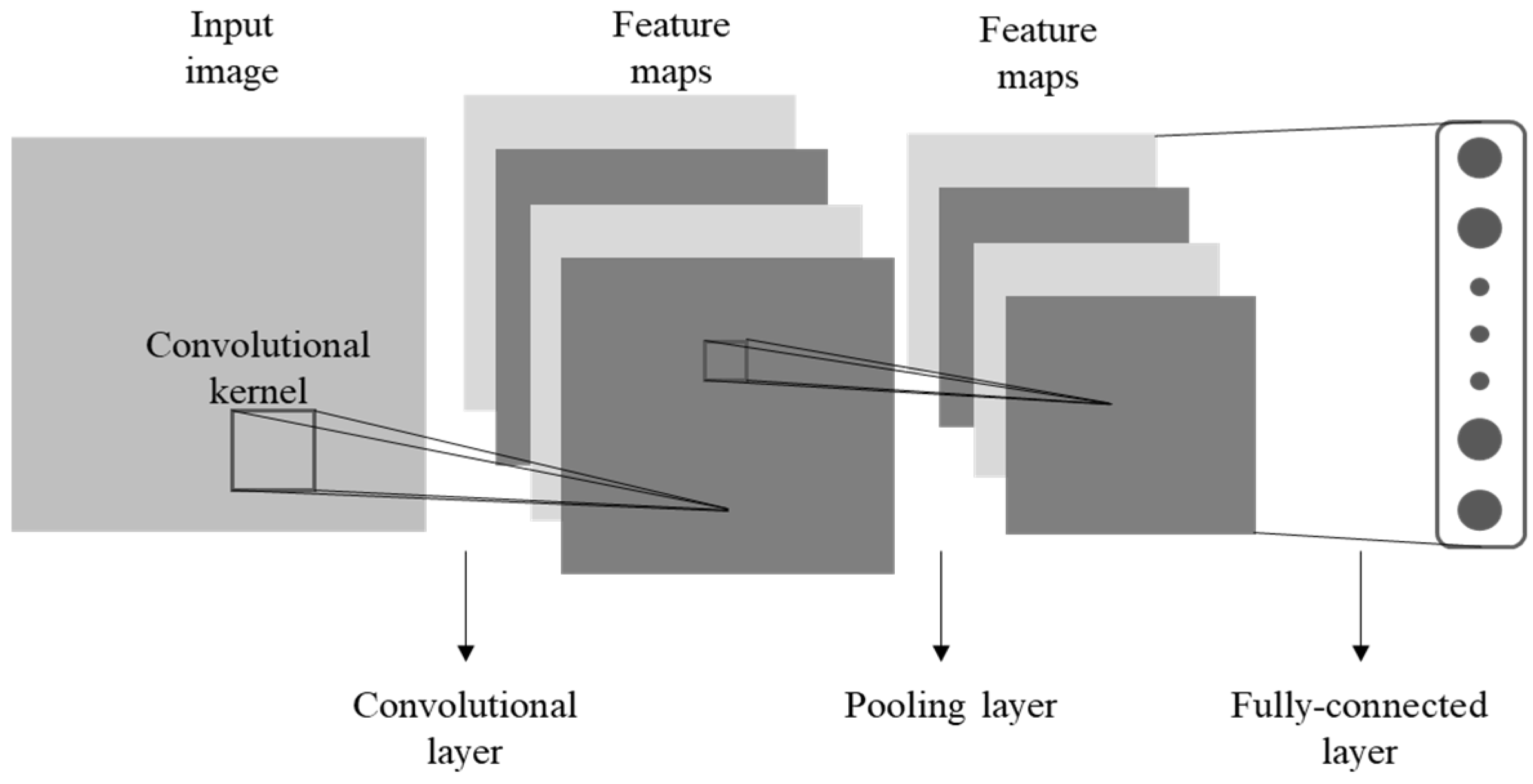
In recent times, CNN has achieved outstanding achievements in a wide range of applications, notably the analysis of images by remote sensing [28,29,30]. Therefore, CNN [22], which is stress-free handling of high-dimensional data, is used as an embedded network for our proposed model on the basis of deep metric learning. As Figure 1 shows, the fundamental structure of a CNN is constructed as a set of layers, consisting of convolutional layer, pooling layer, and fully connected layer.
2.1.1. Convolutional Layer
These are particularly important in the extraction of feature. The first convolutional layer typically obtains low-level features, while the high-level features can be extracted from the deeper convolutional layers by combining low-level features. In a convolutional layer, the connection between each neuron and the local patch in the feature map of the previous layer is by means of a group of convolutional kernels. Next, the result of this locally weighted sum passes by a nonlinearity operation, such as a hyperbolic function (tanh) and rectified linear unit (ReLU). In a feature map, all neurons share the same convolutional kernels. At the meantime, different feature maps commonly utilize different convolutional kernels in the convolutional layer. Thus, the output volume generated by the layer is calculated as , where is the convolutional kernel of layer , is the output volume of layer , and the bias matrix of the layer is .
2.1.2. Pooling Layer
In general, there is a pooling layer after each convolutional layer, which is created by the calculation of some local non-linear operations on a small spatial region of the feature map. Reducing the dimension of the representation and establishing invariants for small translations or rotations is the objective of the pooling layer [30]. A commonly used pooling operation is the max-pooling operation that calculates the maximum of a local patch of units into a single feature map. The pooling results of the layer is calculated as .
2.1.3. Fully Connected Layer
The last few layers of a convolutional neural network are usually fully connected layers, which helps to better aggregate the information conveyed at lower levels and to make final decisions.
2.2. Deep Metric Learning
Learning a self-defined distance metric that can be utilized to calculate the similarity between two samples is the goal of metric learning. For instance, Wang et al. [31] utilized a locality constraint to assure the local smoothness and preserve correlation between samples for traffic congestion detection. According to Weinberger and Saul [32], an appropriate distance metric can significantly improve the performance of many visual classification tasks. Since Hinton et al. [20] introduced deep learning concept in 2006, more and more deep models have been increasingly proposed. The aim of deep models is to learn valuable semantic representations of data that can then be used to distinguish between available classes [33,34,35]. However, such representations and the corresponding induction measures are often considered to be side effects of the classification task, rather than being explicitly investigated [36]. Therefore, Hadsell et al. [37] proposed the Siamese network variants for distinguishing between similar pairs and dissimilar pairs of examples, in which a contrastive loss is utilized to train the network. As the concepts of similarity and dissimilarity require context, Siamese networks are also sensitive to calibration. A triplet network model was proposed by Hoffer et al. [36], aiming at learning valuable representations through a comparison of distances. Deng et al. [38] utilized a triplet network based on metric learning and the mean square error (MSE) loss to classify hyperspectral image data, which significantly improves the results of limited labeled samples classification. Although triplet network have been successfully implemented as a deep metric learning model to perform classification tasks using only a small amount of training data [38], the triplet generation method is not efficient, which needs to be improved. Our proposed approach, which guarantees valid information about the features, utilizes a hard negative mining strategy with an online method to generate triplets.
2.3. Sampling Mining Strategy
Informative input samples, the structure of the network model, and a metric loss function [39] together constitute the concept of deep metric learning. While the loss function is critical for deep metric learning, the selection of informative samples is also vital for the classification or clustering task. Sampling strategies can improve the success rate of the network and the speed at which the network can be trained. Earlier, a sampling strategy of a random selection of positive and negative sample pairs was adopted in the Siamese network [40]. For face sketch synthesis, Wang et al. [41] reduced the time consumption by utilizing an offline random sampling strategy, which shows strong scalability. However, Simo-Serra et al. [42] pointed out that the learning process may slow down and be adversely affected after the network has achieved a level of acceptable performance. To overcome this issue, it is highly effective to employ more realistic training models with a better sampling strategy, such as semi-hard negative mining and hard negative mining, while using informative samples. Semi-hard negative mining [43] focuses on finding negative samples in the margin. False-positive samples determined by training data correspond to hard negative samples [39]. When the anchor is too near to the negative samples, the variance of the gradient is high, and the signal-to-noise ratio of the gradient is low. Thus, Manmatha et al. [44] proposed a distance-weighted sampling strategy to filter out noisy samples.
In summary, although we can create a good network model and architecture, the network learning ability is still limited by the discriminatory ability of the samples that are presented to the network. Thus, differentiated training samples of each category should be submitted to construct the network, in order for the network to be able to learn better and to obtain a representation of the features.
3. Deep Metric Learning with Online Hard Mining
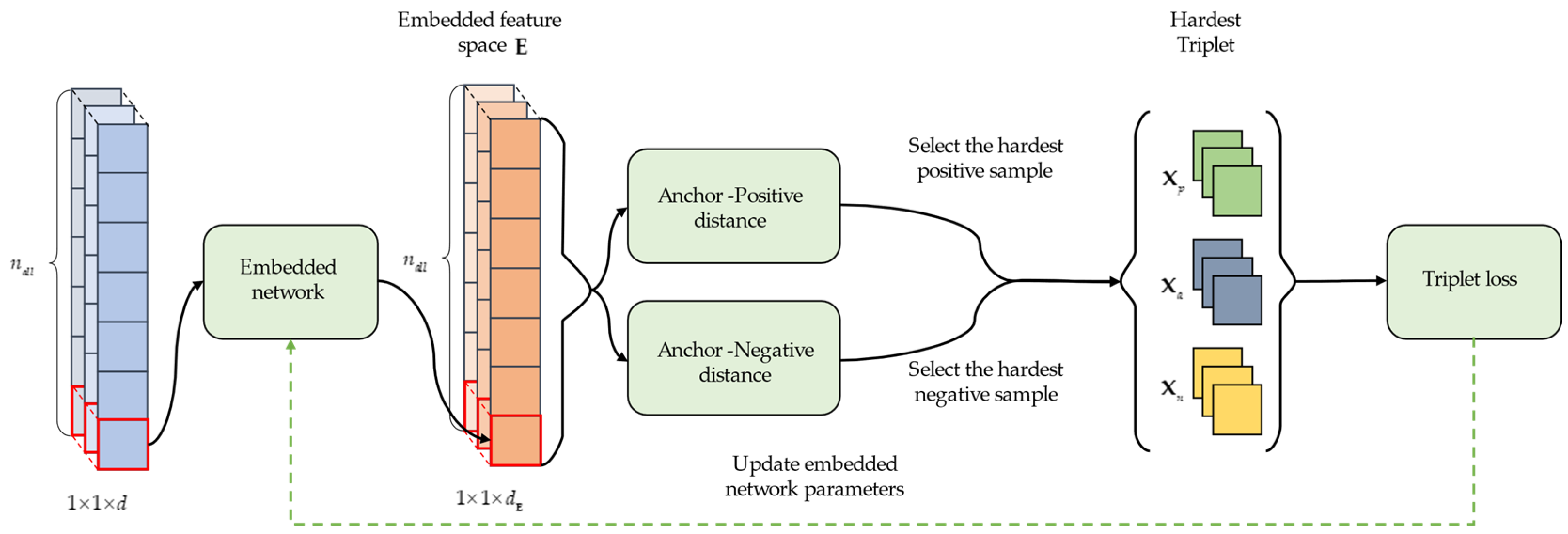
To tackle the challenge of the Hughes phenomenon and limited labeled samples in hyperspectral classification, we constructed a model based on deep metric learning that embeds samples into a specific metric space in which the distance between any two samples can be characterized. At first, all samples are individually fed into the embedded network mentioned in Section 2.1, rather than in triplet form, to obtain embedded feature space , which will reduce computational consumption. Secondly, the hardest triplets are selected from the embedded feature space by utilizing a random hardest negative sampling strategy, which ensures that all triplets are valid. Finally, the hardest triplets are used to train a deep metric learning-based model to obtain the optimal parameters of the model. Figure 2 shows the flowchart of our proposed method.
3.1. Deep Metric Learning-Based Model
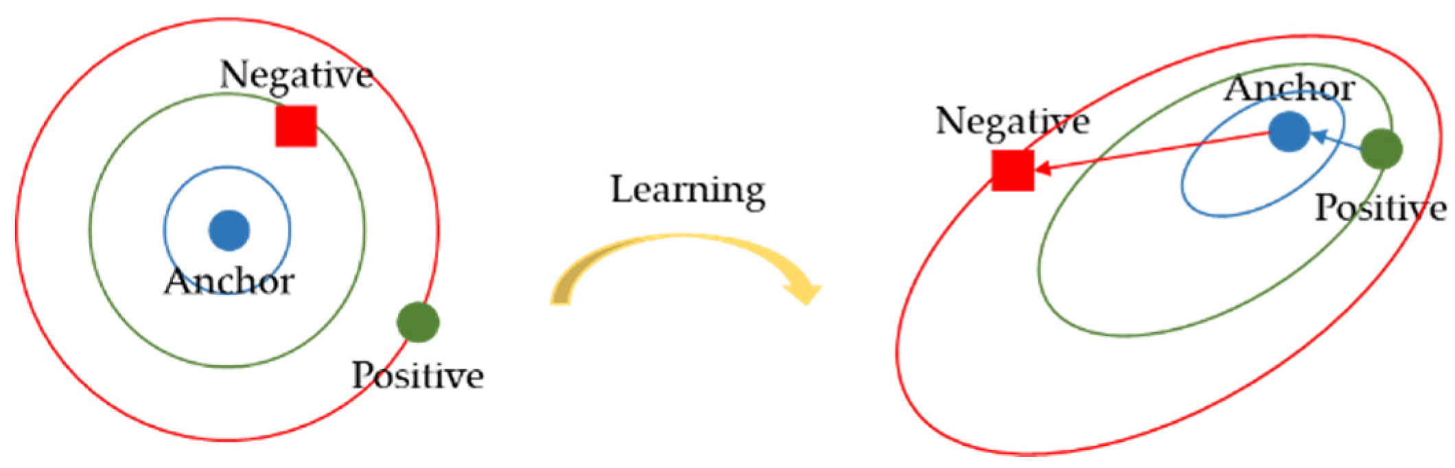
Three same feed-forward embedding network instances with shared parameters form a triplet network, which is a typical model in deep metric learning. The embedding network is represented by , which embeds a sample into a d dimensional Euclidean space . As a result, the input data form of the triplet network is , where to have the same class labels and have different class labels. The term is known as an anchor of a triplet. In a triplet network, it is important to calculate the distance between the positive sample, negative sample, and the anchor.
where represents the Euclidean distance between two samples. After calculating the distances between the anchor, positive, and negative samples, one can calculate the standard loss function of the triplet network [44] as
where is a margin, which is enforced between positive and negative pairs. Pulling the positive samples (green dot) closer to the anchor (blue dot) while pushing the negative samples (red square) far away is the objective of triplet loss. The blue arrow represents pulling in, and the red arrow represents pushing away, as shown in Figure 3.
3.2. Deep Metric Learning for Online Hard Mining
When training the triplet network mentioned above, one must often necessarily form triplets of anchor, positive samples, and negative samples at first, and then cast the triplet batches into triplet network to obtain the embedded features. Specifically, assuming that C (C is the number of generated triplets) triplets are generated in the manner described above, 3C convolutional neural network operations must be computed to obtain the triplets consisting of C embedded features. Then, the loss of these C triplets is calculated and finally backpropagated to the network. Generally, such a training procedure, which is known as an offline training strategy, is not efficient [43].
Therefore, Schroff et al. [43] proposed an online method for generating triplets. It is assumed that the C triplets are generated online. First, the embedded features of the C input samples are obtained by using a convolutional neural network, which is computed C times. Then, these C embedded features are used to generate triplets (up to a maximum of triplets). Compared to the traditional method of generating triplets, it appears that the online method of generating triplets reduces the number of operations by 2C times, but not all triplets generated by the online method is valid triplets. To overcome the problem of valid triplets, we combine the sampling strategy of Hermans et al. [45] with the online approach for generating triplets to form our deep metric learning with the online hard mining (DMLOHM) method, which can be seen in Algorithm 1. The core idea of valid triplets mining is to form batches by randomly sampling P (P is the total number of classes in all samples) classes, and then randomly sampling K (K is the number of samples by randomly sampling) samples of each class. Thus, the total number of samples in a batch is PK. For each sample in a batch, we can select the most challenging positive and negative samples in the batch. The final loss function of DMLOHM can be formulated as
where represents hinge function, if the value in the formula is less than , then is equal to ; otherwise, vice versa.
For DMLOHM, the online method and hard triplet mining is adopted for efficiently generating valid triplets. Moreover, generating valid triplets allows for the production of more discriminative information. With the help of valid triplets, it is now possible to perform hyperspectral classification without many training samples.
| Algorithm 1 A single iteration for training the DMLOHM |
| Input: Model: The training set , where Parameter: the value of margin m (set as 0.1) Output: Updated model |
| Begin 1. Obtain the embedded features through the embedded net. 2. Utilize the random hardest negative sampling strategy to get the hardest positive samples and hardest negative samples from the embedded features . 3. Calculate the distance of anchor-positive samples and the distance of anchor-negative samples by (1). 4. Calculate the loss by (3) with margin m. 5. Update parameter sets by backpropagating through . End |
4. Experiments and Analysis
Due to several critical problems, including the “curse of dimensionality” and limited labeled samples for training, we proposed a deep metric learning-based method to tackle these two problems. We used high-dimensional hyperspectral images to verify the former problem and used different sample sampling strategies to verify the latter problem. Firstly, to demonstrate the performance of the proposed DMLOHM algorithm, we implemented experiments on three publicly available datasets, which were commonly used in hyperspectral classification, namely, the Salinas dataset, the Pavia University dataset, and the HyRANK dataset [46,47]. These datasets are described in detail as follows. Then, a detailed analysis was made for the hyperparameters in the model.
4.1. Dataset Description
4.1.1. Salinas Dataset
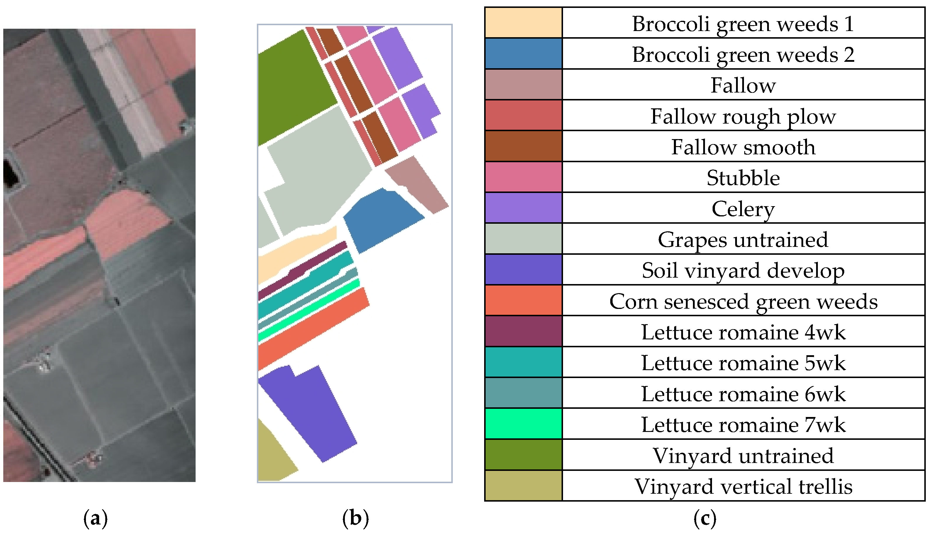
The Salinas dataset was acquired by the Airborne Visible/Infrared Imaging Spectrometer (AVIRIS) sensor over Salinas Valley, California, USA [38], which can be downloaded from http://www.ehu.eus/ccwintco/index.php (accessed on 30 March 2021). There are 204 spectral bands available after removing the 20 water absorption bands. The spatial size of this dataset was 512 × 217, with a spatial resolution of 3.7 m. The pseudo-color composite image and ground truth map of the Salinas dataset can be seen in Figure 4. There were 16 types of land cover with 54,129 labeled pixels in total, and the specific information is shown in Table 1.
4.1.2. Pavia University Dataset
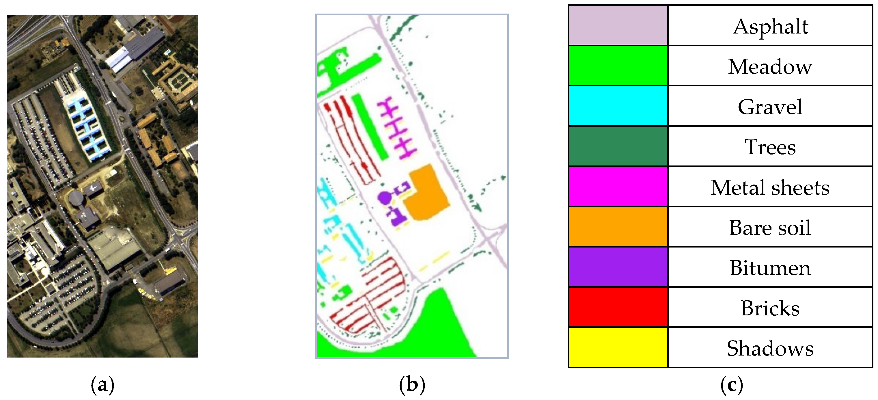
The Pavia University dataset was acquired by the Reflective Optics System Imaging Spectrometer (ROSIS) sensor during a flight campaign over Pavia, Northern Italy [48], which can be download from http://www.ehu.eus/ccwintco/index.php (accessed on 30 March 2021). After we removed 12 noisy bands, 103 spectral bands remained in the Pavia University dataset. The spectral range of bands was between 430 and 860 nm. The spatial resolution and spatial size were 1.3 m and 610 × 340, respectively. The pseudo-color composite image and ground truth map of the Pavia University dataset can be seen in Figure 5. As shown in Table 2, there were nine types of land cover with a total of 42,776 labeled pixels.
4.1.3. HyRANK Dataset
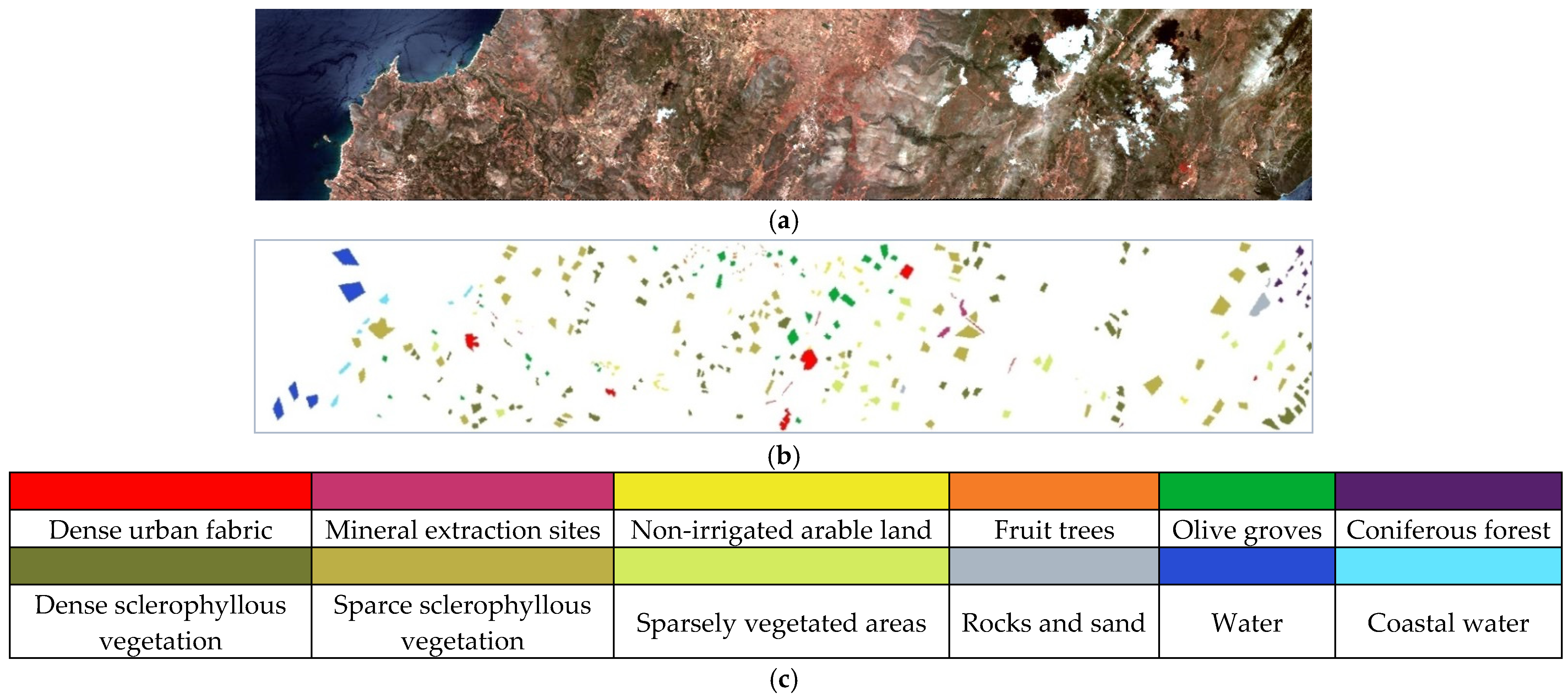
The HyRANK dataset was acquired by the Hyperion sensor on the Earth Observing-1 satellite with a spatial resolution of 30 m. It includes five images, two of which (i.e., Dioni and Loukia) can be used as training hyperspectral images and three of which (i.e., Erato, Kirki, and Nefeli) can be used as validation hyperspectral images. Since only the Dioni has a sample size greater than 100 in each category, Dioni was chosen as our experimental data. The spatial size of the HyRANK dataset was 250 × 1376, with 176 spectral bands, which can be downloaded from http://www2.isprs.org/commissions/comm3/wg4/ (accessed on 30 March 2021). The pseudo-color composite image and ground truth map of the Dioni dataset can be seen in Figure 6. As Table 3 shows, there were 12 types of land cover with total of 20,024 labeled pixels.
4.2. Experimental Setting
To illustrate the efficiency of the proposed method for reducing hyperspectral dimensionality and classifying limited labeled samples, we compared DMLOHM with four deep learning classification algorithms, i.e., auto-encoder (AE), recurrent neural network (RNN) [21], CNN [22], and deep metric learning with triplet network (DMLTN) [36]. Because of the single-pixel hyperspectral data as sequential data, we chose Hu’s 1-D (one dimensional) CNN [22] as the embedded network of DMLOHM and DMLTN. In this paper, overall accuracy (OA), average accuracy of each class (AA), and kappa coefficient (kappa) were the performance metrics. The OA score assesses the overall classification accuracy, i.e., the number of samples correctly classified in all categories divided by the total size of testing samples and the average of each classification accuracy per class is the AA score. Kappa is a statistical measure relating to the degree of agreement of categorical items [49,50].
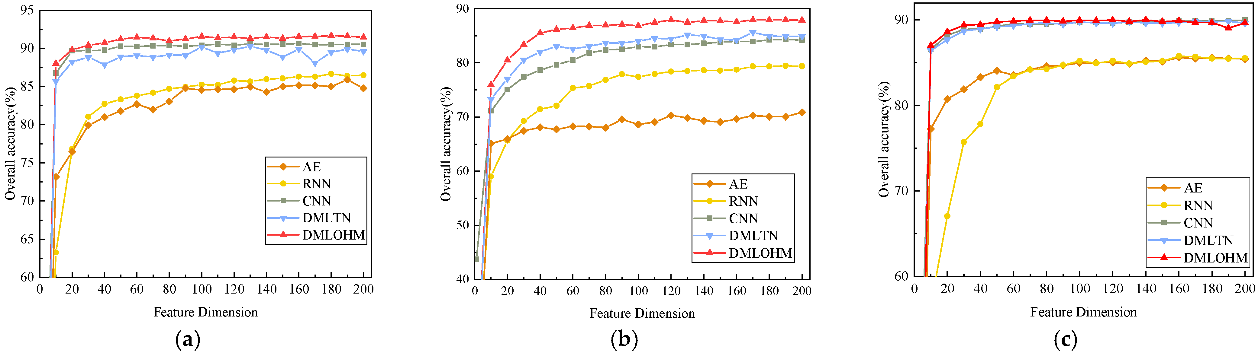
For the dimensionality reduction of the hyperspectral image, we performed the following experiments, setting extracted feature dimension to start at 1 dimension and then increment to 200 in 10 intervals, utilizing 85 samples per class as the training set. Since we were also interested in limited labeled samples classification, likewise, the experimental parameter setting was that randomly picking out a very few numbers of labeled samples per class (e.g., 10, 25, 40, 55, 70, 85, and 100) from the labeled set was to constitute the training set, and then the testing set consisted of the rest of the labeled samples. After considering the results of feature dimensions, we set the feature extraction dimension of the limited labeled sample classification to 128, which is abbreviated as Dim, in order to obtain stable and better classification results. Here, we took the average OA and kappa values of 10 experimental results as a measure of the performance of the different classification algorithms.
4.3. Parameter Setting and Convergence Analysis
As for training configuration, we ran our training procedures in a PyTorch environment with Adam optimization algorithm, and experiments were performed on Nvidia RTX2060 with memory usage limited to 6 GB. For the proposed model, the learning process was stopped after 200 training epochs without the validation set, and the learning rate was set as 0.001. The hyperparameter, margin value m, also affects the classification accuracy of DMLOHM. Thus, we performed an experimental analysis of this parameter, utilizing 85 samples per class as a training set while setting the feature extraction dimension as 128, and the result is shown in Figure 7a. From Figure 7a, we set the important margin value m as 1. As shown in Figure 7b, our DMLOHM approach converged smoothly in the training procedure.
5. Results
To tackle the “curse of dimensionality”, many academics have studied the ability of deep learning models to deal with this problem. Thus, in this paper, the dimensionality reduction effect of our proposed method was analyzed by comparing the classification accuracy of different algorithms from 1 to 200 dimensions. Experiments that compared the classification accuracy of various algorithms when sampling 10, 25, 40, 55, 70, 85, and 100 samples per class were also set up to analyze the ability of our proposed approach to deal with limited labeled samples classification problems.
5.1. Dimensionality Reduction
Figure 8a–c shows variation of classification OA values with differential extracted feature dimensions of Salinas dataset, Pavia University dataset, and HyRANK dataset, respectively. The dimension of the experiment was set to take one dimension as a single dimension, and then, starting with 10 dimensions, with 10 as an interval, until 200 dimensions were taken. The following separately analyzed the experimental results. For the Salinas dataset, when the feature dimension reached 10 dimensions, the classification accuracy of DMLOHM was comparable to that of CNN but much higher than those of AE, RNN, and DMLTN. For the Pavia University dataset, DMLOHM outperformed the other comparison algorithms when the feature dimension reached 10. DMLOHM achieved the best classification result of about 40 feature dimensions. Then, the classification accuracy of the DMLOHM algorithm gradually stabilized at a certain numerical range. For the HyRANK dataset, DMLOHM was able to achieve the best classification result when the number of feature dimensions reached 25, which was optimal earlier than any other algorithm.
What is obvious from Figure 8 is that the DMLOHM algorithm can effectively reduce the dimensions of hyperspectral data and improve the Hughes phenomenon. Meanwhile, our proposed method performed with better OA in most situations (when the feature dimension was greater than 10 dimensions).
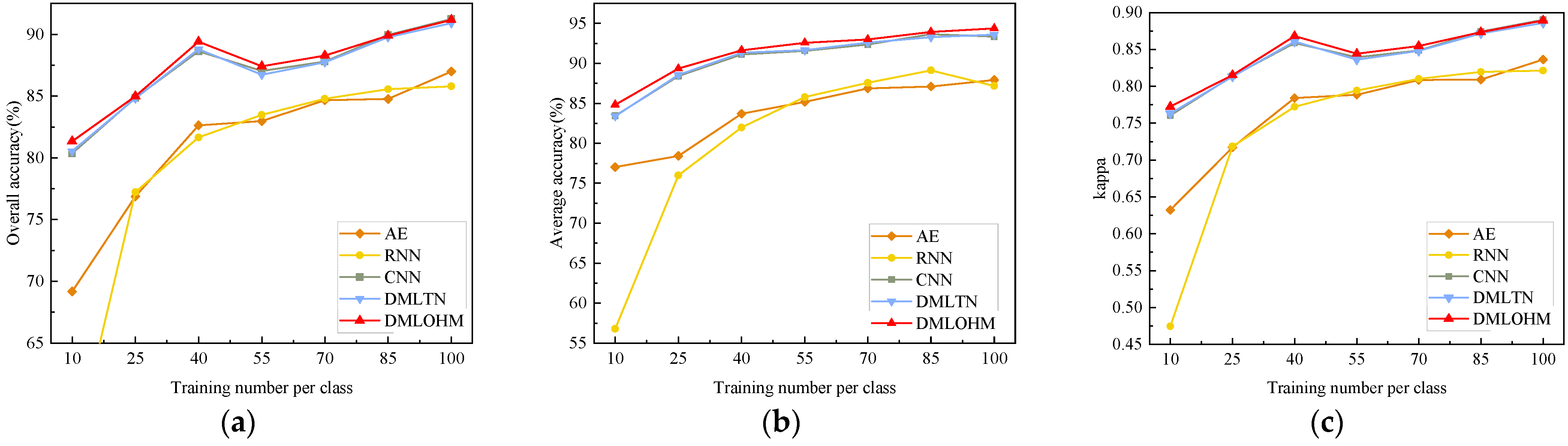
5.2. Limited Labeled Samples Classification
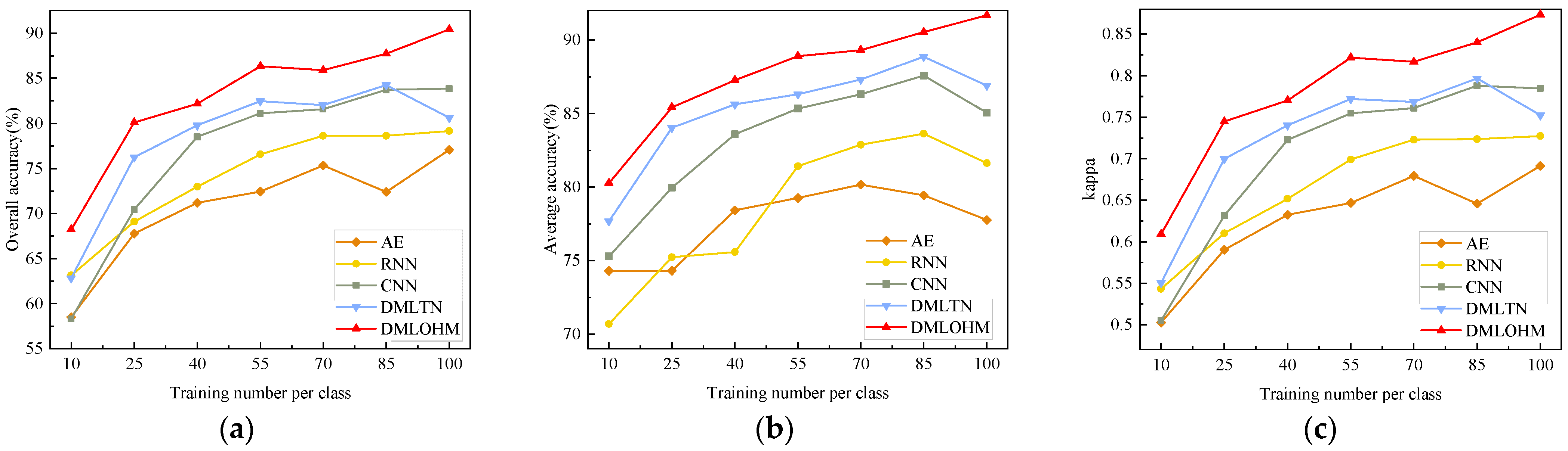
Figure 9, Figure 10 and Figure 11 show the classification accuracies of the Salinas dataset, Pavia University dataset, and HyRANK dataset, respectively, including OA, AA, and kappa of all comparison methodologies in three datasets with different numbers of training samples per class. The feature extraction dimension of all the comparison methods was set up to 128. For the Salinas dataset and Pavia University dataset, the classification accuracy of DMLOHM always outperformed other algorithms with limited labeled samples, especially the Pavia University dataset. For instance, in terms of the difference in classification accuracy between DMLOHM and DMLTN, CNN was greater when the number of samples was 10 per class than when the number of samples was 85 per class. As for the Pavia University dataset, we can see that our DMLOHM method outperformed the comparison algorithms with the highest classification accuracy and the best robustness. Compared to CNN, which was used as the embedded network of DMLOHM, DMLOHM improved the classification accuracy by about 9%. Likewise, compared to DMLTN, DMLOHM substantially outperformed DMLTN, especially when the training sample was 100 per class, which improved the classification accuracy by 7.72%. The superior performance of the DMLOHM approach was also reflected on the HyRANK dataset, which is shown in Figure 11. From 10 training samples per class to 100 training samples per class, the classification accuracy of DMLOHM has always been better than other algorithms. That is, DMLOHM algorithm can boost the classification accuracy with limited training samples.
From the results of limited labeled samples classification, when the number of samples was small, our proposed method was able to effectively improve the classification accuracy.
5.3. Other Experiments
Table 4, Table 5 and Table 6 summarize the quantitative evaluation results of the three datasets, with 85 labeled samples per class, while reducing the original dimension to 128 dimensions. The indicators for quantitative analysis of the results were classification accuracy of each class, the average accuracy, the average OA with the corresponding standard deviation, and the average kappa coefficient with standard deviation. Here, all the experiments were repeated 10 times. The best results for each indicator are labeled in bold.
As shown in Table 4, the proposed approach achieved the best classification accuracy in most individual classes and obtained the highest OA and kappa coefficient values for the Salinas dataset. It was observed that DMLOHM classified the vinyard untrained much better than the other algorithms and reached 78.20%, being 5.4% higher than DMLTN. Moreover, the classification accuracy of each class showed that DMLOHM presented a higher accuracy with a robust classifier performance because of the lower standard deviation in most situation. From Table 5 and Table 6, we can observe from the comparison of results that our proposed approach presented the highest OA and kappa coefficient values. The classification accuracy of each class in these two datasets showed that DMLOHM presented a higher OA, AA, and kappa in most cases, but it did not show a strong dominance.
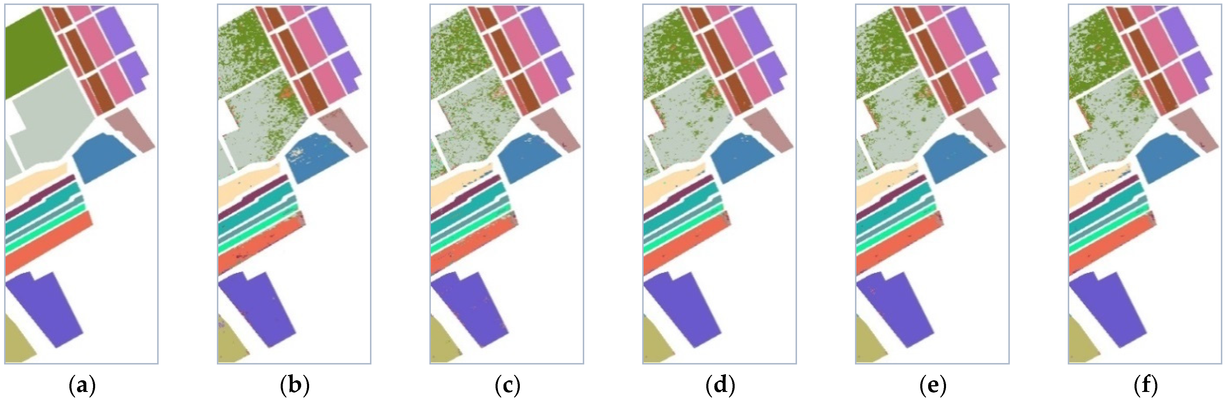
The thematic maps of the Salinas dataset are visually shown in Figure 12b–f. It follows that the proposed DMLOHM algorithm achieved the best classification results for most land cover classes. As for vinyard untrained land cover, most methods inaccurately classified it into grapes untrained land cover while DMLOHM was able to handle this aspect elegantly. The thematic maps of the Pavia University dataset are visually shown in Figure 13b–f. It can be observed that most methods incorrectly classified bare soil into meadow while DMLOHM was found to be a great way to solve this problem. Obviously, by comparing Figure 13e,f, we were able to see that the online hard mining strategy is vital to the DMLOHM method, helping it to achieve a great improvement in results. Simultaneously, the DMLOHM algorithm achieved the best classification results for most land cover classes. Figure 14b–f shows the thematic maps of the HyRANK dataset. We can see that the thematic map of DMLOHM was much closer to the ground truth map. It can effectively distinguish water and coastal water in that the spectral bands of them were found to be similar.
In short, deep metric learning and online hard mining strategy can greatly improve the classification accuracy of the embedded network.
5.4. Time Complexity
The time complexity of DMLOHM was also empirically tested, utilizing 85 training samples per class, which we compared with other approaches. The result in Table 7 shows that DMLOHM consumed a slightly longer period of time than DMLTN because of the extra online hard mining strategy. Although DMLOHM consumed a little more time than DMLTN and CNN, the classification accuracy was significantly improved by 0.14%–4.81%, thus proving that our work is worthy.
6. Discussion
We proposed a deep metric learning-based method aimed at improving dimensionality reduction and limited labeled samples classification accuracy using hyperspectral images in order to achieve good results.
For dimensionality reduction, we utilized a CNN based embedded network to map features into lower-dimensional feature space. However, just using a CNN-based embedded network was not enough. We also utilized an online triplet loss to control the over-fitting or under-overfitting. CNN is originally a good dimensionality reduction tool, and at the same time, we used better sampling strategies to make the network training more targeted, and only used less data to achieve a higher dimensionality reduction effect. The performance of DMLOHM was validated from the aspect of three classification metrics using three datasets The classification accuracy of DMLOHM outperformed other algorithms.
For limited labeled samples classification, both online hard mining strategy and deep metric network played an important part in solving this problem. Deep metric network can effectively make the same class more compact and the heterogeneous more scattered, which made the network better perform classification tasks. Simultaneously, the online hard mining strategy can provide hardest triplets for embedded network to train the whole model. Therefore, the classification accuracy of three datasets showed that our proposed method was better than other algorithms.
Finally, the difference between our proposed method and the others is that other algorithms directly classify hyperspectral data with cross-entropy loss or others, which does not consider the influence of intra-class distance and inter-class distance. Since our algorithm imposes constraints on intra-class distance and inter-class distance, our algorithm improves the classification accuracy obviously.
7. Conclusions
In this paper, we proposed a deep metric learning-based method for hyperspectral classification. Different from the traditional model, we utilized CNN as an embedded network to only extract features. For dimensionality reduction, an embedded CNN network was utilized to map the high-dimensional hyperspectral data to low-dimensional feature space, while online triplet loss was used to constrain the training process of the network, making the model more suitable for hyperspectral data. Online hard mining strategy was utilized to tackle the problem of limited labeled samples classification, which improved the classification accuracy under the condition of limited labeled samples. In future work, we will focus on the classification of spectral features in conjunction with a spatial feature to achieve further superiority in real applications.
Author Contributions
Conceptualization, Y.D. and C.Y.; methodology, Y.D. and C.Y.; writing—original draft preparation, Y.D. and C.Y.; writing—review and editing, Y.D. and Y.Z. All authors have read and agreed to the published version of the manuscript.
Funding
This research was funded by the National Natural Science Foundation of China under Grants 61801444 and 62071438, in part by the State Key Laboratory of Integrated Services Networks (Xidian University) under Grant ISN20-07, and in part by the Hong Kong Scholars Program under Grant XJ2018012.
Institutional Review Board Statement
Not applicable.
Informed Consent Statement
Not applicable.
Data Availability Statement
Data used in this paper can be provided by Cong Yang ([email protected]) upon request.
Acknowledgments
The authors would like to thank the handing editor and all anonymous reviewers for providing insightful and helpful comments.
Conflicts of Interest
The authors declare no conflict of interest.
References
- Scherrer, B.; Sheppard, J.; Jha, P.; Shaw, J.A. Hyperspectral imaging and neural networks to classify herbicide-resistant weeds. J. Appl. Remote Sens. 2019, 13, 044516. [Google Scholar] [CrossRef]
- Tan, K.; Wang, H.; Chen, L.; Du, Q.; Du, P.; Pan, C. Estimation of the spatial distribution of heavy metal in agricultural soils using airborne hyperspectral imaging and random forest. J. Hazard. Mater. 2020, 382, 120987. [Google Scholar] [CrossRef]
- Tuşa, L.; Khodadadzadeh, M.; Contreras, C.; Rafiezadeh Shahi, K.; Fuchs, M.; Gloaguen, R.; Gutzmer, J. Drill-Core Mineral Abundance Estimation Using Hyperspectral and High-Resolution Mineralogical Data. Remote Sens. 2020, 12, 1218. [Google Scholar] [CrossRef] [Green Version]
- Li, X.; Huang, R.; Niu, S.; Cao, Z.; Zhao, L.; Li, J. Local similarity constraint-based sparse algorithm for hyperspectral target detection. J. Appl. Remote. Sens. 2019, 13, 046516. [Google Scholar] [CrossRef]
- Richards, J.A. Clustering and unsupervised classification. In Remote Sensing Digital Image Analysis; Springer: Berlin/Heidelberg, Germany, 2013; pp. 319–341. [Google Scholar]
- Abdi, H.; Williams, L.J. Principal component analysis. Wiley Interdiscip. Rev. Comput. Stat. 2010, 2, 433–459. [Google Scholar] [CrossRef]
- Roweis, S.T.; Saul, L.K. Nonlinear dimensionality reduction by locally linear embedding. Science 2000, 290, 2323–2326. [Google Scholar] [CrossRef] [Green Version]
- Hyvärinen, A.; Oja, E. Independent component analysis: Algorithms and applications. Neural Netw. 2000, 13, 411–430. [Google Scholar] [CrossRef] [Green Version]
- Bennett, K.P.; Demiriz, A. Semi-supervised support vector machines. In Advances in Neural Information Processing Systems; Mitt Press: Cambridge, MA, USA, 1999; pp. 368–374. [Google Scholar]
- Casalino, G.; Gillis, N. Sequential dimensionality reduction for extracting localized features. Pattern Recognit. 2017, 63, 15–29. [Google Scholar] [CrossRef] [Green Version]
- Hinton, G.E.; Salakhutdinov, R.R. Reducing the dimensionality of data with neural networks. Science 2006, 313, 504–507. [Google Scholar] [CrossRef] [Green Version]
- Mika, S.; Ratsch, G.; Weston, J.; Scholkopf, B.; Mullers, K.-R. Fisher discriminant analysis with kernels. In Proceedings of the Neural Networks for Signal Processing IX: Proceedings of the IEEE Signal Processing Society Workshop (Cat. No. 98th8468), Madison, WI, USA, 25–25 August 1999; pp. 41–48. [Google Scholar]
- Baudat, G.; Anouar, F. Generalized Discriminant Analysis Using a Kernel Approach. Neural Comput. 2000, 12, 2385–2404. [Google Scholar] [CrossRef]
- Schölkopf, B.; Smola, A.; Müller, K.-R. Nonlinear Component Analysis as a Kernel Eigenvalue Problem. Neural Comput. 1998, 10, 1299–1319. [Google Scholar] [CrossRef] [Green Version]
- Li, J.; Marpu, P.R.; Plaza, A.; Bioucas-Dias, J.M.; Benediktsson, J.A. Generalized composite kernel framework for hyperspectral image classification. IEEE Transact. Geosci. Remote Sens. 2013, 51, 4816–4829. [Google Scholar] [CrossRef]
- Hughes, G. On the mean accuracy of statistical pattern recognizers. IEEE Trans. Inf. Theory 1968, 14, 55–63. [Google Scholar] [CrossRef] [Green Version]
- Han, J.; Yao, X.; Cheng, G.; Feng, X.; Xu, D. P-CNN: Part-Based Convolutional Neural Networks for Fine-Grained Visual Categorization. IEEE Trans. Pattern Anal. Mach. Intell. 2020, 1. [Google Scholar] [CrossRef]
- Wang, N.; Zha, W.; Li, J.; Gao, X. Back projection: An effective postprocessing method for GAN-based face sketch synthesis. Pattern Recognit. Lett. 2018, 107, 59–65. [Google Scholar] [CrossRef]
- Yuan, X.; Huang, B.; Wang, Y.; Yang, C.; Gui, W. Deep Learning-Based Feature Representation and Its Application for Soft Sensor Modeling With Variable-Wise Weighted SAE. IEEE Trans. Ind. Inform. 2018, 14, 3235–3243. [Google Scholar] [CrossRef]
- Hinton, G.E.; Osindero, S.; Teh, Y.-W. A Fast Learning Algorithm for Deep Belief Nets. Neural Comput. 2006, 18, 1527–1554. [Google Scholar] [CrossRef]
- Mou, L.; Ghamisi, P.; Zhu, X.X. Deep Recurrent Neural Networks for Hyperspectral Image Classification. IEEE Trans. Geosci. Remote Sens. 2017, 55, 3639–3655. [Google Scholar] [CrossRef] [Green Version]
- Hu, W.; Huang, Y.; Wei, L.; Zhang, F.; Li, H.-C. Deep Convolutional Neural Networks for Hyperspectral Image Classification. J. Sens. 2015, 2015, 1–12. [Google Scholar] [CrossRef] [Green Version]
- Makantasis, K.; Karantzalos, K.; Doulamis, A.; Doulamis, N. Deep supervised learning for hyperspectral data classification through convolutional neural networks. In Proceedings of the IEEE International Geoscience and Remote Sensing Symposium (IGARSS), Milan, Italy, 26–31 July 2015; pp. 4959–4962. [Google Scholar]
- Li, Y.; Zhang, H.; Shen, Q. Spectral–Spatial Classification of Hyperspectral Imagery with 3D Convolutional Neural Network. Remote. Sens. 2017, 9, 67. [Google Scholar] [CrossRef] [Green Version]
- Li, W.; Wu, G.; Zhang, F.; Du, Q. Hyperspectral Image Classification Using Deep Pixel-Pair Features. IEEE Trans. Geosci. Remote. Sens. 2016, 55, 844–853. [Google Scholar] [CrossRef]
- Pan, B.; Shi, Z.; Xu, X. MugNet: Deep learning for hyperspectral image classification using limited samples. ISPRS J. Photogramm. Remote. Sens. 2018, 145, 108–119. [Google Scholar] [CrossRef]
- Wu, H.; Prasad, S. Semi-Supervised Deep Learning Using Pseudo Labels for Hyperspectral Image Classification. IEEE Trans. Image Process. 2018, 27, 1259–1270. [Google Scholar] [CrossRef]
- Cheng, G.; Xie, X.; Han, J.; Guo, L.; Xia, G.-S. Remote Sensing Image Scene Classification Meets Deep Learning: Challenges, Methods, Benchmarks, and Opportunities. arXiv 2020, arXiv:2005.01094. Available online: https://0-ieeexplore-ieee-org.brum.beds.ac.uk/document/9127795 (accessed on 30 March 2021). [CrossRef]
- Lu, X.; Sun, H.; Zheng, X. A Feature Aggregation Convolutional Neural Network for Remote Sensing Scene Classification. IEEE Trans. Geosci. Remote. Sens. 2019, 57, 7894–7906. [Google Scholar] [CrossRef]
- Cheng, G.; Yang, C.; Yao, X.; Guo, L.; Han, J. When Deep Learning Meets Metric Learning: Remote Sensing Image Scene Classification via Learning Discriminative CNNs. IEEE Trans. Geosci. Remote. Sens. 2018, 56, 2811–2821. [Google Scholar] [CrossRef]
- Wang, Q.; Wan, J.; Yuan, Y. Locality constraint distance metric learning for traffic congestion detection. Pattern Recognit. 2018, 75, 272–281. [Google Scholar] [CrossRef]
- Weinberger, K.Q.; Saul, L.K. Distance metric learning for large margin nearest neighbor classification. J. Mach. Learn. Res. 2009, 10, 207–244. [Google Scholar]
- Sundermeyer, M.; Schlüter, R.; Ney, H. LSTM neural networks for language modeling. In Proceedings of the Thirteenth Annual Conference of the International Speech Communication Association, Portland, OR, USA, 9–13 September 2012. [Google Scholar]
- Scarselli, F.; Gori, M.; Tsoi, A.C.; Hagenbuchner, M.; Monfardini, G. The Graph Neural Network Model. IEEE Trans. Neural Networks 2009, 20, 61–80. [Google Scholar] [CrossRef] [Green Version]
- Goodfellow, I.; Pouget-Abadie, J.; Mirza, M.; Xu, B.; Warde-Farley, D.; Ozair, S.; Courville, A.; Bengio, Y. Generative adversarial nets. In Advances in Neural Information Processing Systems; Mitt Press: Cambridge, MA, USA, 2014; pp. 2672–2680. [Google Scholar]
- Hoffer, E.; Ailon, N. Deep metric learning using triplet network. In International Workshop on Similarity-Based Pattern Recognition; Springer: Berlin/Heidelberg, Germany, 2015; pp. 84–92. [Google Scholar]
- Hadsell, R.; Chopra, S.; LeCun, Y. Dimensionality reduction by learning an invariant mapping. In Proceedings of the IEEE Computer Society Conference on Computer Vision and Pattern Recognition (CVPR’06), New York, NY, USA, 17–22 June 2006; Volume 2, pp. 1735–1742. [Google Scholar]
- Deng, B.; Jia, S.; Shi, D. Deep Metric Learning-Based Feature Embedding for Hyperspectral Image Classification. IEEE Trans. Geosci. Remote. Sens. 2020, 58, 1422–1435. [Google Scholar] [CrossRef]
- Kaya, M.; Bilge, H. Şakir Deep Metric Learning: A Survey. Symmetry 2019, 11, 1066. [Google Scholar] [CrossRef] [Green Version]
- Bell, S.; Bala, K. Learning visual similarity for product design with convolutional neural networks. ACM Trans. Graph. 2015, 34, 1–10. [Google Scholar] [CrossRef]
- Wang, N.; Gao, X.; Li, J. Random sampling for fast face sketch synthesis. Pattern Recognit. 2018, 76, 215–227. [Google Scholar] [CrossRef] [Green Version]
- Simo-Serra, E.; Trulls, E.; Ferraz, L.; Kokkinos, I.; Fua, P.; Moreno-Noguer, F. Discriminative learning of deep convolutional feature point descriptors. In Proceedings of the IEEE International Conference on Computer Vision, Santiago, Chile, 7–13 December 2015; pp. 118–126. [Google Scholar]
- Schroff, F.; Kalenichenko, D.; Philbin, J. Facenet: A unified embedding for face recognition and clustering. In Proceedings of the IEEE Conference on Computer Vision and Pattern Recognition, Boston, MA, USA, 7–12 June 2015; pp. 815–823. [Google Scholar]
- Manmatha, R.; Wu, C.; Smola, A.J.; Krahenbuhl, P. Sampling Matters in Deep Embedding Learning. In Proceedings of the International Conference on Computer Vision, Venice, Italy, 22–29 October 2017; pp. 2859–2867. [Google Scholar]
- Hermans, A.; Beyer, L.; Leibe, B. In Defense of the Triplet Loss for Person Re-Identification. arXiv 2017, arXiv:abs/1703.07737. Available online: https://arxiv.org/abs/1703.07737 (accessed on 30 March 2021).
- Dong, Y.; Du, B.; Zhang, L.; Zhang, L. Dimensionality reduction and classification of hyperspectral images using ensemble discriminative local metric learning. IEEE Transact. Geosci. Remote Sens. 2017, 55, 2509–2524. [Google Scholar] [CrossRef]
- Li, J.; Huang, X.; Gamba, P.; Bioucas-Dias, J.M.B.; Zhang, L.; Benediktsson, J.A.; Plaza, A. Multiple Feature Learning for Hyperspectral Image Classification. IEEE Trans. Geosci. Remote Sens. 2015, 53, 1592–1606. [Google Scholar] [CrossRef] [Green Version]
- Cao, X.; Ge, Y.; Li, R.; Zhao, J.; Jiao, L. Hyperspectral imagery classification with deep metric learning. Neurocomputing 2019, 356, 217–227. [Google Scholar] [CrossRef]
- Lennon, R. Remote Sensing Digital Image Analysis: An Introduction; Esa/Esrin: Frascati, Italy, 2002. [Google Scholar]
- Dong, Y.; Liang, T.; Zhang, Y.; Du, B. Spectral-Spatial Weighted Kernel Manifold Embedded Distribution Alignment for Remote Sensing Image Classification. IEEE Trans. Cybern. 2020, 1–13. [Google Scholar] [CrossRef]
Figure 1.
Fundamental structure of convolutional neural network (CNN), which consists of a set of layers comprising convolutional layer, pooling layer, and fully connected layer.
Figure 1.
Fundamental structure of convolutional neural network (CNN), which consists of a set of layers comprising convolutional layer, pooling layer, and fully connected layer.

Figure 2.
The flowchart of the proposed method. All hyperspectral pixels with a single shape of are fed into the embedded network separately in order to obtain embedded feature space . From the embedded feature space, the hardest triplets are selected by utilizing a random hardest negative sampling strategy. Finally, all the hardest triplets participate in the calculation of triplet loss in turn and propagate backward to achieve the purpose of obtaining the optimal network parameters.

Figure 3.
Illustration of triplet loss. Anchor, positive sample, and negative sample are projected to the low-dimensional metric space through the model. In each epoch of training, pull the positive sample closer to the anchor while pushing the negative sample far away by triplet loss.
Figure 3.
Illustration of triplet loss. Anchor, positive sample, and negative sample are projected to the low-dimensional metric space through the model. In each epoch of training, pull the positive sample closer to the anchor while pushing the negative sample far away by triplet loss.

Figure 4.
Visualization of Salinas scene. (a) Pseudo-color composite image; (b) ground truth map; (c) land-cover classes.
Figure 4.
Visualization of Salinas scene. (a) Pseudo-color composite image; (b) ground truth map; (c) land-cover classes.

Figure 5.
Visualization of Pavia University dataset. (a) Pseudo-color composite image; (b) ground truth map; (c) land-cover classes.
Figure 5.
Visualization of Pavia University dataset. (a) Pseudo-color composite image; (b) ground truth map; (c) land-cover classes.

Figure 6.
Visualization of Dioni scene. (a) Pseudo-color composite image; (b) ground truth map; (c) land-cover classes.
Figure 6.
Visualization of Dioni scene. (a) Pseudo-color composite image; (b) ground truth map; (c) land-cover classes.

Figure 7.
(a) Classification accuracy of different datasets under different margin values; (b) convergence performances of different training numbers per class in the Pavia University dataset.
Figure 7.
(a) Classification accuracy of different datasets under different margin values; (b) convergence performances of different training numbers per class in the Pavia University dataset.

Figure 8.
Classification accuracy varied as a result of feature dimensions. (a) Salinas dataset; (b) Pavia University dataset; (c) HyRANK dataset.
Figure 8.
Classification accuracy varied as a result of feature dimensions. (a) Salinas dataset; (b) Pavia University dataset; (c) HyRANK dataset.

Figure 9.
The classification performances using different numbers of training samples for the Salinas dataset. (a) overall accuracy (OA); (b) average accuracy (AA); (c) kappa.
Figure 9.
The classification performances using different numbers of training samples for the Salinas dataset. (a) overall accuracy (OA); (b) average accuracy (AA); (c) kappa.

Figure 10.
The classification performances using different numbers of training samples for the Pavia University dataset. (a) OA; (b) AA; (c) kappa.
Figure 10.
The classification performances using different numbers of training samples for the Pavia University dataset. (a) OA; (b) AA; (c) kappa.

Figure 11.
The classification performances using different numbers of training samples for the HyRANK dataset. (a) OA; (b) AA; (c) kappa.
Figure 11.
The classification performances using different numbers of training samples for the HyRANK dataset. (a) OA; (b) AA; (c) kappa.

Figure 12.
Classification results of all the methods for the Salinas dataset. (a) Ground truth map; (b) auto-encoder (AE); (c) recurrent neural network (RNN); (d) CNN; (e) deep metric learning with triplet network (DMLTN); (f) deep metric learning with online hard mining (DMLOHM).
Figure 12.
Classification results of all the methods for the Salinas dataset. (a) Ground truth map; (b) auto-encoder (AE); (c) recurrent neural network (RNN); (d) CNN; (e) deep metric learning with triplet network (DMLTN); (f) deep metric learning with online hard mining (DMLOHM).

Figure 13.
Classification results of all the methods for the Pavia University dataset. (a) Ground truth map; (b) AE; (c) RNN; (d) CNN; (e) DMLTN; (f) DMLOHM.
Figure 13.
Classification results of all the methods for the Pavia University dataset. (a) Ground truth map; (b) AE; (c) RNN; (d) CNN; (e) DMLTN; (f) DMLOHM.

Figure 14.
Classification results of all the methods for the HyRANK dataset. (a) Ground truth map; (b) AE; (c) RNN; (d) CNN; (e) DMLTN; (f) DMLOHM.
Figure 14.
Classification results of all the methods for the HyRANK dataset. (a) Ground truth map; (b) AE; (c) RNN; (d) CNN; (e) DMLTN; (f) DMLOHM.


Table 1.
Land-cover classes and numbers of samples in Salinas dataset.
| Class | Color | Name | Total Number of Samples |
|---|---|---|---|
| C1 | Broccoli green weeds 1 | 2009 | |
| C2 | Broccoli green weeds 2 | 3726 | |
| C3 | Fallow | 1976 | |
| C4 | Fallow rough plow | 1394 | |
| C5 | Fallow smooth | 2678 | |
| C6 | Stubble | 3959 | |
| C7 | Celery | 3579 | |
| C8 | Grapes untrained | 11,271 | |
| C9 | Soil vinyard develop | 6203 | |
| C10 | Corn senesced green weeds | 3278 | |
| C11 | Lettuce romaine 4wk | 1068 | |
| C12 | Lettuce romaine 5wk | 1927 | |
| C13 | Lettuce romaine 6wk | 916 | |
| C14 | Lettuce romaine 7wk | 1070 | |
| C15 | Vinyard untrained | 7268 | |
| C16 | Vinyard vertical trellis | 1807 | |
| Total | 54,129 |
Table 2.
Land-cover classes and numbers of samples in Pavia University dataset.
| Class | Color | Name | Total Number of Samples |
|---|---|---|---|
| C1 | Asphalt | 6631 | |
| C2 | Meadow | 18,649 | |
| C3 | Gravel | 2099 | |
| C4 | Trees | 3064 | |
| C5 | Metal sheets | 1345 | |
| C6 | Bare soil | 5029 | |
| C7 | Bitumen | 1330 | |
| C8 | Bricks | 3682 | |
| C9 | Shadows | 947 | |
| Total | 42,776 |
Table 3.
Land-cover classes and numbers of samples in HyRANK dataset.
| Class | Color | Name | Total Number of Samples |
|---|---|---|---|
| C1 | Dense urban fabric | 1262 | |
| C2 | Mineral extraction sites | 204 | |
| C3 | Non-irrigated arable land | 614 | |
| C4 | Fruit trees | 150 | |
| C5 | Olive groves | 1768 | |
| C6 | Coniferous forest | 361 | |
| C7 | Dense sclerophyllous vegetation | 5035 | |
| C8 | Sparce sclerophyllous vegetation | 6374 | |
| C9 | Sparcely vegetated areas | 1754 | |
| C10 | Rocks and sand | 492 | |
| C11 | Water | 1612 | |
| C12 | Coastal water | 398 | |
| Total | 20,024 |
Table 4.
Classification results for the Salinas dataset with 85 labeled samples per class (about 2.5% of total sample) as the training set (DIM = 128).
Table 4.
Classification results for the Salinas dataset with 85 labeled samples per class (about 2.5% of total sample) as the training set (DIM = 128).
| AE | RNN | CNN | DMLTN | DMLOHM | ||||||
|---|---|---|---|---|---|---|---|---|---|---|
| Class | Mean | Std | Mean | Std | Mean | Std | Mean | Std | Mean | Std |
| C1 | 97.22 | 1.3627 | 98.65 | 1.2857 | 98.65 | 0.6453 | 98.53 | 1.8467 | 99.77 | 0.0483 |
| C2 | 99.34 | 0.9468 | 98.78 | 0.5281 | 99.66 | 0.3874 | 99.07 | 1.1015 | 99.89 | 0.0276 |
| C3 | 95.09 | 2.2834 | 96.93 | 0.9080 | 99.24 | 0.4368 | 99.15 | 0.4288 | 99.92 | 0.1227 |
| C4 | 99.66 | 0.1069 | 99.54 | 0.2178 | 99.71 | 0.0337 | 99.69 | 0.0354 | 99.72 | 0.0538 |
| C5 | 97.67 | 0.7972 | 96.77 | 0.3585 | 98.19 | 0.2418 | 97.13 | 4.2324 | 98.71 | 0.2078 |
| C6 | 99.71 | 0.0832 | 99.58 | 0.3136 | 99.81 | 0.0258 | 99.74 | 0.0493 | 99.79 | 0.0063 |
| C7 | 98.62 | 1.8405 | 99.19 | 0.1535 | 99.48 | 0.0579 | 99.48 | 0.1080 | 99.59 | 0.0658 |
| C8 | 72.35 | 2.3715 | 71.04 | 6.4577 | 80.32 | 2.1563 | 69.80 | 15.0745 | 76.65 | 5.5246 |
| C9 | 98.84 | 0.5185 | 98.80 | 0.3933 | 99.38 | 0.2161 | 99.51 | 0.4952 | 99.89 | 0.0462 |
| C10 | 88.78 | 1.2900 | 86.23 | 1.3433 | 91.33 | 0.5655 | 92.11 | 0.9608 | 96.63 | 0.4062 |
| C11 | 93.61 | 1.4996 | 97.05 | 1.0173 | 97.24 | 0.3975 | 98.34 | 0.7326 | 98.57 | 0.2012 |
| C12 | 98.75 | 1.3655 | 97.34 | 1.5305 | 98.91 | 0.4584 | 99.11 | 0.7789 | 99.90 | 0.0583 |
| C13 | 98.46 | 0.1872 | 98.28 | 0.7329 | 99.23 | 0.2783 | 99.27 | 0.2909 | 99.66 | 0.0759 |
| C14 | 92.86 | 0.9391 | 93.00 | 1.5808 | 97.29 | 0.7526 | 97.52 | 0.5400 | 98.77 | 0.1197 |
| C15 | 63.12 | 3.3930 | 53.36 | 9.3126 | 69.19 | 3.5673 | 74.19 | 16.5001 | 78.20 | 4.5129 |
| C16 | 95.37 | 3.3747 | 96.27 | 1.0644 | 98.43 | 0.1059 | 98.35 | 0.0983 | 98.68 | 0.0705 |
| AA | 93.09 | 0.4580 | 92.54 | 0.3131 | 95.37 | 0.2045 | 95.06 | 0.5061 | 96.52 | 0.0751 |
| OA | 87.27 | 0.0515 | 85.61 | 0.559 | 90.58 | 0.0264 | 89.02 | 1.4321 | 91.63 | 0.0548 |
| Kappa | 0.8582 | 0.0057 | 0.8396 | 0.0061 | 0.8950 | 0.0029 | 0.8779 | 0.0155 | 0.9068 | 0.0059 |
Table 5.
Classification results for the Pavia University dataset with 85 labeled samples per class (about 1.5% of total sample) as the training set (DIM = 128).
Table 5.
Classification results for the Pavia University dataset with 85 labeled samples per class (about 1.5% of total sample) as the training set (DIM = 128).
| AE | RNN | CNN | DMLTN | DMLOHM | ||||||
|---|---|---|---|---|---|---|---|---|---|---|
| Class | Mean | Std | Mean | Std | Mean | Std | Mean | Std | Mean | Std |
| C1 | 67.88 | 3.1520 | 79.21 | 4.0860 | 81.14 | 0.9982 | 81.73 | 3.4160 | 84.15 | 1.4853 |
| C2 | 71.50 | 3.8101 | 76.78 | 3.7735 | 82.94 | 0.9966 | 81.26 | 3.1677 | 86.69 | 1.1915 |
| C3 | 60.87 | 22.9224 | 70.75 | 7.6683 | 78.58 | 6.2574 | 79.49 | 7.7648 | 79.18 | 5.7180 |
| C4 | 91.26 | 2.9592 | 90.90 | 3.2136 | 93.15 | 0.9456 | 94.79 | 1.6010 | 96.63 | 0.3333 |
| C5 | 99.67 | 0.1191 | 99.46 | 0.1206 | 99.88 | 0.0566 | 99.83 | 0.0454 | 99.88 | 0.0566 |
| C6 | 54.00 | 3.8511 | 67.12 | 4.5458 | 76.04 | 1.6330 | 83.66 | 2.9837 | 88.58 | 1.4022 |
| C7 | 90.77 | 1.2038 | 86.57 | 5.4623 | 90.43 | 0.7575 | 91.74 | 2.2630 | 92.87 | 0.9842 |
| C8 | 79.00 | 13.3296 | 81.85 | 3.8278 | 86.08 | 3.3800 | 87.24 | 4.3455 | 86.98 | 6.1821 |
| C9 | 99.99 | 0.0379 | 100.00 | 0.0000 | 99.94 | 0.0632 | 99.98 | 0.0506 | 99.96 | 0.0580 |
| AA | 79.44 | 1.7345 | 83.63 | 1.0873 | 87.58 | 0.3755 | 88.86 | 0.6873 | 90.55 | 0.3262 |
| OA | 72.41 | 0.1329 | 78.61 | 0.1020 | 83.70 | 0.0340 | 84.25 | 1.2638 | 87.73 | 0.5049 |
| Kappa | 0.6459 | 0.0151 | 0.7235 | 0.0114 | 0.7879 | 0.0040 | 0.7967 | 0.0150 | 0.8402 | 0.0062 |
Table 6.
Classification results for the HyRANK dataset with 85 labeled samples per class (about 5.0% of total sample) as the training set (DIM = 128).
Table 6.
Classification results for the HyRANK dataset with 85 labeled samples per class (about 5.0% of total sample) as the training set (DIM = 128).
| AE | RNN | CNN | DMLTN | DMLOHM | ||||||
|---|---|---|---|---|---|---|---|---|---|---|
| Class | Mean | Std | Mean | Std | Mean | Std | Mean | Std | Mean | Std |
| C1 | 61.15 | 6.4555 | 69.48 | 2.0579 | 83.64 | 2.0224 | 80.60 | 2.7210 | 84.15 | 1.6429 |
| C2 | 92.78 | 0.7084 | 93.70 | 1.4948 | 96.56 | 0.6198 | 96.64 | 0.7920 | 97.56 | 0.2656 |
| C3 | 85.99 | 4.3622 | 87.07 | 3.9504 | 93.33 | 0.9224 | 94.08 | 1.2981 | 93.93 | 0.7888 |
| C4 | 97.69 | 2.2052 | 96.92 | 1.9180 | 99.85 | 0.4870 | 100.00 | 0.0000 | 100.00 | 0.0000 |
| C5 | 73.23 | 3.6589 | 72.68 | 4.0310 | 82.90 | 0.8875 | 81.98 | 1.9504 | 84.43 | 0.6411 |
| C6 | 99.35 | 1.1036 | 98.41 | 0.7690 | 100.00 | 0.0000 | 99.93 | 0.1518 | 100.00 | 0.0000 |
| C7 | 89.91 | 0.7151 | 90.31 | 0.9047 | 92.60 | 0.3768 | 91.49 | 0.4103 | 91.22 | 0.3840 |
| C8 | 86.04 | 1.7030 | 84.02 | 1.6785 | 86.47 | 0.8296 | 88.05 | 1.2872 | 86.76 | 0.4438 |
| C9 | 74.09 | 3.8638 | 80.32 | 2.7080 | 90.09 | 0.8269 | 90.20 | 2.6676 | 90.01 | 1.7745 |
| C10 | 94.13 | 2.3209 | 98.60 | 0.7511 | 99.56 | 0.1539 | 99.75 | 0.2310 | 99.68 | 0.2834 |
| C11 | 96.80 | 1.7678 | 98.58 | 1.3699 | 99.91 | 0.1198 | 97.51 | 5.8051 | 99.97 | 0.0827 |
| C12 | 94.15 | 4.1062 | 99.55 | 0.8950 | 98.88 | 0.4588 | 98.91 | 0.8560 | 99.62 | 0.4475 |
| AA | 87.11 | 0.6105 | 89.14 | 0.5744 | 93.65 | 0.1526 | 93.26 | 0.4684 | 93.94 | 0.1763 |
| OA | 84.76 | 0.0624 | 85.56 | 0.0470 | 89.95 | 0.0263 | 89.76 | 0.5770 | 89.89 | 0.2216 |
| Kappa | 0.8091 | 0.0074 | 0.8196 | 0.0057 | 0.8743 | 0.0032 | 0.8718 | 0.0070 | 0.8736 | 0.0027 |
Table 7.
Time consumption (seconds) of different methods.
| Dataset | AE | RNN | CNN | DMLTN | DMLOHM |
|---|---|---|---|---|---|
| Salinas | 251.8425 | 239.5069 | 12.6026 | 19.9895 | 76.5048 |
| Pavia University | 196.8264 | 92.3627 | 7.6125 | 11.8698 | 74.8602 |
| HyRANK | 95.9221 | 90.6688 | 7.2823 | 15.3791 | 74.5944 |
Publisher’s Note: MDPI stays neutral with regard to jurisdictional claims in published maps and institutional affiliations. |
© 2021 by the authors. Licensee MDPI, Basel, Switzerland. This article is an open access article distributed under the terms and conditions of the Creative Commons Attribution (CC BY) license (https://creativecommons.org/licenses/by/4.0/).
Share and Cite
MDPI and ACS Style
Dong, Y.; Yang, C.; Zhang, Y. Deep Metric Learning with Online Hard Mining for Hyperspectral Classification. Remote Sens. 2021, 13, 1368. https://0-doi-org.brum.beds.ac.uk/10.3390/rs13071368
AMA Style
Dong Y, Yang C, Zhang Y. Deep Metric Learning with Online Hard Mining for Hyperspectral Classification. Remote Sensing. 2021; 13(7):1368. https://0-doi-org.brum.beds.ac.uk/10.3390/rs13071368
Chicago/Turabian StyleDong, Yanni, Cong Yang, and Yuxiang Zhang. 2021. "Deep Metric Learning with Online Hard Mining for Hyperspectral Classification" Remote Sensing 13, no. 7: 1368. https://0-doi-org.brum.beds.ac.uk/10.3390/rs13071368
Note that from the first issue of 2016, this journal uses article numbers instead of page numbers. See further details here.