
Quality of Orbit Predictions for Satellites Tracked by SLR Stations


Institute of Geodesy and Geoinformatics, Wrocław University of Environmental and Life Sciences, 50-375 Wrocław, Poland
*
Author to whom correspondence should be addressed.
Remote Sens. 2021, 13(7), 1377; https://0-doi-org.brum.beds.ac.uk/10.3390/rs13071377
Submission received: 24 December 2020
/
Revised: 25 March 2021
/
Accepted: 27 March 2021
/
Published: 3 April 2021
Abstract
:This study aims to evaluate and analyze the orbit predictions of selected satellites: geodetic, Global Navigational Satellite Systems (GNSS), and scientific low-orbiting, which are tracked by laser stations. The possibility of conducting satellite laser ranging (SLR) to artificial satellites depends on the access to high-quality predictions of satellite orbits. The predictions provide information to laser stations where to aim the telescope in search of a satellite to get the returns from the retroreflectors installed onboard. If the orbit predictions are very imprecise, SLR stations must spend more time to correct the telescope pointing, and thus the number of collected observations is small or, in an extreme case, there are none of them at all. Currently, there are about 120 satellites equipped with laser retroreflectors orbiting the Earth. Therefore, the necessity to determine the quality of predictions provided by various analysis centers is important in the context of the increasing number of satellites tracked by SLR stations. We compare the orbit predictions to final GNSS orbits, precise orbits of geodetic satellites based on SLR measurements determined in postprocessing, and kinematic orbits of low-orbiting satellites based on GPS data. We assess the quality degradation of the orbit predictions over time depending on the type of orbit and the satellite being analyzed. We estimate the time of usefulness of prediction files, and indicate those centers which publish most accurate predictions of the satellites’ trajectories. The best-quality predictions for geodetic satellites and Galileo reach the mean error of 0.5–1 m for the whole 5-day prediction file (for all three components), while the worst ones can reach values of up to several thousand meters during the first day of the prediction.
1. Introduction
1.1. SLR
Satellite Laser Ranging (SLR) is an important tool in satellite and space geodesy because it is a technique that can provide independent orbit validation results [1], calibrates the sensors onboard low Earth orbiters, and contributes to generating integrated orbits based on several techniques with a co-location in space [2]. The importance of SLR measurements to assess the quality of the orbits of satellites in low-Earth orbit (LEO), such as Jason-2, Sentinel-3A, CHAMP, GRACE, and Swarm, was discussed by [3]; for the GOCE satellite by [4]; and for the satellites of the Global Navigational Satellite Systems (GNSS) by [5,6,7,8,9].
The International Laser Ranging Service (ILRS, [10]) supports geodetic, remote sensing, navigation, and experimental satellites through performing observations to satellites equipped with retroreflector arrays as well as to reflectors on the Moon. New missions that require SLR tracking can formally submit a request for the ILRS laser ranging tracking support. Thereby, they must meet the guidelines for new missions operated by the ILRS (https://ilrs.gsfc.nasa.gov/missions/mission_support/new_mission_support.html accessed on 30 March 2021). The guidelines also include providing reliable orbit prediction in The Consolidated Prediction Format (CPF/CPF2). The ILRS puts, thus, much emphasis on providing good-quality predictions that are crucial to carrying out measurements by laser stations. However, not all mission operators fulfill the ILRS criteria for high-accuracy orbit predictions, which makes that ILRS station lose time when searching for a satellite with poor-quality predictions.
1.2. Orbit Predictions
To perform laser observations, a laser ranging station must know where a given satellite will be in a given epoch to aim the laser telescope in the right direction while collecting the measurements [11]. If the station hits the satellite, pulses are reflected by the by onboard laser retroreflectors (LRR) and collected by a detector at the ILRS site. Accurate predictions give SLR stations the ability to track, and thus acquire observations. This in turn allows measuring global changes, which are the basic sources of knowledge about the Earth and its dynamics.
A good orbit prediction ensures instant acquisition which means that stations do not lose time in trying to locate the satellite, excellent tracking which means that the telescope is aimed to exactly at the center of the retroreflector, and flat tracks in a narrow range gate which implies no time bias errors in the predicted range [12]. Thanks to good prediction quality, SLR stations can easily track satellites and acquire data with higher yield. Orbit predictions of insufficient quality sometimes prevent SLR observations. An example would be the RadioAstron mission (https://ilrs.gsfc.nasa.gov/missions/satellite_missions/past_missions/radi_support.html accessed on 30 March 2021), for which only three stations were able to conduct laser measurements in the years 2011–2017 the low-quality of orbit predictions. For the LightSail-1 mission (https://ilrs.gsfc.nasa.gov/missions/satellite_missions/past_missions/lita_support.html accessed on 30 March 2021), no measurements could be made until the satellite entered the Earth’s atmosphere. Therefore, the SLR tracking of the LightSail mission failed. In the case of the GOCE mission [4], predictions achieved the precision that allowed for collecting SLR observations, only after optimization of the orbit predictions. For BeiDou satellites of the third generation (-MS1 and -MS2) and geostationary satellites from the second generation, low-quality predictions have been published since the beginning of the tracking campaign, which causes difficulties in performing laser observations (http://sgf.rgo.ac.uk/forumNESC/index.php?PHPSESSID=YUML0TK5KxnRV17XuL1p3rIgi98&topic=43.0&fbclid=IwAR1LoTE_aQGDX9_nlUA-Fj7nLeKklb36WAjAuB1kHPG07WdtSru_xF-1tdU accessed on 30 March 2021).
There are different accuracy requirements for SLR systems. Each of the stations has different equipment, geographic location, or technology employed and operate with a different level of automation. Therefore, it is not possible to provide specific accuracy values that would be appropriate for all SLR stations. The pointing angle error should be lower than half of the transmitted beam divergence at the satellite height to be able to hit the target. The error of the predicted satellite radial component must be smaller than one half of the used range gate width used at the particular SLR station. Therefore, it is impossible to give universal values of orbit error compatible with successful SLR tracking. Some stations can track satellites even when having low-quality orbit predictions. In the case of the GOCE mission, only the Yarragadee station was able to conduct measurements during the last days of the mission due to the low quality of orbit predictions. For the RadioAston mission, only Grasse, Mount Stromlo, and Wettzell managed to track the satellite, whereas only Yarragadee manager to track LightSail-2. None of the SLR stations was able to track LightSail-1 due to the inferior quality of orbit ‘prediction.
Orbit predictions have been published in the (https://ilrs.gsfc.nasa.gov/data_and_products/formats/cpf.html accessed on 30 March 2021) Consolidated Prediction Format (CPF) format since 2008, which is the result of the work of the Prediction Format Study Group, established by the ILRS. This format was intended to provide better quality orbit prediction for artificial satellites, in particular, low-Earth orbiters (LEO). The ILRS collects and publishes data from all prediction providers and for each satellite mission in the public databases (ftp://edc.dgfi.tum.de/pub/slr/cpf_predicts_v2/ accessed on 30 March 2021). Selected ILRS prediction centers are shown in Table 1. CPF files contain the object’s positions and epochs. Furthermore, CPF providers can provide information regarding the accuracy of individual satellite positions in the CPF format. Accuracy of positions is supposed to be determined based on the experience of the prediction providers and is intended to help the station to choose between different providers’ files, as well as to automate the direction detection during the measurement. However, the prediction providers do not supply information about the accuracy of the predicted satellite positions, despite that the CPF format allows for it.
Predicting the satellite orbits is the next step after determining an orbit trajectory using real observations. Having determined orbit parameters, which include Keplerian elements with empirical parameters and taking deterministic perturbations into account, we assume how the satellite positions evolve in later epochs [13]. Therefore, the equation of motion of a satellite must account for the disturbing forces acting on a satellite. These forces may have a gravitational origin, e.g., influence of the gravitational field of the Earth, the Sun or the Moon, Earth’s tides, as well general relativistic effects, and non-gravitational origin, such as atmospheric drag, solar radiation, Earth albedo, thermal forces, antenna thrust. Thus, the equation representing the satellite motion in orbit, including the disturbing forces, can be expressed as [14,15]
where is the acceleration in a geocentric reference frame, is the product of gravitational constant and Earth’s mass, is the position vector of the satellite, is the geocentric range given by , and are the perturbing forces.
The differences between predictions and real satellite trajectories result from inaccuracies in the estimated position and velocity vectors, caused by errors in the orbit determination process (e.g., observation errors, errors in computational procedures), also errors in the numerical integration procedure, mismodeling in the background models, and variabilities of perturbation forces [14]. The influence of the perturbing forces is not constant. It depends primarily on the satellite height above the Earth’s surface. The strongest perturbing force is the atmospheric drag that occurs in the LEO orbit, especially below 800 km. The aerodynamic forces acting on a satellite depend on its geometry, velocity, orientation in relation to the acting force and temperature, and composition and density of the atmosphere, which depend not only on altitude, but also on geographic location, time of year and day, and solar activity or the magnetic field activity. All of these make the correct modeling of the atmospheric drag complicated, which can cause accelerations ranging from to [16].
The predicted satellite positions differ from the actual ones. Consequently, several tools have been developed to deal with this problem. SLR stations use mechanisms to improve the accuracy of prediction. One such method is to search for a target near the prediction position. For this purpose, the stations use algorithms that apply angular search (spiral scan) or search in the “range window”. Stations can also use the time bias offsets to correct for satellite along-track component position because many SLR stations provide real-time time bias offsets. Two services were created publishing the estimated value of the time bias (along-track offsets). The Service Eurostat made it possible to exchange the time bias value in real-time [17,18]. As time-bias values are shown in real-time, the service only works in areas with multiple stations close by such as in Europe. In 2019, the time bias service was created, which collects, calculates, provides, and predicts the time bias data for LEO, geodetic, space debris, and GNSS targets (http://slr.gfz-potsdam.de:5000/tb/v1/ accessed on 30 March 2021). This service enables continuous monitoring of time biases, and hence the quality of satellite orbit predictions. Though, it only provides the along-track offsets, which are the most important from the point of view of SLR stations, and so satellites tracking, while the offsets of the other components are not analyzed [11].
There is a service that provides residuals of the CPF orbit predictions provided by mission operators, which is published by the NERC Space Geodesy Facility (SGF) (http://sgf.rgo.ac.uk/index.html accessed on 30 March 2021). These are comparisons of prediction files coming from two or more prediction centers available. Therefore, it is not possible to determine exactly which file contains data with a higher accuracy. The resulting comparison figures are shown in the Cartesian terrestrial system XYZ, with no transformation to satellite-specific reference frame, so no advanced analyzes can be made on their basis for orbit perturbations.
In order to improve Space Situational Awareness (SSA; an initiative of the European Space Agency (ESA) [19]) it is necessary to track other space targets. Therefore, new methods of accurate target orbits’ prediction are being developed [20,21] aimed at avoiding space hazards, including the collision of satellites with each other or with space debris(http://celestrak.com/events/collision.asp (accessed on 30 March 2021).
1.3. The Goal of the Study
This study analyses the quality of published prediction files dedicated to SLR laser stations for selected satellites in LEO, medium Earth orbit (MEO), and geostationary (GEO) orbits. The research attempts to identify factors affecting the accuracy of orbital predictions to better understand the reasons why observations to some satellites are difficult, with which the ILRS stations are struggling. The obtained results indicate which centers provide more accurate prediction files and what is the degradation of individual components over time. Furthermore, it is a valuable source of information on which of the prediction files need improvement to achieve an accuracy that allows for smooth satellite tracking.
Prediction-related problems formed the basis for conducting research on their assessment. There is little information in existing literature about the accuracy of prediction files, as well as the degradation of prediction quality over time. None of the analyzed files provide any accuracy characteristics regarding generated predictions, meaning that laser station administrators do not know which files to choose for tracking. A random choice of a file containing imprecise data can result in the necessity to conduct manual corrections by the observer. Thus, the analysis described in this article can contribute by saving time on measurements that can be time-consuming or pointless if the predictions used are of poor quality. Such help may prove invaluable in the requirements of the ILRS with a constantly growing list of satellite missions for which SLR measurements are to be conducted.
This article aims at answering the following questions:
- How accurate predictions of satellite orbits are?
- Which prediction providers publish more accurate prediction files?
- What is the degradation of individual orbit components over time for different satellites?
1.4. Structure of the Paper
Section 2 describes the methodology of the analysis. It contains information describing the data used, as well as a description of the data processing scheme. Section 3 discusses the results, which are divided depending on the types of analyzed satellites (geodetic, GNSS, and research LEO). Section 4 provides commentary and summarizes the assessment and analysis of the orbit prediction of selected satellites.
2. Methodology
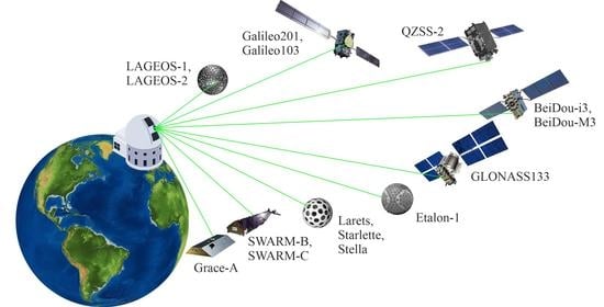
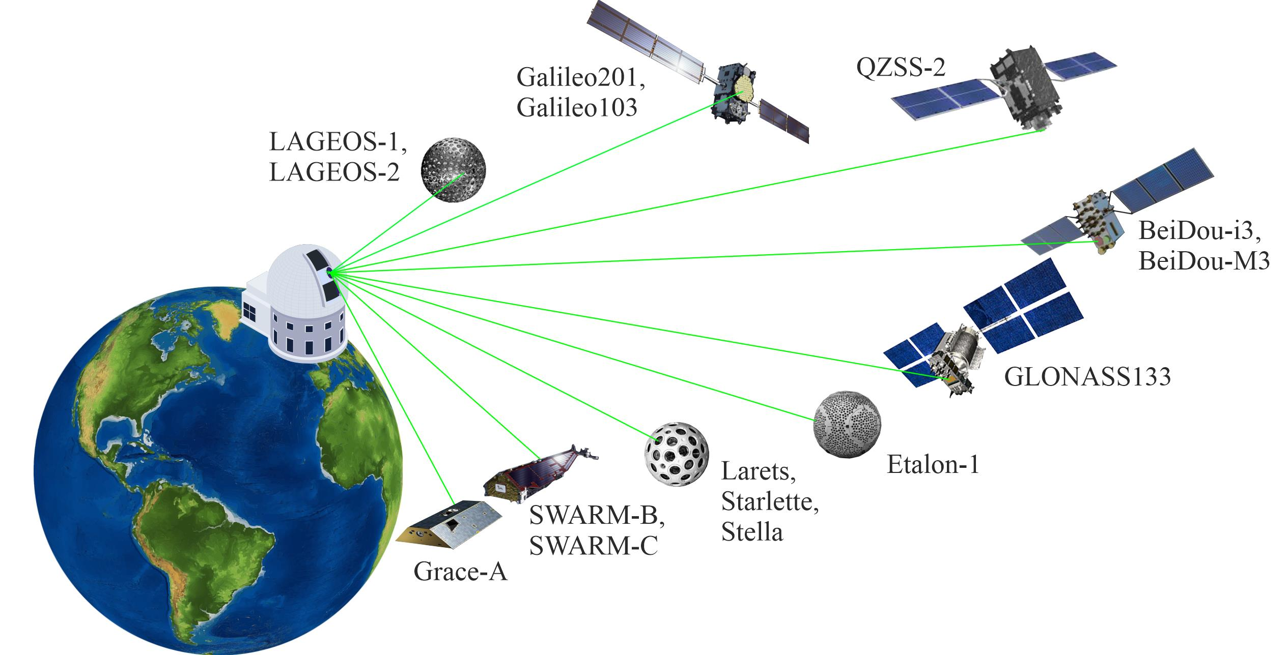
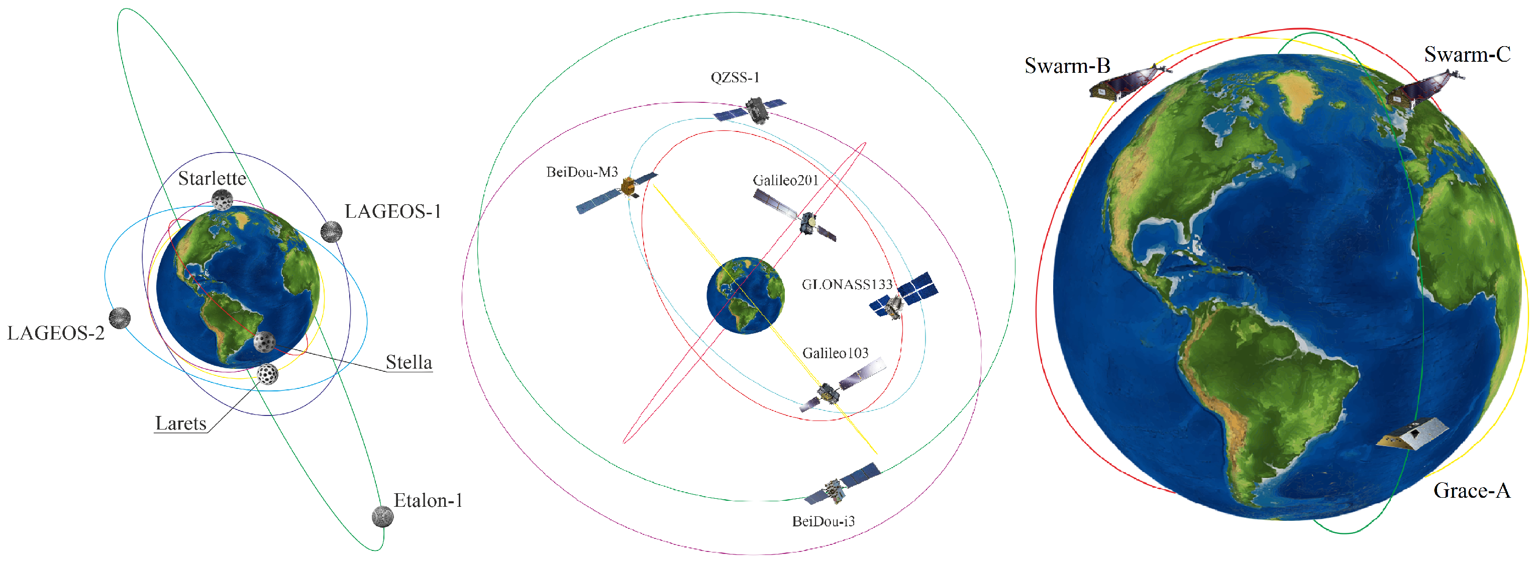
The selection of satellites used in this study was determined by the availability of prediction and precise orbit files. Some precise orbits from various analysis centers were calculated only for a certain period and not on a regular basis. Therefore, the conducted analysis had to refer to this period. Representative time intervals were chosen for the purposes of the analysis so that on this basis it was possible to freely extrapolate the obtained results to other periods. In addition to the availability of predicted and precise orbits, we also considered their construction, orbit characteristics, as well as the influence of the Sun’s height above the orbit plane (the beta angle) and the influence of atmospheric drag (which is correlated with the activity of the Sun). The satellites shown in Figure 1 were selected for analysis. The analyzed “sample” was carefully chosen to represent the whole population as closely as possible. For example, the differences between Glonass 133 and other satellites of this system are negligible because the construction of the satellites is almost the same (e.g., they broadcast signals on three or two frequencies which has a marginal meaning for precise orbit determination). Table 2 (below) shows which satellites of a given system correspond to the satellites selected by us for analysis. On this basis, it is possible to extrapolate the obtained results for a given satellite to a group of satellites.
The choice of analysis periods was closely related to orbit determination errors that change depending on the height of the Sun above the orbit plane (for MEO and GEO), as well as solar activity (LEO). The solar radiation pressure is one of the major perturbing force; therefore, all possible values of the Sun height above the orbital plane were considered. Depending on the inclination, length of a semi-major axis and the eccentricity of the satellite orbits, the draconic period is different (the time interval between two consecutive passes — in the same direction—of the Sun through the orbital plane); therefore, the interval between the analysis periods was selected individually for each satellite. Furthermore, the Sun is at the same height twice during the draconitic period. Analyses were performed for 5 periods lasting 7 days starting from 1 January of a given year. The atmospheric drag values correlate in the thermosphere with the activity of the Sun and the solar cycle causing changes in the upper layers of the atmosphere. These are induced by fluctuations in the level of emitted solar radiation, solar magnetic activity, and streams of charged particles in the form of the so-called solar wind. Changes in the density of the Earth’s thermosphere also indirectly depend on the change in the number and distribution of sunspots. Solar activity is periodic with the primary period of 11 years. Information on space weather is kept up-to-date by the National Oceanic and Atmospheric Administration NOAA (https://www.swpc.noaa.gov/products/solar-cycle-progression accessed on 30 March 2021). Therefore, the analysis for satellites located in LEO orbits has been extended up to two years to include a year with maximum and one with minimum solar activity.
2.1. Predicted Orbits
To improve the accuracy and standardize the prediction format, in June 2006 all analysis centers began to provide satellite orbit prediction files in CPF format, which was the result of 5 years of work by the Prediction Format Study Group, established by the ILRS. The new format replaced the previous one Tuned Inter-Range Vector Range (TIRV). The CPF format was meant to guarantee an improvement in station tracking of more targets both during the day and at night. Moreover, much more sophisticated modeling can be applied by the provider and the prediction quality improved significantly when using CPF [22]. In 2018, the implementation of the updated version started in an ILRS. Currently, the new Consolidated Prediction Format (CPFv2) is in the implementation phase; more information can be found in the EUROLAS data center (https://edc.dgfi.tum.de/en/cpfv2-status/ accessed on 30 March 2021).
The prediction files used in this analysis came from the website of the German Deutsches Geodätisches Forschungs Institut, which is an ILRS data center (ftp://edc.dgfi.tum.de/pub/slr/cpf_predicts/ accessed on 30 March 2021). The files consist of a header, data records, and commentary for a given satellite for a definite time. The header of the file is divided into two parts: the obligatory part (record type H1 and H2), which includes information such as format version, name of the satellite, time to develop the prediction, etc., and the non-required part, in which prediction providers may include an estimate of the expected accuracy (peak-to-peak) at certain points during the day (record type H3). This information is to be provided based on the experience of the prediction provider and is intended to help stations in the context of file selection between individual centers, as well as to automatically set an optimal range gate. Then, there are ephemeris records, where the satellite position vectors are given in meters, and the observation periods in the modified Julian date (MJD) with seconds. For satellites orbiting the Earth, the state vectors are published in the International Terrestrial Reference Frame (e.g., ITRF2014) geocentric frame, based on the best possible force models (gravity field, atmospheric drag, solar radiation pressure, etc.), always referenced to the center of mass of the satellite. The time between satellite positions in the prediction files is constant, typically 1–3 min for LEO orbits and 5–15 min for MEO and GEO orbits. Published files contain several days of data because long predictions help laser stations interpolate over day boundaries, and as a precaution in case of a failure that prevents the center from publishing the file for the next day.
2.2. Precise Orbits
Files containing precise orbits are published in the The Extended Standard Product 3 (SP3) format, which was adopted in 1991 [23], to exchange data regarding satellite orbit and clock information. The SP3 file can carry one of two different sets of satellite orbit parameters; the first, containing orbital ephemeris, or the second, describing the orbit using the Earth’s Cartesian coordinate system. This format consists of a file header containing basic information and subsequent data records. In the header, one can find, among others, information about the file version, type of orbit, time system indicator, number and identifiers of observed satellites, orbit accuracy index, information about the initial and final epoch of observation, as well as about the measuring interval [24]. Files used in this work contained information about the position of the satellite [X Y Z] and, velocity components [Vx Vy Vz] if provided.
2.2.1. Precise Orbits of Geodetic Satellites
The precise orbits for Etalon-1 and LAGEOS-1 and -2 satellites used in this work came from the DGFI website (ftp://edc.dgfi.tum.de/pub/slr/products/orbits/ accessed on 30 March 2021) (the same orbits can be found alternatively on the CDDIS website). Seven-day state vectors of satellites are produced by ILRS Analysis Centers and ILRS Combination Centers as official products since 2016. These orbits are calculated on the basis of data from 7 days of observation and published in the Earth-Centered Earth-Fixed (ECEF) reference system consistent with ITRF2014/SLRF2014 as recommended by the International Earth Rotation and Reference Systems Service (IERS). In the case of Etalon and LAGEOS satellites, the official ILRS-A products were used, which are the combined orbits based on all ILRS Analysis Centers as generated by the ILRS Combination Center hosted by the Italian Space Agency (ASI). The precise orbits for geodetic satellites in low orbits, that is, Larets, Starlette, and Stella, came from research on the contribution of these satellites to the implementation of the international reference system and changes in the Earth’s gravitational field ([25,26]) based on 1-day orbital arcs and generated using models compliant with the IERS 2010 Conventions [27]. Files contain position and velocity vectors in the Earth’s reference system [X Y Z] for a given epoch in UTC with an observation interval of 30 s.
2.2.2. Precise Orbits of Navigation Satellites
GNSS precise orbital products came from the double-difference processing of two-frequency GNSS observations provided by the Center for Orbit Determination in Europe (CODE [28]) as part of the constantly developing Multi-GNSS-Experiment (MGEX [29]). The orbit determination is supported by estimating dedicated solar radiation pressure (SRP) coefficients from the ECOM2 model [30]. The combined solutions are somewhat deficient in developing precise orbit models, in particular for the BeiDou system, in terms on the lack of sufficient knowledge about new systems. Among other things, models of terrestrial radiation pressure (albedo), thermal radiation, or antenna thrust are used only for GPS, GLONASS, and Galileo systems, which may disturb the precision of generated orbits for other systems [31]. Therefore, the same orbit models are employed for the entire GNSS, which is not a fully optimal approach (including using the same orbital arc length for all types of orbits). Precise orbits from CODE are regularly made available with a delay of about two weeks in the SP3 format with an observation interval of 15 min (ftp://ftp.aiub.unibe.ch/CODE_MGEX/CODE/ accessed on 30 March 2021).
2.2.3. Precise Orbits of Research LEO Satellites
The precise orbits of GRACE satellites came from studies on the determination of LEO orbits [32]. The kinematic orbits of GRACE satellites are based on processed GPS observations. Their number allows applying for a geometrical approach in the recovery of satellite positions for the observation epochs using the least-squares method, without using any information about the dynamics of the LEO orbit [33]. In the process of determining the orbit, quick clock corrections [34] and GPS orbits from CODE [35] were used. Precision orbits for Swarm satellites came from the processing of 1.5 years of GPS observations and attitude data for the independent validation of orbits conducted by the Astronomical Institute of the University of Bern in the framework of the ESA’s Swarm Quality Working Group [36]. The final files used in the RL02 (ReLease) analysis contained positions [X Y Z] of satellites with an interval of 3 min in the GPS time system.
2.3. Scheme of Multi-Source Data Processing
For the purpose of this study, in a fully or partially automatic way, we prepared the source code in the Python programming language, which allowed downloading, conversion, coordinate and time system transformation, and finally comparing prediction files with each other or prediction files with files containing precise orbits. After the method is defined, the program (1) compares CPF files between individual centers or (2) compares prediction files with SP3 files. If the user chooses the first method (1), the program will connect to the server with the satellite prediction files and download the proper files. If the user chooses the second method (2), the program will connect to the proper server (depending on the defined satellite) and download the prediction files and file or files with precise orbits, corresponding to the selected period of analysis. The flowchart explaining the stages of the program’s work is shown in Figure 2. In most cases when using SP3 files, the program must download more than one file because they usually contain a one-day orbital arc. In addition to generated charts, the program also calculates statistics for examined files in the form of mean square error and standard deviation, for individual components: radial (R), along-track (S), and cross-track (W), as well as 3D root mean square (RMS) and 3D standard deviation (STD).
Analyses were carried out in the RSW satellite system to verify the accuracy of the tested predictions, in terms of the impact of perturbation forces acting on satellite orbits. Therefore, it was necessary to transform both the prediction files and SP3 files from the terrestrial reference system to the satellite reference system. For this purpose, it was necessary to know the position and velocity in each epoch of observation. Unfortunately, only files with precise orbits of geodetic satellites contained information about the velocity of individual components. For the transformation purposes, the velocities had to be calculated for other types of satellites based on their positions. Assuming a small interval between adjacent epochs, the satellite velocity can be approximated based on the equation
where is velocity vector , r is the position vector , and t is the interval for which the position is recorded. The time system used to define the epochs of observation is nonuniform in all files; therefore, it was necessary to convert the time values to the same system to conduct the comparisons. The time in the prediction files was given as a MJD date with seconds in the coordinated universal time system (UTC), while in SP3 files—the observation periods are described using UTC or the GPS time.
3. Results
3.1. Quality of the Orbit Predictions—Geodetic Satellites
First, we analyzed predictions for geodetic satellites whose orbits are relatively easy to determine becouse of the simple shape, which makes it easy to model the impact of perturbing forces. The spherical structure and the absence of solar panels mean that the perturbation forces acting on the satellite are minimized, and thus the determined orbit predictions do not deteriorate significantly over time. The factor that has a decisive impact on the quality of the geodetic satellites in the LEO region is the number of collected observations, based on which the orbits are determined—in the case of SLR observations they differ depending on the seasons. Due to the adverse atmospheric conditions prevailing in the northern hemisphere in the autumn–winter period, most of the SLR stations cannot observe LEO geodetic satellites, such as Larets, which results in a small number of data. Six geodetic satellites participated in the study: 3 in the MEO orbits and 3 in the LEO orbit (see Figure 1). The choice of these satellites, in addition to the availability of precise orbits, was also dictated by the orbit characteristics, more precisely the satellite height and the inclination angle (Table 3).
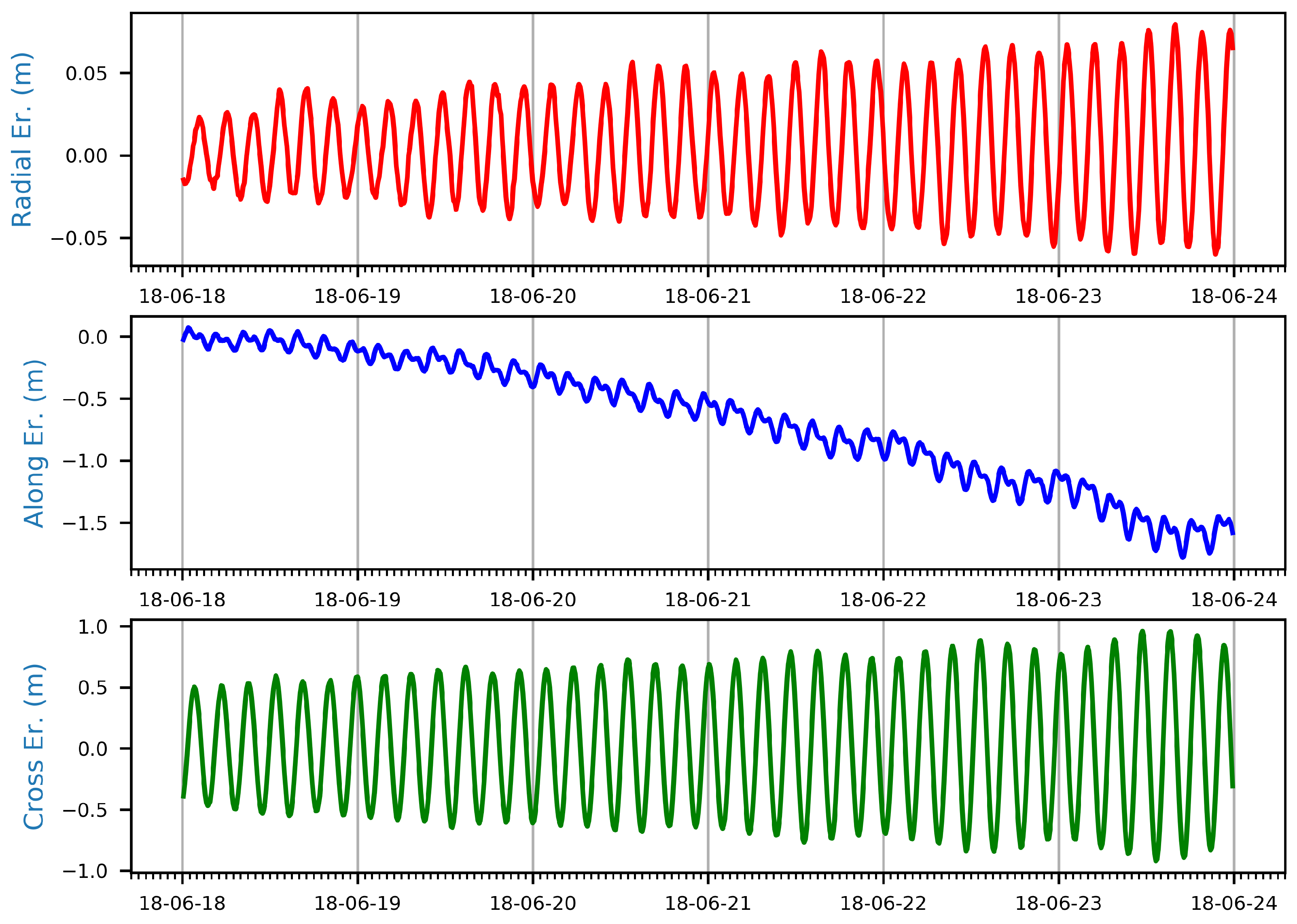
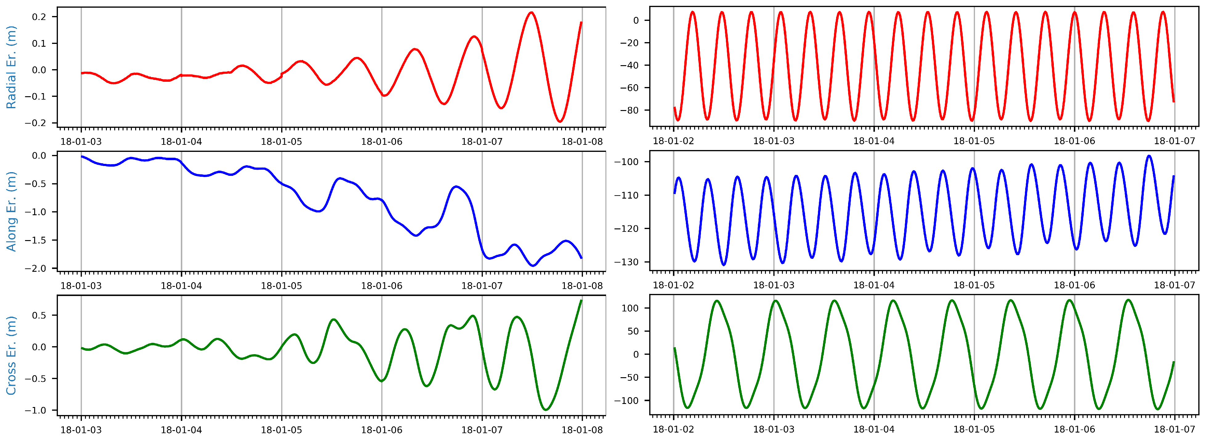
Both the LAGEOS and Etalon satellites are characterized by high-accuracy orbits; therefore, they provide the basis for defining the origin of the terrestrial reference frame. A comparison of CPF and SP3 files shows that the quality of published prediction files for both LAGEOS satellites is similar (see Table 4). In both cases, the provider of the highest accuracy files is the NERC Space Geodesy Facility (SGF). The accuracy of these files is at the level of 0.5 m for the mean square error and standard deviation. The prediction accuracy does not deteriorate significantly over time, as it allows observations for the entire length of the file—5 days. The files provided by the Japan Aerospace Exploration Agency reach a standard deviation and RMS of 1.5 m, and NASA GSFC SLR Mission Contractor files reach the values of several dozen meters (Table 4). Although the LAGEOS satellites have very stable predicted orbits, it can be noticed that the radial and cross-track components for the following days oscillate around zero, while the along-track component additionally fluctuates and drifts away. This is because the along-track is tangent to the velocity vector, and thus it is subject to perturbations related to errors in models describing the Earth’s gravitational field and ocean tides, interaction with the Earth’s magnetic field (induction of eddy currents), thermal effects (e.g., the Yarkovsky effect and the Yarkovsky–Schach effect), or residual atmospheric drag. Additionally, this analysis shows the sinusoidal, typically once-per-revolution nature of the differences between the files containing the predicted and estimated satellite orbits. A number of extreme values in recorded cycles, which can be distinguished for one orbital arc, correspond to the number of satellite revolutions around the Earth. For the LAGEOS satellites, the orbital period is approximately 3 h and 44 min, which translates into almost 6 and a half revolutions in one day, as shown in Figure 3.
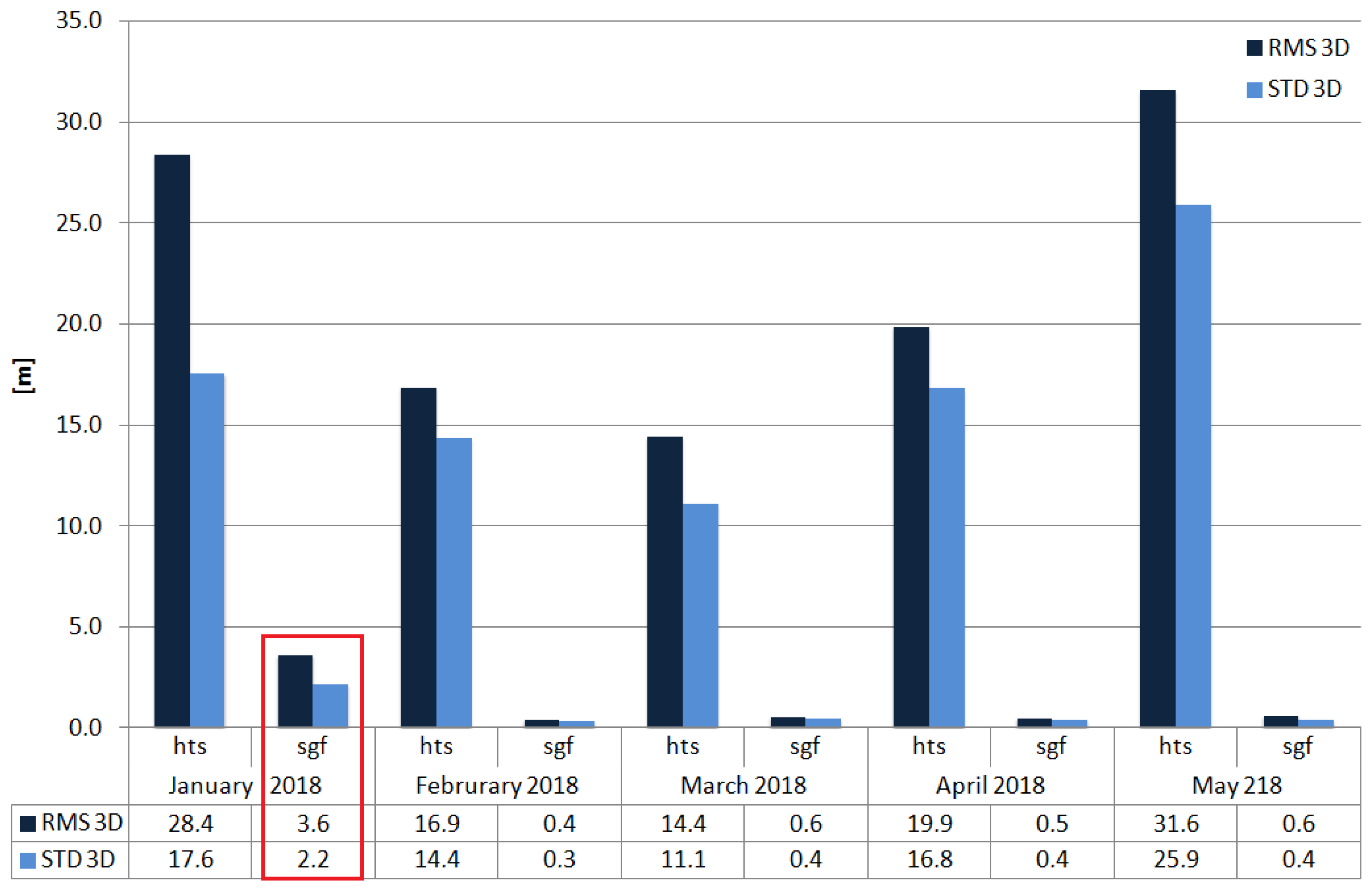
For Etalon satellites, SGF files have the accuracy of 1 m in terms of the mean square error and standard deviation, thus can be recommended as the primary choice of prediction files. Such a difference compared to the LAGEOS satellites is caused by the lower number of Etalon observations in the winter season. As can be seen in Figure 4, the highest values of deviations in relation to SP3 files, for files published by SGF, can be observed in the period of 1–7 January 2018. Apart from the winter period, some laser stations on 1 January do not operate and do not provide any observations. Additionally, for this period there is a large difference between the 3D RMS and STD values, which implies that the mean values of individual components differ significantly from zero. As can be seen in Figure 4, for the remaining analysis periods, the prediction files reach the RMS and STD values analogous to those for the LAGEOS satellites (about 0.5 m).
Subsequent analysis was performed for geodetic satellites in low-Earth orbits: Starlette, Stella, and Larets. In the case of Larets and Stella satellites, the observation geometry is very unfavorable because most SLR stations are located at low or medium latitudes, while the satellites are in sun-synchronous orbits with a high inclination angle, which makes them well observable over the poles and relatively poorly observable over others areas. Therefore, a small number of observations for these satellites is typically recorded: for Stella it is about 30–60% or sometimes even less in relation to the number of measurements for Starlette and about 12% for Larets with the same reference. The results of the comparisons show that the best-predicted orbits are those for the Starlette satellite, published by the NERC Space Geodesy Facility, which does not exceed the value of 15 m (Figure 5). The prediction files published for Stella and Larets satellites show a significant decrease in the quality of the published predictions compared to other geodetic satellites. For both satellites, the worst predicted component is the along-track, indicating that there is a problem with modeling the forces related to atmospheric drag and time-variable gravity field in the LEO orbits. The average values are about 44 m for RMS 3D and almost 30 m for STD 3D for the Stella satellite (files published by the SGF), while for the Larets satellite RMS 3D is 104 m and STD 3D is 67 m based on files published by Mission Control Center, MCC. In the prediction files provided by MCC, the least precise component is the along-track, reaching the mean STD values of 60–80 m, while the radial component oscillates around 1.5–2 m, and the cross-track component is around 5–6 m. Based on the obtained results, it is recommended that only the first day of predicted orbits should be used for geodetic satellites in the LEO orbits.
3.2. Quality of the Orbit Predictions—Navigation Satellites
Quality of the orbit predictions are analyzed for the navigation satellites from four global systems: BeiDou, Galileo, GLONASS, and QZSS (Table 5). Satellites from the GPS system are not included because currently none of the active GPS satellites is equipped with laser retroreflectors. The number of GNSS observations is much higher than the number of SLR observations (the GNSS network consists today of thousands of GNSS reference stations collecting observations from about 40 satellites every second). Moreover, the navigation satellites are in orbits that are not subject to any perturbations caused by the atmospheric drag. Thus, in this case, the main perturbations in satellite orbit determination are direct- and indirect solar-radiation effects, including also albedo and thermal effects. Therefore, eclipsing periods caused by the Earth and the Moon play an important role for the prediction quality. Accurately calculating the shadow coefficient when a satellite enters the umbra or the penumbra area of an occulting body, e.g., the Earth or the Moon, is very important for estimating the satellite acceleration caused by the solar radiation pressure perturbation [37]. The eclipsing periods can be characterized by the value of the angle which represents the angular height of the Sun above the orbital plane.
The prediction providers for Galileo satellites are the European Space Operations Center (ESA) and the Galileo Control Center (GAL). ESA predictions are based on phase GNSS observations collected by a global network of GNSS stations, whereas GAL predictions are based on the satellite telemetry data. The mean RMS and STD values obtained for the differences between CPF and SP3 files vary considerably between the two providers (Figure 6). The prediction files generated by ESA for the Galileo103 satellite reach average RMS and STD 3D values, about 2.0 and 1.5 m, respectively, while for the Galileo201 satellite they are 1.5 and 1.0 m. In addition, the results for the Galileo201 (E18) satellite orbiting in an eccentric orbit are not only highly stable but also better determined than for Galileo103. The high quality of ESA files allows performing observations up to the 5th day in the prediction file, while using files provided by the Galileo Control Center may cause problems in tracking satellites by SLR stations. Predicted satellite positions do not deteriorate in relation to time, but have periodic deviations from the actual satellite position for the entire CPF file. The differences between the prediction files provided by ESA and GAL and the final files are shown in Figure 6. The high stability of the published files in the studied periods implies that the influence of the height of the Sun above the orbital plane does not transfer into the predicted position.
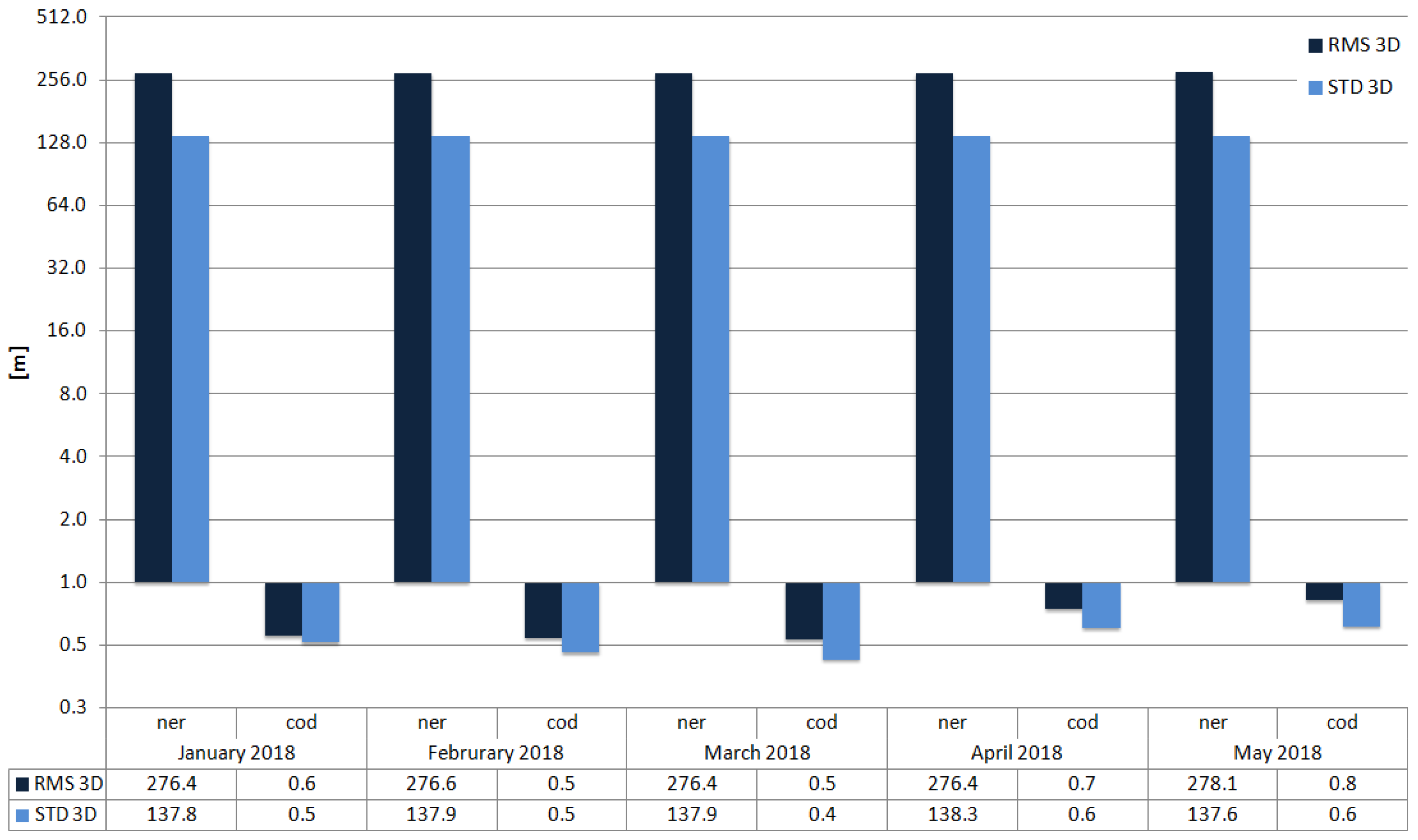
The predictions for the GLONASS133 satellite are published by two centers: the Center for Orbit Determination in Europe (CODE) and the Institute of Space Surveying at the Royal Greenwich Observatory (NERC/NER). The predictions for the GLONASS133 satellite are of high accuracy. The ones provided by CODE achieved RMS and STD values so low, even for 6-day files, that tracking this satellite should not cause any difficulties for stations (Figure 7). Files published by the NER are less accurate and may cause issues for SLR measurements. A significant difference in quality of prediction files, in this case, is most likely caused by modeling used to determinate the orbits. NER uses the same standards for determining the navigation satellites orbit predictions as in the case of geodetic satellites, the so-called cannonball model. This approach is very good for satellites with simple construction (spheres), while for satellites equipped with solar panels, this method seems to be insufficient. The cannonball algorithm does not include the complicated SRP accelerations as the CODE Orbit Empirical Model (ECOM) that is typically employed for GNSS satellites [38,39].
For both BeiDou and QZSS satellites only one center provides prediction files. For BeiDou, it is the center located in the Shanghai Observatory (SHA), and for QZSS it is the Cabinet Office, Government of Japan (QSS). Additionally, files for the BeiDou-M3 and BeiDou-i3 satellites are published every 2–3 days. Orbiting in an inclined geosynchronous orbit, the BeiDou-i3 satellite has more accurate predictions than the BeiDou-M3 satellite in the MEO orbits. For both satellites, no significant changes can be observed when modifying the analysis periods, which means that the orbit predictions are quite robust to the impact of the Sun height above the orbital plane. Both analyzes show that the mean values of RMS and STD are the lowest for the radial component and are about 23 m for the mean square error and 10 m for the standard deviation in the case of the BeiDou-i3 satellite, while for BeiDou-M3 these values are 50 and 7 m, respectively. The cross-track component deviate most from the actual satellite position. Figure 8 shows that difficulties in tracking BeiDou satellites may occur even during the first day of the prediction file. Moreover, the prediction files are not generated every day.
In the case of the QZS-1 satellite predictions, the differences between the predicted and estimated positions reach 50 m for all three components already in the first day of the data file (Figure 8). This can cause difficulties for SLR tracking. The characteristics of the orbits of the QZSS system (inclined eccentric geosynchronous orbit) mean that only five laser stations are capable of performing measurements to these satellites: Tanegashima, Koganei, Yarragadee, Mt. Stromlo, Changchun (https://cddis.nasa.gov/metsovo/docs/PP05B_NAKAMURA_QZSS.pdf accessed on 30 March 2021) (map of SLR stations (https://ilrs.gsfc.nasa.gov/network/stations/index.html accessed on 30 March 2021)). The comparisons show that the predictions for the BeiDou and QZSS satellites are characterized by much lower accuracy than for the Galileo and GLONASS satellites. While predicted orbits of the Galileo or GLONASS satellites achieve the precision of few to dozen meters for the entire file, the ones for BeiDou or QZSS achieve the precision only several dozens to several hundred meters.
3.3. Quality of the Orbit Predictions—Research LEO Satellites
Two of the three Swarm satellites (Bravo and Charlie) and the GRACE-A satellite (Table 6) were also included in this analysis. Such a choice is dictated by the fact that other satellites (Swarm Alpha and GRACE-B) have the same orbits parameters as their twin counterparts. The correctness of the determined orbits for these satellites depends on the quality of atmospheric drag models and space-time variability of the density of the upper layers of the atmosphere or the proper selection of the empirical and stochastic orbit parameters. Therefore, analysis for these satellites was conducted for two time periods in data obtained in two different years, depending on the increased or decreased solar activity.
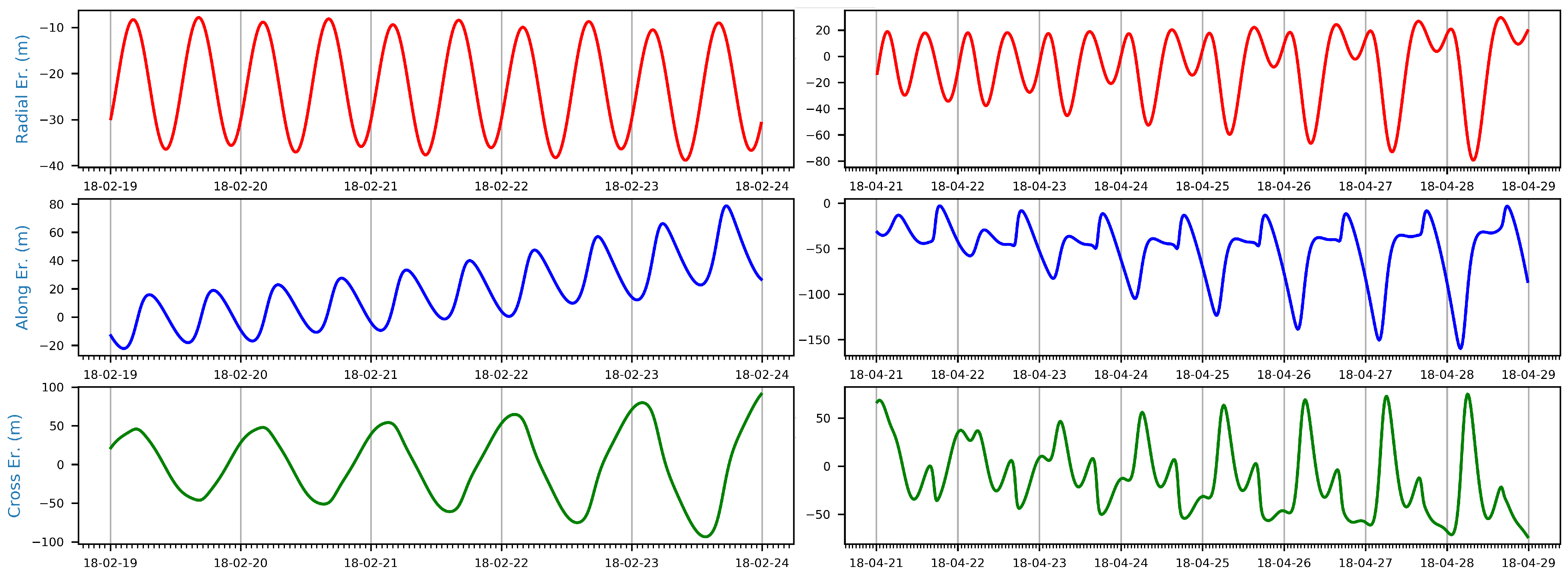
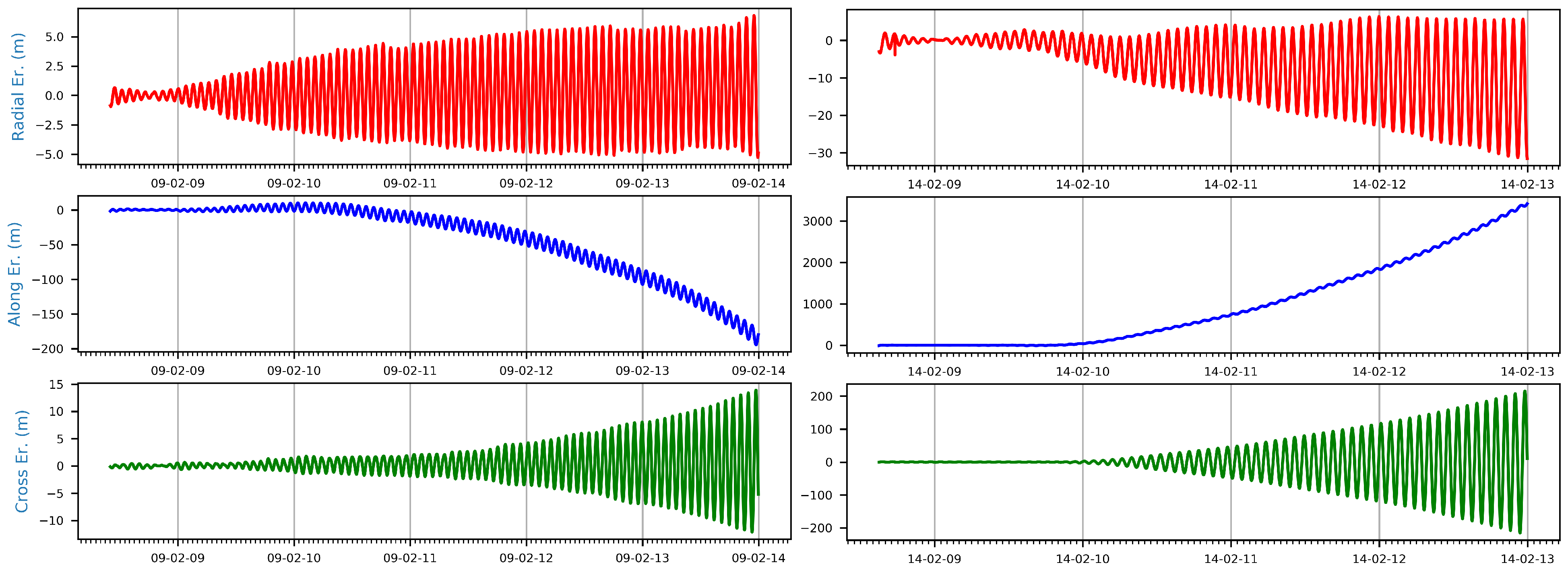
For GRACE satellites, the German Research Centre for Geosciences (GFZ) is the ILRS prediction center, while for Swarm satellites, predictions are provided by ESA. Figure 9 shows comparisons of prediction files with precise GPS-based orbits for the same period in both years with a minimum (2009) and maximum (2014) solar activity. The scales for two figures vary significantly. The along-track component is the worst predicted and reaches the value of 1500 m in 2014 (right) and about 200 m for 2009 (left). For GRACE-A, the accuracy of prediction files depends on the solar activity. In the years when solar activity is low, the first, and partially the second day, allows the SLR stations to track the satellite. While the solar activity is high, practically only the first day of the satellite positions in the prediction file is determined with a sufficient accuracy to enable measurements. For GRACE satellites, there are also some prediction files for which tracking would be impossible without correcting the orbit predictions because the difference between the predicted and the determined position for the along-track component is of the order of several hundred meters even for the first day of the prediction.
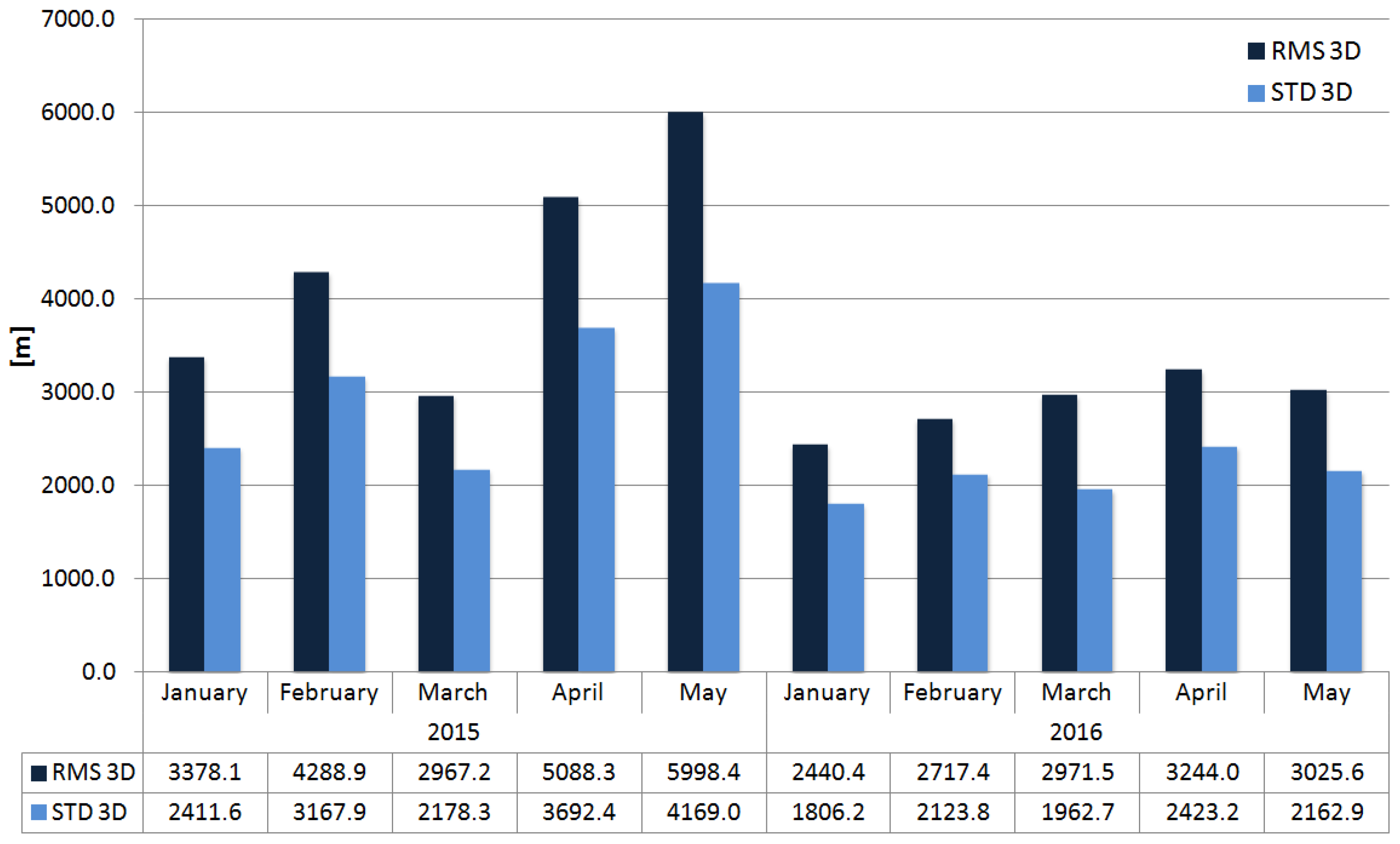
For Swarm satellites in the years with the highest and the lowest solar activity, the analysis of the quality of the predictions is conditioned by the availability of SP3 files, which are provided for 2014–2016. Therefore, analyzes were performed for years 2015 and 2016. For these satellites, there is also a strong relation between the quality of the orbit predictions and the activity of the Sun. The quality of orbit predictions becomes almost twofold lower in 2015 when the activity of the Sun is at its maximum when compared to 2016. In 2016, the solar activity decreased, but did not reach its minimum (see Figure 10). For the early years (2014 and 2015) of the Swarm mission, the orbit solutions were of poor quality. That was caused by ionospheric disturbances affecting the quality of Swarm GPS observations [40,41]. Since 2016, when solar activity decreased and the phase tracking by GPS receivers onboard Swarm satellites has been corrected, the solutions have improved (Figure 10). The usefulness of prediction files ends after about the first prediction day. Using the predicted satellite positions for the second and the consecutive days could turn out to be pointless for SLR stations because of the significant decrease in the precision of the along-track component. The along-track component is characterized by the lowest accuracy, for which RMS reaches values of over 2000 m for the Swarm-B satellite and over 4000 m for the Swarm-C satellite.
4. Discussion and Conclusions
The ability to track satellites by SLR stations depends on the knowledge of the satellite position at the measurement time. The accuracy of satellite orbit predictions directly affects the operation of the ILRS. Due the increasing number of satellite missions with the request for the ILRS support, as well as a small number of SLR observations in the case of some satellites, it was advantageous to assess the quality of orbit prediction provided by various prediction centers. The quality assessment of orbit predictions is also valuable for the purpose of the station operation improvement and data yield.
The analysis of obtained results allows for a selection of prediction centers and prediction files which may be of superior accuracy compared to the others. The list of satellites with prediction providers and mean RMS and STD 3D values is shown in Table 7. The highest values of the RMS and STD were obtained for research LEO satellites ranging from several hundred to several thousand meters after already the first day of the prediction. The best predictions, on the other hand, are for the navigation satellites of the Galileo and GLONASS systems as well as geodetic satellites in medium Earth orbits.
For geodetic satellites in MEO, the accuracy of files varies within 1 m for the RMS and STD and is not significantly deteriorated over time thus, the precision allows observations to be conducted even after 5 days. In the case of satellites in LEO orbits, the quality of predictions is much lower. The prediction accuracy for Starlette and Stella allows performing observations without any correction made by a station observer; the mean STD 3D value is approximately 4 m for Starlette and 18 m for Stella for the entire prediction file. Acquiring observations to the Larets satellite after about 2 days requires corrections. The accuracy of published prediction files primarily depends on the number of SLR observations based on which their orbits are determined. The influence of the external perturbation forces is noticeable only for LEO satellites, for which the precision of the satellite flight trajectory prediction is affected by the atmospheric drag. However, the variation of solar radiation pressure plays a minor role, because the quality of orbit prediction is similar for different heights of the Sun above the orbital planes.
In the case of Galileo and GLONASS satellites, the prediction files’ accuracy is high. The mean standard deviation does not exceed 1 m in files published by ESA and CODE. Prediction files generated for the BeiDou and QZSS satellites are characterized by an inferior accuracy, much exceeding 50 m. The mean root square error for the BeiDou satellites ranges from 60 to 80 m, while for the QZS-1 satellite this value is already about 110 m, so when preparing the data for observation, possible orientation corrections for the laser telescope tracking the satellites should be considered.
The accuracy of orbit predictions of scientific satellites located in a LEO region is the lowest out of all the studied satellites. Perturbation forces have the largest impact on the along-track component, causing its significant degradation, which in extreme cases may reach even several thousand meters. However, the along-track component can be compensated by introducing a time bias. The quality of the prediction is greatly influenced by the atmospheric drag variations which are associated with the solar activity cycle. The variations in the density of the upper atmosphere results in several times greater errors in the determined orbit predictions. For active LEO satellites, it is recommended that the predictions should be constantly monitored and frequently updated even several times a day.
The published satellite orbit prediction files should be unified in terms of the time system used, because in many cases, the time system specified in the CPF file is different from that in which the orbit predictions are given. Now, despite the UTC time system is expected in the files, some predictions are given in the GPS time. A wrongly defined time system makes it much more difficult not only to conduct analyzes, but also causes that laser stations have to control downloaded prediction files before starting observations. Additionally, prediction providers should constantly monitor the maneuvers of satellites in order not to provide predictions for these periods or update predictions just after the maneuver.
Author Contributions
J.N. performed the data analysis and wrote the paper. K.S. edited the manuscript and provided valuable insights. All authors have read and agreed to the published version of the manuscript.
Funding
This work has been supported by the Polish National Science Center (UMO-2019/35/B/ ST10/00515).
Acknowledgments
We acknowledge the ILRS for providing SLR observations, predictionsm and precise LAGEOS/Etalon orbits, as well as AIUB and CODE for providing precise LEO and GNSS orbits.
Conflicts of Interest
The authors declare no conflict of interest.
Abbreviations
The following abbreviations are used in this manuscript:
| GNSS | Global Navigation Satellite System |
| SLR | Satellite Laser Ranging |
| GPS | Global Positioning System |
| LEO | low-Earth orbit |
| ILRS | International Laser Ranging Service |
| LLR | Laser Retroreflector |
| CPF | Consolidated Prediction Format |
| CODE | Center for Orbit Determination in Europe |
| ECOM | empirical CODE orbit model |
| AIUB | Astronomical Institute University of Bern |
| ESOC | European Space Operations Centre |
| GAL | Galileo Control Centre |
| GFZ | German Research Centre for Geosciences |
| HTS | NASA GSFC SLR Mission Contractor, Greenbelt MD, USA |
| JAX | Japan Aerospace Exploration Agency |
| MCC | Mission Control Center, Russia |
| SGF | Space Geodesy Facility |
| QSS | Quazi-Zenith Satellite System Services |
| SSA | Space Situational Awareness |
| ESA | European Space Agency |
| MEO | Medium Earth orbit |
| GEO | Geostationary orbit |
| NOAA | National Oceanic and Atmospheric Administration |
| TIRV | Tuned Inter-Range Vector Range |
| MJD | modified Julian date |
| ITRF | International Terrestrial Reference Frame |
| SP3 | The Extended Standard Product 3 |
| ECEF | Earth-Centered Earth-Fixed |
| IERS | International Earth Rotation and Reference Systems Service |
| ASI | Italian Space Agency |
| UTC | Universal Time Coordinated |
| MGEX | Multi-GNSS-Experiment experiment |
| SRP | Solar radiation pressure |
| SRP Solar radiation pressure R | radial |
| S | along-track |
| W | cross-track |
| RMS | root mean square |
| STD | standard deviation |
| GLONASS | Globalnaja Nawigacionnaja Sputnikovaya Sistema |
| QZSS | Quasi–Zenith Satellite System |
References
- Zajdel, R.; Sośnica, K.; Bury, G. A new online service for the validation of multi-GNSS orbits using SLR. Remote Sens. 2017, 9, 1049. [Google Scholar] [CrossRef] [Green Version]
- Thaller, D.; Dach, R.; Seitz, M.; Beutler, G.; Mareyen, M.; Richter, B. Combination of GNSS and SLR observations using satellite co-locations. J. Geod. 2011, 85, 257–272. [Google Scholar] [CrossRef] [Green Version]
- Arnold, D.; Montenbruck, O.; Hackel, S.; Sośnica, K. Satellite laser ranging to low Earth orbiters: Orbit and network validation. J. Geod. 2018, 1–20. [Google Scholar] [CrossRef] [Green Version]
- Jäggi, A.; Bock, H.; Floberghagen, R. GOCE orbit predictions for SLR tracking. GPS Solut. 2011, 15, 129–137. [Google Scholar] [CrossRef]
- Urschl, C.; Beutler, G.; Gurtner, W.; Hugentobler, U.; Schaer, S. Contribution of SLR tracking data to GNSS orbit determination. Adv. Space Res. 2007, 39, 1515–1523. [Google Scholar] [CrossRef]
- Flohrer, C. Mutual validation of satellite-geodetic techniques and its impact on GNSS orbit modeling. In Geodätisch-Geophysikalische Arbeiten in der Schweiz; Schweizerische Geodätische Kommission: Zurich, Switzerland, 2008; Volume 75, ISBN 978-3-908440-19-2. [Google Scholar]
- Fritsche, M.; Sośnica, K.; Rodríguez-Solano, C.J.; Steigenberger, P.; Wang, K.; Dietrich, R.; Dach, R.; Hugentobler, U.; Rothacher, M. Homogeneous reprocessing of GPS, GLONASS and SLR observations. J. Geod. 2014, 88, 625–642. [Google Scholar] [CrossRef]
- Sośnica, K.; Thaller, D.; Dach, R.; Steigenberger, P.; Beutler, G.; Arnold, D.; Jäggi, A. Satellite laser ranging to GPS and GLONASS. J. Geod. 2015, 89, 725–743. [Google Scholar] [CrossRef] [Green Version]
- Sośnica, K.; Prange, L.; Kaźmierski, K.; Bury, G.; Drożdżewski, M.; Zajdel, R.; Hadaś, T. Validation of Galileo orbits using SLR with a focus on satellites launched into incorrect orbital planes. J. Geod. 2018, 92, 131–148. [Google Scholar] [CrossRef]
- Pearlman, M.R.; Degnan, J.J.; Bosworth, J.M. The international laser ranging service. Adv. Space Res. 2002, 30, 135–143. [Google Scholar] [CrossRef]
- Bauer, S.; Steinborn, J. Time bias service: Analysis and monitoring of satellite orbit prediction quality. J. Geod. 2019, 93, 2367–2377. [Google Scholar] [CrossRef]
- Wood, R. Improving orbit predictions. In Proceedings of the 11th International Laser Ranging Service Workshop, Deggendorf, Germany, 21–25 September 1998; Available online: https://cddis.nasa.gov/lw11/docs/imp_pred.pdf (accessed on 30 March 2021).
- Vetter, J.R. Fifty years of orbit determination. Johns Hopkins Apl Tech. Dig. 2007, 27, 239. [Google Scholar]
- Schutz, B.; Tapley, B.; Born, G.H. Statistical Orbit Determination; Elsevier: Amsterdam, The Netherlands, 2004. [Google Scholar] [CrossRef]
- Combrinck, L. Satellite Laser Ranging. In Sciences of Geodesy-I; Springer: Berlin/Heidelberg, Germany, 2010; pp. 301–338. [Google Scholar] [CrossRef]
- Seeber, G. Satellite Geodesy; (2nd Completely Rev. and Extended ed.); Walter de Gruyter: Berlin, Germany; New York, NY, USA, 2003. [Google Scholar]
- Gurtner, W. Near-real-time status exchange. In Proceedings of the 14th International Laser Ranging Service Workshop, San Fernando, Spain, 7–11 June 2004. [Google Scholar]
- Wood, R.; Gurtner, W. Herstmonceaux/Bern timebias service. In Proceedings of the 13th International Laser Ranging Service Workshop, Washington, DC, USA, 7–11 October 2002. [Google Scholar]
- Bobrinsky, N.; Del Monte, L. The space situational awareness program of the European Space Agency. Cosm. Res. 2010, 48, 392–398. [Google Scholar] [CrossRef]
- Peng, H.; Bai, X. Machine learning approach to improve satellite orbit prediction accuracy using publicly available data. J. Astronaut. Sci. 2020, 67, 762–793. [Google Scholar] [CrossRef]
- Lee, E.; Park, S.Y.; Hwang, H.; Choi, J.; Cho, S.; Jo, J.H. Initial orbit association and long-term orbit prediction for low earth space objects using optical tracking data. Acta Astronaut. 2020, 176, 247–261. [Google Scholar] [CrossRef]
- Ricklefs, R. Consolidated laser ranging prediction format: Field tests. In Proceedings of the 14th International Laser Ranging Service Workshop, San Fernando, Spain, 7–11 June 2004. [Google Scholar]
- Remondi, B.W. NGS Second Generation ASCII and Binary Orbit Formats and Associated Interpolation Studies. In Permanent Satellite Tracking Networks for Geodesy and Geodynamics, Proceedings of the International Association of Geodesy Symposia, Vienna, Austria, 11–24 August 1991; Mader, G.L., Ed.; Springer: Berlin/Heidelberg, Germany, 1993; Volume 109. [Google Scholar] [CrossRef]
- Hilla, S. The Extended Standard Product 3 Orbit Format. 2016. Available online: ftp://igs.org/pub/data/format/sp3d.pdf (accessed on 30 March 2021).
- Sośnica, K.; Jäggi, A.; Thaller, D.; Beutler, G.; Dach, R. Contribution of Starlette, Stella, and AJISAI to the SLR-derived global reference frame. J. Geod. 2014, 88, 789–804. [Google Scholar] [CrossRef] [Green Version]
- Sośnica, K.; Jäggi, A.; Meyer, U.; Thaller, D.; Beutler, G.; Arnold, D.; Dach, R. Time variable Earth’s gravity field from SLR satellites. J. Geod. 2015, 89, 945–960. [Google Scholar] [CrossRef] [Green Version]
- Petit, G.; Luzum, B. IERS Conventions; IERS Technical Note; Verlag des Bundesamts für Kar-tographie und Geodäsie: Frankfurt am Main, Germany, 2010; Volume 58.
- Dach, R.; Schaer, S.; Lutz, S.; Baumann, C.; Bock, H.; Orliac, E.; Prange, L.; Thaller, D.; Mervarta, L.; Jäggi, A.; et al. Center for Orbit Determination in Europe (CODE). In International GNSS Service: Technical Report 2013 (AIUB); Thaller, D., Mervarta, L., Jäggi, A., Eds.; IGS Central Bureau: Pasadena, CA, USA, 2013; pp. 21–34. [Google Scholar]
- Montenbruck, O.; Rizos, C.; Weber, R.; Weber, G.; Neilan, R.; Hugentobler, U. Getting a Grip on Mul-ti-GNSS—The International GNSS Service MGEX Campaign. GPS World 2013, 24, 44–49. [Google Scholar]
- Prange, L.; Orliac, E.; Dach, R.; Arnold, D.; Beutler, G.; Schaer, S.; Jäggi, A. CODE’s five-system orbit and clock solution—The challenges of multi-GNSS data analysis. J. Geod. 2017, 91, 345–360. [Google Scholar] [CrossRef] [Green Version]
- Rodriguez-Solano, C.J.; Hugentobler, U.; Steigenberger, P.; Bloßfeld, M.; Fritsche, M. Reducing the draconitic errors in GNSS geodetic products. J. Geod. 2014, 88, 559–574. [Google Scholar] [CrossRef]
- Jäggi, A.; Hugentobler, U.; Beutler, G. Pseudo-stochastic orbit modeling techniques for low-Earth orbiters. J. Geod. 2006, 80, 47–60. [Google Scholar] [CrossRef] [Green Version]
- Jäggi, A.; Bock, H.; Prange, L.; Meyer, U.; Beutler, G. GPS-only gravity field recovery with GOCE, CHAMP, and GRACE. Adv. Space Res. 2011, 47, 1020–1028. [Google Scholar] [CrossRef]
- Bock, H.; Dach, R.; Jäggi, A.; Beutler, G. High-rate GPS clock corrections from CODE: Support of 1 Hz applications. J. Geod. 2009, 83, 1083. [Google Scholar] [CrossRef] [Green Version]
- Dach, R.; Brockmann, E.; Schaer, S.; Beutler, G.; Meindl, M.; Prange, L.; Bock, H.; Jäggi, A.; Ostini, L. GNSS processing at CODE: Status report. J. Geod. 2009, 83, 353–365. [Google Scholar] [CrossRef] [Green Version]
- Jäggi, A.; Dahle, C.; Arnold, D.; Bock, H.; Meyer, U.; Beutler, G.; van den Jssel, J. Swarm kine-matic orbits and gravity fields from 18 months of GPS data. Adv. Space Res. 2016, 57, 218–233. [Google Scholar] [CrossRef]
- Zhang, R.; Tu, R.; Zhang, P.; Liu, J.; Lu, X. Study of satellite shadow function model considering the overlapping parts of Earth shadow and Moon shadow and its application to GPS satellite orbit determination. Adv. Space Res. 2019, 63, 2912–2929. [Google Scholar] [CrossRef]
- Beutler, G.; Brockmann, E.; Gurtner, W.; Hugentobler, U.; Mervart, L.; Rothacher, M.; Verdun, A. Ex-tended orbit modeling techniques at the CODE processing center of the International GPS Service for geodynamics (IGS): Theory and initial results. Manuscr. Geod. 1995, 19, 367–384. [Google Scholar]
- Arnold, D.; Meindl, M.; Beutler, G.; Dach, R.; Schaer, S.; Lutz, S.; Prange, L.; Sośnica, K.; Mervart, L.; Jäggi, A. CODE’s new solar radiation pressure model for GNSS orbit determination. J. Geod. 2015, 89, 775–791. [Google Scholar] [CrossRef] [Green Version]
- Buchert, S.; Zangerl, F.; Sust, M.; André, M.; Eriksson, A.; Wahlund, J.E.; Opgenoorth, H. SWARM observations of equatorial electron densities and topside GPS track losses. Geophys. Res. Lett. 2015, 42, 2088–2092. [Google Scholar] [CrossRef]
- Sust, M.; Zangerl, F.; Montenbruck, O.; Buchert, S.; Garcia-Rodriguez, A. Spaceborne GNSS-receiving system performance prediction and validation. In Proceedings of the NAVITEC 2014, ESA Workshop on Satellite Navigation Technologies and GNSS Signals and Signal Processing 2014, Noordwijk, The Netherlands, 3 December 2014; pp. 3–5. Available online: http://www.cluster.irfu.se/scb/navitec_2014_sus_et_al_final_for_web.pdf (accessed on 30 March 2021).
Figure 1.
Satellites selected for analysis.

Figure 2.
Scheme of multi-source data processing.

Figure 3.
Comparisons between prediction files from SGF and precise orbits for the period 18–24 June 2018 for the LAGEOS-2 satellite.
Figure 3.
Comparisons between prediction files from SGF and precise orbits for the period 18–24 June 2018 for the LAGEOS-2 satellite.

Figure 4.
RMS and STD values of differences between final and predicted orbits for Etalon-1.

Figure 5.
RMS and STD values of differences between final and predicted orbits for Starlette.

Figure 6.
Comparisons between prediction file and precise orbits for the period 2–7 January 2018 for the Galileo103 satellite for two centers: ESA (left) and GAL (right).
Figure 6.
Comparisons between prediction file and precise orbits for the period 2–7 January 2018 for the Galileo103 satellite for two centers: ESA (left) and GAL (right).

Figure 7.
RMS and STD of differences between final and predicted orbits for GLONASS133. The vertical axis is on a base-2 logarithmic scale.
Figure 7.
RMS and STD of differences between final and predicted orbits for GLONASS133. The vertical axis is on a base-2 logarithmic scale.

Figure 8.
Comparisons between prediction file and precise orbits for the BeiDou-i3 satellite (left) and QZS-1 (right).
Figure 8.
Comparisons between prediction file and precise orbits for the BeiDou-i3 satellite (left) and QZS-1 (right).

Figure 9.
Comparisons between prediction file and precise orbits for two years with the lowest (left) and greatest (right) solar activity for Grace-A.
Figure 9.
Comparisons between prediction file and precise orbits for two years with the lowest (left) and greatest (right) solar activity for Grace-A.

Figure 10.
Comparisons between prediction file and precise orbits for two years with the least (left) and greatest (right) solar activity for Swarm-C.
Figure 10.
Comparisons between prediction file and precise orbits for two years with the least (left) and greatest (right) solar activity for Swarm-C.


Table 1.
List of selected prediction centers providing prediction files for Satellite Laser Ranging (SLR) stations.
Table 1.
List of selected prediction centers providing prediction files for Satellite Laser Ranging (SLR) stations.
| Agency | Abbreviations in CPF Files |
|---|---|
| Center for Orbit Determination in Europe (CODE), Astronomical Institute University of Bern (AIUB) | COD |
| European Space Operations Centre (ESOC) | ESA |
| Galileo Control Centre, DLR, Germany | GAL |
| GFZ German Research Centre for Geosciences | GFZ |
| NASA GSFC SLR Mission Contractor, Greenbelt MD, USA | HTS |
| Japan Aerospace Exploration Agency (JAXA), Japan | JAX |
| Mission Control Center, Russia | MCC |
| NERC Space Geodesy Facility (NSGF), formerly RGO, United Kingdom | NER/SGF |
| Quazi-Zenith Satellite System Services/NEC Corporation | QSS |
| Shanghai, China | SHA |
Table 2.
Satellites selected for analysis and their equivalents.
| Satellites | Total 1 | In Analysis | |||
|---|---|---|---|---|---|
| In Analysis | Equivalent | Analyzed | Equivalent | ||
| Geodesy | Etalon-1 | Etalon-2 | 10 | 6 | 7 |
| LEO | Grace A Swarm C | Grace B Swarm A | 28 | 3 | 5 |
| Navigation | Galileo101 Galileo201 | Galileo102, Galileo103, Galileo104, Galileo203-Galileo222 Galileo202 | 26 | 2 | 26 |
| Glonass133 | All other | 25 | 1 | 25 | |
| BeiDou-i3 BeiDou-M3 | I5, i6b, is1, is2 m1, m2, m9, m10, ms1,ms2 | 14 | 1 1 | 5 7 | |
| QZS1 | QZS2, QZS3, QZS4 | 4 | 1 | 4 | |
| GPS | - | 2 | 0 | 0 | |
| Lunar | - | - | 5 | 0 | - |
| Sum | 120 | 15 | 79 | ||
| Sum of all except the retroreflectors on the Moon and the GPS satellites | 113 | ||||
1 All active satellites which are tracked by the ILRS stations.
Table 3.
Characteristic and periods of analysis of geodetic satellites.
| LAGEOS-1 | LAGEOS-2 | Etalon-1 | Larets | Starlette | Stella | |
|---|---|---|---|---|---|---|
| Type of orbit | MEO | MEO | MEO | LEO | LEO | LEO |
| Inclination [deg] | 109.89 | 52.63 | 64.92 | 97.78 | 49.84 | 98.30 |
| Draconitic year [days] | 561 | 222 | 353.4 | 186.1 | 72.8 | 185.4 |
| Interval [days] | 56 | 22 | 35 | 19 | 7 | 18 |
| Number of years | 1(2018) | 1(2018) | 1(2018) | 1(2015) | 1(2014) | 1(2015) |
Table 4.
Root mean square (RMS) and STD3D values between CPF and SP3 for the LAGEOS-1 satellite.
| LAGEOS-1 | |||||||||||||||
|---|---|---|---|---|---|---|---|---|---|---|---|---|---|---|---|
| 2018 | |||||||||||||||
| January | Februrary–March | April | June | August | |||||||||||
| hts | jax | sgf | hts | jax | sgf | hts | jax | sgf | hts | jax | sgf | hts | jax | sgf | |
| RMS 3D | 17.6 | 1.8 | 0.3 | 10.7 | 1.4 | 0.4 | 88.2 | 1.2 | 0.4 | 24.4 | 0.8 | 0.4 | 20.4 | 2.4 | 0.3 |
| STD 3D | 12.4 | 0.9 | 0.3 | 8.0 | 0.7 | 0.3 | 56.5 | 0.6 | 0.3 | 17.2 | 0.4 | 0.3 | 16.0 | 1.2 | 0.2 |
Table 5.
Characteristic and periods of analysis of Global Navigational Satellite Systems (GNSS) satellites.
Table 5.
Characteristic and periods of analysis of Global Navigational Satellite Systems (GNSS) satellites.
| BeiDou-i3 | BeiDou-M3 | Galileo201 | Galileo101 | GLONASS133 | QZSS-1 | |
|---|---|---|---|---|---|---|
| Type of orbit | IGSO | MEO | MEO | MEO | MEO | GSO 1 |
| Inclination [deg] | 54.42 | 54.83 | 54.94 | 50.16 | 64.92 | 40.83 |
| Draconitic year [days] | 362.3 | 354.6 | 351.6 | 355.6 | 353.4 | 361.4 |
| Interval [days] | 36 | 35 | 36 | 36 | 36 | 36 |
| Number of years | 1(2018) | 1(2018) | 1(2018) | 1(2018) | 1(2018) | 1(2018) |
1 elliptical and inclined geosynchronous orbit.
Table 6.
Characteristic and periods of analysis of scientific satellites.
| GRACE-A | SWARM-B | SWARM-C | |
|---|---|---|---|
| Type of orbit | LEO | LEO | LEO |
| Inclination [deg] | 88.99 | 87.76 | 87.37 |
| Draconitic year [days] | 320.6 | 336 | 336 |
| Interval [days] | 32 | 34(32) | 34(32) |
| Number of years | 2(2009,2014) | 2(2015,2016) | 2(2015,2016) |
Table 7.
List of analyzed satellites and predictions providers that generate files with the most accurate predictions with the mean RMS and STD 3D values based on the entire analysis period.
Table 7.
List of analyzed satellites and predictions providers that generate files with the most accurate predictions with the mean RMS and STD 3D values based on the entire analysis period.
| Satellites | Prediction Centers | RMS 3D [m] | STD 3D [m] |
|---|---|---|---|
| Etalon1 | SGF (or JAX) | 1.1 | 0.8 |
| LAGEOS-1 | 0.4 | 0.3 | |
| LAGEOS-2 | 0.5 | 0.4 | |
| Larets | MCC (or SGF) | 95.3 | 60.4 |
| Starlette | SGF | 6.2 | 4.0 |
| Stella | 25.7 | 17.6 | |
| Galileo103 | ESA/COD | 2.0 | 0.9 |
| Galileo201 | 1.2 | 0.9 | |
| GLONASS133 | COD | 0.6 | 0.5 |
| BeiDou-i3 | SHA 1 | 64.6 | 53.3 |
| BeiDou-M3 | 71.3 | 48.0 | |
| QZS-1 | QSS 1 | 110.0 | 100.1 |
| GRACE-A | GFZ 1 | 832.8 2 | 229.8 2 |
| Swarm-B | ESA 1 | 1109.9 2 | 813.2 2 |
| Swarm-C | 2879.8 2 | 2095.7 2 |
1 For these satellites, the prediction files are published only by one center. 2 For the year with low solar activity.
Publisher’s Note: MDPI stays neutral with regard to jurisdictional claims in published maps and institutional affiliations. |
© 2021 by the authors. Licensee MDPI, Basel, Switzerland. This article is an open access article distributed under the terms and conditions of the Creative Commons Attribution (CC BY) license (https://creativecommons.org/licenses/by/4.0/).
Share and Cite
MDPI and ACS Style
Najder, J.; Sośnica, K. Quality of Orbit Predictions for Satellites Tracked by SLR Stations. Remote Sens. 2021, 13, 1377. https://0-doi-org.brum.beds.ac.uk/10.3390/rs13071377
AMA Style
Najder J, Sośnica K. Quality of Orbit Predictions for Satellites Tracked by SLR Stations. Remote Sensing. 2021; 13(7):1377. https://0-doi-org.brum.beds.ac.uk/10.3390/rs13071377
Chicago/Turabian StyleNajder, Joanna, and Krzysztof Sośnica. 2021. "Quality of Orbit Predictions for Satellites Tracked by SLR Stations" Remote Sensing 13, no. 7: 1377. https://0-doi-org.brum.beds.ac.uk/10.3390/rs13071377
Note that from the first issue of 2016, this journal uses article numbers instead of page numbers. See further details here.