
Registration and Fusion of Close-Range Multimodal Wheat Images in Field Conditions


1
Biosystems Dynamics and Exchanges, TERRA Teaching and Research Center, Gembloux Agro-Bio Tech, University of Liège, 5030 Gembloux, Belgium
2
Plant Sciences, TERRA Teaching and Research Center, Gembloux Agro-Bio Tech, University of Liège, 5030 Gembloux, Belgium
*
Author to whom correspondence should be addressed.
Remote Sens. 2021, 13(7), 1380; https://0-doi-org.brum.beds.ac.uk/10.3390/rs13071380
Submission received: 11 March 2021
/
Revised: 26 March 2021
/
Accepted: 1 April 2021
/
Published: 3 April 2021
(This article belongs to the Special Issue Imaging for Plant Phenotyping)
Abstract
:Multimodal images fusion has the potential to enrich the information gathered by multi-sensor plant phenotyping platforms. Fusion of images from multiple sources is, however, hampered by the technical lock of image registration. The aim of this paper is to provide a solution to the registration and fusion of multimodal wheat images in field conditions and at close range. Eight registration methods were tested on nadir wheat images acquired by a pair of red, green and blue (RGB) cameras, a thermal camera and a multispectral camera array. The most accurate method, relying on a local transformation, aligned the images with an average error of 2 mm but was not reliable for thermal images. More generally, the suggested registration method and the preprocesses necessary before fusion (plant mask erosion, pixel intensity averaging) would depend on the application. As a consequence, the main output of this study was to identify four registration-fusion strategies: (i) the REAL-TIME strategy solely based on the cameras’ positions, (ii) the FAST strategy suitable for all types of images tested, (iii) and (iv) the ACCURATE and HIGHLY ACCURATE strategies handling local distortion but unable to deal with images of very different natures. These suggestions are, however, limited to the methods compared in this study. Further research should investigate how recent cutting-edge registration methods would perform on the specific case of wheat canopy.

1. Introduction
In recent years, close-range multi-sensor platforms and vehicles have been developed for crop phenotyping in natural conditions. The obvious interest of multi-sensor approaches lies in the ability to measure an increased number of pertinent traits. This is especially crucial when studying plant stresses whose symptoms are often complex and not determined by a single physiological or morphological component. For this reason, the philosophy for most modern field phenotyping platforms is to measure both physiological and morphological traits. This requires several types of sensor. On the one hand, spectrometers and 2D imagers provide plant reflectance (visible, near infrared (NIR), thermal IR, etc.) relative to physiological information. On the other hand, 3D cameras and light detection and ranging (LiDAR) devices provide morphological information. Platforms combining such sensors are described in [1,2,3,4,5,6,7]. Each sensor of the platform provides a number of plant traits related to the observed scene. Then, it analyses exploit traits from the different sensors to generate agronomic knowledge. This is what is habitually called “data fusion”. In this generic pipeline, the fusion of information from the different sensors takes place after the extraction of plant traits. However, the complementary nature of the information from the different sensors may also be exploited before that step of traits extraction. This is where the process of images fusion comes into play, as illustrated in Figure 1. Instead of considering separately the images of different cameras (red, green and blue (RGB), monochrome, thermal, depth, …), those images could be fused at the pixel level to enrich the available information [4]. Such a fusion would allow us to segment more finely the images and extract plant traits at a finer spatial scale. Instead of separating only leaves and background, the fusion of data for each pixel may allow us to identify upper leaves, lower leaves, sick tissues, wheat ears, etc. Then, each trait could be computed for those different organs instead of for the whole canopy. This would, for example, solve a well-known issue of close-range thermal imaging: isolating leaves of interest for water status assessment [8]. Image fusion would also allow us to disentangle the effects of leaf morphology and physiology on light reflection. This could be obtained by fusing leaf angles (for example from depth map from stereo camera) and reflectance maps. Such orientation-based reflectance has been suggested to improve thermal imaging by [9]. It is to notice that this paper only envisions the fusion of images, implying that 3D information is provided as a depth map (an image whose pixel values represent distances). The fusion of images and 3D points clouds from LiDAR devices is another hot research topic [10,11,12] but falls outside the scope of this study.
In the context of phenotyping platforms already equipped with different types of camera, multimodal images fusion may be an asset that does not demand supplementary material investment. It offers the possibility to fully benefit from the spatial information brought by imagers, in comparison to non-imaging devices such as thermometers or spectrometers. It also overcomes the disadvantages of mono-sensor multispectral and hyperspectral imagers.
Those mono-sensor spectral devices can be classified into three categories: spatial-scanning, spectral-scanning and filters-matrix snapshot. The spatial-scanning cameras necessitate a relative movement between the scene and the sensor. They are costly [13] and best adapted for indoor applications. Images may be impacted by wind and illumination changes. They have been implemented in the field by, among others, [14,15,16,17]. The spectral-scanning cameras rely on filter wheels [18,19] or tunable filters, i.e., filters whose properties change to allow different spectral bands to pass [20]. Both methods suffer from the same inconvenient as spatial-scanning: the acquisition takes time and is impacted by natural conditions. The filters-matrix snapshot cameras [11] allow simultaneous acquisition of spatial and spectral information, but this comes at the expense of spatial resolution [20]. Unlike these devices, a cameras-array is able to instantly acquire all the spatial and spectral information, that can then be gathered by image fusion.
Despite those many benefits, multimodal image fusion is rarely implemented in close-range systems, due to the difficulty of overlaying the images from the different sensors. This alignment step is called image registration. Considering two images of a same scene acquired by two cameras, the registration consists in geometrically transforming one image (the slave) so that the objects of the scene overlay the same objects in the other image (the master). The registration can be divided into two main steps: the matching between the slave and the master images and the transformation of the slave image. In general, multimodal images registration is a complex problem because the cameras present different spatial positions, different fields of view and different image sizes. Additionally, the multimodal nature of the images implies that they present different intensity patterns, which complicates the matching. In the domain of in-field plant phenotyping, registration is even more challenging due to (i) the nature of the crops (wheat leaves are complex overlapping objects arranged in several floors) and (ii) the natural conditions (sunlight generates shadows and wind induces leaf movement).
Most of the studies that included close-range plants registration concerned thermal and RGB images. It is worth noting that some commercial cameras are able to acquire both RGB and thermal images that are roughly aligned using undocumented registration methods [21]. However, plant researchers relied most of the time on separated cameras and had to deal themselves with the registration step. The most basic approaches were the manual selection of matching points in the slave and master images [8,22] or directly the empirical choice of an unique transformation for all the images [5]. An automatic method was developed by [23] to align thermal and RGB images of side-viewed grapevines. In another study, [9] solved the problem of RGB-thermal registration for maize images. They validated the method using a heated chessboard. The error measured on a simple pattern such as a chessboard may, however, not be representative of the error occurring in a complex crop canopy image. That claim is supported by the fact that the matching is far more complex on plant structures. Even assuming an optimal matching, the different points of view of the cameras may lead to additional errors caused by parallax and visual occlusions. This implies that measuring the registration errors is a difficult task and that the distortion between the images is often complex. None of the plant registration approaches presented above succeeded in taking into account local distortion in the images. Indeed, those approaches relied on global transformations, i.e., functions for which the mapping parameters are the same for the entire image [24]. Nonetheless, the parallax effect alone makes the distortion dependent on the distances of the objects. When acquiring multimodal images from aerial vehicles, this effect is negligible because of the huge distance between the cameras and the scene compared to the displacement of the optical centers and the distance between the objects themselves [25]. At close range, local distortion between the images, and especially parallax effect, may have a significant impact on registration quality. A possible track to solve the issue would be to use a local transformation, i.e., a transformation that is able to locally warp the slave image. The use of such transformations is very scarce in the field of plant sciences but common in other fields such as multimodal medical imaging [26,27]. Local transformations on images of potted-plants were used by [28,29]. To the best knowledge of the authors and at the time of writing, no study has provided a solution for the registration of close-range wheat canopy images. Nevertheless, [30,31] studied wheat images registration under controlled conditions and on isolated potted-plants. They tested three matching methods on side-viewed wheat to align fluorescence and RGB images. The study stuck to a global transformation.
The main objective of this paper is to solve the challenge of automatic registration of close-range multimodal wheat canopy images in field conditions (assuming no targets or markers on the plants). Overcoming this issue is the key to allowing image fusion and open new doors to the processing of multimodal images acquired by modern field phenotyping platforms. In the paper, eight approaches will be studied to relate the slave and master images: one based on a calibration accounting for the cameras system geometry and seven based on the content of the images. Both global and local transformations will be investigated. A rigorous validation of the methods will be performed. Best methods will be highlighted regarding several scenarios and some solutions will be advanced to deal with the remaining alignment errors. The discussion will comment on the performances of matching algorithms and the choice of the transformation model. It will also provide a deeper look at the different natures of distortion between images of a same scene. Finally, it will expand on the challenges of registration quality evaluation.
2. Materials and Methods
2.1. Cameras Set-Up
The multimodal cameras system consisted of a Micro-MCA multispectral cameras array (Tetracam Inc., Gainesville, FL, USA), two GO-5000C-USB RGB cameras (JAI A/S, Copenhagen, Denmark) and a PI640 thermal camera (Optris GmbH, Berlin, Germany). The multispectral array consisted of six monochrome cameras equipped with 1280 × 1024 pixels CMOS sensors. The optical filters were narrow bands centered at 490, 550, 680, 720, 800 and 900 nm. The width of each band-pass filter was 10 nm except for the 900 nm filter that had a width of 20 nm. The lenses had a focal length of 9.6 mm and an aperture of f/3.2. The horizontal field of view (HFOV) was 38.26° and the vertical field of view (VFOV) was 30.97°. The two RGB cameras aimed at forming a stereoscopic camera pair. The baseline (distance between the centers of the two sensors) was 50 mm. Each camera was equipped with a 2560 × 2048 pixels CMOS sensor and a LM16HC objective (Kowa GmbH, Düsseldorf, Germany). Their focal length was 16 mm. The HFOV and VFOV were 44.3° and 33.6°, respectively. The aperture was set to f/4.0. The thermal camera was equipped with a 640 × 480 pixels sensor. It covered a spectral range from 7.5 to 13 μm. The focal length was 18.7 mm. The HFOV and VFOV were 33° and 25°, respectively. The spatial disposition of the cameras is detailed in Figure 2. Their optical axes were theoretically parallel but small deviations were possible due to mechanical imperfections. Each of those vision systems was individually calibrated to remove the geometrical distortions induced by the lenses. The multispectral array was geometrically calibrated using 30 images of a 10 × 7 chessboard (24 mm squares) for each camera. That calibration provided intrinsic camera parameters and coefficients to correct image distortion. The average reprojection error varied between 0.11 and 0.12 pixels depending on the camera. The RGB stereo pair was calibrated using 28 images of the same chessboard. That calibration provided not only intrinsic camera parameters and distortion coefficients but also extrinsic parameters allowing rectification of the images in a context of stereovision. The average error for the camera pair was 0.4 pixels. For the thermal camera, it was not possible to use the chessboard for calibration. A dedicated thermal target was built. That target consisted of a 36 × 28 mm white Forex® plate including 12 removable black-painted disks of 4 cm diameter. The disks were disposed on three rows at regular intervals. The distances between the disks themselves and between the disks and the borders of the plate were 4 cm. Before calibration the plate was stored for 15 min in a freezer at −18 °C and the disks were placed on a radiator. Twenty-three images were acquired during the 10 min after reassembling the target. The algorithm segmented the disks thanks to the temperatures differences. The key points used for calibration (equivalent to the corners of the chessboard in the conventional method) were the centroids of the disk objects. This method was robust to heat diffusion because, regardless of the diameter of the detected hot disks, the centroids were always at the same positions. As for the multispectral cameras array, the calibration provided intrinsic parameters of the camera, including distortion coefficients. The average reprojection error was 0.24 pixels.
Prior to any registration attempt, it was necessary to determine which camera was the master, i.e., the camera providing reference images. The other cameras were considered as slaves. The goal of registration is to find the transformations to apply to slave images so that they are aligned with the master image. The 800 nm camera was chosen as the master. This choice was made because (i) the camera occupied a central position on the sensors pod, (ii) the filter allowed us to segment the images (plant vs. background) and provide plant masks, which are crucial to extract plant traits and (iii) the 800 nm filter clearly highlighted leaves, which could have been important to favor matching. Concerning the two RGB cameras, only one of the two cameras was considered as a slave of the 800 nm master camera: the one that was the closest to it. The images of this RGB camera were cropped to remove the zone not seen by the second RGB camera.
2.2. In-Field Image Acquisition
Images were acquired during the 2020 season in two trial fields located in Lonzée, Belgium (50° 32′ 40′′ N and 4° 44′ 56′′ E). The first trial (trial 1) was planted with winter wheat (Triticum aestivum L. ‘Mentor’) on November 7 2019. The second trial (trial 2) was planted with winter wheat (‘LG Vertikal’) on November 5 2019. Both trials were sowed with a density of 250 grains/m2. The experimental micro-plots measured 1.8 × 6 m2 and the row spacing was 0.15 m. The micro-plots were fertilized three times at BBCH [32] stages 28, 30 and 39 with 27% ammonium nitrate. Trial 1 consisted of eight objects combining contrasted nitrogen inputs. Eight replicates of each object were imaged. Trial 2 consisted of 16 objects combining contrasted nitrogen inputs and fungicide applications (0, 1, 2 or 3 treatments of Adexar® 1.5 l/ha). Four replicates of the objects were imaged. Images of trial 1 were acquired on May 7, May 14, May 20, May 27, June 2, June 11, June 23, July 7 and July 29. Images of trial 2 were acquired on May 12, May 18, June 2, June 9, June 16, June 26, July 13, July 22. At each date and for each camera, four images were taken by micro-plot except for half of the trial 1 replicates (dedicated to punctual destructive measurements) for which only two images were taken. The phenotyping-platform was designed to capture nadir frames of wheat micro-plots. The sensors pod was installed on a cantilever beam to avoid shadows from the rest of the platform in the images. The height of that pod was adjusted at each acquisition date to keep a distance around 1.6 m between the cameras and the top of the canopy. The choice of this distance was a trade-off. On the one hand, the height of the cameras had to be limited so that it was suitable for a proxy-sensing platform and yielded images with a high spatial resolution. On the other hand, the height had to be sufficient to diminish the impact of the difference of point of view on images registration and to screen wide areas that account for plot heterogeneities. At 1.6 m, the footprint of the frames was 0.98 m2 for the cameras of the multispectral array, 1.26 m2 for the RGB cameras and 0.67 m2 for the thermal camera. Images were recorded using a color depth of 10 or 12 bits per pixel but reduced to 8 bits per pixel for this study (because many stereovision and registration open-source libraries need 8-bit inputs). The auto-exposure algorithms of RGB and multispectral devices were adapted to prevent image saturation. The cameras were asked to capture images at the same time but only the two RGB cameras were triggered perfectly together thanks to an external trigger from an Arduino Uno micro-controller. Considering all the cameras, the absence of common external trigger and the different needs in terms of integration time resulted in images acquired with a slight temporal shift. The maximum shift was less than a second.
2.3. Calibration-Based Registration Method
That first image registration method is based on the hypothesis that, for a given configuration of cameras, the best global transformation to register images only depends on the distance between the objects of interest in the scene and the cameras. It relies on a calibration step to establish the distance dependent transformation matrix (DDTM) between the images. This DDTM allows us to express the coefficients of a global transformation as distance-dependent functions [33]. To be as general as possible, the considered approach was the global transformation with the most degrees of freedom, i.e., a homography. This transformation takes into account rotation, translation, shear and scale. Moreover, the scale factors depend on the pixel position in the image which allows us to deal with perspective differences [25]. It gives:
where and are the registered coordinates of a pixel of coordinates x and y in a slave image, d is the distance of the object of interest and hij are the eight independent coefficients of the transformation matrix.
The calibration step was performed in laboratory by capturing the thermal calibration target (described in Section 2.1) at distances ranging from 1 m to 2.2 m by steps of 0.05 m. As the removable disks were of different temperature and of different color that the main body of the target, it was possible to detect the centroids of the disks in images from all the cameras. Those centroids served as key points to determine the best transformation at each distance (Figure 3).
For each camera, the values of the eight coefficients providing the best transformations were related to the distance of the target using linear regressions. An example of such relation is given in Figure 4 for the DDTM that linked the thermal images to the master images. The same trend was observed for all the cameras. Only and significantly varied with distance. For the regressions corresponding to the 490, 550, 680, 720, 900, RGB and thermal cameras, the determination coefficients (R2) were respectively 0.00 (no change with distance), 0.85, 0.65, 0.86, 0.79, 0.01 and. 0.94. The root mean squared errors (RMSE) were, respectively, 5.2, 8.4, 7.1, 7.7, 4.8, 8.6 and 4.2 pixels. For the regressions, R2 were respectively 0.75, 0.03, 0.0, 0.84, 0.86, 0.81 and 0.90. The RMSE were respectively 5.9, 8.0, 8.1, 5.1, 4.5, 7.4 and 2.7 pixels. The other coefficients were approximated to constants by considering the median of the measured values. and of all the matrices were close to 0, which is the case in an affine transformation matrix. This implies that the affine transformation model could have been used.
Applying the DDTM method to field images required measurements of median distances of wheat elements. For the images acquired before heading stage (BBCH50), that distance was measured by stereovision. For the images acquired after heading stage, that distance was approximated based on manual measurements using a stick meter. In that scenario, instead of computing the median distance of wheat for each micro-plot, the approximation was used for all the plots. This choice was made because of the uncertainty on stereovision performances on the various images containing ears (green ears, yellow ears, tilted ears, …). Concerning stereovision applied to wheat canopy, detailed explanations can be found in [34]. For this study, rectification of left and right images was performed by Bouguet’s algorithm thanks to the calibration values extracted using the chessboard [35]. Rectified images were converted to grayscale and reduced to 1280 × 1024 pixels by averaging the pixel intensities on 2 × 2 squares. Matching was performed using the semi-global block matching algorithm [36]. For this algorithm, matching window size was 5 and uniqueness ratio was 10. The median height was computed on segmented plant objects. Segmentation of wheat and background was performed by a threshold of 0.05 on the Excess Red index (ExR). The index was built as follows:
where R, G and B are the intensity values of red, green and blue channels for each pixel.
2.4. Image-Based Registration Methods
Instead of deducing the transformation from the relative positions of the cameras, those methods exploit similarities between the contents of the slaves and the master images to find the best transformation. They do not need a calibration although some of them need prior information on the transformation or initial alignment. They allow us to take into account the nature of the scene. The diversity of images-based registration methods are described in existing reviews [24,37]. An overview of the registration pipeline and of the different methods is presented in Figure 5. The first step of registration is called the matching (Figure 5. Step I). The aim is to detect corresponding zones in the master and the slave images. That correspondence may be feature-based or area-based. In feature-based methods, the goal is to identify a set of features (points, lines or patterns). The sets of features of the slave and the master images are compared to find matches. Popular methods exploit point features that are robust to scale and rotation changes. In the area-based methods, no features are detected. The matching between the images (or two windows from those images) is performed through the maximization of a similarity metric such as cross-correlation coefficient or mutual information. After establishing a correspondence, the second step of registration is to determine the geometric transformation to apply to the slave image (Figure 5. Step II). Transformations are divided into global and local methods. Global methods use the same mapping parameters for the entire image while the local methods are various techniques designed to locally warp the image. If there is no distortion between the images, rotation and translation are sufficient to align them. Otherwise, hypotheses on the distortion should be established to select either another global transformation (similarity, affine, homography) or a local transformation. For complex distortion, a possible approach is to begin with a global transformation and then to refine the registration using one or several local methods. Once coordinates in the slave image have been remapped, the last step consists in resampling the image to compute the new intensities (Figure 5. Step III). It involves convolutional interpolation algorithms such as nearest neighbors, bilinear (based on four neighbors) or cubic (based on 16 neighbors) [37]. Despite the development of more complex resampling approaches slightly outperforming the traditional ones, it is often sufficient to stick to the simple bilinear or cubic algorithm [24]. Registration approaches are mainly differentiated by the choice of the matching method and of the transformation model.
The registration methods tested in the frame of this study are summarized in Table 1 (also including the DDTM calibration-based method). The idea was to test methods that rely on open-source algorithms and libraries so that they can be easily implemented by all plant sciences stakeholders. The programming language was Python 3.7. Four popular methods relying on features-based matching and global transformations were tested from the famous OpenCV library [35] (version 4.1.0.25). Those methods were SIFT [38], SURF [39], ORB [40] and A-KAZE [41]. Default parameters were used for features detection. Then, the matches were sorted by score and only the best matches were kept to compute the transformation. That proportion of valid matches was considered as a sensitive parameter and a sensitivity study was led to identify the best value for each method and each camera. In addition of those features-based methods, three area-based methods were also tested. The first method, referred to as DFT, exploited a discrete Fourier transform to compute a correlation metric in the frequency domain [42]. It was implemented using the imreg_dft Python library (version 2.0.0). The second method, named ECC, relied on a similarity metric built using an enhanced correlation coefficient [43]. It was implemented using Python OpenCV library (version 4.1.0.25). The third area-based method, called B-SPLINE, used a normalized mutual information (NMI) metric and differentiated itself from all the others by performing a local transformation of the slave image. That method was implemented using the Elastix library, initially developed for medical applications [26]. For Python, the library wrapper was pyelastix (version 1.2). This allowed a local transformation based on a 3rd-order (cubic) B-SPLINE model [44]. In addition, the NMI metric is recognized to be particularly suitable for multimodal images registration [24,26,27,45,46]. However, the main drawback of area-based methods is that they may necessitate an initial alignment if the slave images underwent transformations such as huge rotation or scaling. For this reason, the calibration-based DDTM method was exploited to provide roughly registered images before applying the DFT, ECC and B-SPLINE methods. In the end, aligned slave images were cropped to save 855 × 594 pixels images that were limited to the commonly aligned zone. Considering the cameras at 1.6 m height, that zone represented an area of 0.38 m2.
2.5. Validation of the Registration Methods
The evaluation of registration performances is a difficult task and each method has its drawbacks. For this reason, three different indicators were employed:
- The percentage of plausible alignments. This indicator assessed the number of images that seemed visually aligned. It was computed by a human operator examining the registered images in a viewer, beside their master image, one by one. Bad automatic registrations were characterized by aberrant global transformations that were easy to identify (Figure 6). For the local transformation, alignments were considered aberrant in case of the apparition of deformed black borders in the frame or illogical warping of objects such as leaves curving in complete spirals. That indicator was computed for all the acquired images, i.e., a total of 3968 images for each camera.
- The average distance between control points in aligned slave and master images (control points error) [23]. The control points were visually selected on the leaves and ears by a human operator. The points had to be selected on recognizable pixels. Attention was paid to select them in all images regions, at all canopy floors and at different positions on the leaves (edges, center, tip, etc.). It was supposed that registration performances may differ depending on the scene content (only leaves or leaves + ears). Thus, two validation images sets were created. The vegetative set consisted of twelve images from both trials acquired at the six dates before ear emergence. The ears set consisted of 12 images from both trials acquired at the 12 dates after ear emergence. Ten control points were selected for each image. Firstly, this indicator was only computed for the 900 nm images as their intensity content was close enough to the 800 nm master image to allow human selection of control points. Additionally, the other types of images would not have allowed to quantify errors for all the registration methods because some of those methods generated aberrant alignments. Secondly, the control point error indicator was also computed for the RGB images, but only for the ECC and B-SPLINE methods. Those methods were chosen because they were the two best methods for the 900 nm images and because they provided plausible alignments for all of the RGB images of the two validation sets.
- The overlaps between the plant masks in registered slaves and master images. Contrary to the two other indicators, this indicator could be automatically computed. However, it necessitated to isolate plants from background in the slaves and master image. A comparable segmentation could only be obtained for the 900 nm slave and the 800 nm master. The segmentation algorithm relied on a threshold at the first local minimum in the intensity range 20–60 of the image histogram. Then, plants masks were compared to compute the percentage of plant pixels in the aligned slave image that were not plant pixels in the master image (plant mask error). That plant mask error indicator was computed for all acquired images. For the presentation of the results, averaged scores are presented for the two sets of images acquired before and after ears emergence.
3. Results
3.1. Plausible Alignements
The results of plausible alignments percentages for all slave cameras are presented in Figure 7. The DDTM method is also included although by its nature this method always yields a plausible alignment. For the other methods, the score depended on the camera type. The 900 nm images, whose intensity content was close to the master images, were well aligned by all methods. At the opposite, the thermal images were difficult to align and most image-based methods yielded aberrant alignments. Concerning the comparison of registration methods, the four features-based approaches (SIFT, SURF, ORB and AKAZE) failed to align all the images. The DFT method reached higher scores but similarly appeared as non-reliable to align 100% of the images. Only the ECC and B-SPLINE methods succeeded in aligning almost all the images for all the cameras (except for the thermal camera). The few failures of the B-SPLINE were less problematic than the failures of other methods. In those cases, the images were still properly aligned and only some elements underwent local aberrant warps. For the thermal cameras, the ECC method reached 100% of aligned images at most of the dates. By contrast, the B-SPLINE was not reliable for thermal images.
Beside this general comparison of the methods, it is also interesting to study the details of the evolution of the plausible alignments percentage by examining the values at different dates and for the two trials (different wheat varieties). An example of such evolution is presented in Figure 8 for the 490 nm images.
3.2. Registration Accuracy and Computation Time
Table 2 presents average computation time, control points error and plant mask errors for the different registration methods. The computation time was the average time to register one image of all the cameras using a 3.2 GHz Intel I7-8700 processor. The average was computed for the six dates before ears emergence when the distance for the DDTM method was computed by stereovision (included in the computation time). The computation times for the DFT, ECC and B-SPLINE methods included the pre-registration performed by the DDTM. As justified in Section 2.5, control points error and plant mask error were only computed for 900 nm and RGB images. Errors were computed independently for the dates before and after ears emergence. For both indicators, the smallest errors were obtained for the B-SPLINE method. However, the computation time was much higher than the other methods and would make it more difficult to use for real-time applications.
In order to visually illustrate the quality of the most accurate registration solution, regions of registered images are shown in Figure 9. For each type of image, the registration method was the most accurate method able to register all the images of the full dataset: the ECC method for the thermal images and the B-SPLINE method for the others. The results show clearly that a same image region represent the same zone of the scene in all the registered image types.
3.3. Parametrization of the B-SPLINE Method
The B-SPLINE method had proven to be the most accurate method. That test was performed using the default parameters. At the light of those first results, a particular attention was paid to tune the parameters of the method in order to further increase its performance. An important parameter is the final grid spacing, which defines the spacing between the grid points. The term final is used because the registration starts with a coarse points grid to warp large structures and then refine it in several steps until reaching the final grid spacing [26]. A fine grid offers the possibility to account for fine-scale deformations but may also cause more aberrant warps. Figure 10 illustrates the difference of deformation fields for final grid spaces of 16 and 2 pixels.
Default parameters used for this study implied an initial grid of 128 pixels refined to 64 and 32 pixels to reach a final grid spacing of 16 pixels. Additional trials were carried out for the vegetative validation images set by reducing the final grid spacing to 8, 4, 2 and 1 pixels. Trials on the 900 nm images showed that it was important to gradually warp the images. To reach a final grid spacing of 1 pixel, the steps were grids of 128, 64, 32, 16, 8, 4 and 2 pixels. Burning steps by directly reducing the grid from 32 pixels to 1 pixel, for example, caused aberrant deformations. Concerning the other image types (RGB, thermal, 490, 550, 680 and 720 nm), all grid refining levels led to aberrant deformations. Grid refining only worked on the 900 nm images thanks to their intensity content close to the 800 nm master images. Figure 11 details the effect of grid refining (for the 900 nm images) on control points error and computation time. The smallest average error was obtained for a final grid spacing of 2 pixels. However, the computation time was eight times higher than for a grid spacing of 16 pixels. Results also demonstrated that refining the final grid spaces to 1 pixel had no interest. Not only the error was higher than for a 2-pixel spacing but also the computation was extremely slow. It is also to note that for the 1-pixel spacing, some aberrant deformations were visually noticed.
3.4. Plant Mask Erosion
Image fusion consists in exploiting a plant mask to extract and combine information from the wheat organs in the different images. However, even with the best registration method, close-range images registration inevitably leads to errors that are an issue for image fusion. This is especially problematic at leaf edges. A slight shift of a leaf edge between one of the aligned images and the common plant mask may lead to background being considered as leaf. To overcome that issue, a solution is to erode the common plant mask so that the remaining plant mask pixels comprise scene plant zones in all the aligned images. An example is provided in Figure 12 where plant mask of the 900 nm slave image is considered as reference for fusion. By eroding this mask, it is possible to reduce it to pixels that represent plants in both master and aligned slave images. In other words, this had the effect of removing pixels of the slave plant mask that do not represent plant in the master image.
Erosion of 900 nm slave plant mask was tested for erosion values of 0 to 12 pixels. The impact on the remaining plant area and the plant mask error is presented in Figure 13 for four registration methods of interest. It shows that the error tended to reach an asymptote while the exploitable plant area continued to decrease. The asymptote of plant mask error was close to zero. For an erosion of 12 pixels, error values were 1.2%, 0.8%, 0.7% and 0.5%, respectively for the DDTM, ECC, B-SPLINE coarse final grid (16 pixels) and B-SPLINE fine final grid (2 pixels) methods. The remaining errors may have been artificial errors due to a difference of plant segmentation between the 800 and 900 nm images. Those curves imply that erosion of the common plant mask should be adapted to the quality of the registration method. Theoretically, for a perfect registration, no erosion would be necessary. By contrast, for huge erosion values, the quality of the registration would have less importance. This is well illustrated in Figure 13. As the erosion value increased, the difference between the registration methods decreased. For each method, it is possible to assess the added value of a greater erosion by looking at the slope of the error curve (red curve) in Figure 13. For DDTM, an erosion of more than 8 pixels would be advised. For ECC, an erosion between 6 and 8 pixels would be a good compromise. For B-SPLINE, erosion could be limited to 6 for a coarse final grid or to 3 pixels for a fine final grid.
3.5. Suggested Registration—Fusion Strategies
The results of this experiment have shown that the same registration method could not be used for all cameras and in all circumstances. At first glance, the B-SPLINE method seemed an obvious choice because of its accuracy. Even if the local transformation failed in some image zones for alignments judged as aberrant, the rest of the regions of those images were still properly registered. However, the choice of this method no longer held for thermal images or if the computation time was crucial. For real-time applications, only the DDTM method could satisfy the need for almost instantaneous registration. Indeed, the only time-consuming steps of DDTM are related to stereovision to automatically obtain the distance of the objects of interest. If this distance is provided, as for the image acquired after ears emergence, the registration is performed nearly instantaneously. For a compromise between an acceptable computation time and a small error, the ECC method would be the best choice. This method would also be recommended for the thermal images as a substitute of B-SPLINE. In addition, the results of plant mask erosion have shown that registration and fusion should not be considered as independent steps. The quality of the registration conditioned the processes necessary before fusion (plant mask erosion, pixel intensities averaging). A rougher registration such as the DDTM method necessitated more corrections before images fusion.
As the main output of this study, four registration–fusion strategies are proposed in Table 3. In addition to registration and plant mask erosion, it is suggested that plant pixel intensities should be averaged after registration to counter balance the possible local intensity shifts. It is also suggested that plant traits extracted from fused images should preferably rely on median intensity values (rather than average values) to prevent the scenario in which a few background values would still have slipped into the plant mask.
The choice of the strategy should be considered in relation to the final application and the nature of the available cameras. If all plant organs need to be measured, the ACCURATE method or the HIGHLY ACCURATE method should be employed to get rid of the need of plant mask erosion. Likewise, if the application implies the measurement of tiny details such as fungal spores on leaves, those methods should be preferred to limit small local shifts of particular intensities representing those details. The choice of the strategy should also be considered taking into account the whole set of cameras. It may not be a good idea to fuse a thermal image registered with DDTM and a NIR image registered with a B-SPLINE fine grid, especially if a common plant mask is used to extract plant features. Finally, it is necessary to clarify now that those strategies are results based on the data from this study. They are suggestions that should be validated in future works and do not to claim to cover all the diversity of registration and fusion approaches that could be applied to close-range wheat images.
4. Discussion
4.1. Considerations on the Matching Step
The main issue of features-based matching algorithms in a multimodal framework was their incapacity to yield plausible alignments for all the images. However, when they worked, they were able to provide images as well registered as those registered by global area-based methods. Observations realized in this study suggested that the reliability of feature-based method could be impacted by environmental factors such as wind (the acquisitions were not perfectly synchronous) and cloudiness. The clearest trend was however the impact of the nature of the observed scene. As for the 490 nm images of Figure 8, all the image modalities showed increased matching performances when the scene contained wheat ears. The hypothesis is that the structure of wheat ears was more suitable than that of leaves for point features detection. Another element to explain bad features detection performances is the phenomenon of gradient inversion observed by [25] for visible and NIR images. An avenue for improving features-based methods would be to perform features detection after some background removal pre-processing [31]. Another hint related to features would be to filter images using an edge detector prior to registration [47,48]. This approach would combine the use of robust features (leaf edges) and area-based matching. The detection of similar wheat leaves boundaries in all images seems however a challenging task. Considering the area-based matching metrics such as NMI or ECC, they showed robust performances for multimodal plant image registration as already highlighted in the literature [24,27,43,45,46].
4.2. Nature of Distortion and Choice of the Transformation Model
The choice of the transformation model depends on the type of distortion between the two images. It is important to note that the notion of distortion between images differs from the commonly used “image distortion” term that usually refers to optical distortion of images from a single camera. The possible distortions between images are:
- Differences of optical distortion between the images. The two types of optical distortion are radial and tangential distortions. Radial distortion is due to the spherical shape of the lenses. Tangential distortion is due to misalignment between lens and image plane. If the images are acquired by two different cameras with different optical distortions, it caused a distortion between the images.
- Differences of perspective. Those differences appear if the cameras that acquired the two images are at different distances. For the same distance of the cameras, images present the same perspective, whatever the lens. However, two cameras with different fields of view (determined by focal length and sensor size) necessitate being at different distances to capture the same scene. For this reason, differences of fields of view are intuitively perceived as responsible for differences in perspective distortion.
- Differences of point of view. The cameras that acquire the slave and the master image are not at the same position. This results in two different effects. Firstly, due to the relief of the scene, some elements may be observed in an image and not in the other one. This is called the occlusion effect. Secondly, the relative position of the objects becomes distance-dependent (that property is especially exploited for stereovision). This is referred as to the parallax effect. It is greater when the distance between the cameras increases compared to the distance between the cameras and the objects of interest.
- Scene motion. If the acquisition of the images is not perfectly synchronous, a relative displacement of scene objects with respect to the sensors causes distortion between the images. Objects such as wheat leaves are liable to be moved by the wind.
- Differences of scene illumination.
- Differential impact of heat waves (some images may be blurry).
For the close-range wheat images acquired in this study, differences of optical distortion were very limited thanks to the calibration of all the cameras to remove those optical distortions. As the cameras were located almost at the same distance of the scene, the perspective effect was also negligible. The main source of distortion between the images was attributed to the difference of point of view. Additionally, the acquisitions were not perfectly synchronous and some wind-induced movement may have impacted a few leaves. Theoretically, only a local transformation could handle such multiple and complex distortions. Even considering the difference of point of view as the only source of distortion, the parallax effect implied that a global transformation could only register without errors the objects lying on a same plane (perpendicular to the cameras optical axes). Nevertheless, investigating global methods was compulsory because: (i) those methods are the simplest and the most common, (ii) a global transformation is a preliminary step before any local refinement and (iii) it was chimerical to imagine a close-range registration without any error on a scene as challenging as a wheat canopy. The complexity of local methods could have been a disadvantage, leading to higher errors than those obtained with simpler approaches. Concerning the choice of the global transformation, the homography was preferred to be as general as possible. In this study, they were no significant perspective differences and it is stated that affine transformation models could have been employed. The proof is that the elements and (Equation (1)) of all the homographic transformations matrices obtained after calibration were close to 0 (Figure 4b). This simplification of the homography was also observed by [33].
4.3. Critical Look on the Validation Methods
Validation and error quantification of registration methods are always a difficult topic because ground truth maps of pixels are not available. This is especially challenging in case of multimodal images because pixel intensities cannot be compared. Different approaches encountered in the literature are:
- To visually assess the success of registration (aligned slave and master images look similar) [23].
- To verify that the values of the transformation parameters fall in the range of plausible values [31]. This method can be assimilated to the previous one but presents the advantage to be automatic.
- To test the algorithm on a target of known pattern [9].
- To manually select control points and assess the distances between their positions in aligned slave and master images [23].
Among those methods, the ground truth target was discarded because it does not help to estimate real errors occurring on plant canopy images registration. In a certain way, this evaluation was, however, performed during the calibration of the DDTM method. The similarity metric was also discarded for the reasons detailed by [49]. They stated in particular that the validation should be as independent as possible from the registration itself. The other methods listed above were used for our study. The choice to rely on three very different methods (including two human validations) was judged as a strength of this study compared to existing researches in the plant domain for which only one approach was usually chosen. This is especially true because each approach has advantages and weaknesses. The number of visually plausible alignments (number of successes) is a first way to reject unreliable methods and it can be applied to all types of image. In this study, however, it was a laborious task because it was performed on a huge number of images. Moreover, it does not help to quantify the errors. This method should be used as a first test but followed by quantitative methods. The control points error (manually selected control points) presents the advantage of being totally independent of the registration process. It provides an error in pixel or physical distance units. However, the method is very time-consuming. It is limited to slave images types where it is possible to visually, precisely and without any doubts select the same control points than in the master images. It is also subject to human bias. Operators could select non-representative control point sets. They are also imprecise in the selection of control points. The imprecision (fact that the operator does not always select the same pixel for a same scene element) was quantified in this study by repeating three times the marking of the same control points for three different master images (10 points per images). The average error between two repetitions was 0.6 pixels (0.5 mm). Additionally, it was sometimes difficult to identify to the pixel level the same scene elements in slave and master images because of the intensity resampling effect. The third indicator, the plant mask error, presents the advantage to be fully automated. At the opposite of the control points error, it accounts for most of the image pixels. It is also goal-oriented, in the sense that a common plant mask is the key element to extract plant traits by image fusion. This overlap-based validation is criticized by [49] in the frame of medical tissues imaging. In the plant canopy context, the situation may be different. In this study, the plant mask indicator was relatively coherent with the other indicators. It was especially useful to study the impact of plant mask erosion to mitigate registration errors before image fusion. A concern is raised about the quality of the plant segmentation based on histograms thresholds. That simplistic segmentation approach may have led some barely visible leaves to be included in the aligned slave mask and not in the master mask (for example). To build our plant mask error, it was arbitrarily decided that the error would be the percentage of pixels considered as plants in the aligned slave image and not in the master image. Those pixels would be problematic for image fusion in case the plant mask is provided by the slave image. Another option would have been to focus on plant pixels in the master images that were not plants in the slave image. Those pixels would be problematic for image fusion in case the plant mask is provided by the master image. In practice, a perfect plant mask for fusion would need to combine information from both slave and master images. Thus, no approach makes more sense than the other. Neither of the two could perfectly estimate the error that would occur in the final fusion pipeline where the plant mask would be built by a combination of already aligned images.
4.4. Visualization of Successful Image Registrations
Visually demonstrating the good quality of a registration method is a non-trivial task. In the plant literature, some papers present the aligned images side by side [22,25], as used in Figure 9. Those figures show the success of the registration but do not easily allow the small misalignments of the plant organs to be realized. A possible way to solve this issue is to add to the figure magnified zones of the images demonstrating the alignment of small elements [50]. Such magnification is only possible for a limited number of image regions, at the risk of making the figure too bulky. Others methods rely on the superposition of aligned images at a certain level of transparency [23,30,48], which can yield quite readable figures or confuse representations depending on the imaged scene and the figure realisation. Another option is to exploit a color code to show the plant masks overlaps [29]. Ref. [9] exploited a chess-like mosaic made of squares from both aligned slave and master images. In Figure 14, we propose an alternative visualization method that allow us to clearly compare the alignments of plant organs. To take the best from that cross method, the size of the observed image regions should be chosen so that the scene details are big enough on the figure.
4.5. Extending the Tests to Other Registration Methods
One of the limitations of this study is that it stuck to only eight registration approaches. Those approaches were chosen for their various features (calibration-based vs. image-based, features-based matching vs. area-based matching and global transformation vs. local transformation) and because they were easy to implement for plant sciences stakeholders thanks to open source programming packages. They do not constitute an exhaustive list of the possible registration methods. Moreover, registration techniques continue to evolve and cutting-edge methods offer new possibilities. Further studies about close-range wheat images registration should be included to investigate those new techniques, as they could improve the performance. This is especially true for methods allowing local transformations of the images, of which only one has been tested in this study. Those methods have been widely developed in other fields such as medical imaging [27,46]. In addition to the B-SPLINE free-form deformation presented here, it exists numerous other transformations: piece-wise affine, radial basis functions, elastic body, diffusion-based, optical flow, etc. [27]. However, it is worth noting that all methods would be adapted for a multi-modal framework. For example, we investigated the TV-L1 optical flow algorithm [51,52] from the Python scikit-image library (version 0.17.2). This method is not adapted to a multimodal framework because it relies on the hypothesis of brightness constancy. Among the recent developments, reference [50] proposed a registration approach combining feature-based and area-based matching to generate a robust local transformation model. This illustrates that registration methods can be combined in cascade to improve the result. The area-based methods must in particular be preceded by calibration-based or features-based approaches, as they are not able to directly deal with wide deformations. Finally, the recent development of deep learning offers new perspectives, as exploited by [53] to estimate global transformations or by [54] to estimate local deformations.
5. Conclusions
This study aimed at solving the issue of image registration and fusion in the specific context of close-range wheat images acquired by thermal, multispectral and RGB cameras from field phenotyping platforms. The performances of eight registration methods were quantified using three indicators: the percentage of images for which a plausible alignment was found, the position error on control points and the error related to the non-overlap of plant masks. Among those eight methods, four methods based on feature points matching (SIFT, SURB, ORB and A-KAZE) were unable to register all the test images and were discarded. The DDTM calibration-based method, exploiting the relative position of the cameras and the distance of the objects, was able to register all the images approximately. The error on control points was 4.7 mm. As it did not necessitate computations on the images content, the registration was instantaneous. This method was also used as a first step before the last three methods, investigating matching by similarity metrics. Among them, the B-SPLINE method, exploiting a mutual information metric and a local transformation, presented the lowest average control points error: 2 mm. However, it was not reliable for thermal images. By contrast, the ECC method, exploiting a mutual information metric and a global transformation, succeeded in registering all types of image, but the control points error increased to 3.1 mm. The DDTM, ECC and BSPLINE methods were identified as three useful registration approaches. Each of them has advantages and drawbacks that should be taken into account when considering image fusion.
Based on these results, the main achievement of this study was to propose four registration-fusion strategies adapted to different applications. The REAL-TIME strategy relied on DDTM registration and wide erosion of the fusion plant mask. The FAST strategy relied on ECC registration and medium erosion of the fusion mask. Both strategies could be applied to all tested image types. They are also suggested for applications where processing time is crucial and that can afford to lose data at plant edges. The ACCURATE and the HIGHLY-ACCURATE strategies took advantage of the local transformation of the B-SPLINE registration to handle complex distortion, that could be combined with limited erosion of the fusion plant mask. However, they were slow and not suitable for all images types. They are suggested for applications where it is necessary to extract all the plant surface or small details on the organs.
The study filled a gap in the literature by bringing solutions to the specific issue of multi-modal wheat canopy image registration. Nevertheless, registration methods are numerous and constantly evolving. Many registration methods not explored in this paper are avenues for improvement on this issue and could be investigated, especially among the wide diversity of local transformation methods.
Author Contributions
Conceptualization, S.D., B.D. and B.M.; methodology, S.D., B.D. and B.M.; software, S.D.; validation, S.D.; formal analysis, S.D.; investigation, S.D. and A.C.; resources, A.C. and B.D.; data curation, S.D.; writing—original draft preparation, S.D.; writing—review and editing, S.D., A.C., B.D. and B.M.; visualization, S.D.; supervision, B.D. and B.M.; project administration, B.D. and B.M.; funding acquisition, S.D., B.D. and B.M. All authors have read and agreed to the published version of the manuscript.
Funding
This research was funded by the National Fund of Belgium FNRS-F.R.S (FRIA grant), and the Agriculture, Natural Resources and Environment Research Direction of the Public Service of Wallonia (Belgium), project D31-1385 PHENWHEAT.
Institutional Review Board Statement
Not applicable.
Informed Consent Statement
Not applicable.
Data Availability Statement
The data presented in this study are available on request from the corresponding author.
Acknowledgments
The authors thank the research and teaching support units Agriculture Is Life and Environment Is Life of TERRA Teaching and Research Centre, University of Liège for giving access to the trial fields and supplying meteorological data from the Lonzée Terrestrial Observatory. The authors are grateful to Jesse Jap, Rudy Schartz, Julien Kirstein, Romain Bebronne, Rémy Blanchard and Ariane Faures for their help. The authors also thank Peter Lootens and Vincent Leemans for their advice.
Conflicts of Interest
The authors declare no conflict of interest. The funders had no role in the design of the study; in the collection, analyses, or interpretation of data; in the writing of the manuscript; or in the decision to publish the results.
References
- Kirchgessner, N.; Liebisch, F.; Yu, K.; Pfeifer, J.; Friedli, M.; Hund, A.; Walter, A. The ETH field phenotyping platform FIP: A cable-suspended multi-sensor system. Funct. Plant Biol. 2017, 44, 154–168. [Google Scholar] [CrossRef]
- Shafiekhani, A.; Kadam, S.; Fritschi, F.; DeSouza, G. Vinobot and Vinoculer: Two Robotic Platforms for High-Throughput Field Phenotyping. Sensors 2017, 17, 214. [Google Scholar] [CrossRef] [PubMed]
- Virlet, N.; Sabermanesh, K.; Sadeghi-Tehran, P.; Hawkesford, M.J. Field Scanalyzer: An automated robotic field phenotyping platform for detailed crop monitoring. Funct. Plant Biol. 2017, 44, 143–153. [Google Scholar] [CrossRef] [PubMed] [Green Version]
- Jiang, Y.; Li, C.; Robertson, J.S.; Sun, S.; Xu, R.; Paterson, A.H. GPhenoVision: A ground mobile system with multi-modal imaging for field-based high throughput phenotyping of cotton. Sci. Rep. 2018, 8, 1–15. [Google Scholar] [CrossRef] [PubMed] [Green Version]
- Bai, G.; Ge, Y.; Scoby, D.; Leavitt, B.; Stoerger, V.; Kirchgessner, N.; Irmak, S.; Graef, G.; Schnable, J.; Awada, T. NU-Spidercam: A large-scale, cable-driven, integrated sensing and robotic system for advanced phenotyping, remote sensing, and agronomic research. Comput. Electron. Agric. 2019, 160, 71–81. [Google Scholar] [CrossRef]
- Beauchêne, K.; Leroy, F.; Fournier, A.; Huet, C.; Bonnefoy, M.; Lorgeou, J.; de Solan, B.; Piquemal, B.; Thomas, S.; Cohan, J.-P. Management and Characterization of Abiotic Stress via PhénoField®, a High-Throughput Field Phenotyping Platform. Front. Plant Sci. 2019, 10, 1–17. [Google Scholar] [CrossRef] [Green Version]
- Pérez-Ruiz, M.; Prior, A.; Martinez-Guanter, J.; Apolo-Apolo, O.E.; Andrade-Sanchez, P.; Egea, G. Development and evaluation of a self-propelled electric platform for high-throughput field phenotyping in wheat breeding trials. Comput. Electron. Agric. 2020, 169, 105237. [Google Scholar] [CrossRef]
- Leinonen, I.; Jones, H.G. Combining thermal and visible imagery for estimating canopy temperature and identifying plant stress. J. Exp. Bot. 2004, 55, 1423–1431. [Google Scholar] [CrossRef] [Green Version]
- Jerbi, T.; Wuyts, N.; Cane, M.A.; Faux, P.-F.; Draye, X. High resolution imaging of maize (Zea maize) leaf temperature in the field: The key role of the regions of interest. Funct. Plant Biol. 2015, 42, 858. [Google Scholar] [CrossRef]
- Huang, P.; Luo, X.; Jin, J.; Wang, L.; Zhang, L.; Liu, J.; Zhang, Z. Improving high-throughput phenotyping using fusion of close-range hyperspectral camera and low-cost depth sensor. Sensors 2018, 18, 2711. [Google Scholar] [CrossRef] [Green Version]
- Khanna, R.; Schmid, L.; Walter, A.; Nieto, J.; Siegwart, R.; Liebisch, F. A spatio temporal spectral framework for plant stress phenotyping. Plant Methods 2019, 15, 1–18. [Google Scholar] [CrossRef] [Green Version]
- Roitsch, T.; Cabrera-Bosquet, L.; Fournier, A.; Ghamkhar, K.; Jiménez-Berni, J.; Pinto, F.; Ober, E.S. Review: New sensors and data-driven approaches—A path to next generation phenomics. Plant Sci. 2019, 282, 2–10. [Google Scholar] [CrossRef] [PubMed]
- Mishra, P.; Asaari, M.S.M.; Herrero-Langreo, A.; Lohumi, S.; Diezma, B.; Scheunders, P. Close range hyperspectral imaging of plants: A review. Biosyst. Eng. 2017, 164, 49–67. [Google Scholar] [CrossRef]
- Busemeyer, L.; Mentrup, D.; Möller, K.; Wunder, E.; Alheit, K.; Hahn, V.; Maurer, H.P.; Reif, J.C.; Würschum, T.; Müller, J.; et al. Breedvision—A multi-sensor platform for non-destructive field-based phenotyping in plant breeding. Sensors 2013, 13, 2830–2847. [Google Scholar] [CrossRef] [PubMed]
- Deery, D.; Jimenez-Berni, J.; Jones, H.; Sirault, X.; Furbank, R. Proximal Remote Sensing Buggies and Potential Applications for Field-Based Phenotyping. Agronomy 2014, 5, 349–379. [Google Scholar] [CrossRef] [Green Version]
- Behmann, J.; Acebron, K.; Emin, D.; Bennertz, S.; Matsubara, S.; Thomas, S.; Bohnenkamp, D.; Kuska, M.T.; Jussila, J.; Salo, H.; et al. Specim IQ: Evaluation of a new, miniaturized handheld hyperspectral camera and its application for plant phenotyping and disease detection. Sensors 2018, 18, 441. [Google Scholar] [CrossRef] [Green Version]
- Whetton, R.L.; Waine, T.W.; Mouazen, A.M. Hyperspectral measurements of yellow rust and fusarium head blight in cereal crops: Part 2: On-line field measurement. Biosyst. Eng. 2018, 167, 144–158. [Google Scholar] [CrossRef] [Green Version]
- Leemans, V.; Marlier, G.; Destain, M.-F.; Dumont, B.; Mercatoris, B. Estimation of leaf nitrogen concentration on winter wheat by multispectral imaging. In Proceedings of the Hyperspectral Imaging Sensors: Innovative Applications and Sensor Standards 2017, Anaheim, CA, USA, 12 April 2017; SPIE—International Society for Optics and Photonics: Bellingham, WA, USA, 2017. [Google Scholar]
- Bebronne, R.; Carlier, A.; Meurs, R.; Leemans, V.; Vermeulen, P.; Dumont, B.; Mercatoris, B. In-field proximal sensing of septoria tritici blotch, stripe rust and brown rust in winter wheat by means of reflectance and textural features from multispectral imagery. Biosyst. Eng. 2020, 197, 257–269. [Google Scholar] [CrossRef]
- Genser, N.; Seiler, J.; Kaup, A. Camera Array for Multi-Spectral Imaging. IEEE Trans. Image Process. 2020, 29, 9234–9249. [Google Scholar] [CrossRef]
- Jiménez-Bello, M.A.; Ballester, C.; Castel, J.R.; Intrigliolo, D.S. Development and validation of an automatic thermal imaging process for assessing plant water status. Agric. Water Manag. 2011, 98, 1497–1504. [Google Scholar] [CrossRef] [Green Version]
- Möller, M.; Alchanatis, V.; Cohen, Y.; Meron, M.; Tsipris, J.; Naor, A.; Ostrovsky, V.; Sprintsin, M.; Cohen, S. Use of thermal and visible imagery for estimating crop water status of irrigated grapevine. J. Exp. Bot. 2007, 58, 827–838. [Google Scholar] [CrossRef] [Green Version]
- Wang, X.; Yang, W.; Wheaton, A.; Cooley, N.; Moran, B. Efficient registration of optical and IR images for automatic plant water stress assessment. Comput. Electron. Agric. 2010, 74, 230–237. [Google Scholar] [CrossRef]
- Zitová, B.; Flusser, J. Image registration methods: A survey. Image Vis. Comput. 2003, 21, 977–1000. [Google Scholar] [CrossRef] [Green Version]
- Rabatel, G.; Labbé, S. Registration of visible and near infrared unmanned aerial vehicle images based on Fourier-Mellin transform. Precis. Agric. 2016, 17, 564–587. [Google Scholar] [CrossRef] [Green Version]
- Klein, S.; Staring, M.; Murphy, K.; Viergever, M.A.; Pluim, J. Elastix: A Toolbox for Intensity-Based Medical Image Registration. IEEE Trans. Med. Imaging 2010, 29, 196–205. [Google Scholar] [CrossRef] [PubMed]
- Sotiras, A.; Davatzikos, C.; Paragios, N. Deformable medical image registration: A survey. IEEE Trans. Med. Imaging 2013, 32, 1153–1190. [Google Scholar] [CrossRef] [Green Version]
- De Vylder, J.; Douterloigne, K.; Vandenbussche, F.; Van Der Straeten, D.; Philips, W. A non-rigid registration method for multispectral imaging of plants. Sens. Agric. Food Qual. Saf. IV 2012, 8369, 836907. [Google Scholar] [CrossRef] [Green Version]
- Raza, S.E.A.; Sanchez, V.; Prince, G.; Clarkson, J.P.; Rajpoot, N.M. Registration of thermal and visible light images of diseased plants using silhouette extraction in the wavelet domain. Pattern Recognit. 2015, 48, 2119–2128. [Google Scholar] [CrossRef]
- Henke, M.; Junker, A.; Neumann, K.; Altmann, T.; Gladilin, E. Comparison of feature point detectors for multimodal image registration in plant phenotyping. PLoS ONE 2019, 14, 1–16. [Google Scholar] [CrossRef]
- Henke, M.; Junker, A.; Neumann, K.; Altmann, T.; Gladilin, E. Comparison and extension of three methods for automated registration of multimodal plant images. Plant Methods 2019, 15, 1–15. [Google Scholar] [CrossRef]
- Meier, U. Growth Stages of Mono and Dicotyledonous Plants. BBCH Monograph 2nd Edition; Federal Biological Research Centre for Agriculture and Forestry: Quedlinburg, Germany, 2001; ISBN 9783955470715. [Google Scholar]
- Berenstein, R.; Hočevar, M.; Godeša, T.; Edan, Y.; Ben-Shahar, O. Distance-dependent multimodal image registration for agriculture tasks. Sensors 2015, 15, 20845–20862. [Google Scholar] [CrossRef] [PubMed] [Green Version]
- Dandrifosse, S.; Bouvry, A.; Leemans, V.; Dumont, B.; Mercatoris, B. Imaging wheat canopy through stereo vision: Overcoming the challenges of the laboratory to field transition for morphological features extraction. Front. Plant Sci. 2020, 11, 1–15. [Google Scholar] [CrossRef] [PubMed] [Green Version]
- Bradski, G.; Kaehler, A. Learning OpenCV; O’Reilly Media, Inc.: Newton, MA, USA, 2008; ISBN 978-1-4493-1465-1. [Google Scholar]
- Hirschmüller, H. Stereo Processing by Semi-Global Matching and Mutual Information. IEEE Trans. Pattern Anal. Mach. Intell. 2007, 30, 328–341. [Google Scholar] [CrossRef]
- Xiong, Z.; Zhang, Y. A critical review of image registration methods. Int. J. Image Data Fusion 2010, 1, 137–158. [Google Scholar] [CrossRef]
- Low, D.G. Distinctive image features from scale-invariant keypoints. Int. J. Comput. Vis. 2004, 60, 91–110. [Google Scholar] [CrossRef]
- Bay, H.; Ess, A.; Tuytelaars, T.; Gool, L. Van Speeded-Up Robust Features (SURF). In Computer Vision and Image Understanding; Springer: Berlin/Heidelberg, Germany, 2008; Volume 110, pp. 346–359. [Google Scholar]
- Rublee, E.; Rabaud, V.; Konolige, K.; Bradski, G. ORB: An efficient alternative to SIFT or SURF. In Proceedings of the IEEE International Conference on Computer Vision; IEEE: Manhattan, NY, USA, 2011; pp. 2564–2571. [Google Scholar]
- Alcantarilla, P.F.; Nuevo, J.; Bartoli, A. Fast explicit diffusion for accelerated features in nonlinear scale spaces. In Proceedings of the BMVC 2013—Electronic Proceedings of the British Machine Vision Conference 2013, Bristol, UK, 9–13 September 2013; BMVA Press: Swansea, UK, 2013. [Google Scholar]
- Srinivasa Reddy, B.; Chatterji, B.N. An FFT-based technique for translation, rotation, and scale-invariant image registration. IEEE Trans. Image Process. 1996, 5, 1266–1271. [Google Scholar] [CrossRef] [Green Version]
- Evangelidis, G.D.; Psarakis, E.Z. Parametric image alignment using enhanced correlation coefficient maximization. IEEE Trans. Pattern Anal. Mach. Intell. 2008, 30, 1858–1865. [Google Scholar] [CrossRef] [PubMed] [Green Version]
- Rueckert, D.; Sonoda, L.I.; Hayes, C.; Hill, D.L.; Leach, M.O.; Hawkes, D.J. Nonrigid Registration Using Free-Form Deformations: Application to Breast MR Images. IEEE Trans. Med. Imaging 1999, 18, 712–721. [Google Scholar] [CrossRef]
- Studholme, C.; Hill, D.L.G.; Hawkes, D.J. An overlap invariant entropy measure of 3D medical image alignment. Pattern Recognit. 1999, 32, 71–86. [Google Scholar] [CrossRef]
- Keszei, A.P.; Berkels, B.; Deserno, T.M. Survey of Non-Rigid Registration Tools in Medicine. J. Digit. Imaging 2017, 30, 102–116. [Google Scholar] [CrossRef]
- Yang, W.P.; Wang, X.Z.; Wheaton, A.; Cooley, N.; Moran, B. Ieee Automatic Optical and IR Image Fusion for Plant Water Stress Analysis. In Proceedings of the 12th International Conference on Information Fusion, Seattle, WA, USA, 6–9 July 2009; IEEE: Manhattan, NY, USA, 2009; pp. 1053–1059. [Google Scholar]
- Yang, W.; Wang, X.; Moran, B.; Wheaton, A.; Cooley, N. Efficient registration of optical and infrared images via modified Sobel edging for plant canopy temperature estimation. Comput. Electr. Eng. 2012, 38, 1213–1221. [Google Scholar] [CrossRef]
- Rohlfing, Torsten, 2013 Image Similarity and Tissue Overlaps as Surrogates for Image Registration Accuracy: Widely Used but Unreliable. IEEE Trans. Med. Imaging 2012, 31, 153–163. [CrossRef] [PubMed] [Green Version]
- Feng, R.; Du, Q.; Li, X.; Shen, H. ISPRS Journal of Photogrammetry and Remote Sensing Robust registration for remote sensing images by combining and localizing feature- and area-based methods. ISPRS J. Photogramm. Remote Sens. 2019, 151, 15–26. [Google Scholar] [CrossRef]
- Zach, C.; Pock, T.; Bischof, H. A Duality Based Approach for Realtime TV-L1 Optical Flow. In Proceedings of the Pattern Recognition; Hamprecht, F.A., Schnörr, C., Jähne, B., Eds.; Springer: Berlin/Heidelberg, Germany, 2007; pp. 214–223. [Google Scholar]
- Javier, S.; Meinhardt-llopis, E.; Facciolo, G. TV-L1 Optical Flow Estimation. Image Process. Line 2013, 1, 137–150. [Google Scholar]
- Nguyen, T.; Chen, S.W.; Shivakumar, S.S.; Taylor, C.J.; Kumar, V. Unsupervised Deep Homography: A Fast and Robust Homography Estimation Model. IEEE Robot. Autom. Lett. 2018, 3, 2346–2353. [Google Scholar] [CrossRef] [Green Version]
- Balakrishnan, G.; Zhao, A.; Sabuncu, M.R.; Guttag, J.; Dalca, A. V An Unsupervised Learning Model for Deformable Medical Image Registration. In Proceedings of the IEEE/CVF Conference on Computer Vision and Pattern Recognition 2018, Salt Lake City, UT, USA, 18–23 June 2018; IEEE: Manhattan, NY, USA, 2018. [Google Scholar]
Figure 1.
Difference between conventional data fusion and image fusion.

Figure 2.
Disposition of the cameras.

Figure 3.
Registration of near infrared (NIR, 800 nm), red, green and blue (RGB) and thermal images of the calibration target. The 800 nm image is the master that is used as a reference to align the other images.
Figure 3.
Registration of near infrared (NIR, 800 nm), red, green and blue (RGB) and thermal images of the calibration target. The 800 nm image is the master that is used as a reference to align the other images.

Figure 4.
Relations between the distance of the target and the coefficients of the distance-dependent transformation matrix (DDTM) of the homography between the thermal slave image and the 800-nm master image: (a) distance-dependent coefficients; (b) distance-independent coefficients.
Figure 4.
Relations between the distance of the target and the coefficients of the distance-dependent transformation matrix (DDTM) of the homography between the thermal slave image and the 800-nm master image: (a) distance-dependent coefficients; (b) distance-independent coefficients.

Figure 5.
Overview of image-based registration pipeline.

Figure 6.
Examples of plausible and aberrant alignments on images from various cameras.

Figure 7.
Average and standard deviation of plausible alignments percentages at all the acquisition dates compared for each camera and for each registration method.
Figure 7.
Average and standard deviation of plausible alignments percentages at all the acquisition dates compared for each camera and for each registration method.

Figure 8.
Evolution of the percentage of plausible alignments for the 490 nm images. Scores are presented for the two trials along with environmental information (wind speed and cloudiness).
Figure 8.
Evolution of the percentage of plausible alignments for the 490 nm images. Scores are presented for the two trials along with environmental information (wind speed and cloudiness).

Figure 9.
Illustration of registered images for all the cameras and at four wheat development stages. Thermal images have been registered using the ECC method the other using the B-SPLINE method. Images and images regions presented here have been randomly selected to avoid an operator selecting only pretty regions.

Figure 10.
Example of slave image deformation fields for the B-SPLINE method with a final grid spacing of (a) 16 pixels; (b) 2 pixels. The deformation fields were extracted for a 36 × 36 pixels image region. The lengths of the arrows are proportional to the pixel displacement.
Figure 10.
Example of slave image deformation fields for the B-SPLINE method with a final grid spacing of (a) 16 pixels; (b) 2 pixels. The deformation fields were extracted for a 36 × 36 pixels image region. The lengths of the arrows are proportional to the pixel displacement.

Figure 11.
Effect of B-SPLINE final grid spacing on control points error and average computation time of twelve 900 nm images of wheat canopy acquired at six different dates before ears emergence.
Figure 11.
Effect of B-SPLINE final grid spacing on control points error and average computation time of twelve 900 nm images of wheat canopy acquired at six different dates before ears emergence.

Figure 12.
Example of plant mask erosion. Plant mask of the aligned slave image is considered as the reference for image fusion. In that case, eroding the mask avoid selecting pixels from the master image that do not represent plants (the red pixels on this example).
Figure 12.
Example of plant mask erosion. Plant mask of the aligned slave image is considered as the reference for image fusion. In that case, eroding the mask avoid selecting pixels from the master image that do not represent plants (the red pixels on this example).

Figure 13.
Impact of plant mask erosion for 900 nm images (the twelve images of the vegetative validation set) aligned using DDTM, ECC, B-SPLINE coarse grid (final grid spacing of 16 pixels) and B-SPLINE fine grid (final grid spacing of 2 pixels).
Figure 13.
Impact of plant mask erosion for 900 nm images (the twelve images of the vegetative validation set) aligned using DDTM, ECC, B-SPLINE coarse grid (final grid spacing of 16 pixels) and B-SPLINE fine grid (final grid spacing of 2 pixels).

Figure 14.
Visualization of image registration quality for RGB and thermal slave images aligned using the ECC method. Orange lines are markers dedicated to ease image comparison. Color and contrast of the master image have been adjusted to increase plant organs visibility.
Figure 14.
Visualization of image registration quality for RGB and thermal slave images aligned using the ECC method. Orange lines are markers dedicated to ease image comparison. Color and contrast of the master image have been adjusted to increase plant organs visibility.


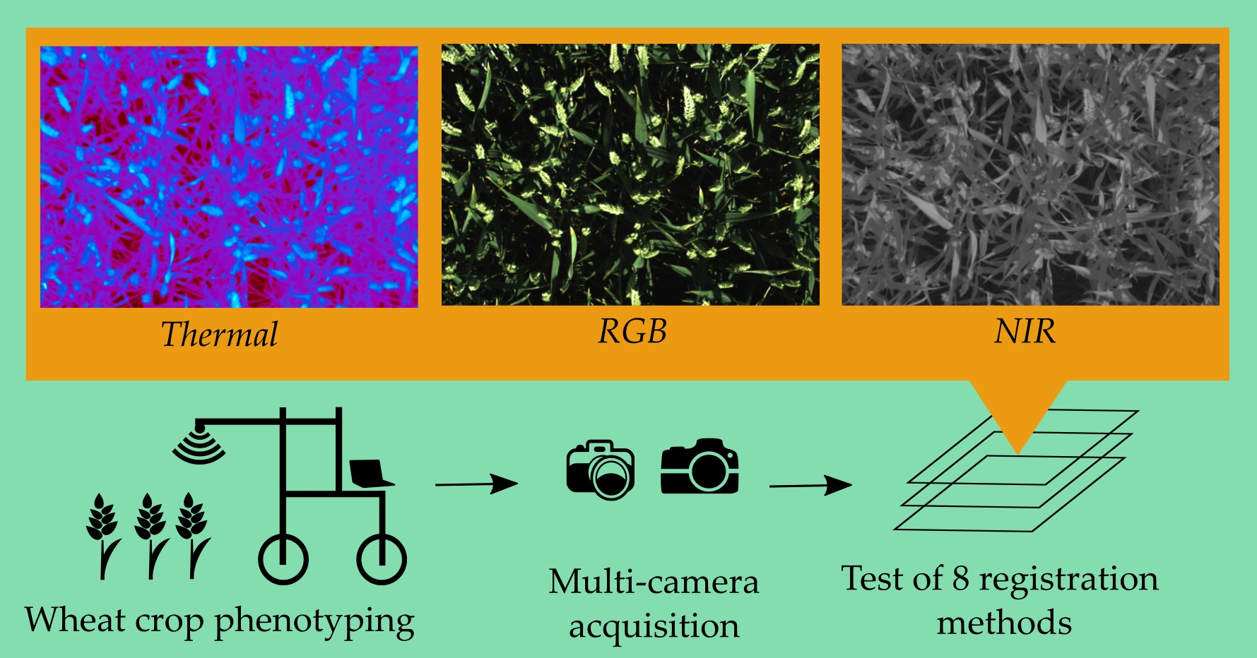
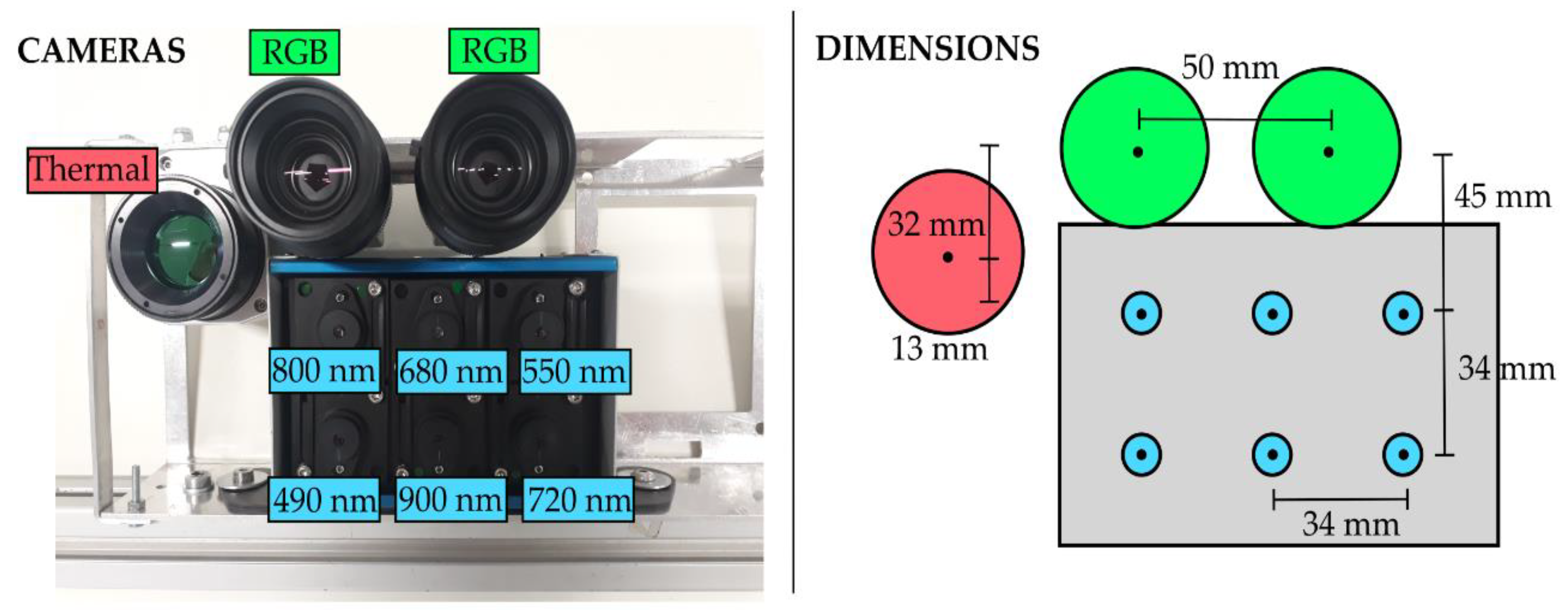
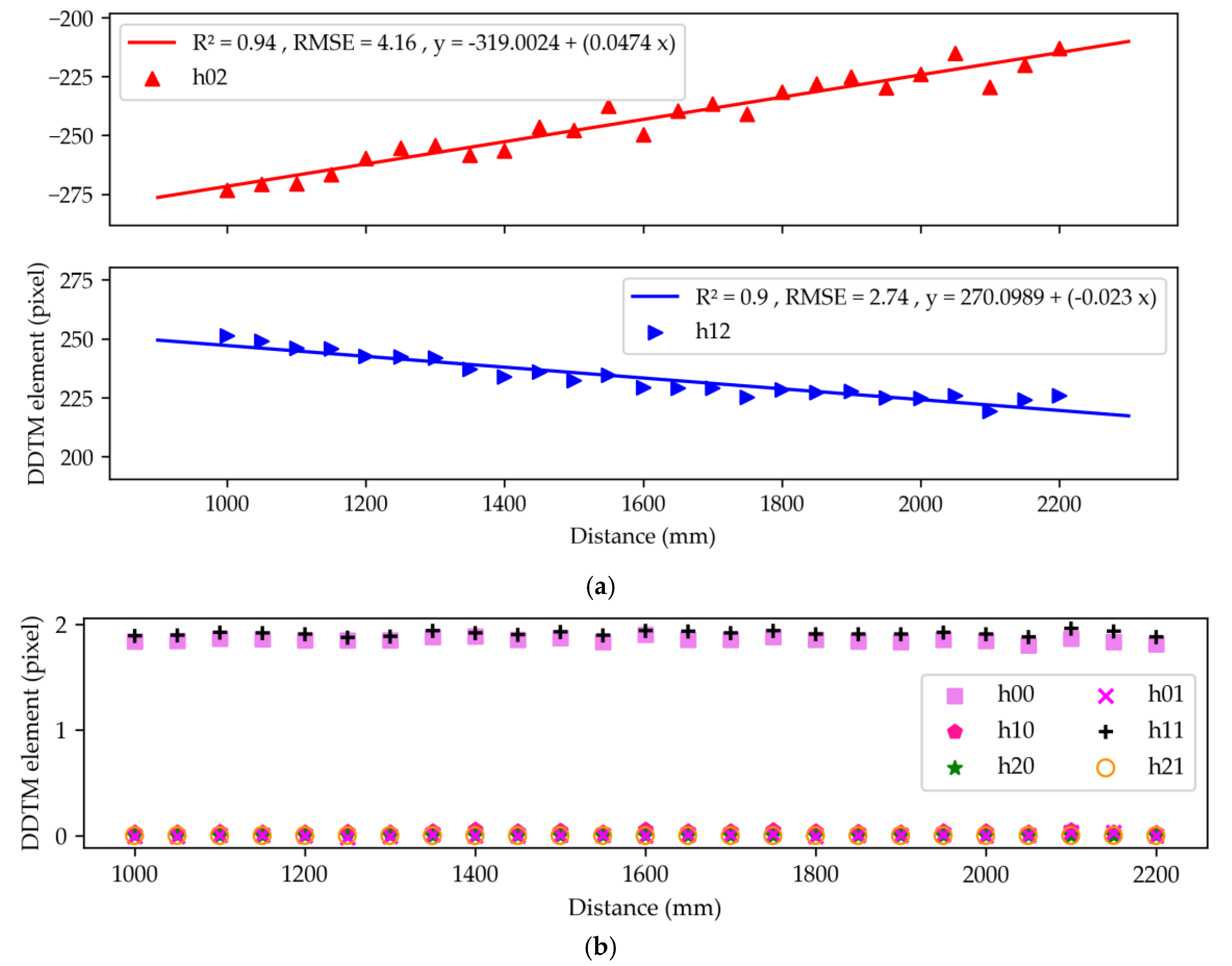
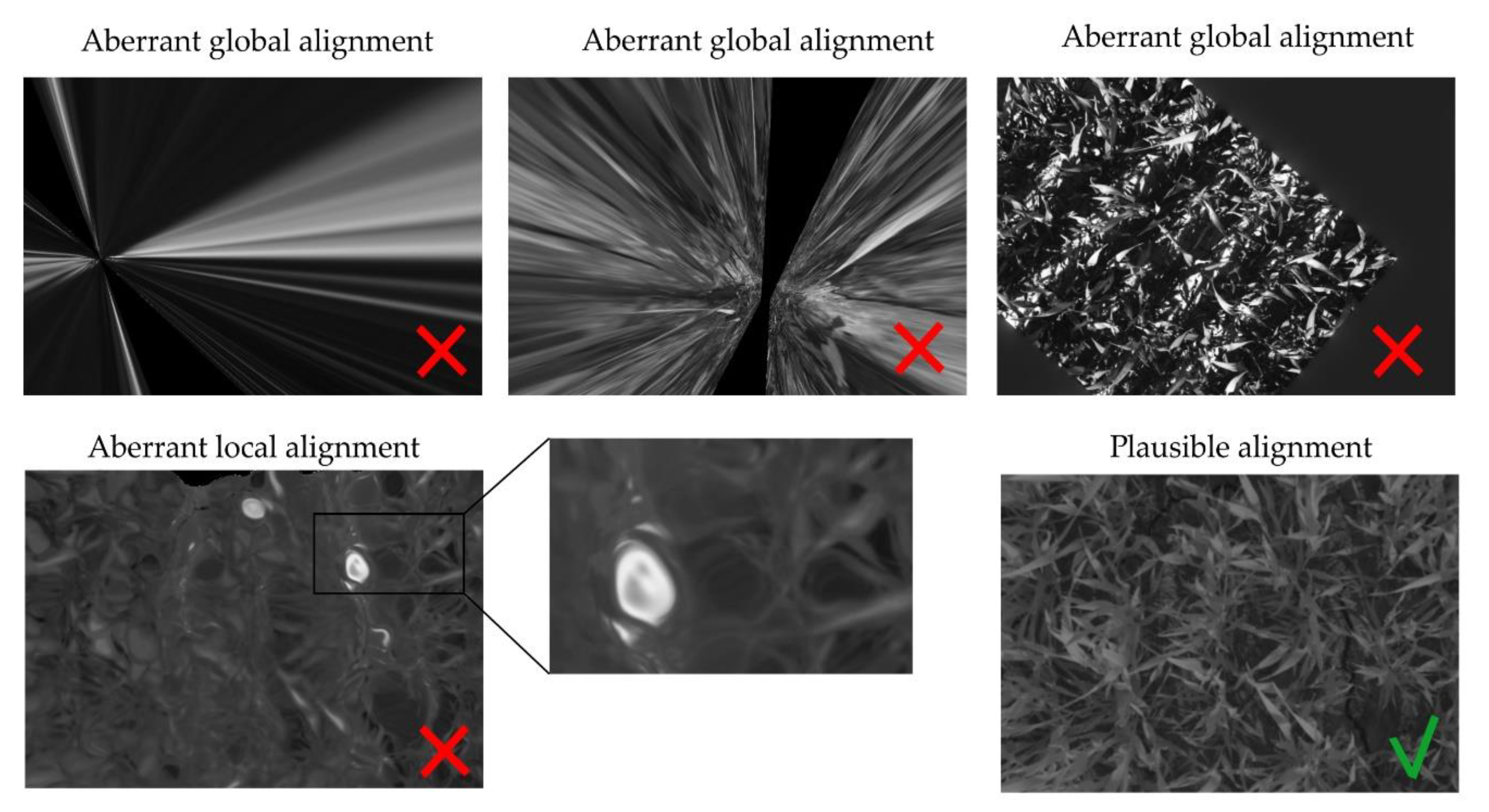
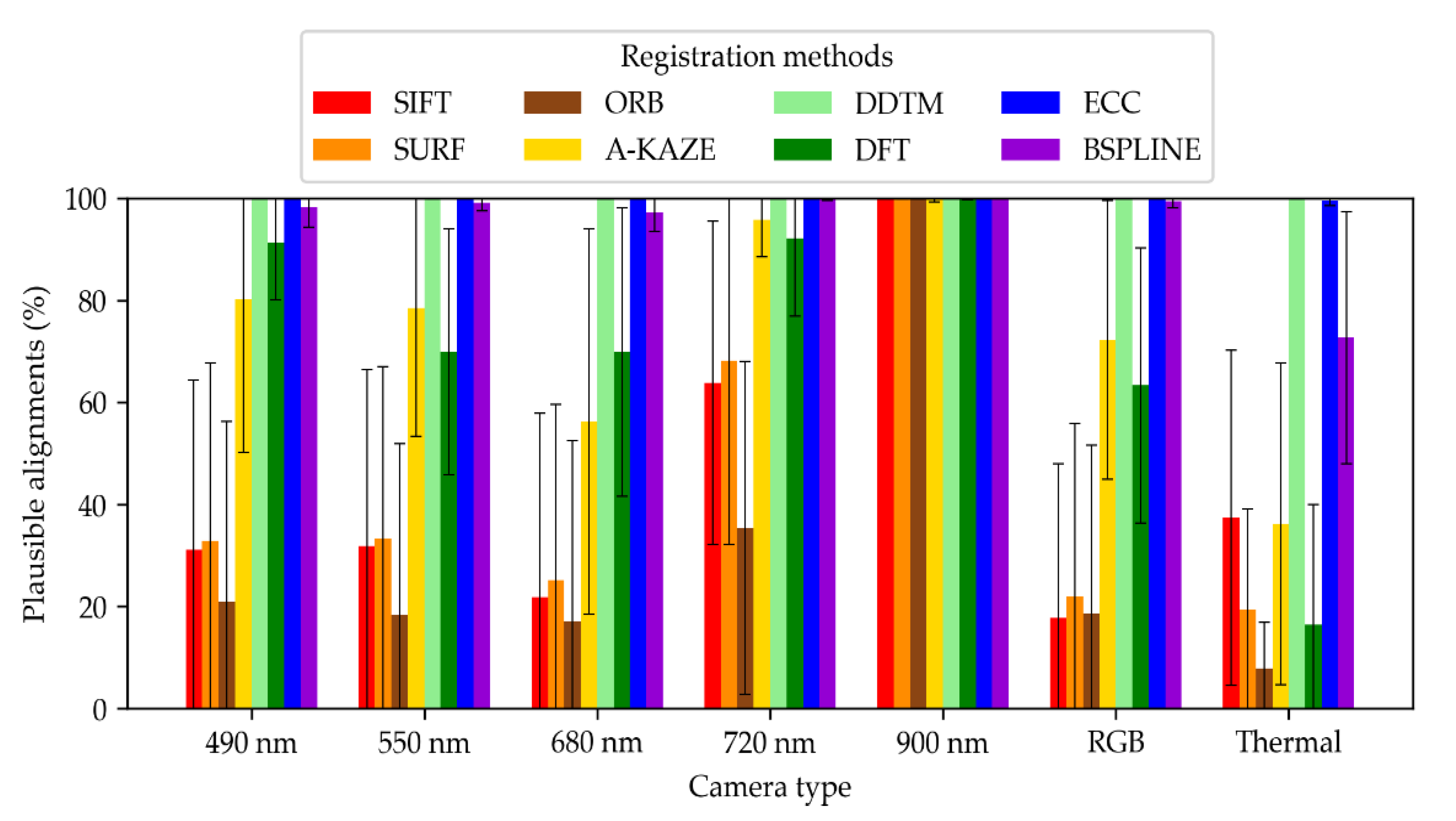
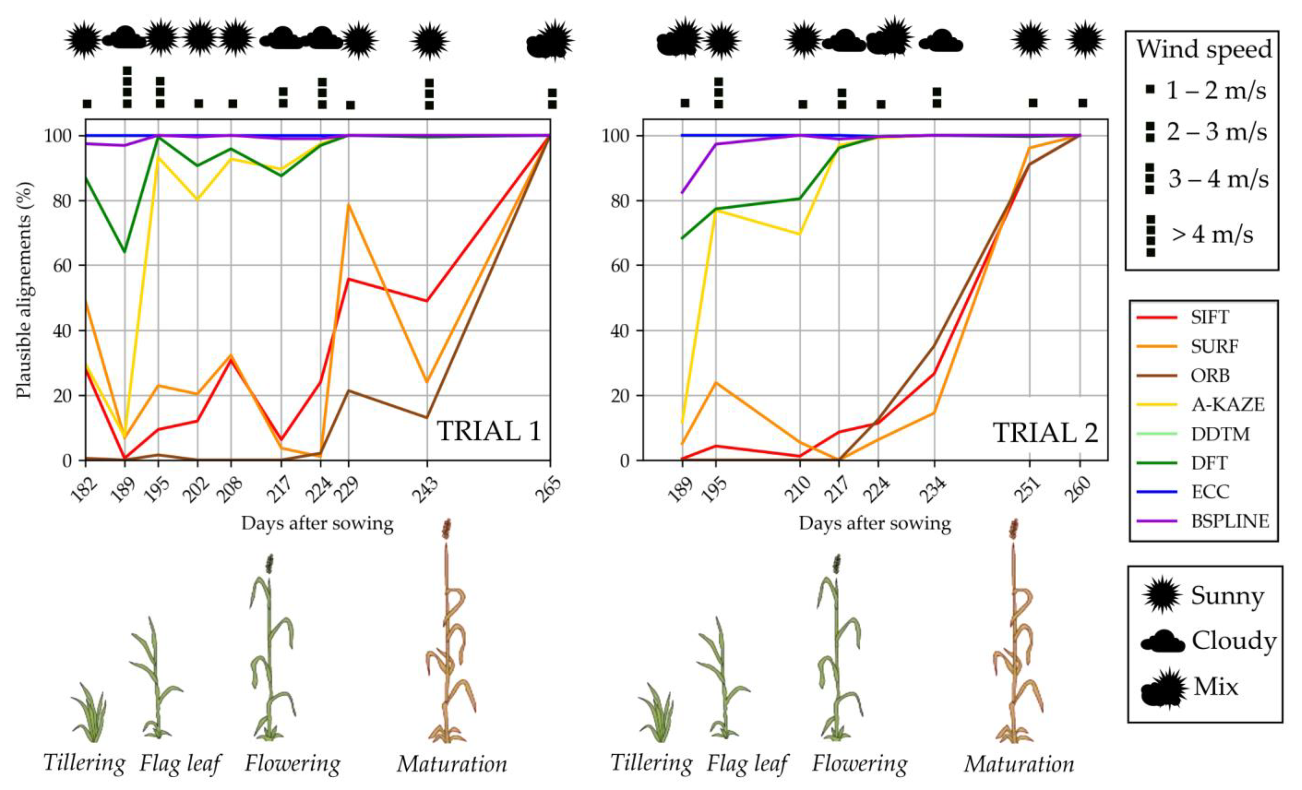
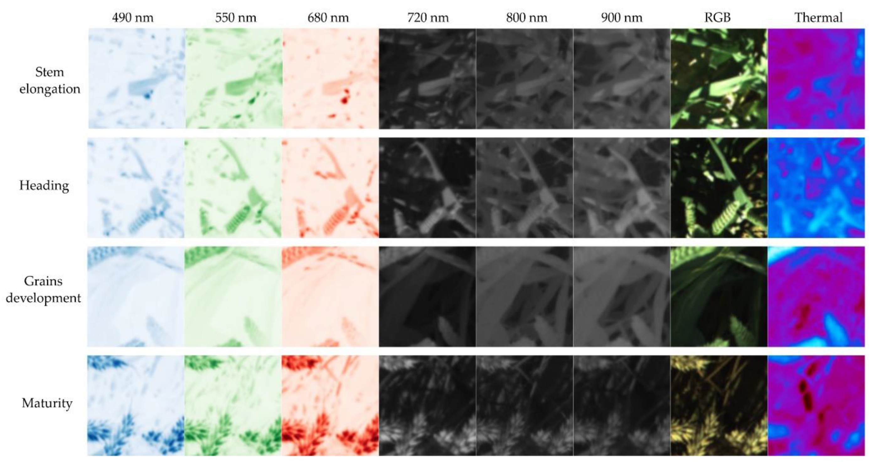
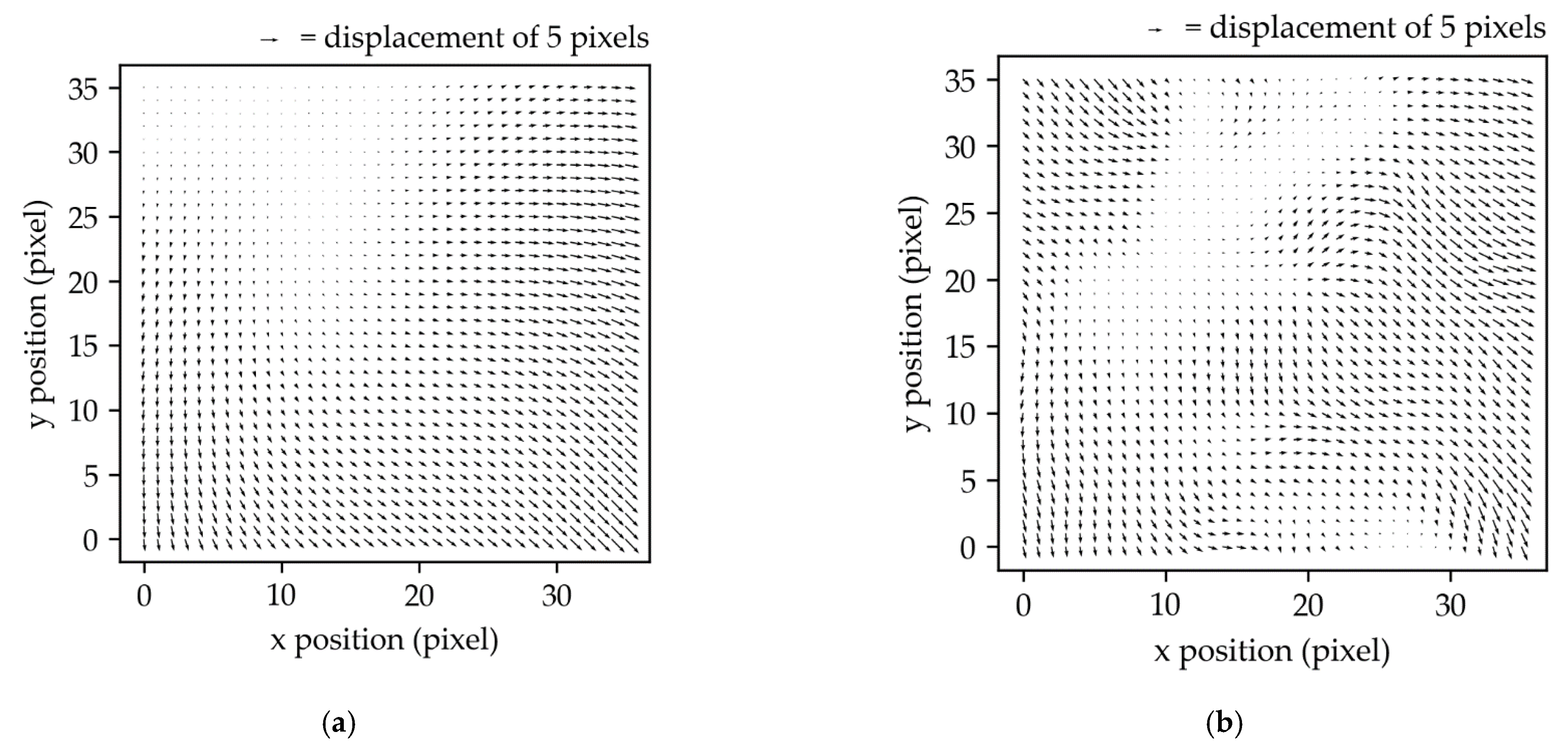
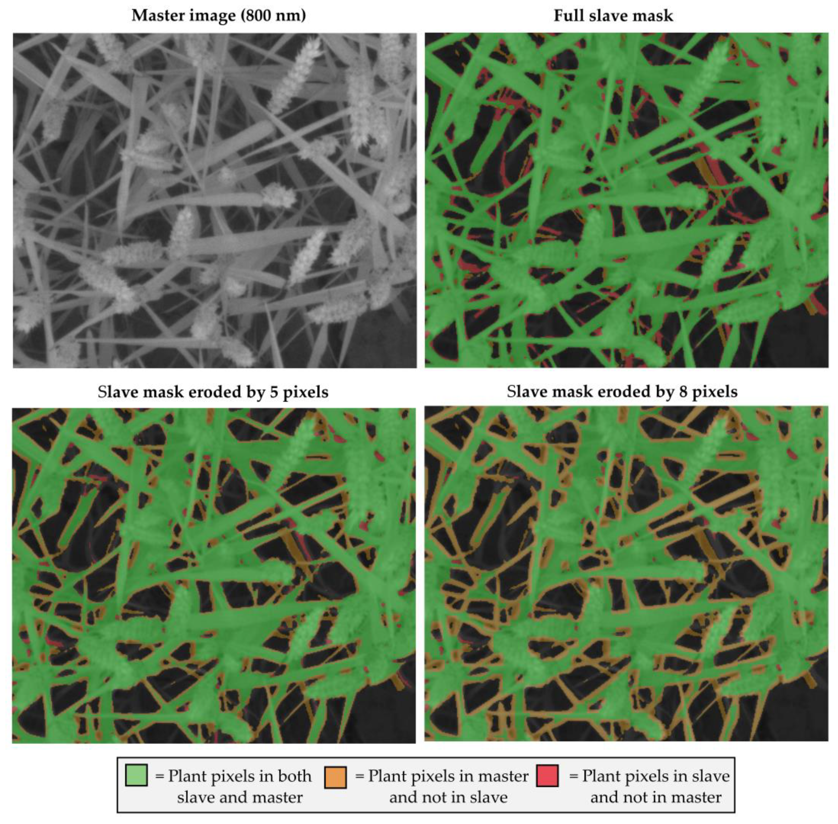
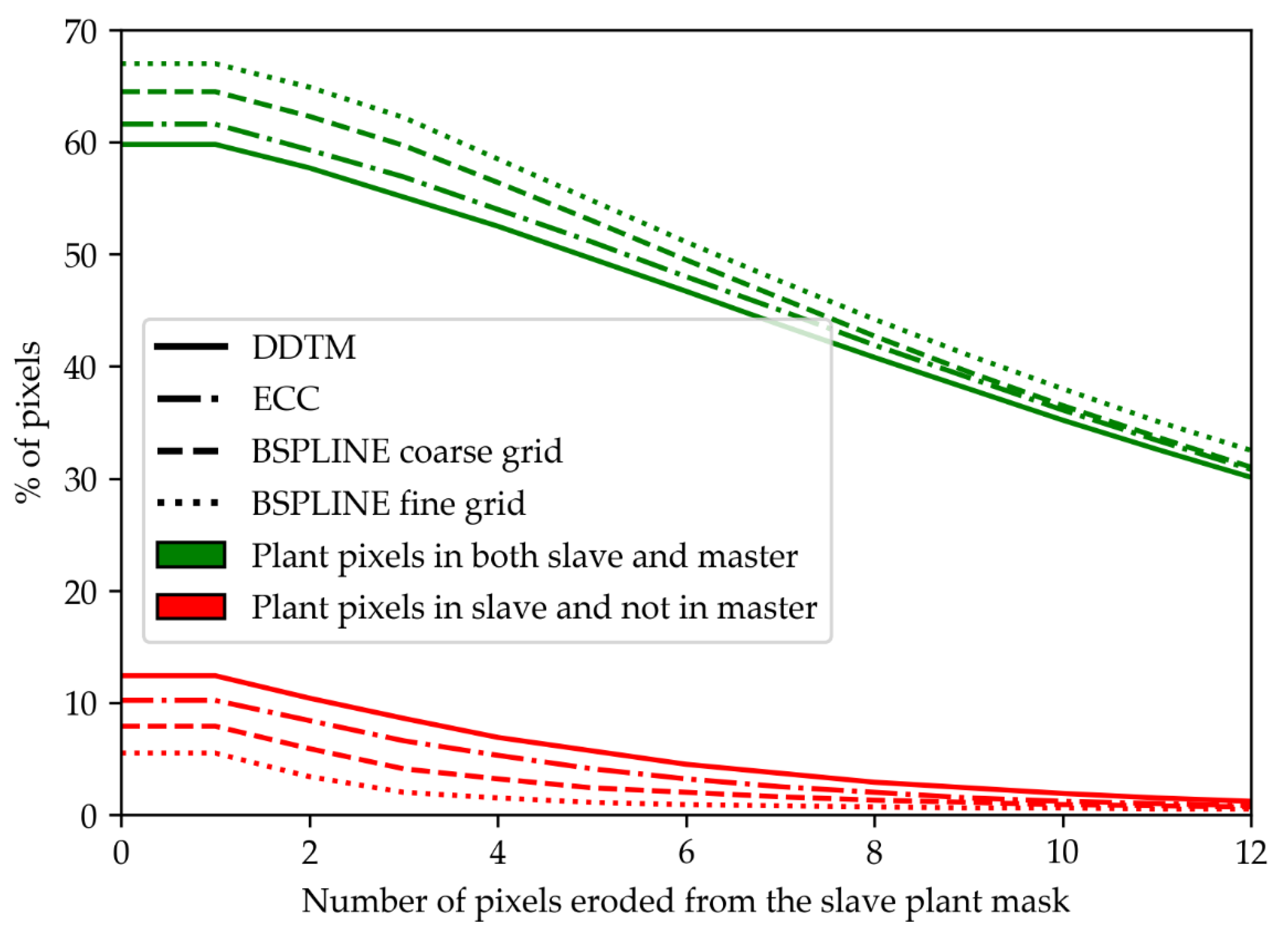
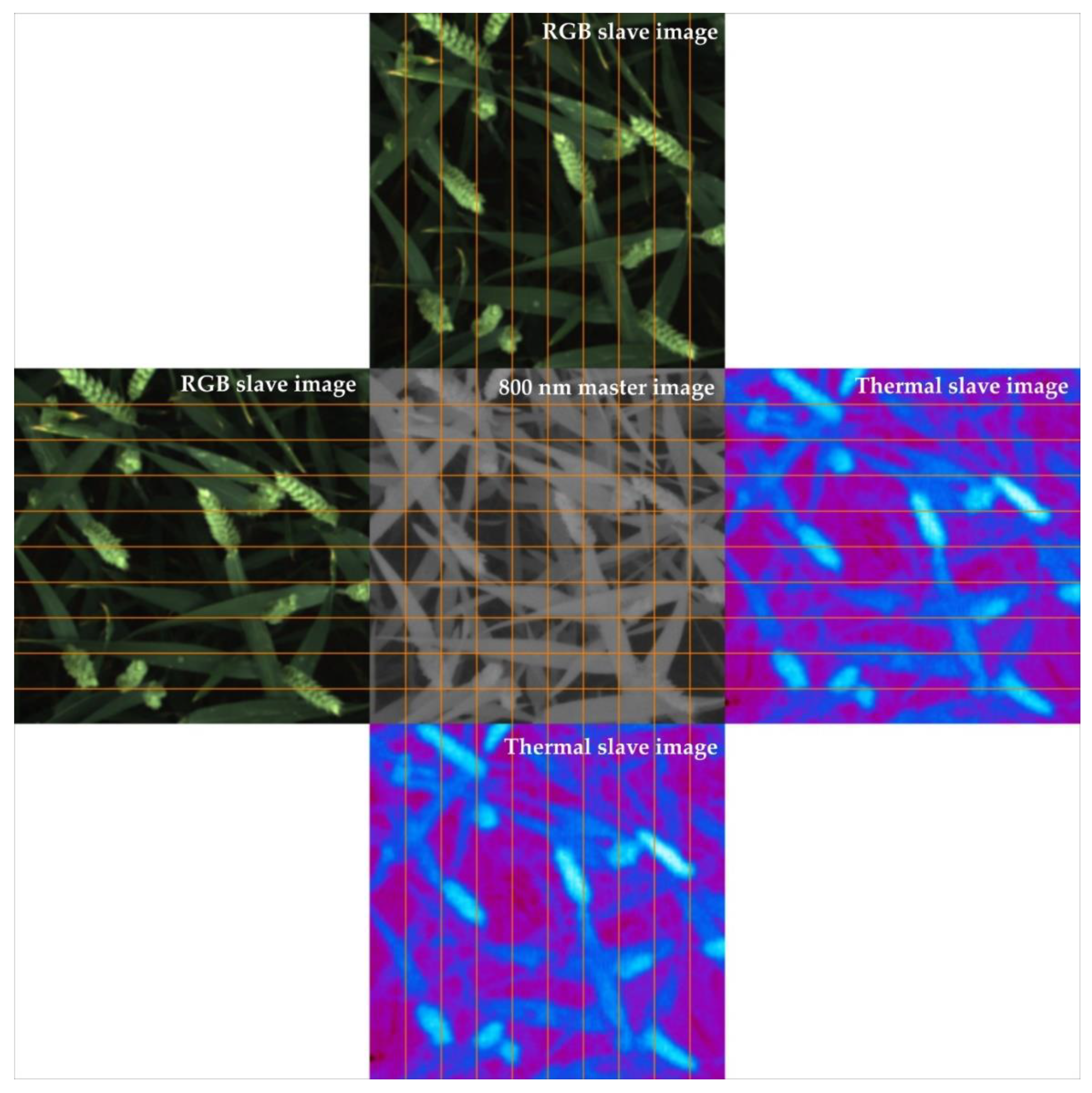
Table 1.
Summary of registration methods tested in this study.
| Method | Matching | Transformation | Resampling | Library | Origin |
|---|---|---|---|---|---|
| SIFT | Features-based | Homography | Bilinear | OpenCV [35] | [38] |
| SURF | Features-based | Homography | Bilinear | OpenCV | [39] |
| ORB | Features-based | Homography | Bilinear | OpenCV | [40] |
| A-KAZE | Features-based | Homography | Bilinear | OpenCV | [41] |
| DDTM | / | Homography | Bilinear | / | [33] |
| DFT | Area-based | Similarity | Bilinear | imreg_dft | [42] |
| ECC | Area-based | Homography | Bilinear | OpenCV | [43] |
| B-SPLINE | Area-based | B-spline | Bilinear | Elastix [26] | [44] |
Table 2.
Comparison of the registration methods based on three criteria: the average computation time to register one image of all cameras, the control points error and the plant mask error. Errors are averaged for dates before and after ears emergence. For the RGB images, some methods were discarded (NA values) because they did not yield a plausible alignment for all the test images.
| Method | Average Time (s) | Control Points Error (mm) | Plant Mask Error (%) | ||||
|---|---|---|---|---|---|---|---|
 | 900 nm | RGB | 900 nm | RGB | 900 nm | 900 nm | |
| SIFT | 4.0 | 3.7 | NA | 3.4 | NA | 9.7 | 9.7 |
| SURF | 6.2 | 3.6 | NA | 3.4 | NA | 9.5 | 9.5 |
| ORB | 1.0 | 5.5 | NA | 3.6 | NA | 10.6 | 10.3 |
| A-KAZE | 2.7 | 3.4 | NA | 3.7 | NA | 10.1 | 9.7 |
| DDTM | 2.6 | 5.2 | NA | 4.2 | NA | 11.7 | 10.5 |
| DFT | 41.3 | 3.9 | NA | 4.1 | NA | 9.7 | 9.8 |
| ECC | 21.9 | 3.2 | 3.0 | 3.0 | 3.0 | 9.8 | 9.7 |
| B-SPLINE | 176.7 | 1.9 | 2.0 | 2.0 | 1.6 | 7.0 | 6.5 |
Table 3.
Proposed registration–fusion strategies. Each row presents a strategy.
| Strategy Name | Registration | Plant Mask Erosion | Intensity Averaging | Computation Time | Scope |
|---|---|---|---|---|---|
| REAL-TIME | DDTM | Wide | Wide window | Instantaneous | Suitable for multimodal images |
| FAST | DDTM + ECC | Medium | Medium window | Moderated | Suitable for multimodal images |
| ACCURATE | DDTM + B-SPLINE (coarse grid) | Medium | Small window | Slow | Not suitable for thermal images (if the master is NIR) |
| HIGHLY ACCURATE | DDTM + B-SPLINE (fine grid) | Tiny or none | None | Extremely slow | Limited to mono-modal images |
Publisher’s Note: MDPI stays neutral with regard to jurisdictional claims in published maps and institutional affiliations. |
© 2021 by the authors. Licensee MDPI, Basel, Switzerland. This article is an open access article distributed under the terms and conditions of the Creative Commons Attribution (CC BY) license (https://creativecommons.org/licenses/by/4.0/).
Share and Cite
MDPI and ACS Style
Dandrifosse, S.; Carlier, A.; Dumont, B.; Mercatoris, B. Registration and Fusion of Close-Range Multimodal Wheat Images in Field Conditions. Remote Sens. 2021, 13, 1380. https://0-doi-org.brum.beds.ac.uk/10.3390/rs13071380
AMA Style
Dandrifosse S, Carlier A, Dumont B, Mercatoris B. Registration and Fusion of Close-Range Multimodal Wheat Images in Field Conditions. Remote Sensing. 2021; 13(7):1380. https://0-doi-org.brum.beds.ac.uk/10.3390/rs13071380
Chicago/Turabian StyleDandrifosse, Sébastien, Alexis Carlier, Benjamin Dumont, and Benoît Mercatoris. 2021. "Registration and Fusion of Close-Range Multimodal Wheat Images in Field Conditions" Remote Sensing 13, no. 7: 1380. https://0-doi-org.brum.beds.ac.uk/10.3390/rs13071380
Note that from the first issue of 2016, this journal uses article numbers instead of page numbers. See further details here.