
Responses of Summer Upwelling to Recent Climate Changes in the Taiwan Strait


State Key Laboratory of Marine Environmental Science, Key Laboratory of Underwater Acoustic Communication and Marine Information Technology Ministry of Education, College of Ocean and Earth Sciences, Xiamen University, Xiamen 361102, China
Remote Sens. 2021, 13(7), 1386; https://doi.org/10.3390/rs13071386
Submission received: 5 March 2021
/
Revised: 24 March 2021
/
Accepted: 1 April 2021
/
Published: 3 April 2021
Abstract
:The response of a summer upwelling system to recent climate change in the Taiwan Strait has been investigated using a time series of sea surface temperature and wind data over the period 1982–2019. Our results revealed that summer upwelling intensities of the Taiwan Strait decreased with a nonlinear fluctuation over the past four decades. The average upwelling intensity after 2000 was 35% lower than that before 2000. The long-term changes in upwelling intensities show strong correlations with offshore Ekman transport, which experienced a decreasing trend after 2000. Unlike the delay effect of canonical ENSO events on changes in summer upwelling, ENSO Modoki events had a significant negative influence on upwelling intensity. Strong El Niño Modoki events were not favorable for the development of upwelling. This study also suggested that decreased upwelling could not slow down the warming rate of the sea surface temperature and would probably cause the decline of chlorophyll a in the coastal upwelling system of the Taiwan Strait. These results will contribute to a better understanding of the dynamic process of summer upwelling in the Taiwan Strait, and provide a sound scientific basis for evaluating future trends in coastal upwelling and their potential ecological effects.

1. Introduction
Coastal upwelling is an important component of circulation in the shelf marginal sea. It develops when prevailing alongshore winds force offshore Ekman transport of surface waters, which brings cold, nutrient-rich water up to the euphotic layer, leading to high concentrations of chlorophyll [1,2]. Understanding how coastal upwelling systems respond to climate change has become an area of intensive research in recent years because of the importance of upwelling to marine fisheries, biodiversity, and the carbon cycle. Many studies on eastern boundary upwelling systems [3,4,5] demonstrate an enhancement trend in upwelling intensity under modern climate change. Meanwhile, weakening upwelling trends are observed in other regions, such as the NW Iberian Peninsula coastal upwelling [6], which is contrary to the hypothesis of Bakun [3]. These studies have revealed that upwelling trends depend heavily on a time series of different seasons, lengths, and sources, as well as the location analyzed [7,8,9,10]. However, little research has been conducted on the effect of global warming on the western boundary upwelling during the Asian summer monsoon region [11]. This topic is especially important due to the already stressed condition of the upwelling ecosystem in this region due to human activities such as overfishing and pollution.
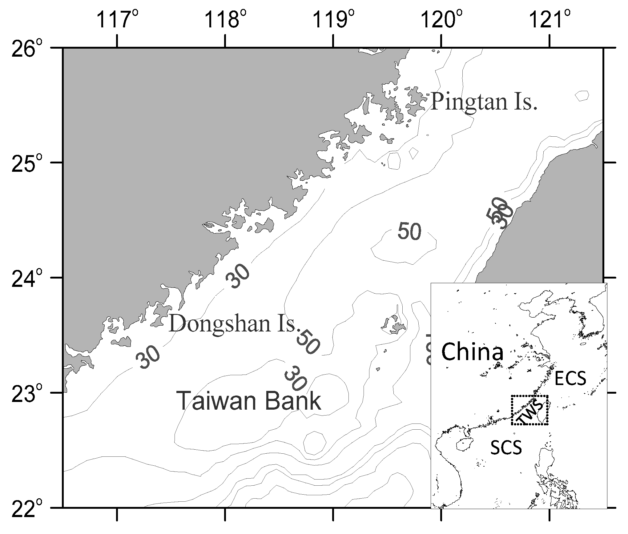
The Taiwan Strait (TWS) is an important channel connecting the South China Sea and the East China Sea. It is characterized by rough bottom topography (Figure 1) and a complicated current system. The circulation of the TWS is controlled mainly by the East Asia monsoon [12]. Strong northeasterly winds prevail in the winter, and weak southwesterly winds dominate in the summer [13]. During the summer monsoon, the circulation of TWS is controlled by the warm SCS water. At this time, upwelling events are generally observed along the coast of the western TWS and around the Taiwan Bank [14,15]. Beginning in the 1980s, extensive studies have been conducted to examine the location, variability, control mechanisms, and ecological response of upwelling in the TWS based on in situ measurements, satellite observations, or numerical modelling [16,17,18,19,20,21,22]. The characteristics of several dominant upwelling subregions such as the Pingtan upwelling zone (PTU), the Dongshan Upwelling zone (DSU), and the Taiwan Bank upwelling zone (TBU) have also been investigated. These studies have demonstrated that these upwellings are principally induced by the southwesterly monsoon and the ascending movement of the northward, near-bottom current along the bottom topography [14]. Moreover, the size or intensity of upwelling-related low temperature zones have substantial variability, and that variation over short-term or interannual time scales is significantly controlled by alongshore wind stress [23,24,25,26]. Furthermore, long-term changes in sea surface temperature have been investigated using long-term time series of satellite-derived sea surface temperature datasets [27,28]. However, long-term changes in summer upwelling in the TWS have not been fully studied and understood. Detailed information on the influence of upwelling on sea surface temperature and chlorophyll a is particularly lacking.
As the dominant modes of earth climate indices, ENSO (El Niño Southern Oscillation) events play an important role in the hydrodynamics and ecosystems of many upwelling systems [29,30]. Studies have shown that there are two types of ENSO events. One is the canonical El Niño event, in which anomalous warming occurs in the eastern equatorial Pacific Ocean. Its variation can be represented by the normalized Multivariate El Niño/Southern Oscillation Index (MEI) [31]. Significantly positive (negative) values of the MEI indicate El Niño (La Niña) conditions. Another variation is El Niño Modoki, characterized by a warm SST anomaly in the central equatorial Pacific. The normalized El Niño Modoki index (EMI) is used to distinguish the changes of El Niño Modoki events [32]. The more positive the EMI, the stronger the El Niño Modoki. Thus far, research on the hydrodynamics and ecosystems of the Taiwan Strait by canonical ENSO events has received a lot of attention [28,33,34]. These studies suggest that the delayed ENSO effect is a major mechanism for the interannual variability of hydrodynamics in the Taiwan Strait. However, little research has been conducted on the impact of ENSO Modoki events on changes in the ecological environment of the TWS upwelling system.
In this study, we utilize available time series of sea surface temperature (SST), wind, and chlorophyll a to investigate the long-term changes in upwelling intensity in the Taiwan Strait. The questions addressed in this research include: How has the upwelling system of the TWS responded to climate change over the past decades? Are there any differences in the trends of upwelling intensity for the main three upwelling subregions including PTU, DSU, and TBU? Do ENSO Modoki events have any effects on upwelling? What are the influences of long-term changes in upwelling intensity on sea surface temperature and chlorophyll a? The answers to these questions are very important to our understanding of the dynamic process of upwelling as well as to the management and protection of fishery resources in the TWS in the context of global change.
2. Materials and Methods
2.1. SST Data
The AVHRR Pathfinder Version 5.3 (PFV5.3) sea surface temperature (SST) data from 1982 to 2019 were obtained from the US National Oceanographic Data Center and GHRSST (http://pathfinder.nodc.noaa.gov, accessed on 5 March 2021). The PFV5.3 SST data are an updated version of the Pathfinder Versions 5.0 and 5.1 collection described in Saha et al. [35]. The PFV5.3 SST dataset is a collection of global, twice daily (day and night) 4-km sea surface temperature data. The validation of PFSST with a drifting buoy indicated that it agreed well with in situ observations in the study region, with a mean bias ± standard deviation (STD) of −0.33 °C ± 0.79 °C [36]. The PFSST dataset has been widely used for global or regional ocean and climate studies [37].
In this study, the night daily SST data were used to calculate the monthly SST through arithmetic averaging. Next the summer average SST was calculated from the monthly data for June, July, and August. Anomalies in SST (SSTA) were calculated as the deviation from the summer climatological means between 1982 and 2019.
2.2. Characterization of Upwelling Based on SST and Wind
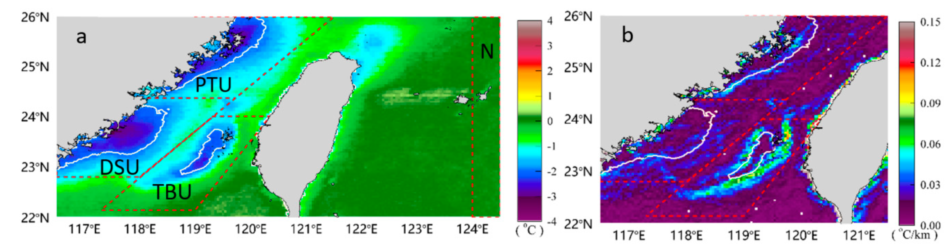
In order better to characterize changes in the upwelling zones of TWS, the difference in SST (ΔSST) between the TWS and non-upwelling zone were calculated. The ΔSST calculation was performed by subtracting the average SST of the non-upwelling zone from the SST of the TWS. The TWS refers to the water between 22–26°N and 116.5–121.5°E, as shown in Figure 1. The non-upwelling zone refers to the offshore water between 22–26°N and 124–124.5°E (Figure 2a). The subregions DSU, PTU, and TBU are also illustrated in Figure 2a.
Upwelling intensity (R) is defined following the methods from Kuo et al. [38] and Shang et al. [24]:
where Ai is the area of the upwelling region, ΔTi is ΔSST, that is, the decrease in SST relative to the average SST of non-upwelling water, and di refers to the upwelling depth. Pond and Pickard [39] estimated di by
where Vi is the wind speed and φi is the latitude of the upwelling zones. They are represented as the average wind speed and latitude of the PTU, DSU, and TBU zones. The ΔTi Ai in the three upwelling zones was calculated pixel by pixel on waters colder than non-upwelling water by a threshold value. For the three upwelling subzones, the threshold value was chosen as 2.0 °C. Figure 2b indicates that the SST difference of the −2.0 °C contour was consistent with the positions of the fronts between cold upwelling water and warm water.
2.3. Wind Data and Ekman Transport
The monthly European Centre for Medium-Range Weather Forecasts (ECMWF) ERA5 global 0.25° × 0.25° reanalysis dataset was downloaded from the Asia-Pacific Data Research center (http://apdrc.soest.hawaii.edu/, accessed on 5 March 2021). ERA5 is the fifth generation ECMWF reanalysis for the global climate and weather, covering from 1979 to 2019. Two variables, the 10-m u wind component (Wx) and v wind component (Wy) were used in this study.
The zonal and meridional components of wind stress (τx,τy) were calculated from the wind speed (W = (Wx,Wy)) according to Zhang et al. [28], as follows:
where ρa is the air density (1.22 kg m−3) and Cd is the dimensionless drag coefficient from Trenberth et al. [40]:
The Ekman transport factors Qx and Qy were calculated as follows:
where ρw is the density of sea water (1025 kg m−3), f is the local Coriolis parameter (defined as twice the component of the angular velocity of the earth, Ω, at latitude θ, or f = 2Ω sin(θ), where Ω = 7.292 × 10⁻⁵ s−1).
The cross-shore Ekman transport (Qcross), which also refers to upwelling index, is defined as the Ekman transport component in the direction perpendicular to the shoreline [41]. It was calculated as follows:
where φ is the mean angle between the shoreline and the equator. Positive values of Qcross indicate upwelling-favorable conditions, while negative values of Qcross indicate downwelling-favorable conditions [41].
2.4. Other Data
Monthly level-3 chlorophyll a (Chl) data from the Moderate Resolution Imaging Spectroradiometer (MODIS) aboard the Aqua satellite (retrieved with the MODIS OC3M standard algorithm) were obtained from the Ocean Biology Processing Group (OBPG) at NASA’s Goddard Space Flight Center (http://oceancolor.gsfc.nasa.gov, accessed on 5 March 2021). The temporal coverage was between 2003 and 2019, and the spatial resolution was 4 km.
The numerical values of the monthly Multivariate ENSO (El Niño/Southern Oscillation) Index (MEI), and El Niño Modoki index (EMI) were downloaded from Earth System Research Laboratory’s Physical Sciences Division (PSD) of National Oceanic and Atmospheric Administration (https://www.esrl.noaa.gov/psd/enso/mei/, accessed on 5 March 2021), and the Japan Agency for Marine-Earth Science and Technology (http://www.jamstec.go.jp/frsgc/research/d1/iod/modoki_home.html.en, accessed on 5 March 2021), respectively.
2.5. Statistical Method
The Locally Weighted Scatterplot Smoother (LOWESS or LOESS) method was used in this study to detect non-linear trends. In some cases, linear regression cannot clarify the relationships between variables and cannot detect the trend of a data series. To overcome such limitations and provide qualitative results, the LOWESS method is found to be an effective regression approach for long-term environmental data with non-linear trends [42,43,44]. As a non-parametric smoothing procedure and locally weighted average model, the LOWESS method produces a smooth line through a scatterplot, which helps to understand the trends of variables [43]. Detailed information about this method can be found in studies by Cleveland [43] and Lee et al. [42].
3. Results
The temporal variation of upwelling intensity (R) calculated based on SST and wind data in the three subregions of PTU, DSU, and TBU are shown in Figure 3. The variability of R in the three subregions is almost the same. There were no significant differences between R of any two subregions using the independent t–test.
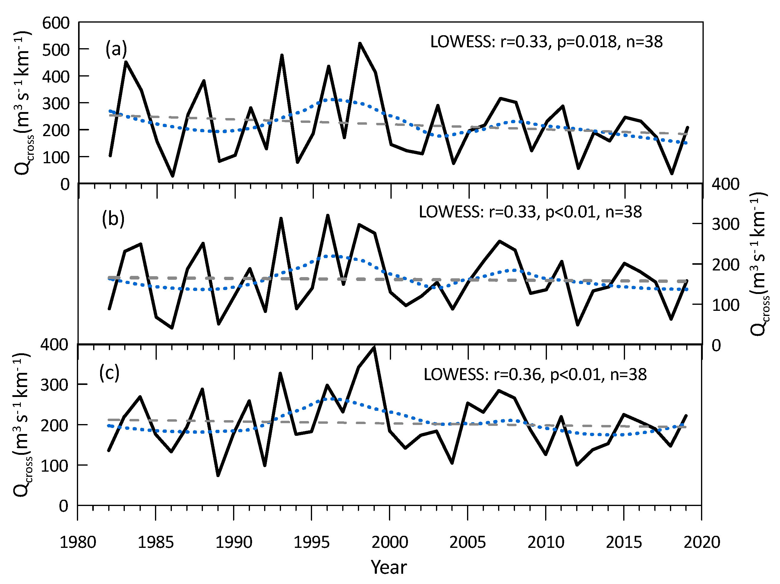
Statistical results show that the upwelling intensity decreased every year from 1982 to 2019 (Figure 3), but the linear trend of R did not pass the significance test. The LOWESS was then adopted to detect the non-linear trend of R over time. The regression fit lines from LOWESS are overlaid on Figure 3, as shown by the dotted lines. All of these regression fit lines pass the significance test (p < 0.05). Figure 3 shows that the changes in R varied with a non-linear fluctuation over the period 1982–2019. The R increased slightly before 1996 and during 2003–2007, and decreased from 1996 to 2003 and after 2007.
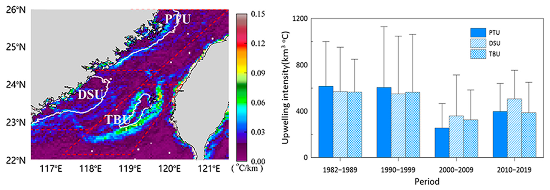
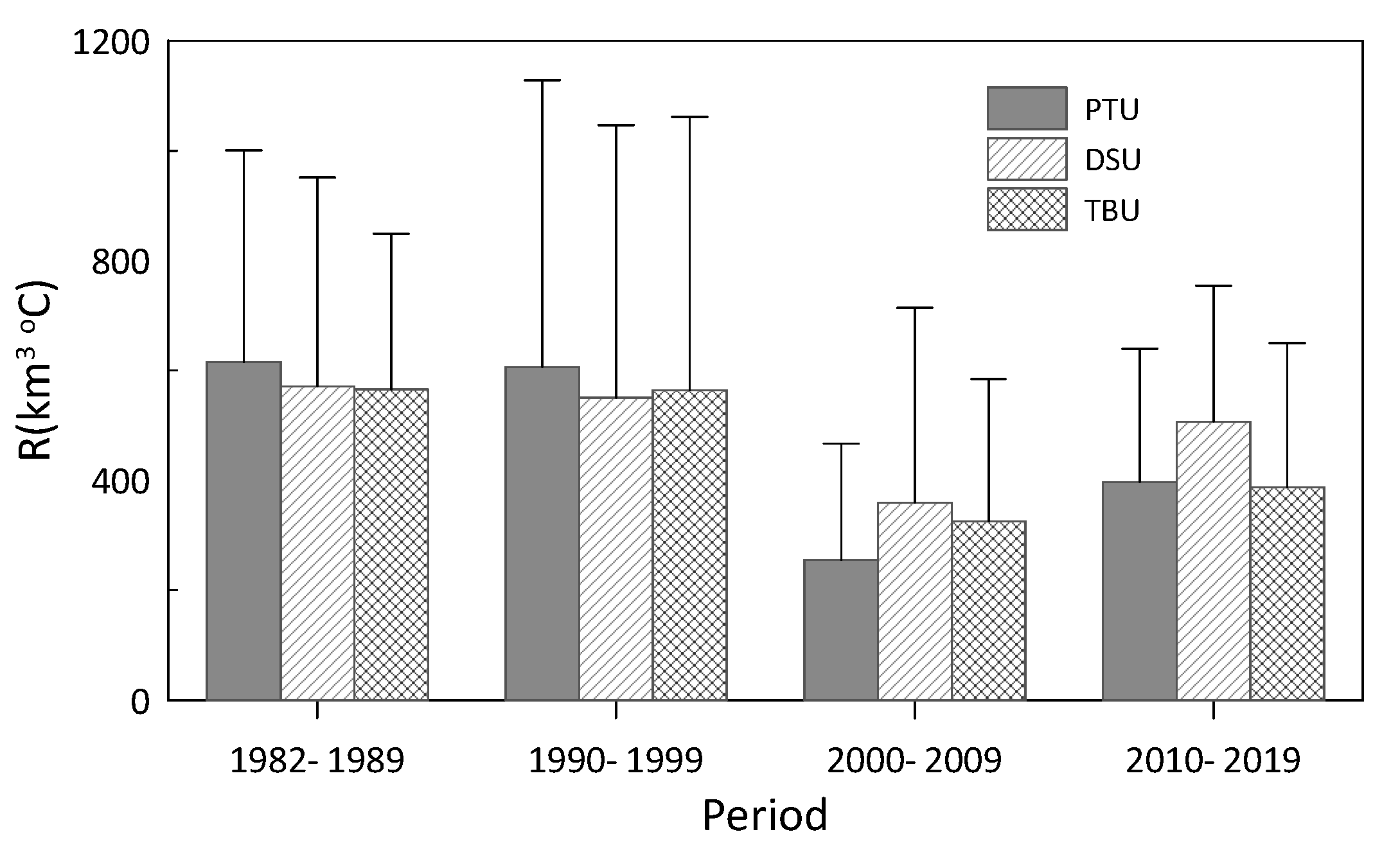
Four different periods during the 1980s (1982–1989), 1990s (1990–1999), 2000s (2000–2009), and 2010s (2010–2019) were chosen to further investigate variation in upwelling intensity (Figure 4). Figure 4 indicates that the upwelling intensity in the three sub regions was the lowest in the 2000s, and the R decreased significantly from the 1990s to 2000s. From the 2000s to the 2010s, the R of the three subregions increased. However, the average value of R in the 2010s was much smaller than the R before 2000. We roughly separated the time series data into two periods separated by the year 2000. Table 1 shows the statistical results in changes of R before 2000 and after 2000. On average, the upwelling intensity (R) after 2000 was 35% less than that before 2000. Among the three subregions, the decrease of R in PTU is the most obvious, with R decreasing by 46%.
Similar variations were also found in the cross-shore Ekman transport (Qcross, Figure 5) using linear and LOWESS method. During the study period, there was a slight increase in Qcross before 1996, then a decrease during 1996–2003. After 2003, the Qcross increased during 2003–2007, and slightly decreased after 2007. The average value of Qcross after 2000 was much lower than before 2000 (Table 1), especially for the PTU.
4. Discussion
4.1. Changes of Upwelling Intensity
Figure 3 and Figure 4, and Table 1, show that from 1982 to 2019, the upwelling intensity in the Taiwan Strait varied with a nonlinear fluctuation. Although the linear trend of decreasing R did not pass the significance test, the average upwelling intensity after 2000 was 35% lower than that before 2000 (Table 1). Similar upwelling weakening was found along the Hainan and Zhejiang coast of the China Sea [45,46]. Liu et al. (2013) demonstrated that since the 1960s, the upwelling intensity in the northern South China Sea has decreased. Other upwelling systems, such as the Iberian coastal upwelling [47] and low latitude Canary upwelling system [7], are reported to have a weakening in upwelling intensity. The decreasing upwelling trend seen in these areas is quite different from the north eastern boundary upwelling systems, which have a strengthening of upwelling [2,48].
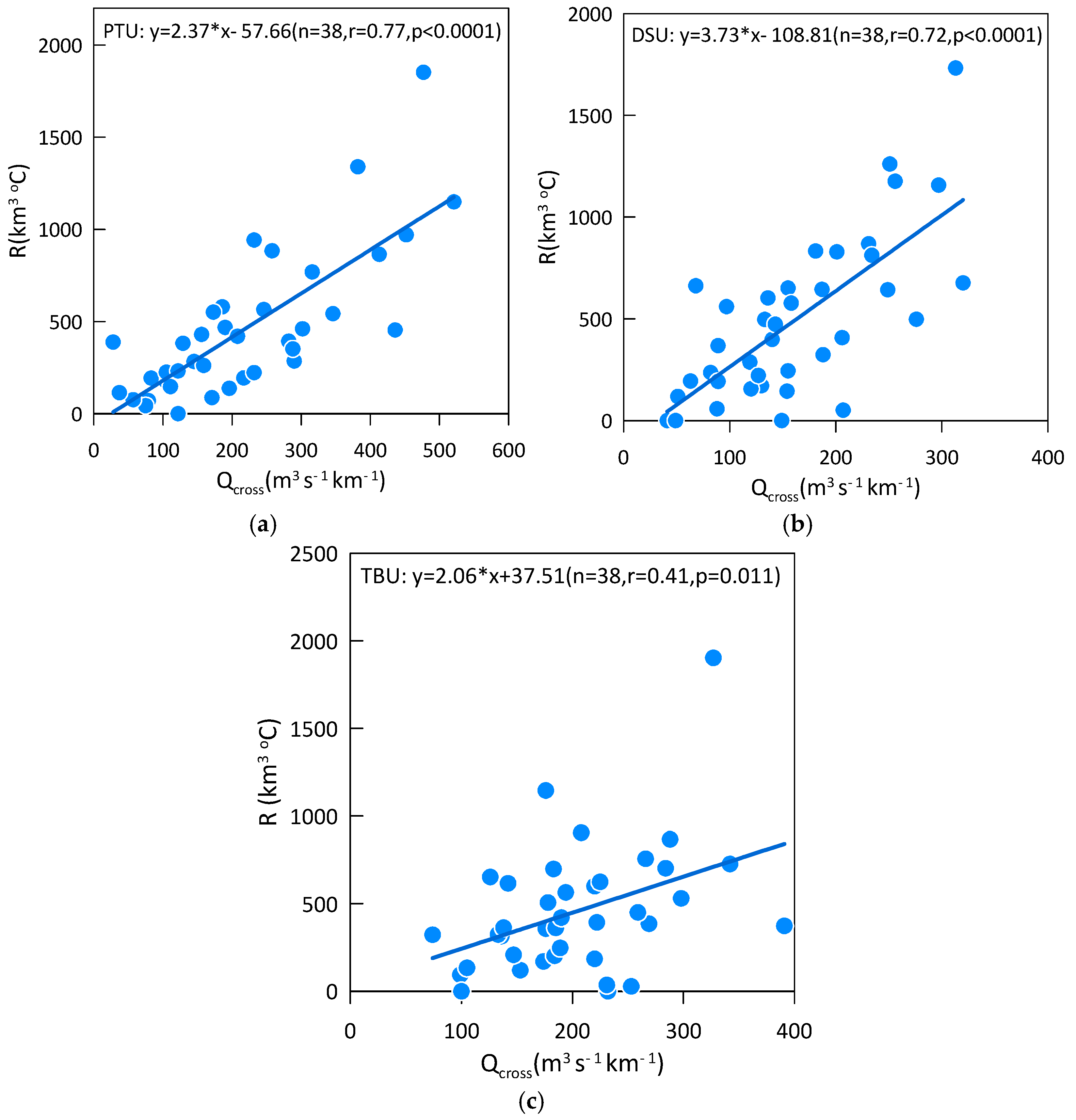
Figure 3 and Figure 5 indicate that the changes in upwelling intensity of PTU, DSU, and TBU are consistent with changes in cross-shore Ekman transport. Further statistical correlations (Figure 6) show that there are significant correlation between R and Qcross in the three subregions (p ≤ 0.05), especially in the PTU and DSU, which suggests that Ekman transport is the dominant mechanism pumping cold water upward to the surface in the TWS. Several studies have also demonstrated that short-term or interannual variability of coastal upwelling is closely correlated with changes in alongshore wind stress in the TWS [23,26].
In recent decades, the East Asian summer monsoon has been observed to weaken [49,50]. Figure 5 and Table 1 reveal that the upwelling-favorable Ekman transport of the three subregions in the TWS decreased over the last 40 years. Therefore, the decreasing alongshore wind might have contributed greatly to the weakening of the upwelling intensity after 2000.
4.2. Difference of Upwelling Systems between PTU, DSU, and TBU
There is no significant difference in the trend of upwelling intensity in the three subregions (Figure 3). However, some differences still exist in their inter-annual changes. For example, the highest R of PTU occurred in 1998, while the maximums of DSU and TBU were in 1996. The upwelling intensity of PTU and DSU is more significantly affected by the wind than is TBU (Figure 6). Moreover, the decrease of R in PTU after 2000 was much stronger than in DSU and TBU (Table 1).
Previous findings have shown the different short-term and inter-annual variation patterns of coastal upwelling in the north and south part of the western TWS [24,26]. These studies suggest that the upwelled water of these two upwelling regions comes from the adjacent East China Sea and the South China Sea. The possible reasons for the different behavior of upwelling in the three subregions are supposed to be related to differing sources of upwelled water or the control mechanism.
Upwelling-favorable local wind and topography are two key factors that drive the upwelling in the Northern South China Sea [51]. Topography is the main mechanism for triggering the upwelling of the Taiwan Bank [14]. However, Figure 6 indicates that at a long-term time scale, the changes in cross-shore Ekman transport might play some role in the changes of upwelling intensity of TBU (r = 0.41 p = 0.011). For the PTU and DSU, the southwest wind has been suggested to be an important factor for controlling the variation in upwelling intensity [13,15]. The simulation results based on a numerical model also reveal that the southerly wind plays a key role in shaping the upwelling strip in the PTU, while the local coastline geometry and topography are responsible for the spatial distribution of upwelling cold core [18].
It should be noted that there are unavoidable biases in the upwelling intensity expressed by SST. Sometimes the TWS is affected by summer typhoons [52] that cause cold sea surface temperature. Furthermore, satellite-derived SST contains a certain degree of deviation because of clouds or the algorithm. However, the R comprehensively considers the influencing factors of SST and wind on upwelling [38], and the variation of upwelling indicated by R is very similar to that of Qcross. Therefore, the R is a valuable index for characterizing upwelling intensity in the TWS in summer.
4.3. Relationship with Canonical ENSO and ENSO Modoki
Canonical ENSO events can affect the East Asia Monsoon through atmosphere-SST interaction and midlatitude-tropical interaction in the western North Pacific [53]. Previous studies have found that canonical El Niño events caused a stronger southwesterly wind in summer and weaker northeasterly wind in winter in the northwestern Pacific [53,54]. Kuo and Ho [34] and Shang et al. [33] suggest that the canonical ENSO events can affect wind patterns in the TWS, and therefore modulate the sea surface currents to result in SST changes. Hong et al. [26] showed that a delayed ENSO effect was a major mechanism in the TWS upwelling system. Our results show the same tendency. Both R and Qcross are highly correlated with MEI at a time lag of 3 to 12 months (Table 2). It seems probable that the TWS upwelling system is modulated by other forces, such as the East Asian monsoon, and it may be overwhelmed by delayed tropical Pacific ENSO signals when the ENSO signals are strong enough [26,55].
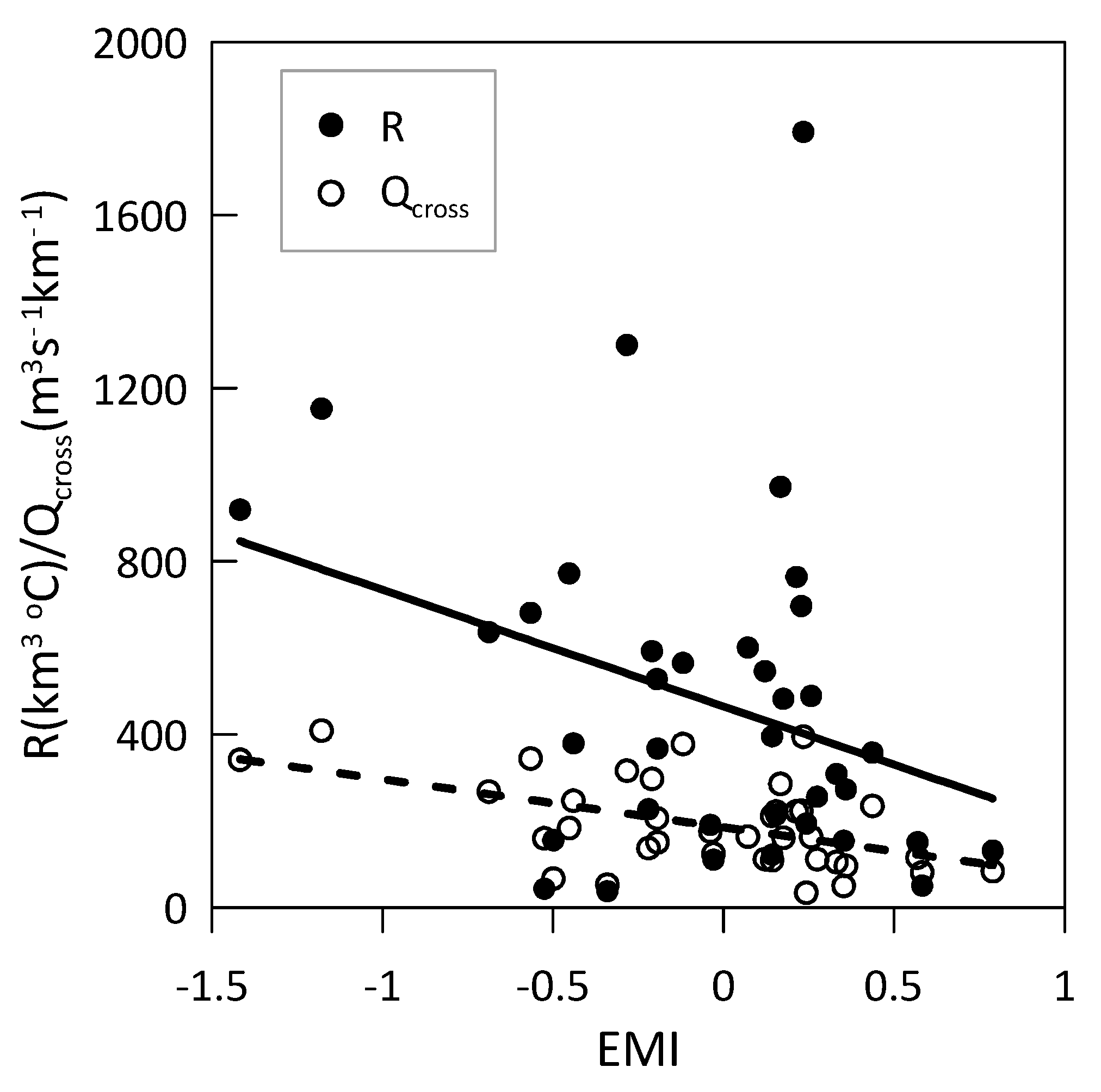
Unlike the delay effect of canonical ENSO events on the changes in summer upwelling in the TWS (Table 2), a negative linear correlation exists in the relationship between R and Qcross with EMI (Figure 7). The correlation coefficient for R/EMI is −0.32 (p = 0.05) and for Qcross/EMI, it is −0.5 (p < 0.01). This result reveals that the El Niño Modoki has a more direct and much stronger impact on the upwelling system of TWS than the canonical El Niño has. During the positive phase of El Niño Modoki, a warm SST anomaly shifted from the east equatorial Pacific to the central equatorial Pacific, which suggests the associated low-level anomalous wind pattern is more distinct and closer to the Asian continent than the canonical ENSO events [56]. Therefore, El Niño Modoki might have a more significant influence on the East Asian summer climate than the canonical El Niño [56].
The East Asian summer monsoon tends to be weaker than normal during strong El Niño Modoki events [57,58] when northeasterly wind anomalies prevail over South China [59]. Strong El Niño Modoki events weaken offshore Ekman transport and are unfavorable for upwelling development. However, the situation is different in the case of La Niña Modoki, when the normal prevailing southwesterly winds are enhanced and the upwelling intensity increases.
To further investigate the impact of ENSO Modoki events on changes in upwelling intensities, we defined strong El Niño Modoki years as the years with average summer EMI > 0.5 and strong La Niña Modoki years as the years with average summer EMI < −0.5. Between 1982 and 2019, the strong El Niño Modoki years included 1994, 2002, and 2004; the strong La Niña Modoki years included 1983, 1997, 1998, 1999, and 2008. Statistics revealed that the average upwelling intensity (R) and Qcross in strong La Niña Modoki years were 5.2 and 2.2 times higher than they were in strong El Niño Modoki years.
Overall, whether considering canonical El Niño or El Niño Modoki, the warm and cold anomaly events associated with these events have played important roles in the interannual or long-term changes of coastal upwelling in the TWS. Some research has pointed out that the upwelling intensity has different response characteristics to different El Niño events [29]. Further quantitative analyses are needed to clarify the influence of ENSO events at their different stages. We do know that the occurrence of El Niño Modoki tends to increase under global warming [60]. Their impacts on the circulation or ecosystem of the TWS should be examined in more detail in future studies.
4.4. Impacts on SST
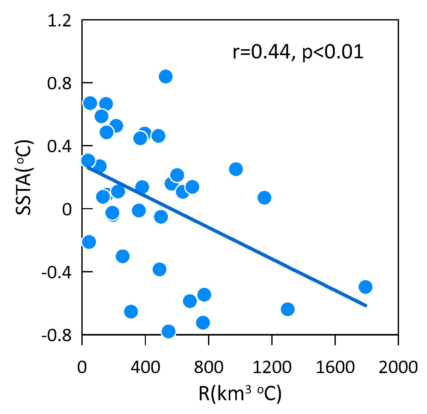
Previous studies have pointed out that upwelling is a key factor buffering ocean warming [61,62]. A general warming was observed at most oceanic and coastal locations in recent decades [63,64]. However, warming has been more intense in offshore than nearshore waters in most of the upwelling locations [61,65,66]. Researchers have demonstrated that enhancing upwelling could hinder the warming due to the continuous pumping of water from intermediate layers. In this study, the negative linear relationship between SSTA and upwelling intensity (Figure 8) in upwelling region of TWS also indicated that increased upwelling could result in a decrease in SST.
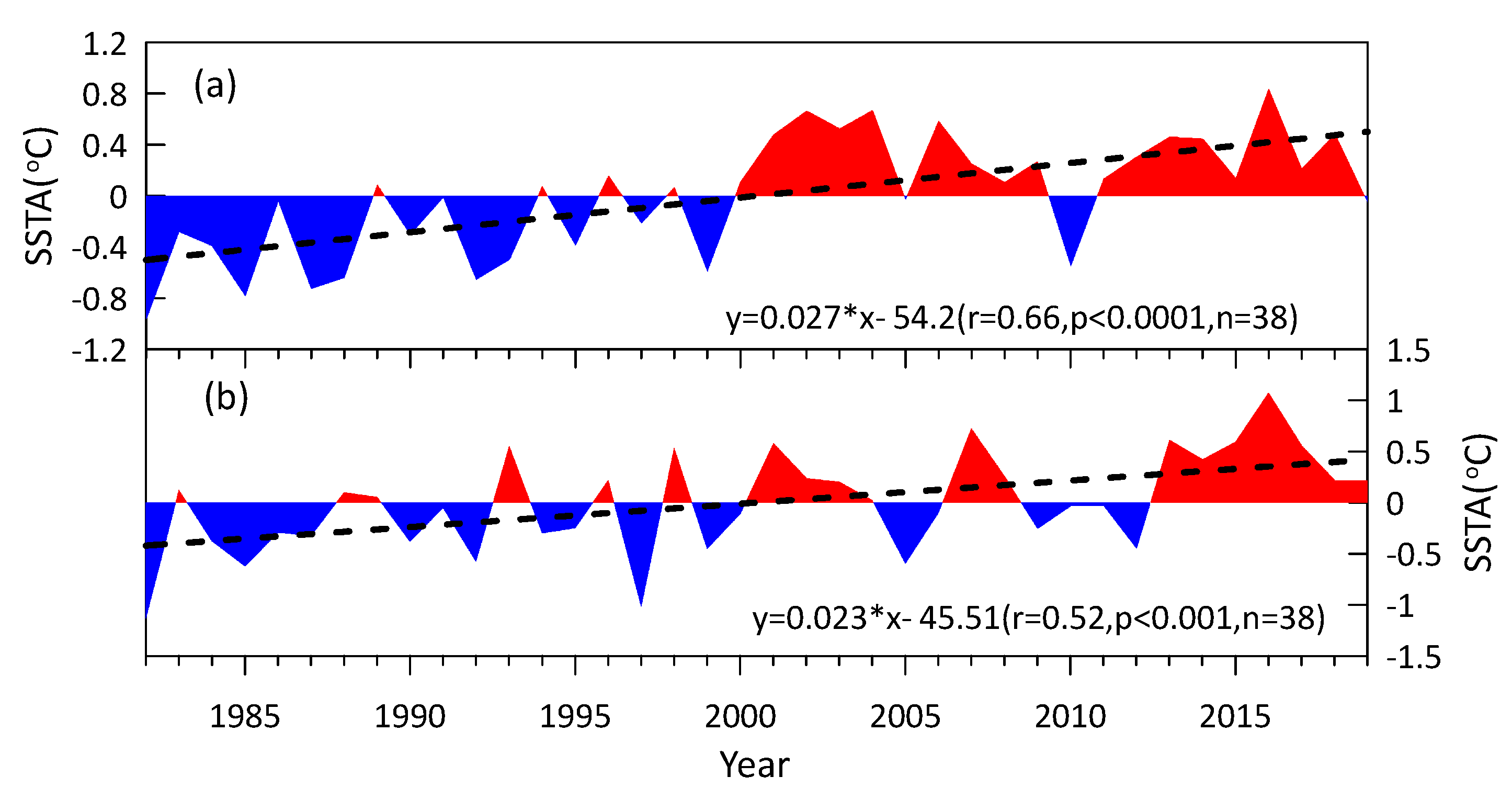
Figure 9 shows that SST increased significantly in the TWS coastal upwelling system (PTU and DSU) from 1982 to 2019. Statistics show that the warming rate of the TWS upwelling region was 0.27 °C/decade, and for the non-upwelling region it was 0.23 °C/decade. The warming rate of the coastal upwelling region was larger than for the non-upwelling region. This finding is in contrast to observations from other upwelling regions such as Benguela, Canary, or California, where a moderate coastal warming or cooling was linked to the intensification of coastal upwelling [67,68].
The underlying mechanism for SST warming was complicated and should be analyzed in future research involving numerical modeling. Nevertheless, the weakened upwelling after 2000 in the TWS (Figure 3 and Table 1) could not slow down the rise rate of SST, possibly due to the reducing vertical transport associated with upwelling. On the other hand, the warming could also produce a deepening of the upper mixed layer and a stronger stratification, which in turn reduce the upwelling intensity.
4.5. Implications for the Upwelling Ecosystem
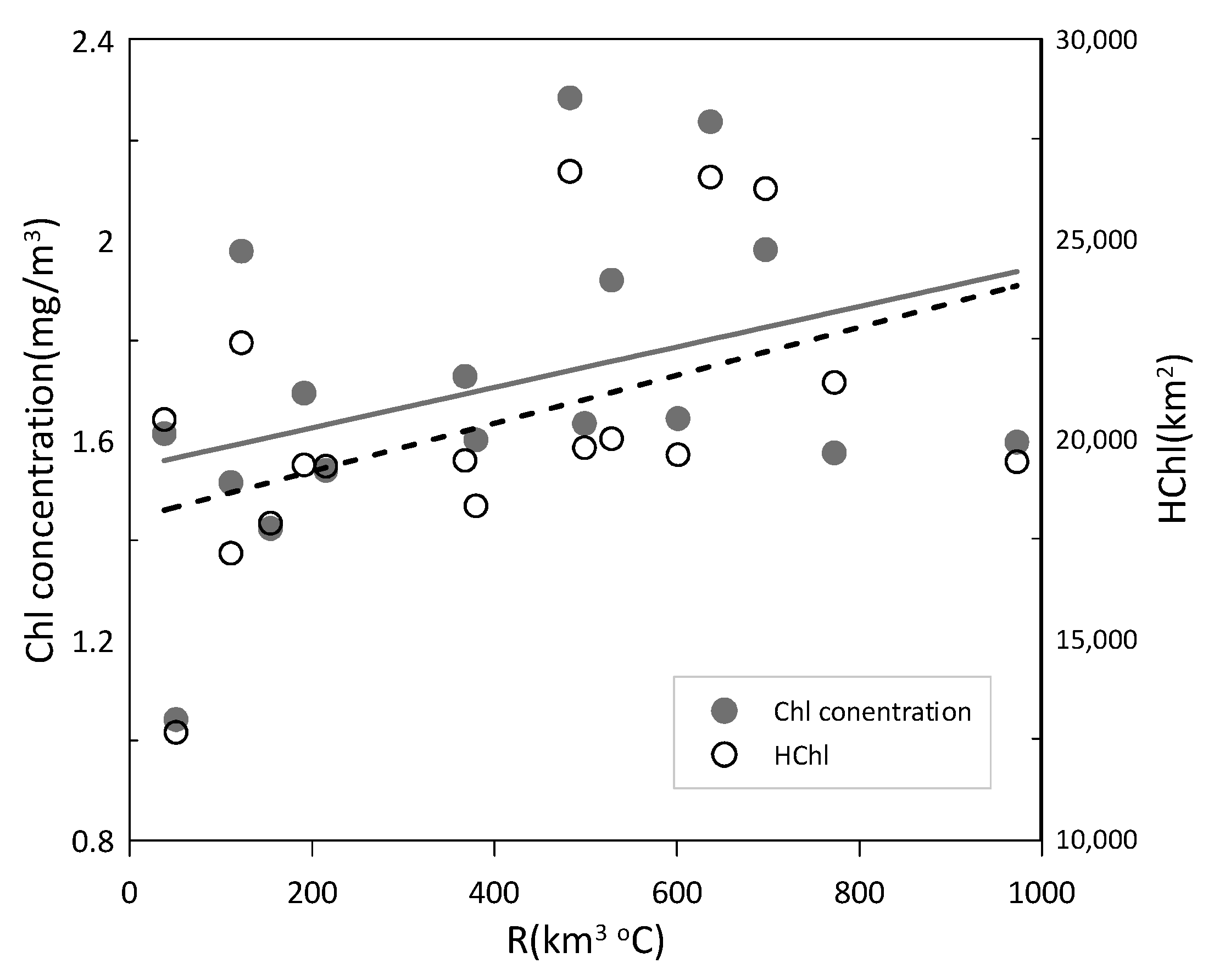
Increased or decreased upwelling has profound implications for biogeochemical and phytoplankton patterns that affect the health of marine ecosystems [48,69,70,71]. We calculated the average Chl and the area of high Chl (Chl ≥ 1 mg/m3) over coastal areas such as PTU and DSU, then investigated their relationship with variations in upwelling intensity, as shown in Figure 10.
The weak positive correlation between upwelling intensity (R) and Chl concentration (Figure 10) indicates that strong upwelling can enhance phytoplankton growth by increasing the nutrient supply from subsurface layers. The correlation coefficients (r) were 0.37 (p = 0.14, n = 17) for Chl concentration and 0.47 (p = 0.057, n = 17) for high Chl area. These results are consistent with other studies from many coastal upwelling regions, which demonstrate that the phytoplankton production can be modified by local supply of nutrients through coastal upwelling [72,73]. The weakened upwelling in the TWS after 2000 (Figure 3 and Table 1) should be not favorable for phytoplankton growth. However, because the MODIS ocean color data are only available after 2002, we cannot compare the variation in Chl concentration before and after 2000. Therefore, maintaining a long time series of consistent ocean-color products is very important for evaluating the impact of climate change on biological fields.
Coastal upwelling regions are “hot spots” with high primary production [74,75]. The alteration of phytoplankton community composition was observed to be associated with different phases of upwelling events [76,77]. In the southern upwelling system of TWS, diatoms dominate in the recently upwelled and mature water. As the upwelled water ages, the community composition shifts rapidly to a coexistence of diatoms and Synechococcus [78]. Based on this pattern, changes in coastal upwelling associated with climate change could impact the base of food chain, then profoundly alter the functioning of marine ecosystems. The Taiwan Strait is one of the important areas in southeast China for fisheries production [13]. Minor changes in local water properties might significantly affect local fishery economics. Therefore, understanding the weakening/enhancing trend of coastal upwelling and the response of biological communities and their ecology will provide key information for predicting how marine ecosystem could react to future climate change.
5. Conclusions
Long-term changes in summer upwelling intensities in the Taiwan Strait were investigated using time series data on sea surface temperature and wind from 1982 to 2019. The results reveal that the summer upwelling of the Taiwan Strait showed a decreased trend with a nonlinear fluctuation over the past four decades. The average upwelling intensity after 2000 was 35% lower than that before 2000. The long-term changes in upwelling intensity are closely correlated with the changes in offshore Ekman transport (Qcross). The offshore Ekman transport also experienced a declined trend after 2000. There was no significant difference in the trend of upwelling intensity in the three subregions of Pingtan upwelling, Dongshan upwelling, and Taiwan Bank upwelling zones. Unlike the delay effect of canonical ENSO events on the changes in summer upwelling, the ENSO Modoki index had a significant negative correlation with upwelling intensity of TWS. Statistics indicated that the average upwelling intensity (R) and Qcross in strong La Niña Modoki years were 5.2 and 2.2 times higher than they were in strong El Niño Modoki years. Strong El Niño Modoki events were not favorable for the development of upwelling. Moreover, the decreased upwelling did not slow down the warming rate of sea surface temperature and could cause the decline of chlorophyll a in the coastal upwelling system of TWS.
SST and winds are important indicators for understanding variations in upwelling and the potential ecological response. Although changes in tide, stratification, currents, or other processes can contribute to the changes of upwelling, some of their effects in climate change scenarios are difficult to access or predict [66]. Thus, although more research is necessary, studies such as this one are a starting point for evaluating future trends in coastal upwelling and their potential ecological effects in the Taiwan Strait.
Funding
This research was funded by the National Key Research and Development Plan of China (Grant No. 2016YFE0202100) and the Key Program of NSF-China (Grant No. U1805241).
Data Availability Statement
Publicly available data sets were analyzed in this study. AVHRR sea surface temperature data can be found here: http://pathfinder.nodc.noaa.gov (accessed on 5 March 2021). ERA5 wind data can be found here: http://apdrc.soest.hawaii.edu/ (accessed on 5 March 2021). MODIS chlorophyll a data can be found here: http://oceancolor.gsfc.nasa.gov (accessed on 5 March 2021).
Acknowledgments
Anonymous reviewers contributed substantially to the improvement of this paper.
Conflicts of Interest
The author declares no conflict of interest.
References
- Chavez, F.; Pennington, J.; Castro, C.; Ryan, J.; Michisaki, R.; Schlining, B.; Walz, P.; Buck, K.; McFadyen, A.; Collins, C. Biological and chemical consequences of the 1997–1998 el niño in central california waters. Prog. Oceanogr. 2002, 54, 205–232. [Google Scholar] [CrossRef]
- Bakun, A.; Field, D.B.; Redondo-Rodriguez, A.; Weeks, S.J. Greenhouse gas, upwelling-favorable winds, and the future of coastal ocean upwelling ecosystems. J. Glob. Chang. Biol. 2010, 16, 1213–1228. [Google Scholar] [CrossRef]
- Bakun, A. Global climate change and intensification of coastal ocean upwelling. Science 1990, 247, 198–201. [Google Scholar] [CrossRef] [Green Version]
- McGregor, H.; Dima, M.; Fischer, H.W.; Mulitza, S. Rapid 20th-century increase in coastal upwelling off northwest africa. Science 2007, 315, 637–639. [Google Scholar] [CrossRef]
- Sydeman, W.; García-Reyes, M.; Schoeman, D.; Rykaczewski, R.; Thompson, S.; Black, B.A.; Bograd, S. Climate change and wind intensification in coastal upwelling ecosystems. Science 2014, 345, 77–80. [Google Scholar] [CrossRef]
- Sousa, M.C.; Ribeiro, A.; Des, M.; Gomez-Gesteira, M.; de Castro, M.; Dias, J.M. Nw iberian peninsula coastal upwelling future weakening: Competition between wind intensification and surface heating. Sci. Total. Environ. 2020, 703, 134808. [Google Scholar] [CrossRef] [PubMed]
- Wang, D.; Gouhier, T.C.; Menge, B.A.; Ganguly, A.R. Intensification and spatial homogenization of coastal upwelling under climate change. Nature 2015, 518, 390–394. [Google Scholar] [CrossRef]
- Rykaczewski, R.R.; Dunne, J.P.; Sydeman, W.J.; García-Reyes, M.; Black, B.A.; Bograd, S.J. Poleward displacement of coastal upwelling-favorable winds in the ocean’s eastern boundary currents through the 21st century. Geophys. Res. Lett. 2015, 42, 6424–6431. [Google Scholar] [CrossRef]
- Varela, R.; Álvarez, I.; Santos, F.; DeCastro, M.; Gómez-Gesteira, M. Has upwelling strengthened along worldwide coasts over 1982–2010? Sci. Rep. 2015, 5, 1–15. [Google Scholar] [CrossRef]
- Relvas, P.; Luís, J.; Santos, A.M.P. Importance of the mesoscale in the decadal changes observed in the northern canary upwelling system. Geophys. Res. Lett. 2009, 36. [Google Scholar] [CrossRef]
- Liu, Y.; Peng, Z.; Shen, C.C.; Zhou, R.; Song, S.; Shi, Z.; Chen, T.; Wei, G.; DeLong, K.L. Recent 121-year variability of western boundary upwelling in the northern south china sea. Geophys. Res. Lett. 2013, 40, 3180–3183. [Google Scholar] [CrossRef]
- Jan, S.; Wang, J.; Chern, C.-S.; Chao, S.-Y. Seasonal variation of the circulation in the taiwan strait. J. Mar. Syst. 2002, 35, 249–268. [Google Scholar] [CrossRef]
- Hong, H.S.; Chai, F.; Zhang, C.Y.; Huang, B.Q.; Jiang, Y.W.; Hu, J.Y. An overview of physical and biogeochemical processes and ecosystem dynamics in the taiwan strait. Cont. Shelf Res. 2011, 31, S3–S12. [Google Scholar] [CrossRef]
- Hu, J.Y.; Kawamura, H.; Hong, H.S.; Pan, W.R. A review of research on the upwelling in the taiwan strait. Bull. Mar. Sci. 2003, 73, 605–628. [Google Scholar]
- Tang, D.; Kester, D.R.; Ni, I.H.; Kawamura, H.; Hong, H. Upwelling in the taiwan strait during the summer monsoon detected by satellite and shipboard measurements. Remote Sens. Environ. 2002, 83, 457–471. [Google Scholar] [CrossRef]
- Jiang, Y.; Chai, F.; Wan, Z.; Zhang, X.; Hong, H. Characteristics and mechanisms of the upwelling in the southern taiwan strait: A three-dimensional numerical model study. J. Oceanogr. 2011, 67, 699–708. [Google Scholar] [CrossRef]
- Hu, J.-y.; Kawamura, H.; Hong, H.-s.; Suetsugu, M.; Lin, M.-s. Hydrographic and satellite observations of summertime upwelling in the taiwan strait: A preliminary description. Terr. Atmos. Ocean. Sci. 2001, 12, 415–430. [Google Scholar] [CrossRef] [Green Version]
- Chen, Z.; Yan, X.H.; Jiang, Y. Coastal cape and canyon effects on wind-driven upwelling in northern taiwan strait. J. Geophys. Res. Ocean. 2014, 119, 4605–4625. [Google Scholar] [CrossRef]
- Cai, W.; Lennon, G. Upwelling in the taiwan strait in response to wind stress, ocean circulation and topography. Estuar. Coast. Shelf Sci. 1988, 26, 15–31. [Google Scholar]
- Huang, B.; Xiang, W.; Zeng, X.; Chiang, K.-P.; Tian, H.; Hu, J.; Lan, W.; Hong, H. Phytoplankton growth and microzooplankton grazing in a subtropical coastal upwelling system in the taiwan strait. Cont. Shelf Res. 2011, 31, S48–S56. [Google Scholar] [CrossRef]
- Xiao, H. Studies of coastal upwelling in western taiwan strait. J. Oceanogr. Taiwan Strait 1988, 7, 135–142. [Google Scholar]
- Wang, Y.; Kang, J.-H.; Ye, Y.-Y.; Lin, G.-M.; Yang, Q.-L.; Lin, M. Phytoplankton community and environmental correlates in a coastal upwelling zone along western taiwan strait. J. Mar. Syst. 2016, 154, 252–263. [Google Scholar] [CrossRef]
- Zhang, C.Y.; Hong, H.S.; Ru, C.M.; Shang, S.L. Evolution of a coastal upwelling event during summer 2004 in the southern taiwan strait. Acta Oceanol. Sin. 2011, 30, 1–6. [Google Scholar] [CrossRef]
- Shang, S.L.; Zhang, C.Y.; Hong, H.S.; Shang, S.P.; Chai, F. Short-term variability of chlorophyll associated with upwelling events in the taiwan strait during the southwest monsoon of 1998. Deep Sea Res. Part II Top. Stud. Oceanogr. 2004, 51, 1113–1127. [Google Scholar] [CrossRef]
- Tang, D.L.; Kawamura, H.; Guan, L. Long-time observation of annual variation of taiwan strait upwelling in summer season. Adv. Space Res. 2004, 33, 307–312. [Google Scholar] [CrossRef]
- Hong, H.; Zhang, C.; Shang, S.; Huang, B.; Li, Y.; Li, X.; Zhang, S. Interannual variability of summer coastal upwelling in the taiwan strait. Cont. Shelf Res. 2009, 29, 479–484. [Google Scholar] [CrossRef]
- Belkin, I.M.; Lee, M.A. Long-term variability of sea surface temperature in taiwan strait. Clim. Chang. 2014, 124, 821–834. [Google Scholar] [CrossRef] [Green Version]
- Zhang, C.; Huang, Y.; Ding, W. Enhancement of zhe-min coastal water in the taiwan strait in winter. J. Oceanogr. 2020, 76, 197–209. [Google Scholar] [CrossRef]
- Jacox, M.G.; Fiechter, J.; Moore, A.M.; Edwards, C.A. Enso and the c alifornia c urrent coastal upwelling response. J. Geophys. Res. Ocean. 2015, 120, 1691–1702. [Google Scholar] [CrossRef]
- Roy, C.; Reason, C. Enso related modulation of coastal upwelling in the eastern atlantic. Prog. Oceanogr. 2001, 49, 245–255. [Google Scholar] [CrossRef]
- Wolter, K.; Timlin, M.S. Measuring the strength of enso events—how does 1997/98 rank? Weather 1998, 53, 315–324. [Google Scholar] [CrossRef]
- Ashok, K.; Behera, S.K.; Rao, S.A.; Weng, H.; Yamagata, T. El niño modoki and its possible teleconnection. J. Geophys. Res. Ocean. 2007, 112, C11. [Google Scholar] [CrossRef]
- Shang, S.; Zhang, C.; Hong, H.; Liu, Q.; Wong, G.T.F.; Hu, C.; Huang, B. Hydrographic and biological changes in the taiwan strait during the 1997–1998 el nino winter. Geophys. Res. Lett. 2005, 32, 4. [Google Scholar] [CrossRef] [Green Version]
- Kuo, N.J.; Ho, C.R. Enso effect on the sea surface wind and sea surface temperature in the taiwan strait. Geophys. Res. Lett 2004, 31, L13309. [Google Scholar] [CrossRef]
- Saha, K.; Zhao, X.; Zhang, H.; Casey, K.; Zhang, D.; Baker-Yeboah, S.; Kilpatrick, K.; Evans, R.; Ryan, T.; Relph, J. Avhrr Pathfinder Version 5.3 Level 3 Collated (l3c) Global 4km Sea Surface Temperature for 1981-Present; NOAA National Centers for Environmental Information: Washington, DC, USA, 2018. [Google Scholar]
- Qiu, C.; Wang, D.; Kawamura, H.; Guan, L.; Qin, H. Validation of avhrr and tmi-derived sea surface temperature in the northern south china sea. Cont. Shelf Res. 2009, 29, 2358–2366. [Google Scholar] [CrossRef]
- O’Carroll, A.G.; Armstrong, E.M.; Beggs, H.M.; Bouali, M.; Casey, K.S.; Corlett, G.K.; Dash, P.; Donlon, C.J.; Gentemann, C.L.; Høyer, J.L. Observational needs of sea surface temperature. Front. Mar. Sci. 2019, 6, 420. [Google Scholar] [CrossRef]
- Kuo, N.-J.; Zheng, Q.; Ho, C.-R. Satellite observation of upwelling along the western coast of the south china sea. Remote Sens. Environ. 2000, 74, 463–470. [Google Scholar] [CrossRef]
- Pond, S.; Pickard, G.L. Introductory Dynamical Oceanography, 2nd ed.; Butterworth-Heinemann: Oxford, UK, 1983. [Google Scholar]
- Trenberth, K.E.; Large, W.G.; Olson, J.G. The mean annual cycle in global ocean wind stress. J. Phys. Oceanogr. 1990, 20, 1742–1760. [Google Scholar] [CrossRef] [Green Version]
- Cropper, T.E.; Hanna, E.; Bigg, G.R. Spatial and temporal seasonal trends in coastal upwelling off northwest africa, 1981–2012. Deep Sea Res. I 2014, 86, 94–111. [Google Scholar] [CrossRef] [Green Version]
- Lee, H.W.; Bhang, K.J.; Park, S.S. Effective visualization for the spatiotemporal trend analysis of the water quality in the nakdong river of korea. Ecol. Inform. 2010, 5, 281–292. [Google Scholar] [CrossRef]
- Cleveland, W.S. Robust locally weighted regression and smoothing scatter plots. J. Am. Stat. Assoc. 1979, 74, 829–836. [Google Scholar] [CrossRef]
- Richards, R.P.; Baker, D.B. Trends in water quality in leaseq rivers and streams (northwestern ohio), 1975–1995. J. Environ. Qual. 2002, 31, 90–96. [Google Scholar] [CrossRef]
- Xie, L.; Zong, X.; Yi, X.; Li, M. The interannual variation and long-term trend of qiongdong upwelling. Oceanol. Limnol. Sin. 2016, 47, 43–51. [Google Scholar]
- Yang, S.; Mao, X.; Jiang, W. Interannual variation of coastal upwelling in summer in zhejiang, china. Period. Ocean Univ. China 2020, 50, 1–8. [Google Scholar]
- Pérez, F.F.; Padín, X.A.; Pazos, Y.; Gilcoto, M.; Cabanas, M.; Pardo, P.C.; Doval, M.D.; FARINA-BUSTO, L. Plankton response to weakening of the iberian coastal upwelling. Glob. Chang. Biol. 2010, 16, 1258–1267. [Google Scholar] [CrossRef] [Green Version]
- García-Reyes, M.; Sydeman, W.J.; Schoeman, D.S.; Rykaczewski, R.R.; Black, B.A.; Smit, A.J.; Bograd, S.J. Under pressure: Climate change, upwelling, and eastern boundary upwelling ecosystems. Front. Mar. Sci. 2015, 2, 109. [Google Scholar] [CrossRef] [Green Version]
- Xu, M.; Chang, C.P.; Fu, C.; Qi, Y.; Robock, A.; Robinson, D.; Zhang, H.m. Steady decline of east asian monsoon winds, 1969–2000: Evidence from direct ground measurements of wind speed. J. Geophys. Res. Atmos. 2006, 111, D24111. [Google Scholar] [CrossRef] [Green Version]
- Zuo, Z.; Yang, S.; Kumar, A.; Zhang, R.; Xue, Y.; Jha, B. Role of thermal condition over asia in the weakening asian summer monsoon under global warming background. J. Clim. 2012, 25, 3431–3436. [Google Scholar] [CrossRef]
- Wang, D.; Shu, Y.; Xue, H.; Hu, J.; Chen, J.; Zhuang, W.; Zu, T.; Xu, J. Relative contributions of local wind and topography to the coastal upwelling intensity in the northern south china sea. J. Geophys. Res. Ocean. 2014, 119, 2550–2567. [Google Scholar] [CrossRef]
- Zhang, W.Z.; Shi, F.; Hong, H.S.; Shang, S.P.; Kirby, J.T. Tide-surge interaction intensified by the taiwan strait. J. Geophys. Res. Ocean. 2010, 115, C6. [Google Scholar] [CrossRef] [Green Version]
- Wang, B.; Wu, R.; Fu, X. Pacific–east asian teleconnection: How does enso affect east asian climate? J. Clim. 2000, 13, 1517–1536. [Google Scholar] [CrossRef]
- Pan, J.; Yan, X.-H.; Zheng, Q.; Liu, W.T.; Klemas, V.V. Interpretation of scatterometer ocean surface wind vector eofs over the northwestern pacific. Remote Sens. Environ. 2003, 84, 53–68. [Google Scholar] [CrossRef]
- Li, N.; Shang, S.P.; Shang, S.L.; Zhang, C.Y. On the consistency in variations of the south china sea warm pool as revealed by three sea surface temperature datasets. Remote Sens. Environ. 2007, 109, 118–125. [Google Scholar] [CrossRef]
- Chen, Z.; Wen, Z.; Wu, R.; Zhao, P.; Cao, J. Influence of two types of el niños on the east asian climate during boreal summer: A numerical study. Clim. Dyn. 2014, 43, 469–481. [Google Scholar] [CrossRef]
- Yuan, Y.; Yang, S. Impacts of different types of el niño on the east asian climate: Focus on enso cycles. J. Clim. 2012, 25, 7702–7722. [Google Scholar] [CrossRef]
- Weng, H.; Ashok, K.; Behera, S.K.; Rao, S.A.; Yamagata, T. Impacts of recent el niño modoki on dry/wet conditions in the pacific rim during boreal summer. Clim. Dyn. 2007, 29, 113–129. [Google Scholar] [CrossRef]
- Feng, J.; Li, J. Influence of el niño modoki on spring rainfall over south china. J. Geophys. Res. Atmos. 2011, 116. [Google Scholar] [CrossRef]
- Yeh, S.-W.; Kug, J.-S.; Dewitte, B.; Kwon, M.-H.; Kirtman, B.P.; Jin, F.-F.J.N. El niño in a changing climate. Nature 2009, 461, 511–514. [Google Scholar] [CrossRef]
- Varela, R.; Lima, F.P.; Seabra, R.; Meneghesso, C.; Gómez-Gesteira, M. Coastal warming and wind-driven upwelling: A global analysis. Sci. Total. Environ. 2018, 639, 1501–1511. [Google Scholar] [CrossRef] [PubMed]
- Santos, F.; Gómez-Gesteira, M.; Varela, R.; Ruiz-Ochoa, M.; Días, J.M. Influence of upwelling on sst trends in la guajira system. J. Geophys. Res. Ocean. 2016, 121, 2469–2480. [Google Scholar] [CrossRef] [Green Version]
- Casey, K.S.; Cornillon, P. Global and regional sea-surface temperature trends. J. Clim. 2001, 14, 3801–3818. [Google Scholar] [CrossRef] [Green Version]
- Liao, E.H.; Lu, W.F.; Yan, X.H.; Jiang, Y.W.; Kidwell, A. The coastal ocean response to the global warming acceleration and hiatus. Sci. Rep. 2015, 5, 10. [Google Scholar] [CrossRef] [Green Version]
- Santos, F.; de Castro, M.; Gómez-Gesteira, M.; Álvarez, I. Differences in coastal and oceanic sst warming rates along the canary upwelling ecosystem from 1982 to 2010. Cont. Shelf Res. 2012, 47, 1–6. [Google Scholar] [CrossRef]
- Sousa, M.C.; Alvarez, I.; de Castro, M.; Gomez-Gesteira, M.; Dias, J.M. Seasonality of coastal upwelling trends under future warming scenarios along the southern limit of the canary upwelling system. Prog. Oceanogr. 2017, 153, 16–23. [Google Scholar] [CrossRef]
- Arellano, B.; Rivas, D. Coastal upwelling will intensify along the baja california coast under climate change by mid-21st century: Insights from a gcm-nested physical-npzd coupled numerical ocean model. J. Mar. Syst. 2019, 199, 103207. [Google Scholar] [CrossRef]
- Seabra, R.; Varela, R.; Santos, A.; Gómez-Gesteira, M.; Meneghesso, C.; Wethey, D.; Lima, F. Reduced nearshore warming associated with eastern boundary upwelling systems. Front. Mar. Sci. 2019, 6, 104. [Google Scholar] [CrossRef] [Green Version]
- Xiu, P.; Chai, F.; Curchitser, E.N.; Castruccio, F.S. Future changes in coastal upwelling ecosystems with global warming: The case of the california current system. Sci. Rep. 2018, 8, 2866. [Google Scholar] [CrossRef]
- Di Lorenzo, E. The future of coastal ocean upwelling. Nature 2015, 518, 310–311. [Google Scholar] [CrossRef]
- Miranda, P.; Alves, J.; Serra, N. Climate change and upwelling: Response of iberian upwelling to atmospheric forcing in a regional climate scenario. Clim. Dyn. 2013, 40, 2813–2824. [Google Scholar] [CrossRef]
- Chavez, F.P.; Messié, M. A comparison of eastern boundary upwelling ecosystems. Prog. Oceanogr. 2009, 83, 80–96. [Google Scholar] [CrossRef]
- Lass, H.-U.; Mohrholz, V.; Nausch, G.; Siegel, H. On phosphate pumping into the surface layer of the eastern gotland basin by upwelling. J. Mar. Syst. 2010, 80, 71–89. [Google Scholar] [CrossRef]
- Dugdale, R.; Wilkerson, F. New production in the upwelling center at point conception, california: Temporal and spatial patterns. Deep Sea Res. Part A Oceanogr. Res. Pap. 1989, 36, 985–1007. [Google Scholar] [CrossRef]
- Largier, J.L. Upwelling bays: How coastal upwelling controls circulation, habitat, and productivity in bays. Annu. Rev. Mar. Sci. 2020, 12, 415–447. [Google Scholar] [CrossRef] [PubMed]
- Mitchell-Innes, B.; Walker, D. Short-term variability during an anchor station study in the southern benguela upwelling system: Phytoplankton production and biomass in relation to specie changes. Prog. Oceanogr. 1991, 28, 65–89. [Google Scholar] [CrossRef]
- Bettencourt, J.H.; Rossi, V.; Renault, L.; Haynes, P.; Morel, Y.; Garçon, V. Effects of upwelling duration and phytoplankton growth regime on dissolved-oxygen levels in an idealized iberian peninsula upwelling system. Nonlinear Process. Geophys. 2020, 27, 277–294. [Google Scholar] [CrossRef]
- Zhong, Y.; Hu, J.; Laws, E.A.; Liu, X.; Chen, J.; Huang, B. Plankton community responses to pulsed upwelling events in the southern taiwan strait. ICES J. Mar. Sci. 2019, 76, 2374–2388. [Google Scholar] [CrossRef]
Figure 1.
Map of the study area, overlaid with the bathymetry contours in meters. TWS: Taiwan Strait; ECS: East China Sea; SCS: South China Sea; Is.: Island.
Figure 1.
Map of the study area, overlaid with the bathymetry contours in meters. TWS: Taiwan Strait; ECS: East China Sea; SCS: South China Sea; Is.: Island.

Figure 2.
The spatial distribution of the difference in SST between the TWS and non−upwelling zone (a) and the SST gradient (b) of multi−year average summer sea surface temperature for 1982–2019 in the TWS. The calculation domain for the Pingtan upwelling (PTU), Dongshan upwelling (DSU), Taiwan Bank upwelling (TBU), and non−upwelling zone (N) are illustrated as red dashed lines on (a). The overlaid white contours represent a SST difference of −2 °C.

Figure 3.
Temporal variation in upwelling intensity (R) from 1982 to 2019 for the Pingtan upwelling (PTU, a), Dongshan upwelling (DSU, b), and Taiwan Bank upwelling (TBU, c). The blue dotted lines and grey dashed lines represent the LOWESS fit lines and linear fit lines, respectively.
Figure 3.
Temporal variation in upwelling intensity (R) from 1982 to 2019 for the Pingtan upwelling (PTU, a), Dongshan upwelling (DSU, b), and Taiwan Bank upwelling (TBU, c). The blue dotted lines and grey dashed lines represent the LOWESS fit lines and linear fit lines, respectively.

Figure 4.
Variation in upwelling intensity (R) over four different periods.

Figure 5.
Temporal variation of cross−shore Ekman transport (Qcross) from 1982 to 2019 for PTU (a), DSU (b), and TBU (c). The blue dotted lines and grey dashed liens represent the LOWESS fit lines and linear fit lines, respectively.
Figure 5.
Temporal variation of cross−shore Ekman transport (Qcross) from 1982 to 2019 for PTU (a), DSU (b), and TBU (c). The blue dotted lines and grey dashed liens represent the LOWESS fit lines and linear fit lines, respectively.

Figure 6.
Relationship between the cross−shore Ekman transport (Qcross) and upwelling intensity (R) in PTU (a), DSU (b), and TBU (c).
Figure 6.
Relationship between the cross−shore Ekman transport (Qcross) and upwelling intensity (R) in PTU (a), DSU (b), and TBU (c).

Figure 7.
Relationship between upwelling intensity (R), Qcross, and EMI for the coastal upwelling system of the Taiwan Strait.
Figure 7.
Relationship between upwelling intensity (R), Qcross, and EMI for the coastal upwelling system of the Taiwan Strait.

Figure 8.
Relationship between upwelling intensity (R) and SSTA for the coastal upwelling system of the Taiwan Strait.
Figure 8.
Relationship between upwelling intensity (R) and SSTA for the coastal upwelling system of the Taiwan Strait.

Figure 9.
Variation in SSTA for coastal upwelling region (a) and non−upwelling region (b) during 1982–2019.
Figure 9.
Variation in SSTA for coastal upwelling region (a) and non−upwelling region (b) during 1982–2019.

Figure 10.
Relationship between upwelling intensity (R) and chlorophyll a (Chl) concentration and the area of high Chl (HChl) for the coastal upwelling system of the Taiwan Strait.
Figure 10.
Relationship between upwelling intensity (R) and chlorophyll a (Chl) concentration and the area of high Chl (HChl) for the coastal upwelling system of the Taiwan Strait.


Table 1.
Statistical results in the change of R and Qcross before 2000 and after 2000.
| R | Qcross | |||||
|---|---|---|---|---|---|---|
| PTU | DSU | TBU | PTU | DSU | TBU | |
| 1982–1999 | 610.0 ± 480.0 | 559.5 ± 461.3 | 564.8 ± 427.9 | 256 ± 160.3 | 174.4 ± 94.9 | 220.8 ± 87.0 |
| 2000–2019 | 326.1 ± 250.2 | 433.2 ± 329.3 | 356.6 ± 276.6 | 185.9 ± 84.3 | 149.0 ± 55.3 | 187.1 ± 52.8 |
| Change rate | −46% | −22% | −37% | −27% | −14% | −15% |
Table 2.
Lag correlation coefficients between Multivariate ENSO (El Niño/Southern Oscillation) Index (MEI) and R and Qcross, respectively.
Table 2.
Lag correlation coefficients between Multivariate ENSO (El Niño/Southern Oscillation) Index (MEI) and R and Qcross, respectively.
| Lag(month) | R(p) | Qcross(p) |
|---|---|---|
| 0 | −0.205(0.216) | −0.218(0.187) |
| −3 | 0.430(<0.01) | 0.331(<0.05) |
| −6 | 0.470(<0.01) | 0.330(<0.05) |
| −9 | 0.451(<0.01) | 0.312(0.056) |
| −12 | 0.526(<0.01) | 0.443(<0.05) |
Publisher’s Note: MDPI stays neutral with regard to jurisdictional claims in published maps and institutional affiliations. |
© 2021 by the author. Licensee MDPI, Basel, Switzerland. This article is an open access article distributed under the terms and conditions of the Creative Commons Attribution (CC BY) license (https://creativecommons.org/licenses/by/4.0/).
Share and Cite
MDPI and ACS Style
Zhang, C. Responses of Summer Upwelling to Recent Climate Changes in the Taiwan Strait. Remote Sens. 2021, 13, 1386. https://0-doi-org.brum.beds.ac.uk/10.3390/rs13071386
AMA Style
Zhang C. Responses of Summer Upwelling to Recent Climate Changes in the Taiwan Strait. Remote Sensing. 2021; 13(7):1386. https://0-doi-org.brum.beds.ac.uk/10.3390/rs13071386
Chicago/Turabian StyleZhang, Caiyun. 2021. "Responses of Summer Upwelling to Recent Climate Changes in the Taiwan Strait" Remote Sensing 13, no. 7: 1386. https://0-doi-org.brum.beds.ac.uk/10.3390/rs13071386
Note that from the first issue of 2016, this journal uses article numbers instead of page numbers. See further details here.