Article

A New Method for Determining an Optimal Diurnal Threshold of GNSS Precipitable Water Vapor for Precipitation Forecasting

1
School of Environment Science and Spatial Informatics, China University of Mining and Technology, No.1 Daxue Road, Xuzhou 221116, China
2
Aerospace Information Research Institute, Chinese Academy of Sciences, No.9 Dengzhuang South Road, Haidian District, Beijing 100094, China
3
Satellite Positioning for Atmosphere, Climate and Environment (SPACE) Research Center, RMIT University, 124 La Trobe St, Melbourne, VIC 3000, Australia
4
Bei-stars Geospatial Information Innovation Institute, No. 1 Xinbei Road, Pukou District, Nanjing 210000, China
5
Research Center of Beidou Navigation and Remote Sensing, Suzhou University of Science and Technology, Suzhou 215009, China
*
Author to whom correspondence should be addressed.
Submission received: 1 March 2021 / Revised: 28 March 2021 / Accepted: 31 March 2021 / Published: 4 April 2021
(This article belongs to the Special Issue Climate Modelling and Monitoring Using GNSS)

Abstract

:
Nowadays, precipitable water vapor (PWV) retrieved from ground-based Global Navigation Satellite Systems (GNSS) tracking stations has heralded a new era of GNSS meteorological applications, especially for severe weather prediction. Among the existing models that use PWV timeseries to predict heavy precipitation, the “threshold-based” models, which are based on a set of predefined thresholds for the predictors used in the model for predictions, are effective in heavy precipitation nowcasting. In previous studies, monthly thresholds have been widely accepted due to the monthly patterns of different predictors being fully considered. However, the primary weakness of this type of thresholds lies in their poor prediction results in the transitional periods between two consecutive months. Therefore, in this study, a new method for the determination of an optimal set of diurnal thresholds by adopting a 31-day sliding window was first proposed. Both the monthly and diurnal variation characteristics of the predictors were taken into consideration in the new method. Then, on the strength of the new method, an improved PWV-based model for heavy precipitation prediction was developed using the optimal set of diurnal thresholds determined based on the hourly PWV and precipitation records for the summer over the period 2010–2017 at the co-located HKSC–KP (King’s Park) stations in Hong Kong. The new model was evaluated by comparing its prediction results against the hourly precipitation records for the summer in 2018 and 2019. It is shown that 96.9% of heavy precipitation events were correctly predicted with a lead time of 4.86 h, and the false alarms resulting from the new model were reduced to 25.3%. These results suggest that the inclusion of the diurnal thresholds can significantly improve the prediction performance of the model.

Graphical Abstract

1. Introduction

Atmospheric water vapor, as one of the main greenhouse gases, plays an important role in meteorological applications and is often expressed in the form of precipitable water vapor (PWV), which has been estimated using the Global Navigation Satellite Systems (GNSS) technique since the early 1990s [1]. Generally, observations using the GNSS radio signals, i.e., ground- and space-based GNSS observations, are regarded as complements to those in-situ and remotely sensed observations for the understanding and prediction of extreme weather events [2,3,4]. Nowadays, with the rapid development of the GNSS and the widespread establishment of various scale ground-based tracking networks, the application of the GNSS-derived PWV (named GNSS-PWV hereinafter) to climate research and weather predictions has been well advanced [5,6,7,8], especially for severe weather events [9,10]. This is due to the high accuracy, high spatiotemporal resolution, and all-weather availability of the GNSS-PWV [11,12,13,14]. Several methods using GNSS-PWV for precipitation prediction have been proposed in recent years. Yao et al. [15] proposed a new model containing the three predictors of PWV value, PWV variation, and rate of PWV variation. Based on data collected at GNSS tracking stations in Zhejiang Province, the model led to an 82% correct detection rate but high false alarm rates (FAR): 60–70%. Zhao et al. [16] developed an improved model based on GNSS-PWV timeseries with a 5-minute resolution, and the model resulted in a better than 90% correct detection rate. In our previous study [17], a new model including five predictors derived from GNSS-PWV timeseries was developed, and the model’s probability of detection (POD) and FAR were 95.5% and 28.9%, respectively. Apart from these threshold-based models, for which a set of predefined thresholds for the predictors adopted in the model were used to make predictions, the neural network (NN) technique has also been applied to precipitation prediction by incorporating PWV with other atmospheric parameters as input variables of the model [18,19]. Benevides et al. [20] presented a nonlinear autoregressive exogenous neural network model developed based on the integration of GNSS and meteorological data for the short-term prediction of intense precipitation events. Although the model resulted in a reduced FAR, from 36% to 21%, its 72% POD score was undesirable. Manandhar et al. [21] proposed a data-driven method using seven variables including GNSS-PWV to predict precipitation events, which showed an 80.4% POD and a 20.3% FAR. Furthermore, based on the maturing data assimilation technique, GNSS-PWV was also assimilated into the operational numerical weather prediction (NWP) models, which could effectively improve the monitoring and prediction of precipitation events [22,23,24,25].
All the aforementioned types of models using PWV timeseries for precipitation prediction, albeit the NWP models have a solid theoretical basis, are still difficult to be applied to the nowcasting of heavy precipitation events, while those NN-based models cannot provide insight into their interior structures and physical processes of the modelling, due to their “black box” feature. Therefore, this study is mainly focused on the threshold-based models, which are easy to operate and can be used as effective complements to operational models. Generally speaking, the selection of appropriate predictors and the determination of an optimal set of thresholds for these predictors are the keys for the development of a threshold-based model. The selection of predictors can be different depending on various factors, such as the type of target events, availability of sample data, and climate patterns. Hence, it is difficult to establish a common standard. However, the thresholds for those predefined predictors can be determined based on some certain rules, and several methods have been proposed recently [26,27,28]. Zhao et al. [29] used the percentile method, which shows the location and distribution of the sample data through the median and quartile [30], to determine an optimal set of thresholds. In the studies [15,31], empirical thresholds for predictors were simply selected from values given within a certain range without justification. In contrast, in our recent study [17], an optimal set of thresholds were determined according to the critical success index (CSI), and each predictor in each summer month had a unique threshold value (rather than a threshold range).
Although the methods for determining the thresholds were different, their common ground is that the thresholds were generally selected on a monthly scale [15,16]. Thus, the seasonal variation patterns of the predictors were fully considered [27,32,33]. The main disadvantage of these monthly thresholds is that they are likely to result in poor prediction results in the transitional periods between two consecutive months, i.e., the beginning/end of a month [34]. This may be caused by the neglect of the diurnal variation in the predictors, especially in the case that part or all the predictors vary rapidly, e.g., PWV and their derivatives. Hence, in this study, after the rationality of replacing monthly thresholds with diurnal thresholds was proved, a new method using a 31-day sliding window (and based on the CSI) to determine an optimal set of diurnal thresholds for PWV was proposed. The use of the 31-day sliding windows in the new method was, in fact, for the consideration of the monthly scale variation features of the predictors. Then, the determined optimal diurnal thresholds were applied to develop a new model for the prediction of heavy precipitation.
The rest of this paper is organized as follows. Section 2 presents a brief overview of the data and methodologies used in this study. Section 3 analyzes the feasibility of replacing monthly thresholds with diurnal thresholds and then introduces a new method for determining optimal diurnal thresholds. Section 4 evaluates the predictions from diurnal and monthly thresholds using the PWV predictor and then describes the procedure for applying the determined optimal diurnal thresholds to the development and validation of a new model for heavy precipitation prediction. The discussion and conclusion are given in Section 5 and Section 6, respectively.

2. Data and Methodologies

2.1. GNSS-PWV

In this study, GNSS observations over the 10-year period 2010−2019 at the HKSC station from the Hong Kong Continuously Operating Reference Stations (CORS) network were selected for testing. The 10-year zenith total delay (ZTD) timeseries were estimated using the Bernese GNSS software, and the following strategies were adopted: Double-difference observation equations, elevation cut-off angle of 3°, and the Vienna Mapping Function 1 (VMF1) for the projection of the slant tropospheric delays to the zenith direction [35]. As the ZTD can be divided into zenith hydrostatic delay (ZHD) and zenith wet delay (ZWD), the ZWD were obtained by subtracting the ZHD obtained from the common Saastamoinen model, which is a function of the surface pressure over the GNSS observing site [36], from the ZTD. The corresponding mathematical formulas can be expressed as:
ZHD = 2.2779 ± 0.0024 P 0 1 0.00266 × cos 2 φ 0.00028 H
ZWD = ZTD ZHD
where P0 is the pressure (hPa) at the height of the selected station, φ and H are the latitude (°) and height (km) of the site, respectively. Then, the ZWD was converted to PWV [1,37] using the formula below:
PWV = 10 6 ρ w a t e r R w k 3 T m + k 2 k 1 R d R w × ZWD
where Rw and Rd are the specific gas constants for water vapor and dry air, respectively; ρwater is the density of liquid water; k1, k2, and k3 are physical constants, whose values were used as suggested by the authors of [37]; and Tm represents the weighted mean temperature over the site. Equation (4) was developed by Chen. [38] for obtaining Tm in the Hong Kong region. Thus, it was adopted in this study.
T m = 106.7 + 0.605 T s + 273.15
where Ts is the surface temperature (°C) of the site. More information regarding the retrieval of GNSS-PWV can be found in our previous study [17], in which the accuracy of the retrieved GNSS-PWV at the HKSC station was also evaluated, with a root mean square error of 2.2 mm, and proved to be acceptable for meteorological research.

2.2. Hourly Precipitation

The determination of an optimal set of precipitation thresholds for a GNSS station is based on precipitation records collected at a nearby weather station, i.e., the so-called co-located station. The temporal resolution of the precipitation records needs to adapt to that of the predictors adopted in the prediction model to be developed. In this study, GNSS-PWV timeseries at the HKSC station was on an hourly basis as previously stated. Thus, hourly precipitation records from its co-located weather station—the King’s Park (KP) station—over the 10-year period studied were used. It is noted that the horizontal distance between HKSC station (22.32°N, 114.14°E) and KP station (22.31°N, 114.17°E) is 3.29 km. Thus, the two stations can be regarded as a pair of co-located GNSS/weather stations.

2.3. Criteria for Evaluation of Precipitation Predictions

To evaluate the performance of precipitation prediction, the three criteria—the critical success index (CSI), probability of detection (POD), and false alarm rate (FAR)—were used in this study, and their formulas are [39]:
CSI = n 11 / n 11 + n 12 + n 21
POD = n 11 / n 11 + n 21
FAR = n 12 / n 11 + n 12
where n11 is the number of correctly predicted precipitation events, and n12 and n21 are the numbers of misdiagnosis and omissive predictions, respectively. The denominators of Equations (6) and (7) are the numbers of observed and predicted precipitation events, respectively. Of the three indices, the POD indicates the accuracy of precipitation prediction, the FAR measures the fraction of predictions for which precipitation did not occur, and the CSI is the only criterion calculated with the participation of all of the three notations. Thus, this index could better reflect the onset of a weather event, which also clarifies a possible reason for previous studies to use this index to determine a set of precipitation thresholds [34,40,41]. In this study, the new method for determining an optimal set of diurnal precipitation thresholds was based on the criterion of CSI, which is elaborated in the following section. However, all the three criteria were used in the performance assessment of the predictions made by the new model.

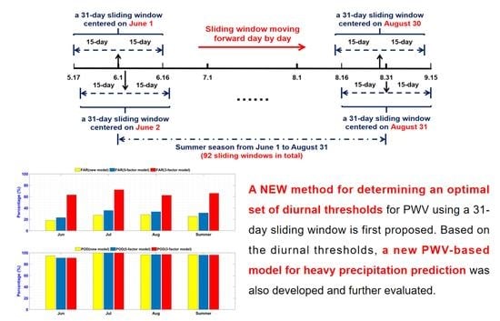
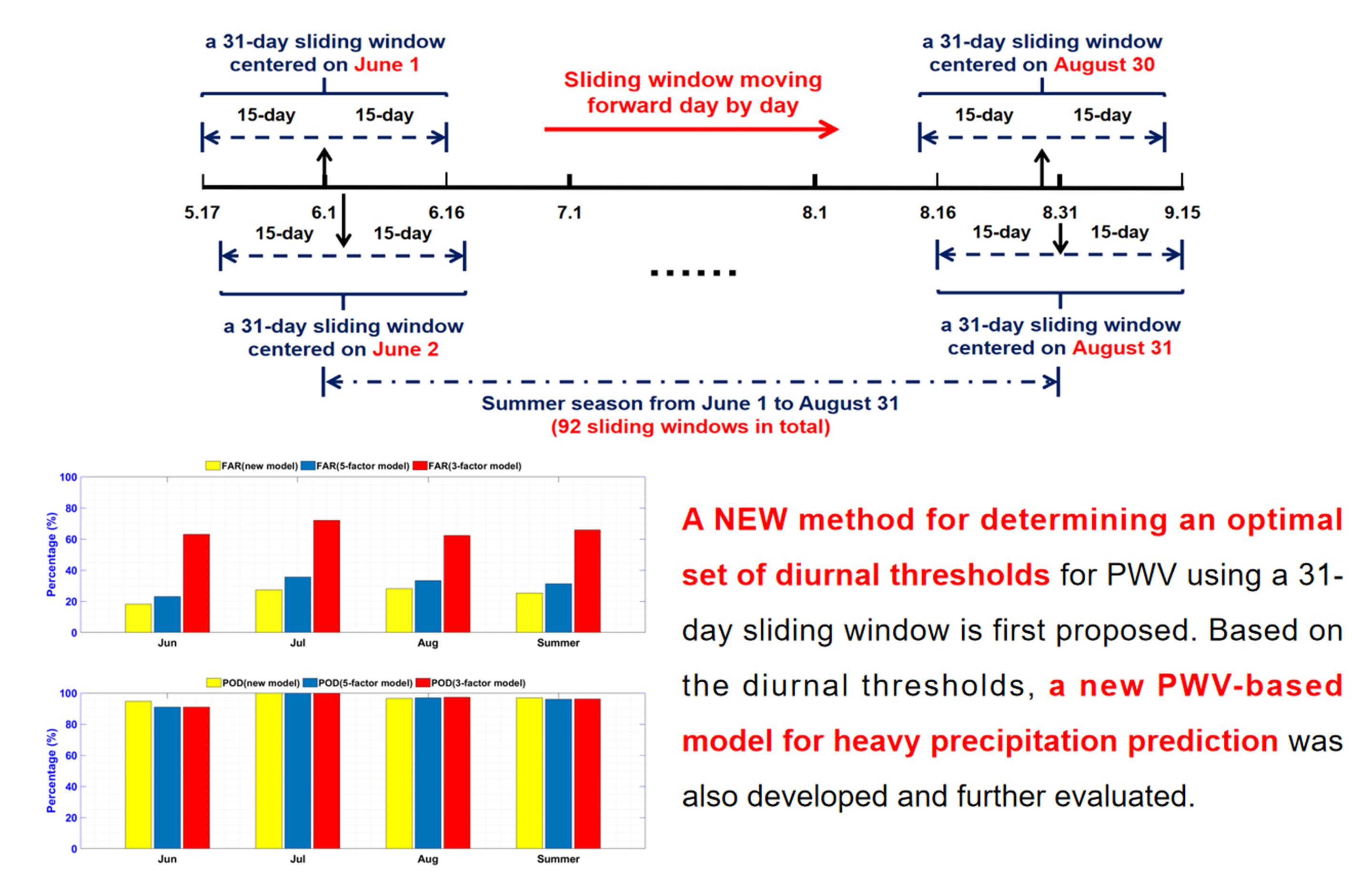
3. New Method for Determining Diurnal Precipitation Thresholds

For any threshold-based precipitation prediction model which uses a set of predefined thresholds for the predictors contained in the model to indicate a rainy condition, its prediction result is largely affected by the selected thresholds. Generally, the larger the threshold value of a predictor, the larger the number of omissive predictions, while the smaller the threshold value of a predictor, the larger the number of misdiagnosis predictions. Therefore, the determination of a reasonable set of thresholds is key to ensure a good performance resulting from a threshold-based model. In this section, based on the CSI, the procedure for determining a set of monthly thresholds, as previously used, is presented. Then, the feasibility of replacing monthly thresholds with diurnal thresholds is analyzed, and a new method for determining an optimal set of diurnal precipitation thresholds is introduced.

3.1. Determining Monthly Precipitation Thresholds Based on CSI

In previous studies, monthly precipitation thresholds for time series of PWV-derived predictors were commonly used, which was effective since the seasonal characteristics and climatic conditions were taken into account. However, these monthly thresholds were often given empirically or selected from a certain value range [15,27]. In our recent study [17], an optimal set of monthly precipitation thresholds were determined based on the CSI, and the threshold for each predictor was unique for each of the three summer months. Generally, the method for the determination of monthly precipitation thresholds for a predictor based on the CSI mainly contained the following steps: (1) A set of candidate threshold values are selected, and the principles for the selection is elaborated in Section 3.3.1; (2) the above candidate threshold values, together with the GNSS-PWV sample data and precipitation records, were used to calculate n11, n12, and n21 in Equation (5) during the period for thresholds determination, e.g., the 8 years from 2010 to 2017 our previous study [17]; (3) the CSI score resulting from each of the candidate thresholds was calculated using Equation (5), and the candidate threshold value that leads to the highest CSI score was determined as the optimal threshold. The flowchart for the procedure of determining threshold value based on CSI is shown in Figure 1, and more information on this can be found in our previous study [17].

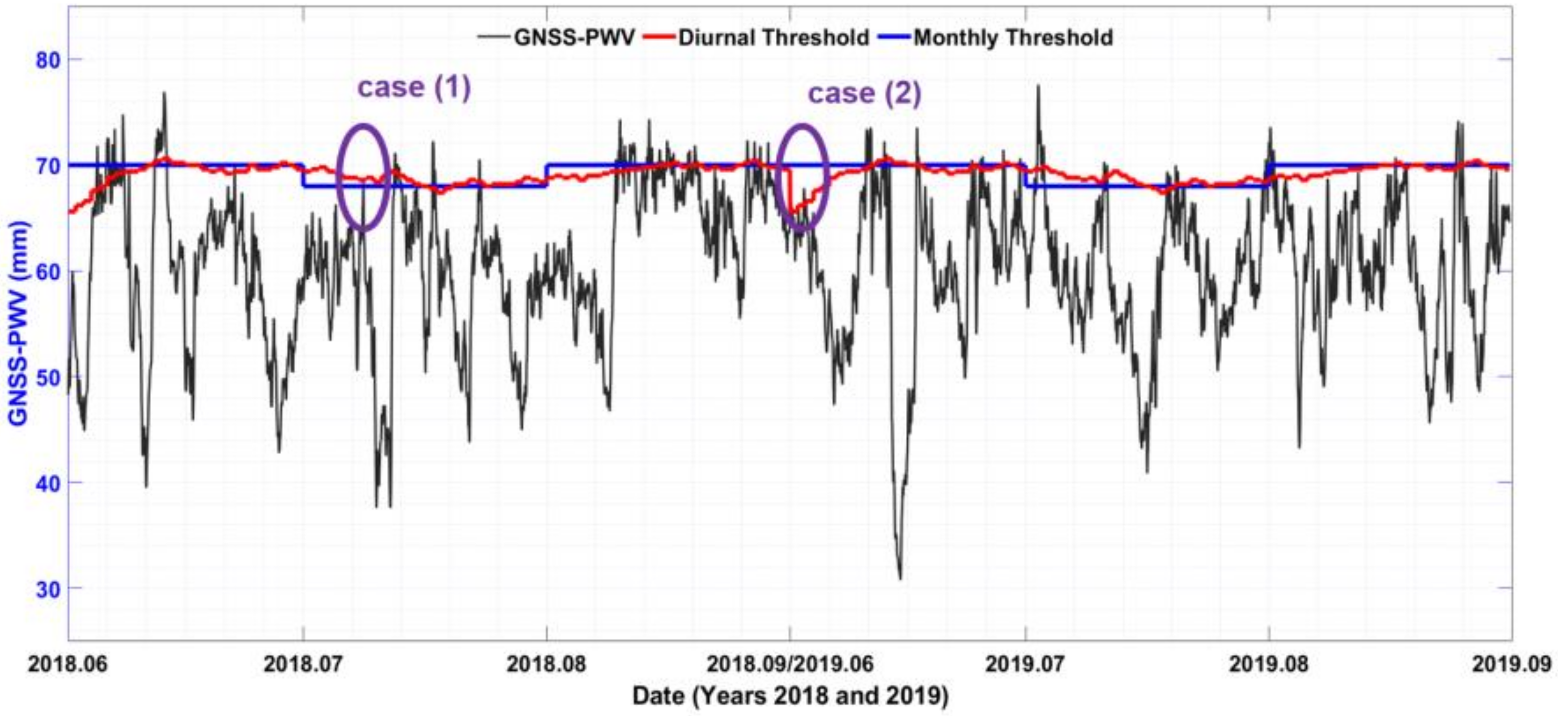
3.2. Rationality of Replacing Monthly Thresholds with Diurnal Thresholds

Although monthly thresholds for threshold-based models have been commonly used in recent studies [15,29,31], due to the monthly thresholds being obtained based on the sample data of the month, the thresholds of a predictor for 2 consecutive months may be significantly different. As stated in Section 3.1, large changes in the threshold values are most likely to be at the beginning of the latter month. Hence, the disadvantage of using monthly thresholds mainly lies in their poor prediction results in the transitional period between two months, i.e., the beginning and the end of a month. This issue may be solved using diurnal thresholds, which means the temporal resolution of the thresholds is improved by about 30 times. From another perspective, the seasonal and diurnal variables of day-of-year (DOY) and hour-of-day (HOD) are also two major parameters, since they reflect the monthly and diurnal variation features of the rapidly changing predictors such as GNSS-PWV [19]. For example, by conducting the principal component analysis, Manandhar et al. [42] found that GNSS-PWV and the variable of DOY are positively correlated, this conclusion was further corroborated in our recent study using a 2-year GNSS-PWV timeseries (see Figure 2 in [17]). In addition, as suggested by Tomassini et al. [43], GNSS observations exhibit an obvious diurnal cycle, meaning these observations are dependent on the variable of HOD. Therefore, these conclusions confirm the rationality of replacing monthly thresholds with diurnal thresholds in a threshold-based model in this study.

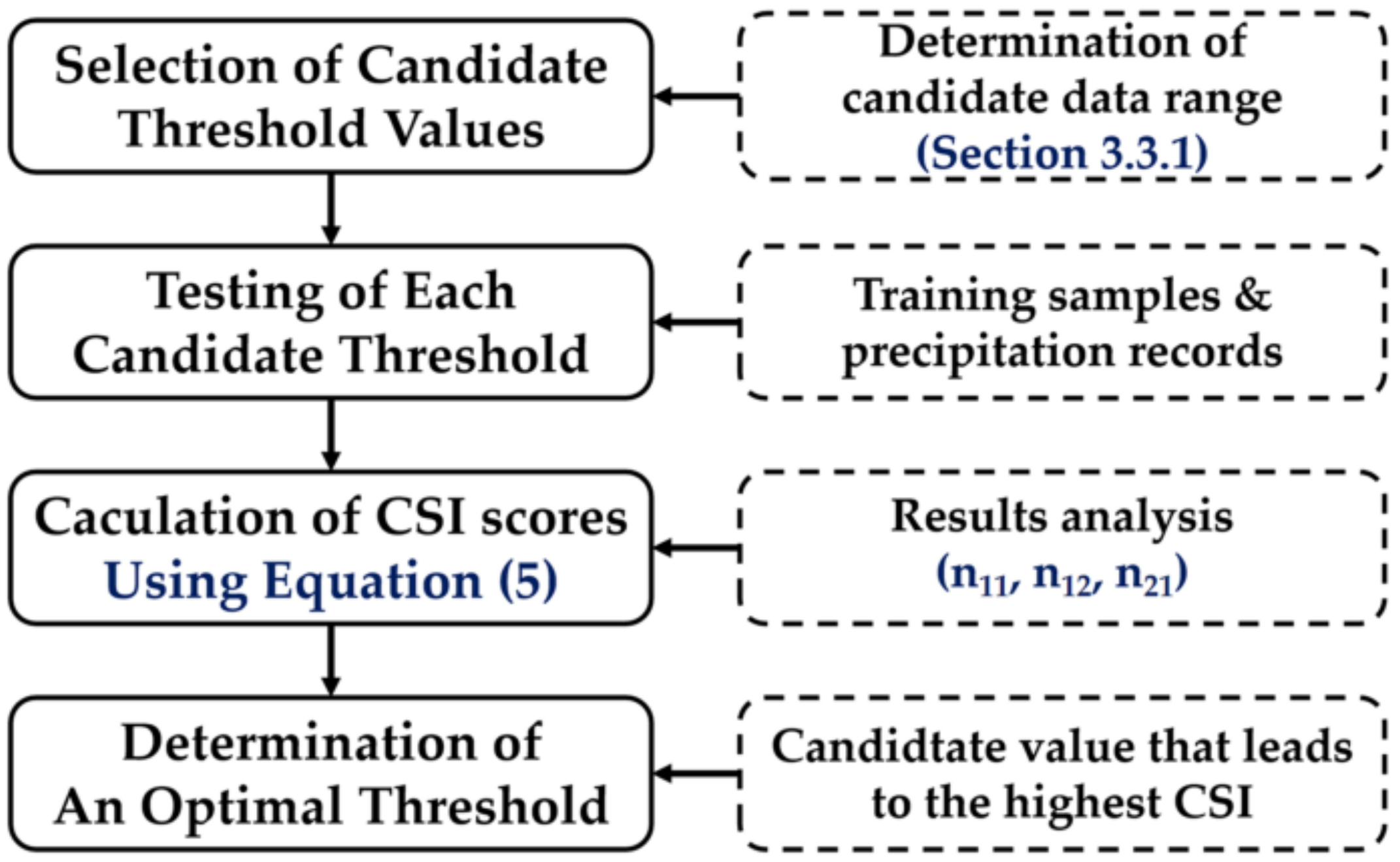
3.3. Determination of Optimal Diurnal Precipitation Thresholds

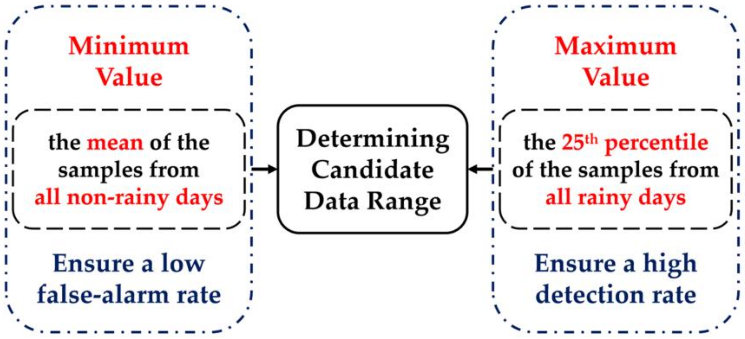
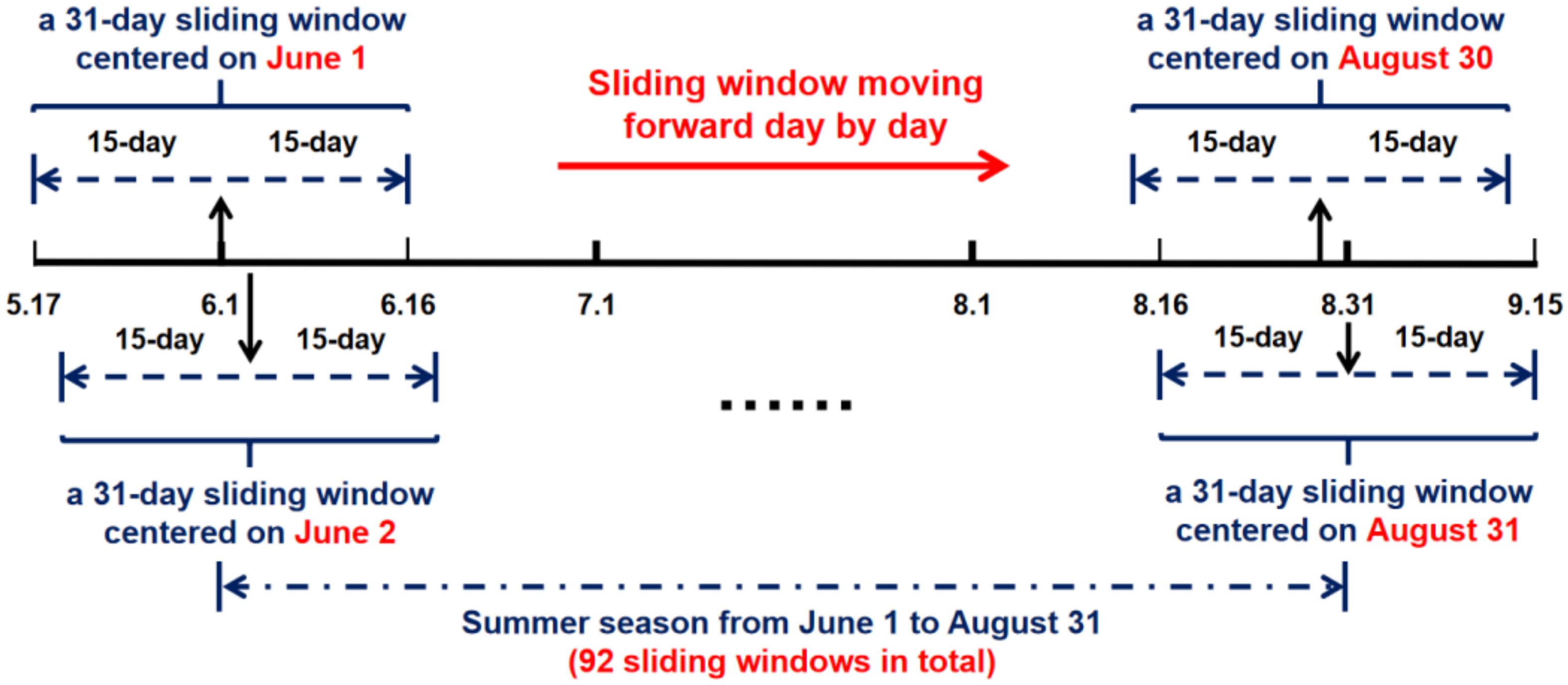
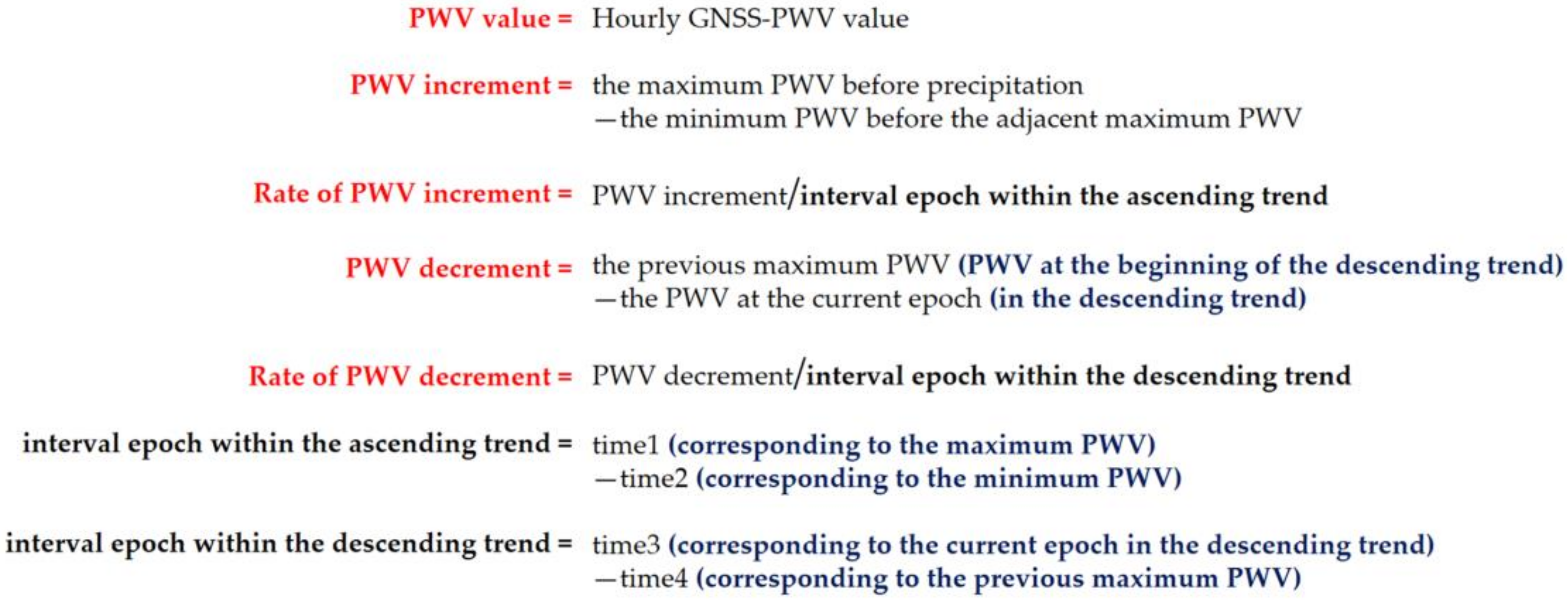
3.3.1. Determining Candidate Data Range

As stated in Section 3.1, prior to the determination of the precipitation threshold for each of the predictors contained in a prediction model, a set of candidate values are selected based on both the samples of the predictor and their corresponding precipitation records over a certain period. The general principles for determining the minimum and maximum of the candidate data range are: (1) To ensure a low FAR score, the minimum is set to the mean of the samples from all non-rainy days in the period; (2) to ensure a high detection rate, i.e., less omissive predictions, the 25th percentile of the samples from all rainy days in the period is set to the maximum [42]. The schematic diagram for determining candidate data range is depicted in Figure 2.

3.3.2. Determining Diurnal Threshold Based on CSI

According to the procedure for determining a precipitation threshold based on the CSI introduced in Section 3.1, the monthly threshold is determined using the sample data of the month studied from a long period, e.g., from several consecutive years. However, for diurnal threshold determination, the size of the samples for a date is too small (only 24 hourly samples from a year). Thus, it cannot reflect any variation trend longer than a day, nor the seasonal/monthly patterns of the predictor. In this study, a new method that uses a 31-day sliding window containing the target date, together with the 15 days before and after the date to determine the diurnal threshold of the date, was proposed. The monthly scale variation of the predictor is also taken into account from the use of the 31-day sliding window, which is mainly based on the finding that a precipitation threshold determined from monthly samples is effective from previous studies [12,29,31]. Figure 3 shows the schematic diagram for the use of the new method to determine the diurnal threshold of a predictor for each of the days during the summer season (from June 1 to August 31, total 92 days), for example.
It can be seen from the left part of the figure that the diurnal threshold for June 1 can be determined based on the principles and procedure stated in Section 3.1 using hourly samples and precipitation records of the 31 days from May 17 to June 16. Then the 31-day sliding window moves 1 day forward, i.e., centered on June 2, and the same procedure was used to determine the diurnal threshold for this date. Finally, the same process was performed continuously in the whole summer season to obtain the diurnal thresholds for all the 92 days.

4. Evaluation of Using New Diurnal Thresholds for Heavy Precipitation Prediction

4.1. Evaluating Predictions from Diurnal and Monthly Thresholds

4.1.1. Comparison of Predictions Resulting from PWV Predictor

In our previous study [17], the performance of applying an optimal set of monthly thresholds determined for the predictor of PWV in each summer months was evaluated. To investigate the improvement of the new diurnal thresholds proposed in this study over the above monthly model, the predictions resulting from the two sets of thresholds are compared in this section. The optimal set of the diurnal thresholds for each day in summer were obtained using the procedure introduced in Section 3.3 and the sample data over the 8-year period 2010–2017 at the HKSC-KP station, which are the same as that used in the monthly model. Figure 4 shows the optimal sets of diurnal (in red) and monthly (in blue) thresholds determined for the prediction of heavy precipitation in the summer season of 2018 and 2019. This is also the reason for the figure also showing the hourly GNSS-PWV (in black) of the 2 years, which were used as the predictor of the models to be compared.
For a quantitative analysis, Table 1 shows the comparison of the fitting and prediction results for the summer months over the periods 2010–2017 and 2018–2019, respectively, by applying the corresponding diurnal and monthly thresholds for the PWV predictor. The diurnal thresholds resulted in a 91.8% seasonal POD score and a 27.4% seasonal FAR score, in comparison with the 87.1% and 43.9% of the monthly thresholds, respectively, meaning a 4.7% improvement in the POD and a 16.5% improvement in the FAR made by replacing the monthly thresholds with the diurnal thresholds. In addition, the predictions in the summer season of 2018 and 2019 together, resulting from the predictor of PWV value using the new diurnal thresholds, indicated an 87.4% seasonal correct detection rate and a 59.5% FAR score compared with the seasonal POD and FAR of 82% and 70.4%, respectively, resulting from monthly thresholds. Thus, a 5.4% improvement in the POD and a 10.9% reduction in the FAR resulted from the use of diurnal thresholds.

4.1.2. Further Analysis

In this section, the improvements by applying the optimal set of diurnal thresholds for the PWV predictor are further analyzed using the two cases highlighted by the purple circles shown in Figure 4 as examples. It is also worth mentioning that, based on the mechanism of using a 31-day sliding window to determine the diurnal threshold for the mid-date of the month with 31 days, i.e., the 16th of the month, the monthly threshold determined in our previous study [17] is exactly the same as the diurnal threshold of the date. For example, the monthly threshold for August is the same as the diurnal threshold for the 16th of the month because both thresholds were determined based on the same 31-day samples in August over the 8-year period studied, which can also be found in Figure 4, as shown by the intersection of the red line (diurnal threshold) and blue line (monthly threshold) on the 16th of August.

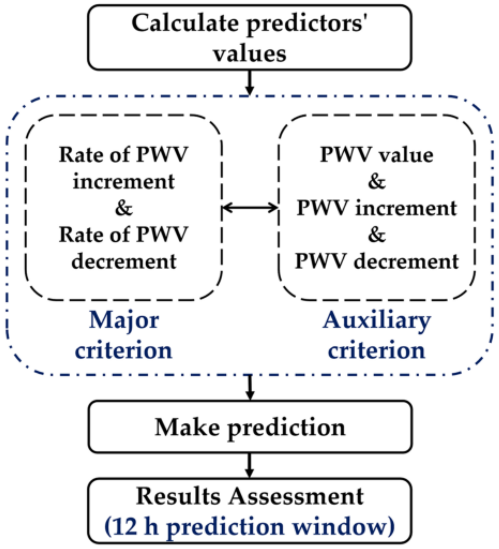
4.2. Developing a New Model Using Diurnal Thresholds for Heavy Precipitation Prediction

In this section, a new GNSS-PWV-based model for heavy precipitation prediction was developed by simply replacing the monthly thresholds used in the five-predictor model proposed in our recent study [17] with an optimal set of diurnal thresholds. Then, the prediction performance resulting from the new model was evaluated by comparison with the results from the existing models.

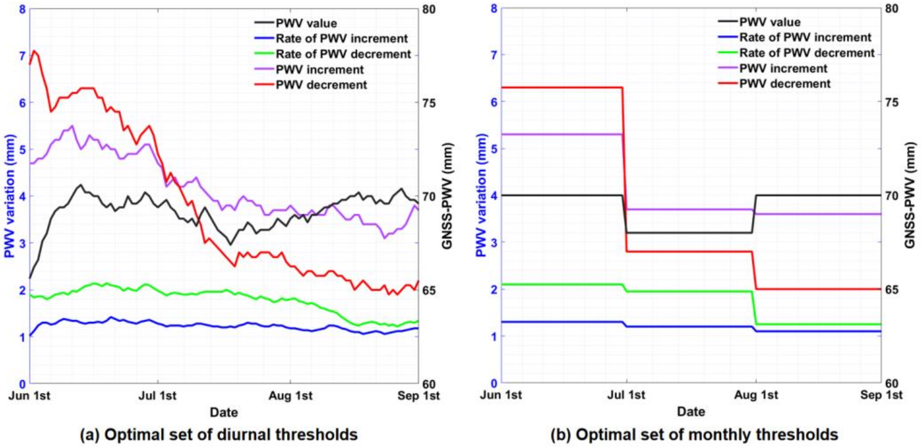
4.2.1. Determining Optimal Diurnal Thresholds
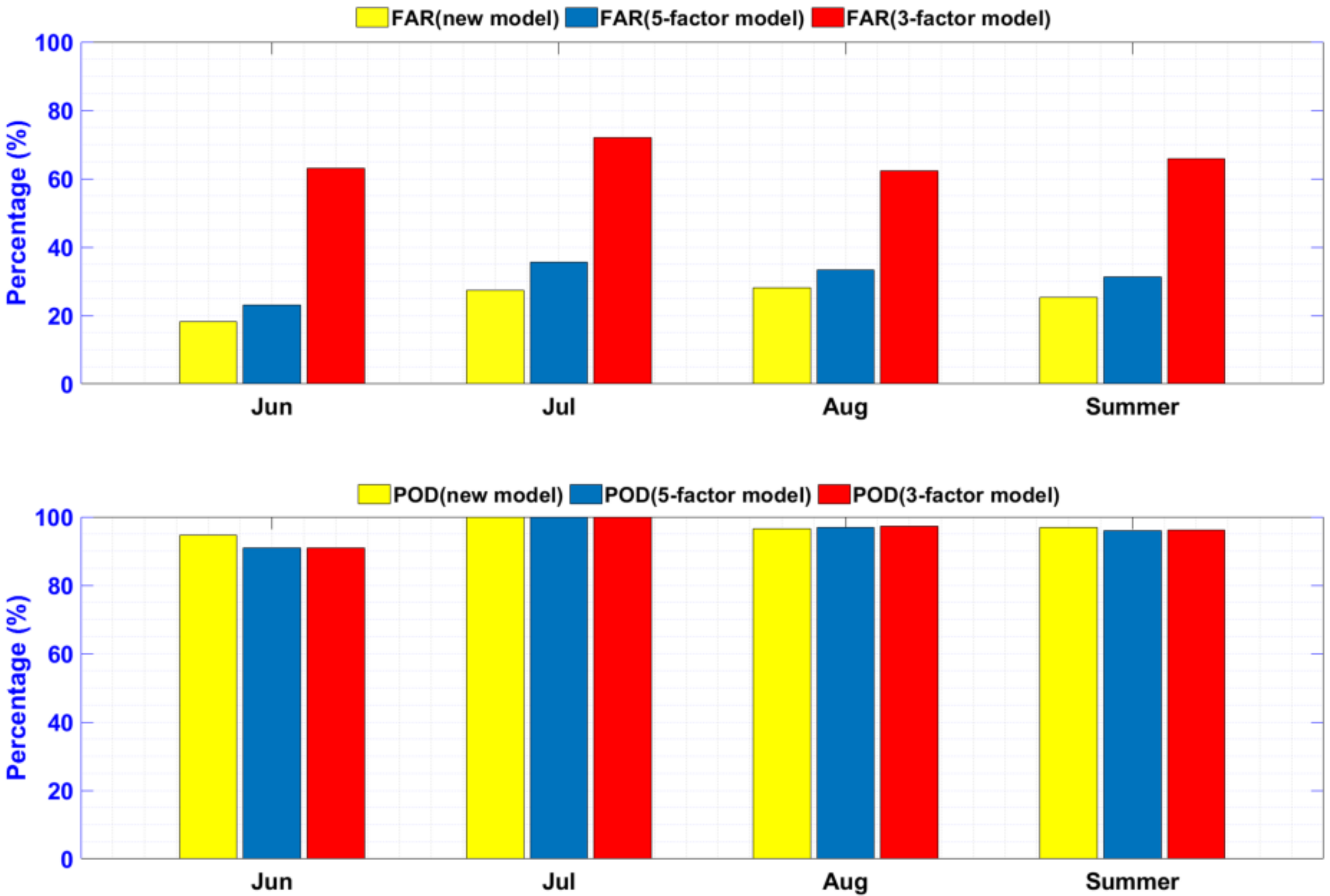
The new model proposed in this study contains the same five predictors (i.e., variables) as the ones used in the monthly model proposed in our previous study [17]. The main difference between the two models is that the former uses diurnal thresholds, while the latter uses monthly thresholds. The definitions of the predictors are shown in Figure 5, as defined in our previous study [17].
The five predictors were all derived from GNSS-PWV timeseries and include the maximum PWV, PWV increment, rate of PWV increment, maximum PWV decrement, and rate of the maximum PWV decrement, which have been proven to be effective in predicting heavy precipitation events. To avoid the non-uniqueness of the values of the three hourly predictors, i.e., PWV, PWV decrement, and rate of PWV decrement, their maximum values in the predefined 12 h sliding prediction window were adopted. As the time period for very short-range forecasting (VSRF) of weather events is in the range of 0–12 h [44], a 12 h sliding prediction window was used in this study. More information about the definitions of the five predictors and the procedure for making a prediction using these predictors can be referred to in our previous study [17].
In Section 3.3, the procedure for determining the optimal diurnal thresholds for the predictor of PWV value in the summer season is presented as an example. The procedure is also applicable to the other four predictors. Therefore, the optimal set of diurnal thresholds for the five predictors for each day in the summer season were determined using the same procedure based on the sample data of PWV timeseries and its corresponding precipitation records at the co-located HKSC-KP stations over the 8-year period of 2010–2017. The optimal set of diurnal thresholds for each day in the summer and the monthly thresholds from our previous study [17] for each summer month are shown in Figure 6 for a comparison. The diurnal thresholds (left) show more fluctuations due to their high temporal resolution and are thus more sensitive to short-term variations of the predictors. The two sets of thresholds were applied to heavy precipitation prediction to test the performance of the new model in comparison with the monthly model in the next section.

4.2.2. Test Results

As stated in Section 4.2.1, the criteria determined for a prediction based on the five predictors are the same as the ones used in our previous study [17], in which the combination of the rate of PWV increment and rate of the maximum PWV decrement was defined as the major criterion, and the other three predictors were defined as the group of auxiliary criterion. Then, based on the above criteria, the prediction results were validated using the precipitation records in the predefined prediction window of the next 12 h as the reference. The flowchart for model testing is shown in Figure 7.
To make a more general comparison, based on the same test data in the 2-year period of 2018−2019, the performances of the new model for each summer month and the summer season were compared with that resulting from the existing five-factor model [17] and three-factor model [15] using the monthly thresholds. Table 2 lists the predictions resulting from the three models, and the CSI, POD, and FAR scores (the last three columns in Table 2) are shown in Figure 8 merely for a clear comparison.
It is evident from Figure 8 and the bold figures (the “Summer” rows) in Table 2 that the new model reduced the seasonal FAR score by 6.1% and 40.5% compared with the five-factor model and the three-factor model, respectively. Although the seasonal POD scores resulting from these models were at a comparable level (from 95.9% to 96.9%), the improvements of 1.0% and 0.7% in the POD were also made by the new model in comparison to the five-factor model and three-factor model. respectively. Furthermore, it can be seen from the statistics of CSI scores resulting from these models that the new model clearly outperformed the other models in each summer month and the whole summer season. More specifically, comparing with the five-factor model, the use of diurnal thresholds in the new model effectively reduced not only the number of misdiagnosis predictions (21 vs. 32) but also the number of omissive predictions (2 vs. 3). From the perspective of the results of the mean lead times, which are the mean values of the lead times for all those correctly predicted events made by these models, the statistics of 4.86 h from the new model and 5.15 h from the five-factor model suggest that both were at a comparable level. Overall, the considerable improvements in prediction results made by diurnal thresholds, instead of monthly thresholds, for the predictors derived from GNSS-PWV timeseries suggest, again, that it is more rational to apply diurnal thresholds for better prediction results.

5. Discussion

The potential of using GNSS-PWV for forecasting and nowcasting severe weather events like heavy precipitation has been actively researched in many regions in recent years. A practical approach is to provide a threshold value that can trigger an extreme weather event, i.e., the threshold-based model adopted in this study. Comparing with the operational NWP model, which has a solid physical basis and incorporates a lot of meteorological variables, the threshold-based model is more likely to result in more unstable prediction performances (more misdiagnosis and omissive predictions), since the conditions of dynamic (wind, convergence) are often overlooked by the model based on limited number of variables/predictors (e.g., GNSS-PWV in this study). However, the potential of using the threshold-based model has clearly been demonstrated in recent studies due to its high spatiotemporal resolutions which can be regarded as a complementary method to the operational models, especially for the nowcasting of severe weather events.
For a threshold-based model used to predict heavy precipitation, the determination of a set of appropriate thresholds is important for good prediction results. Generally, an overlarge threshold is likely to result in more omissive predictions, while a rather small threshold often leads to more misdiagnosis predictions. In previous studies, empirical thresholds, which were often given within a certain data range, were simply used without justification. In this study, the widely accepted criterion of the CSI, which was obtained from sufficient amount of sample data, was used to determine an optimal set of thresholds, and each predictor has a unique threshold value for a certain time-length, e.g., monthly or diurnal threshold. Although monthly thresholds have been widely used in recent studies, the main disadvantage lies in their poor prediction results in the transitional period between two consecutive months. Hence, this study validated the rationality of replacing monthly thresholds with diurnal thresholds and proposed to use the sample data within a 31-day sliding window to determine an optimal set of diurnal thresholds for a threshold-based model. Both the monthly and diurnal variations of the predictors were taken into account in the newly proposed diurnal thresholds.
Furthermore, it is noted from Table 2 that the POD scores resulting from the monthly models, i.e., the five-factor model and the three-factor model, were higher than that of the new model in the month of August. This phenomenon is mainly attributed to the computing mechanism of the POD using Equation (6), i.e., with the same number of omissive predictions, greater number of correct predictions, and higher POD score. In August, only one heavy precipitation event failed to be detected by the three models. However, before those correctly predicted events, predictions of “heavy precipitation” were made by more epochs in the 12 h prediction window from the monthly models. Hence, the POD scores resulting from the monthly models were higher. From the perspective of the CSI score, which is a function of both POD and FAR according to Equations (5)–(7), it is obvious that the CSI scores resulting from the new model were higher than that of the monthly models in each summer month, meaning the new model outperformed the other models. This conclusion further corroborates the effectiveness of CSI, which is taken as the major criterion to determine precipitation threshold.

6. Conclusions

In this study, for heavy precipitation prediction, a new method using GNSS-PWV sample data within a 31-day sliding window to determine an optimal set of diurnal thresholds for predictors derived from GNSS-PWV timeseries was proposed for the first time. Based on an existing five-predictor PWV-based model that was based on monthly thresholds to make predictions for heavy precipitation events, a new model based on diurnal thresholds was developed. The optimal set of diurnal thresholds for the five predictors were determined using the hourly GNSS-PWV and precipitation records for the summer over the 8-year period from 2010 to 2017 at the co-located HKSC-KP stations in Hong Kong. The new model was evaluated by comparing its prediction results for the summer in 2018 and 2019 against the hourly precipitation records in the same duration. Results showed that the seasonal FAR score resulting from the new model was reduced from 31.4% to 25.3%, and 96.9% of heavy precipitation events were correctly predicted with a lead time of 4.86 h. These results suggest that the inclusion of diurnal thresholds can significantly improve the prediction performance.
To further improve the performance of heavy precipitation prediction, our future work will focus on applying diurnal thresholds to other predictors that are potentially contained in a new model and that are derived from various types of atmospheric data such as ZTD. In addition, the incorporation of other useful meteorological variables using the machine learning and data assimilation techniques will also be investigated.

Author Contributions

Conceptualization, H.L.; Formal analysis, H.L. and X.W.; Funding acquisition, H.L., X.W. and K.Z.; Methodology, H.L., X.W. and K.Z.; Resources, X.W., E.F., C.Q., J.Z. and L.L.; Software, H.L.; Supervision, X.W., S.W., K.Z. and Y.X.; Validation, H.L., X.W. and S.W.; Writing–original draft, H.L.; Writing–review & editing, X.W., S.W. and K.Z. All authors have read and agreed to the published version of the manuscript.

Funding

This research was supported in part by the China Natural Science Funds under Grants 41904033, 41730109, in part by the Strategic Priority Research Program of the Chinese Academy of Sciences (CAS) under Grant XDA17010304, in part by the CAS Pioneer Hundred Talents Program, National Key Research and Development Plan, under Grant 2016YFB0501405, in part by the Natural Science Foundation of Shandong Province under Grant ZR2019MD005, and in part by the Postgraduate Research & Practice Innovation Program of Jiangsu Province under Grant KYCX20_1835.

Data Availability Statement

Not applicable.

Acknowledgments

The authors would like to thank the IGS for providing precise GPS data, the Hong Kong Observation for providing hourly precipitation data.

Conflicts of Interest

The authors declare no conflict of interest.

References

  1. Bevis, M.; Businger, S.; Herring, T.; Rocken, C.; Anthes, R.; Ware, R. GPS Meteorology: Remote Sensing of Atmospheric Water Vapor Using the Global Positioning System. J. Geophys. Res. Atmos. 1992, 97, 15787–15801. [Google Scholar] [CrossRef]
  2. Bonafoni, S.; Biondi, R.; Brenot, H.; Anthes, R. Radio occultation and ground-based GNSS products for observing, understanding and predicting extreme events: A review. Atmos. Res. 2019, 230, 104624. [Google Scholar] [CrossRef]
  3. Cardellach, E.; Oliveras, S.; Rius, A.; Tomás, S.; Ao, C.O.; Franklin, G.W.; Iijima, B.A.; Kuang, D.; Meehan, T.K.; Padullés, R.; et al. Sensing Heavy Precipitation With GNSS Polarimetric Radio Occultations. Geophys. Res. Lett. 2019, 46, 1024–1031. [Google Scholar] [CrossRef] [Green Version]
  4. Gao, F.; Xu, T.; Wang, N.; Jiang, C.; Du, Y.; Nie, W.; Xu, G. Spatiotemporal evaluation of GNSS-R based on future fully operational global multi-GNSS and Eight-LEO constellations. Remote Sens. 2018, 10, 67. [Google Scholar] [CrossRef] [Green Version]
  5. Baker, H.C.; Dodson, A.H.; Penna, N.T.; Higgins, M.; Offiler, D. Ground-based GPS water vapour estimation: Potential for meteorological forecasting. J. Atmos. Sol. Terr. Phys. 2001, 63, 1305–1314. [Google Scholar] [CrossRef]
  6. Gradinarsky, L.P.; Johansson, J.; Bouma, H.; Scherneck, H.-G.; Elgered, G. Climate monitoring using GPS. Phys. Chem. Earth 2002, 27, 335–340. [Google Scholar] [CrossRef]
  7. Zhang, K.; Manning, T.; Wu, S.; Rohm, W.; Silcock, D.; Choy, S. Capturing the Signature of Severe Weather Events in Australia Using GPS Measurements. IEEE J. Sel. Top. Appl. Earth Obs. Remote Sen. 2015, 8, 1839–1847. [Google Scholar] [CrossRef]
  8. Zhao, Q.; Liu, Y.; Yao, W.; Yao, Y. Hourly rainfall forecast model using supervised learning algorithm. IEEE Tran. Geosci. Remote Sens. 2021. [Google Scholar] [CrossRef]
  9. Rohm, W.; Yuan, Y.; Biadeglgne, B.; Zhang, K.; Le Marshall, J. Ground-based GNSS ZTD/IWV estimation system for numerical weather prediction in challenging weather conditions. Atmos. Res. 2013, 138, 414–426. [Google Scholar] [CrossRef]
  10. Wang, X.; Zhang, K.; Wu, S.; Li, Z.; Cheng, Y.; Li, L.; Yuan, H. The correlation between GNSS-derived precipitable water vapor and sea surface temperature and its responses to El Niño–Southern Oscillation. Remote Sens. Environ. 2018, 216, 1–12. [Google Scholar] [CrossRef]
  11. Hagemann, S.; Bengtsson, L.; Gendt, G. On the determination of atmospheric water vapor from GPS measurements. J. Geophys. Res. 2003, 108, D214678. [Google Scholar]
  12. Jin, S.; Park, J.; Cho, J.-H.; Park, P.-H. Seasonal variability of GPS-derived zenith tropospheric delay (1994–2006) and climate implications. J. Geophys. Res. 2007, 112, D09110. [Google Scholar] [CrossRef]
  13. Nilsson, T.; Elgered, G. Long-term trends in the atmospheric water vapor content estimated from ground-based GPS data. J. Geophys. Res. 2008, 113, D19101. [Google Scholar] [CrossRef] [Green Version]
  14. Wang, X.; Zhang, K.; Wu, S.; Fan, S.; Cheng, Y. Water vapor-weighted mean temperature and its impact on the determination of precipitable water vapor and its linear trend. J. Geophys. Res. Atmos. 2016, 121, 833–852. [Google Scholar] [CrossRef]
  15. Yao, Y.; Shan, L.; Zhao, Q. Establishing a method of short-term rainfall forecasting based on GNSS-derived PWV and its application. Sci. Rep. 2017, 7, 1–11. [Google Scholar] [CrossRef]
  16. Zhao, Q.; Yao, Y.; Yao, W. GPS-based PWV for precipitation forecasting and its application to a typhoon event. J. Atmos. Sol. Terr. Phy. 2018, 167, 124–133. [Google Scholar] [CrossRef]
  17. Li, H.; Wang, X.; Wu, S.; Zhang, K.; Chen, X.; Qiu, C.; Zhang, S.; Zhang, J.; Xie, M.; Li, L. Development of an Improved Model for Prediction of Short-Term Heavy Precipitation Based on GNSS-Derived PWV. Remote Sens. 2020, 12, 4101. [Google Scholar] [CrossRef]
  18. Sangiorgio, M.; Barindelli, S.; Biondi, R.; Solazzo, E.; Realini, E.; Venuti, G.; Guariso, G. Improved extreme rainfall events forecasting using neural networks and water vapor measures. In Proceedings of the 6th International conference on Time Series and Forecasting (ITISE-2019), Granada, Spain, 25–27 September 2019; pp. 820–826. [Google Scholar]
  19. Liu, Y.; Zhao, Q.; Yao, W.; Ma, X.; Yao, Y.; Liu, L. Short-term rainfall forecast model based on the improved Bp–nn algorithm. Sci. Rep. 2019, 9, 1–12. [Google Scholar] [CrossRef]
  20. Benevides, P.; Catalao, J.; Nico, G. Neural network approach to forecast hourly intense rainfall using GNSS precipitable water vapor and meteorological sensors. Remote Sens. 2019, 11, 966. [Google Scholar] [CrossRef] [Green Version]
  21. Manandhar, S.; Dev, S.; Lee, Y.H.; Meng, Y.S.; Winkler, S. A data-driven approach for accurate rainfall prediction. IEEE Tran. Geosci. Remote Sens. 2019, 57, 9323–9331. [Google Scholar] [CrossRef] [Green Version]
  22. Kuo, Y.; Guo, Y.; Westwater, E. Assimilation of precipitable water measurements into a mesoscale numerical model. Mon. Weather Rev. 1993, 121, 1215–1238. [Google Scholar] [CrossRef] [Green Version]
  23. Smith, T.; Benjamin, S.; Gutman, S.; Sahm, S. Short-range forecast impact from assimilation of GPS-IPW observations into the Rapid Update Cycle. Mon. Weather Rev. 2007, 135, 2914–2930. [Google Scholar] [CrossRef]
  24. Rohm, W.; Guzikowski, J.; Wilgan, K.; Kryza, M. 4DVAR assimilation of GNSS zenith path delays and precipitable water into a numerical weather prediction model WRF. Atmos. Meas. Tech. 2019, 12, 345–361. [Google Scholar] [CrossRef] [Green Version]
  25. Benjamin, S.G.; Weygandt, S.S.; Brown, J.M.; Hu, M.; Alexander, C.R.; Smirnova, T.G.; Olson, J.B.; James, E.P.; Dowell, D.C.; Grell, G.A.; et al. A North American Hourly Assimilation and Model Forecast Cycle: The Rapid Refresh. Mon. Weather Rev. 2016, 144, 1669–1694. [Google Scholar] [CrossRef]
  26. Shaffie, S.; Mozaffari, G.; Khosravi, Y. Determination of extreme precipitation threshold and analysis of its effective patterns (case study: West of Iran). Nat. Hazards 2019, 99, 857–878. [Google Scholar] [CrossRef]
  27. Benevides, P.; Catalao, J.; Miranda, P. On the inclusion of GPS precipitable water vapour in the nowcasting of rainfall. Nat. Hazard Earth Syst. 2015, 15, 2605–2616. [Google Scholar] [CrossRef] [Green Version]
  28. Yeh, T.K.; Shih, H.C.; Wang, C.S.; Choy, S.; Chen, C.H.; Hong, J.S. Determining the precipitable water vapor thresholds under different rainfall strengths in Taiwan. Adv. Space Res. 2018, 61, 941–950. [Google Scholar] [CrossRef]
  29. Zhao, Q.; Liu, Y.; Ma, X.; Yao, W.; Yao, Y.; Li, X. An Improved Rainfall Forecasting Model Based on GNSS Observations. IEEE Trans. Geosci. Remote Sens. 2020, 58, 4891–4900. [Google Scholar] [CrossRef]
  30. Hubert, M.; Vandervieren, E. An adjusted boxplot for skewed distributions. Comput. Statist. Data Anal. 2008, 52, 5186–5201. [Google Scholar] [CrossRef]
  31. Shi, J.; Xu, C.; Guo, J.; Gao, Y. Real-time GPS precise point positioning-based precipitable water vapor estimation for rainfall monitoring and forecasting. IEEE Trans. Geosci. Remote Sens. 2015, 53, 3452–3459. [Google Scholar]
  32. Jin, S.; Li, Z.; Cho, J. Integrated water vapor field and multiscale variations over China from GPS measurements. J. Appl. Meteorol. Clim. 2008, 47, 3008–3015. [Google Scholar] [CrossRef]
  33. Manandhar, S.; Lee, Y.H.; Meng, Y.S. GPS-PWV Based Improved Long-Term Rainfall Prediction Algorithm for Tropical Regions. Remote Sens. 2019, 11, 2643. [Google Scholar] [CrossRef] [Green Version]
  34. Ding, J. Review of Weather Prediction Verifying Techniques. J. Nanjing Inst. Meteorol. 1995, 18, 143–150. [Google Scholar]
  35. Böhm, J.; Werl, B.; Schuh, H. Troposphere mapping functions for GPS and very long baseline interferometry from European Centre for Medium-Range Weather Forecasts operational analysis data. J. Geophys. Res. Solid Earth 2006, 111. [Google Scholar] [CrossRef]
  36. Saastamoinen, J. Atmospheric Correction for the Troposphere and the Stratosphere in Radio Ranging of Satellites. Geophys. Monogr. 1972, 15, 247–251. [Google Scholar]
  37. Bevis, M.; Businger, S.; Chiswell, S.; Herring, T.; Anthes, R.; Rocken, C.; Ware, R. GPS Meteorology: Mapping Zenith Wet Delays onto Precipitable Water. J. Appl. Meteorol. 1994, 33, 379–386. [Google Scholar] [CrossRef]
  38. Chen, Y. Inversing the content of vapor in atmosphere by GPS observations. Mod. Surv. Mapp. 2005, 28, 3–6. [Google Scholar]
  39. Donaldson, R.; Dyer, R.; Kraus, M. Objective evaluator of techniques for predicting severe weather events. Bull. Amer. Meteorol. Soc. 1975, 56, 755. [Google Scholar]
  40. Gilleland, E.; Ahijevch, D.; Brown, B.; Casati, B.; Ebert, E. Intercomparison of Spatial Forecast Verification Methods. Weather Forecast. 2009, 24, 1416–1430. [Google Scholar] [CrossRef]
  41. Doswell Iii, C.; Davies-Jones, R.; Keller, D. On Summary Measures of Skill in Rare Event Forecasting Based on Contingency Tables. Weather Forecast. 1990, 5, 576–585. [Google Scholar] [CrossRef] [Green Version]
  42. Manandhar, S.; Dev, S.; Lee, Y.; Winkler, S.; Meng, Y. Systematic study of weather variables for rainfall detection. In Proceedings of the 2018 IEEE International Geoscience and Remote Sensing Symposium (IGARSS 2018), Valencia, Spain, 22–27 July 2018; pp. 3027–3030. [Google Scholar]
  43. Tomassini, M.; Gendt, G.; Dick, G.; Ramatschi, M.; Schraff, C. Monitoring of integrated water vapour from ground-based GPS observations and their assimilation in a limited-area NWP model. Phys. Chem. Earth 2002, 27, 341–346. [Google Scholar] [CrossRef]
  44. WMO. Guidelines for Nowcasting Techniques; No. 1198; World Meteorological Organization: Geneva, Switzerland, 2017; Available online: https://library.wmo.int/doc_num.php?explnum_id=3795 (accessed on 25 March 2021).
Figure 1. Flowchart for the procedure of determining threshold value based on the critical success index (CSI).
Remotesensing 13 01390 g001
Figure 2. Schematic diagram for determining candidate data range.
Remotesensing 13 01390 g002
Figure 3. Schematic diagram of using the new method to determine the diurnal threshold for each of the days during the summer season.
Remotesensing 13 01390 g003
Figure 4. Timeseries of hourly Global Navigation Satellite System-precipitable water vapor (GNSS-PWV) (black), and diurnal (red) and monthly (blue) precipitation thresholds determined for the prediction for the summer season in 2018 and 2019.
Remotesensing 13 01390 g004
Figure 5. Definitions of the five predictors used in this study.
Remotesensing 13 01390 g005
Figure 6. Optimal set of diurnal (a) and monthly (b) thresholds of five predictors determined for the summer season using sample data in the month over the period 2010–2017 from the co-located HKSC-KP stations.
Remotesensing 13 01390 g006
Figure 7. Flowchart for model testing.
Remotesensing 13 01390 g007
Figure 8. Comparison of the probability of detection (POD) and high false alarm rates (FAR) scores of predictions from the new model and the monthly models (five-factor model and three-factor model).
Remotesensing 13 01390 g008
Table 1. Comparison of the fitting (2010–2017) and prediction (2018–2019) results for the summer season applying the diurnal and monthly thresholds for the PWV predictor.
Result TypeThreshold TypeMonthNo. of Correct
Predictions (n11)
No. of Misdiagnosis
Predictions (n12)
No. of Omissive
Predictions (n21)
POD (%)FAR (%)
Fitting ResultsMonthly threshold Jun4014981.625.9
Jul5648788.946.2
Aug7370989.049.0
Summer1691322587.143.9
Diurnal thresholdJun4712688.720.3
Jul4119295.331.7
Aug5824592.129.3
Summer146551391.827.4
Prediction ResultsMonthly threshold Jun2353679.369.7
Jul2746584.463.0
Aug3276782.170.4
Summer82175188268.1
Diurnal thresholdJun2647583.964.4
Jul2333388.558.9
Aug3442489.555.3
Summer831221287.459.5
Table 2. Comparison of predictions resulting from the new model and the monthly models (five-factor model and three-factor model) for each summer month and summer season in the 2-year period of 2018–2019.
Model TypeMonthNo. of Correct
Predictions (n11)
No. of Misdiagnosis
Predictions (n12)
No. of Omissive
Predictions (n21)
CSI (%)POD (%)FAR (%)
Monthly model
(3-factor)
Jun2034235.790.963.0
Jul2154028.010072.0
Aug3558137.297.262.4
Summer76146333.896.265.8
Monthly model
(5-factor)
Jun206271.490.923.1
Jul1810064.310035.7
Aug3216165.397.033.3
Summer7032366.795.931.4
New modelJun184178.394.718.2
Jul166072.710027.3
Aug2811170.096.628.2
Summer6221272.996.925.3
Publisher’s Note: MDPI stays neutral with regard to jurisdictional claims in published maps and institutional affiliations.

