
Graph Convolutional Networks by Architecture Search for PolSAR Image Classification
by
 , ,
, ,
Hongying Liu
1 ,
,
Derong Xu
1,
Tianwen Zhu
1,
Fanhua Shang
1,* ,
,
Yuanyuan Liu
1,
Jianhua Lu
2 and
Ri Yang
2 1
Key Laboratory of Intelligent Perception and Image Understanding of Ministry of Education, Xidian University, Xi’an 710071, China
2
Xi’an Satellite Control Center, Xi’an 710043, China
*
Author to whom correspondence should be addressed.
Remote Sens. 2021, 13(7), 1404; https://0-doi-org.brum.beds.ac.uk/10.3390/rs13071404
Submission received: 21 February 2021
/
Revised: 29 March 2021
/
Accepted: 30 March 2021
/
Published: 6 April 2021
(This article belongs to the Section AI Remote Sensing)
Abstract
:Classification of polarimetric synthetic aperture radar (PolSAR) images has achieved good results due to the excellent fitting ability of neural networks with a large number of training samples. However, the performance of most convolutional neural networks (CNNs) degrades dramatically when only a few labeled training samples are available. As one well-known class of semi-supervised learning methods, graph convolutional networks (GCNs) have gained much attention recently to address the classification problem with only a few labeled samples. As the number of layers grows in the network, the parameters dramatically increase. It is challenging to determine an optimal architecture manually. In this paper, we propose a neural architecture search method based GCN (ASGCN) for the classification of PolSAR images. We construct a novel graph whose nodes combines both the physical features and spatial relations between pixels or samples to represent the image. Then we build a new searching space whose components are empirically selected from some graph neural networks for architecture search and develop the differentiable architecture search method to construction our ASGCN. Moreover, to address the training of large-scale images, we present a new weighted mini-batch algorithm to reduce the computing memory consumption and ensure the balance of sample distribution, and also analyze and compare with other similar training strategies. Experiments on several real-world PolSAR datasets show that our method has improved the overall accuracy as much as 3.76% than state-of-the-art methods.
1. Introduction
Polarimetric synthetic aperture radar (PolSAR) data has wide applications in agriculture, forestry, geology, ocean, etc. [1,2,3,4]. In agriculture, PolSAR data are used for identification crop species, monitoring crop growth and assessment land conditions [5]. In forestry, PolSAR data are adopted to monitor the fire and excessive logging as well as estimate the biomass in forest [6]. In geology, PolSAR data are employed to analyze information such as geological structure, mineral distribution, surface roughness, ground coverage, and soil moisture [7]. Polarimetric SAR data classification is the key for data interpretation and one of the important research for PolSAR data processing.
The current classification methods for PolSAR generally can be categorized as the unsupervised, supervised, and semi-supervised learning. The unsupervised method does not need to use labeled samples for training, while the supervised classification method utilizes a certain number of labeled samples to train a classifier, and then classify the unlabeled samples. More recently, the semi-supervised learning has attracted increasing attention. It uses a few labeled samples and a large number of unlabeled samples for classification. With the development of deep learning, the networks with more complex architectures can be designed for classification, and have improved classification performance in the case of only a few labeled samples.
As one of the semi-supervised learning methods, the graph convolutional network (GCN) [8,9] is graph structured learning network, and it has wide application in modeling social networks, segmentation large point clouds, and predicting biomolecular structure. In SemiGCN [9], a graph using binary weights is constructed and then several graph convolutional layers are stacked following by a Softmax function, in which the labels propagate to the unlabeled samples for semi-supervised classification. However, the above mentioned works mainly construct their networks manually. They need to design delicate networks for the given data. As it is known, the performance of deep learning algorithms heavily depends on the architectures of neural networks, which costs considerable effort for experts to select and determine a suitable one for a specific application. The network with an optimal architecture is still uncovered, which is also challenging. In this paper, inspired by the success of Neural Architecture Search (NAS) [10], we propose a new graph convolutional network based on architecture search, called ASGCN, for PolSAR classification. We first build a fine-grained graph with varying weights, and then propose a weight-based mini-batch strategy to partition the graph into subgraphs. Moreover, we construct a searching space for the architecture search of ASGCN, and utilize the subgraphs to search an optimal architecture for classification.
The main contributions of this paper can be summarized as follows: We propose a novel ASGCN based on architecture search to automatically find the optimal network structure for feature learning and classification. A new search space is constructed for our ASGCN, which provides a variety of possibilities for model selection. Then a new training method is also presented, which can ensure the balance and diversity of sample distribution, and decrease memory and computational costs.
2. Background
2.1. The Classification Methods of PolSAR Data
Most of the classification methods are unsupervised in the early years. Researchers rely on analyzing scattering matrix and covariance matrix for classification. For example, in [11], the authors perform polarimetric decomposition to yield the H/a components and then utilize a complex Wishart classifier. In [12], the pixels are divided into different scattering categories based on Freeman and Durden decomposition [13], and then fine-grained classification is achieved by applying the Wishart classifier iteratively. Recently the statistical analyzing and machine learning methods are applied to categorization. For instance, the minimum stochastic distance is compared and analyzed in [14]. The Fuzzy K-means algorithm is employed for classification [15,16]. In [17,18,19,20,21], the authors calculate statistics of the covariance matrix for classification pixels. In [22], a new super-pixel generation method named as fuzzy super-pixel (FS) is proposed for PolSAR image classification. The deep learning-based methods have also been presented, for instance, in Wishart Deep Belief Network (W-DBN) [23], the restricted Boltzman machines are stacked to model PolSAR data and for classification.
The classical supervised algorithms include: support vector machine (SVM) [24,25], sparse coding classifiers, boosting, and random forest [26,27,28], multi-objective optimization-based approach [29]. Recently, the convolutional neural networks (CNNs) and their variants are applied for feature extraction and classification in [30,31,32].
In semi-supervised learning, the model uses a few labeled samples and a large number of unlabeled samples for classification. In [33], the authors proposed a combined method which utilize both an unsupervised clustering and a multi-layer perceptron for sample labeling. In [34], the co-training based techniques are introduced in classification. A stochastic expectation-maximization algorithm was proposed in [35]. The graph-based methods have also been exploited for their solid mathematical foundation [36,37,38]. In these methods, a graph is defined using both the labeled and unlabeled samples as nodes, then the class labels spread through edges according to a designed optimization function thus complete classification on all the samples. Not only the traditional semi-supervised methods, i.e., co-training, and the graph based methods [39,40,41,42,43,44,45], but also the deep learning techniques are utilized for classification. In [46], a sparse manifold regularization (DSMR) together with a deep neural network is proposed for PolSAR feature extraction. A graph-based deep CNN for semi-supervised label propagation is presented in [47] for PolSAR categorization.
2.2. Neural Architecture Search
Neural Architecture Search (NAS) is an important branch of automatic machine learning (AutoML) [48], which aims to find an automatic architecture instead of designing a neural network manually. It is a technique of automatically searing an architecture for an artificial neural network, and it has been used to search for effective architectures that can outperform hand-designed architectures. Search space, search strategy, and a performance evaluation metric are three core elements of an NAS algorithm [49]. Search space is a set of network architectures that can be searched, namely, the solution space. Search strategy is used to find the optimal network architecture in the search space. A performance evaluation metric is designed to evaluate the performance of the searched network architecture. The first work in NAS was proposed in [10], and obtained promising results based on reinforcement learning algorithm. However, its high computational cost has prevented a widespread adoption of this method. In order to solve this issue, differentiable architecture search (DARTS) [50] has been proposed, which makes the search space differentiable and greatly reduces the time consumption of search. This brings great opportunities for the search of network architecture. DARTS can express the structure (search space) and allow efficient architecture search using gradient descent. NAS has been applied in a variety of areas in computer vision. However, the construction of graph convolutional network using NAS for PolSAR classification is rarely in literatures.
2.3. Graph Neural Networks
Here we introduce six graph neural networks and common modules below.
- (1)
- SemiGCN [9]: This is a spectral based graph convolution network. It proposes the graph convolutional rule to use the first-order approximation of spectral convolution on graphs.
- (2)
- Max-Relative GCN (MRGCN) [51]: It adopts residual/dense connections, and dilated convolution in GCNs to solve vanishing gradient and over smoothing problem. It deepens the network from several layers to dozens of layers.
- (3)
- EdgeConv [52]: The EdgeConv is an edge convolution module and is proposed for construction dynamic graph CNN to model the relationship between cloud points. It concatenates the feature of the center point with the feature difference of the two points, and then inputs them into MLP. The EdgeConv ensures that the edge features integrate the local relationship between the points and the global information of the points.
- (4)
- Graph Attention Network (GAT) [53]: GAT uses attention coefficient to aggregate the features of neighbor vertices to the central vertex. Its basic idea is to update the node features according to the attention weight of each node on its adjacent nodes. GAT uses masked self attention layer to solve induction problems.
- (5)
- Graph Isomorphism Network (GIN) [54]: This network mixes with the original features of the central node after each hop aggregation operation of the adjacent features of the graph nodes. In the process of feature blending, a learnable parameter is introduced to adjust its own features, and the adjusted features are added with the aggregated adjacent features.
- (6)
- TopKPooling [55]: It is a graph pooling method, and is used in graph U-Net. Its main idea is to map the embedding of nodes into one-dimensional space, and select the top K nodes as reserved nodes.
3. Proposed Method
In this section, we propose the ASGCN to deal with the classification of PolSAR images. We show how to build the fine grained graph, how to divide batch, and how to search the optimal architecture. Their details are described as follows.
3.1. Graph Construction
Given a PolSAR dataset which contains samples or pixels. Each sample i is represented by its feature vector , , and b is the number of features. Each pixel contains scattering signals from surrounding area, and may be a combination of backscattered reflections from many surrounding objects. Here, we build an undirected graph, and its nodes are the pixels or samples from the PolSAR image. The edges connecting nodes represent the relations between nodes. One edge connects two nodes, and the weight on the edge denotes the similarity between the two nodes. Considering that the covariance matrix follows a complex Wishart distribution, we utilize the revised Wishart distance [16] to measure the covariance matrix difference between two samples i and j with covariance matrix. It is computed as follows:
where equals to 3 under symmetry assumption that the returned radar signals is a three-dimensional (3-D) complex scattering vector since the combinations of HV and VH are identical. is the covariance matrix for sample i, and denotes the trace of a matrix. Furthermore, besides the covariance matrix, the distributions of other features from PolSAR data are still unknown. Here, we use a common Euclidean distance to measure the difference between two samples i and j with other features as follows:
The revised Wishart distance and the Euclidean distance may be in a different scale, thus we normalize them to the same scale, that is, .
Since we use multiple features, e.g., 41 features, from the PolSAR data, both of the above distance measurements should be taken into account as follows:
where is a coefficient to balance the contribution between the two distances.
Moreover, the spatial correlation for PolSAR image is also important for classification. The nearby samples may come from the same category. The spatial distance between samples i and j is defined as:
where , represents the coordinate for the sample i in a PolSAR imagery. Then we have the weighted feature distance D:
Note that here the logarithm function used for is to shrink its value to a smaller scale, which can be comparable to the value of . Based on the defined distance D, we construct a K-nearest neighbor (KNN) graph , in which the first K weights for each node on the edges are calculated and the others are represented with 0.
3.2. Weight-Based Mini-Batch for Large-Scale Graph
Since most of the datasets acquired by remote sensing systems are back-scattered observation to the broad area, they are in very large scale. When converting them to graph structure, the memory and computational costs may greatly increase. To address this issue, we propose a weight-based mini-batch strategy to transform a large graph into multiple subgraphs, and then select certain numbers of subgraphs according to their weights for learning, as shown in Figure 1.
Firstly, the nodes in the whole graph A are partitioned into parts: using graph clustering algorithm METIS [56] which is a fast algorithm to partition graphs. Note that the METIS consists of three stages: coarsening, partitioning and uncoarsening. In the coarsening stage, a graph is transformed into a sequence of smaller graphs. Then a 2-way partition is computed to partition the vertices into two parts in the partitioning stage. In the uncoarsening stage, the partition is projected back to the original graph by passing through intermediate partitions. Compared with other graph clustering approaches, METIS can construct proper partitions in the graph such that within-clusters links are much more than between-clusters links to capture the community structure of the graph better and faster. Therefore, we utilized this algorithm. Each part has the same numbers of nodes except the final subgraph, and a weight representing how many times the part has been selected. Let the weight vector be . The higher value of the weight, the bigger the probability it being selected. In every epoch, it samples q clusters to form a new batch according to the probability shown in weight vector . The initial value of is . If part i has been selected times in current epoch, then the weight is updated as
where denotes the total epochs in the training phase. As the number of selection one part increases, it will get lower probability to form a batch. By using this simple method, we can ensure that each part has the opportunity to connect, and avoid the repeated use of the same part of the graph caused by random selection, which results in the instability of the training phase.
3.3. The Architecture of Our ASGCN
In order to determine a superior architecture to construct our ASGCN for the input data, we present a NAS method to find a better solution. Firstly, we build a search space O, which contains many operators. Unlike using the common operations, such as convolution and maxpooling as that in CNN, we select nine operators which are effective in other GCN works. They include: the MultiLayer Perceptron (MLP), SemiGCN [9], MRGCN [51], EdgeConv [52], GAT [53], GIN [54], TopKPooling [55], skip-connect, and zero operations. Among them, MLP operation is a full connection layer which makes a map of the input features to the out features without considering the edge between two nodes. Skip-connect is a residual graph connection [57], which reduces the probability of over fitting. Zero denotes the mapping function equals to zero.
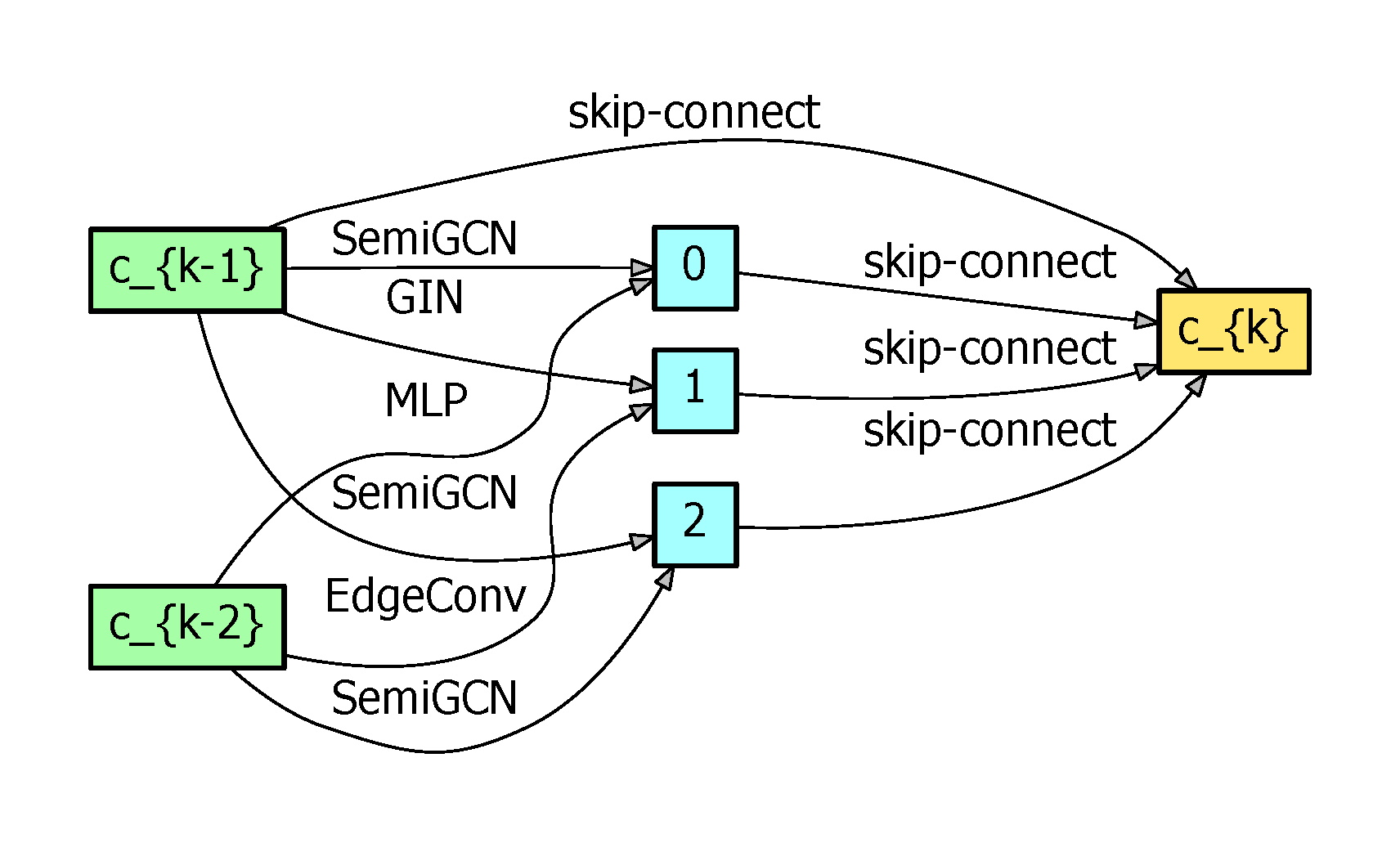
We show our search strategy in Figure 2. It is inspired by the method in DARTS [50]. Suppose that our GCN consist of M cells, and each cell consists of layers. Each layer is a latent representation. Each directed edge between two layers outputs a feature map at every forward propagation of neural network. The output of the layer is obtained by applying a reduction operation (e.g., concatenation) to all the intermediate nodes. The operation of each edge in the search space O is parameterized by architectural parameters , and is the architecture parameter of operation from the i-th layer to j-th layer . The output of i-th layer and one of inputs for j-th layer is given as:
where is some convolution operation in the search space O, and is the weight parameter of the graph convolution from the i-th layer to j-th layer. Each intermediate layer is based on the addition of all previous layers:
At the end of search, Equation (6) is replaced by: .
The trainable parameters are architecture parameters and the weight of cell or network w, and they are alternately trained. The loss function is denoted by which is a cross-entropy on validation set. When w is fixed, is updated by minimizing on the validation dataset, given as
When is fixed, w is updated by minimizing on the train dataset, given as
With the solutions of architecture parameters and the weight w, we can determine one cell for our ASGCN. Similar to other NAS implementations, our ASGCN is formed by stacking such cells together. Then we can fine-tune the whole network to optimize all the weights with the training set.
3.4. Comparison on Methods of Graph Partition
Besides our weight-based mini-batch for large-scale graph, we analyse three other ways of partition a graph. First, we consider dividing the large graph A into small non-overlapping graphs. Assuming that the number of nodes in each subgraph is q, the subgraphs are expressed as:
- (1)
- Fixed method: A common method is to use these subgraphs for training, and this is called fixed method.
- (2)
- Shuffle: Another method is shuffle. We can randomly select q nodes to constitute a subgraph for training in each epoch.
- (3)
- ClusterGCN [58]: In this method, a strategy called stochastic multiple partitions is proposed. It firstly utilizes the graph clustering algorithm METIS [56], to gather clusters. Then, in each epoch, it randomly samples () clusters and their between-cluster links to form a new batch to solve the unbalanced label distribution problem.
Obviously, for the Fixed method, it causes great data loss. As shown in the Figure 1, the white area of the adjacency matrix is the unused data. The amount of lost data is and the data utilization rate is . Assuming that can be divide by , then we have , and the data utilization rate is . The larger q is, the bigger data utilization rate is. means the whole graph is used for training. For the ClusterGCN method, the selection of number of nodes in a cluster is crucial. If the cluster is too large, it will cause a serious imbalance of sample distribution. As in the clustering process, data of the same category is naturally easy to be gathered together. As a result, the data of each batch are biased towards certain categories. If the cluster is too small, it is no different from the Shuffle method.
Different from ClusterGCN, we propose to select nodes according to a certain weight. We set the number of clusters as p for clustering, and each cluster has its own weight . When a cluster is selected too frequently, the weight will be reduced. The probability of being selected is also reduced. In this way, we can avoid serious imbalance of sample distribution and increase the diversity of training samples, which leads to a stable training process.
4. Experiments and Analysis
We evaluated our proposed method on real-world PolSAR data: Flevoland, and San Francisco datasets. The detail of them are below. The Flevoland dataset is an L-band four-look PolSAR data with a resolution of 1 × 6 m. It has a size of 750 × 1024 pixels and was acquired by NASA/JPL AIRSAR in 1989 from Netherlands. This dataset contains 15 terrains including: stem beans, rapeseed, bare soil, potatoes, beet, wheat, peas, wheat2, lucerne, barley, wheat3, grasses, forest, water, and buildings, which is widely used to evaluate the classification methods. The San Francisco dataset is the bay area with the golden gate bridge and its size is 1300 × 1300 pixels. It is C-band, single-look, and full-polarimetric SAR data acquired by RADARSAT-2 sensors, and includes five classes: water, vegetation, low-density urban, high-density urban, and the developed.
We conducted all the experiments on a computer with two 1080Ti GPUs (each with 11 GB memory). Our method was compared with five state-of-the-art algorithms consisting of two supervised methods: the SVM [24] and CNN [30], the unsupervised methods with pre-training: FS [22], W-DBN [23], and the semi-supervised methods: DSMR [46] and SemiGCN [9]. The coding was with PyTorch [59] and the GCN operators were implemented using Pytorch Geometric [60]. The initial random seed of the algorithm was fixed for fair comparison. We carried out each experiment for 20 times and reported both the average overall accuracy (OA) and standard deviation. In Flevoland and San Francisco datasets, the feature vectors were both with . Moreover, the Lee filtering [61] with 5 × 5 window size was applied to all the datasets for pre-processing to reduce the influence from the speckle noise of the PolSAR data. The parameters of algorithms are set as follows:
- SVM [24]: It was implemented with LibSVM (https://www.csie.ntu.edu.tw/~cjlin/libsvm/, accessed on 1 Apirl 2021). The kernel function was Radial Basis Function with and penalty coefficient for Flevoland dataset, and and penalty coefficient for San Francisco dataset.
- FS [22]: The number of super-pixels K was chosen among the interval [500, 3000], and the compactness of the super-pixels mpol is selected in the interval [20, 60].
- W-DBN [23]: W-DBN had two hidden layers, and node numbers were set to 50 and 100, respectively. The thresholds was chosen in the interval [0.95, 0.99]. The learning rate was set to 0.01. was set to 0, and the window size was set to 3 or 5.
- CNN [30]: The network included two convolution layers, two max-pooling layers and one fully connected layer. The sizes of the filters in two convolutional layers were 3 × 3 and 2 × 2, respectively, and the pooling size was 2 × 2. The momentum parameter was 0.9, and the weight decay rate was set to .
- DSMR [46]: The number of nearest neighbors and the regularization parameter were among the interval [10, 20] and [1 × , 1 × ], respectively. The weight decay rate is chosen in [, ].
- SemiGCN [9]: The number of hidden units was set to 32 or 64. The number of layers in the network was 3 or 4. Both normalization and self-connections were used. Learning rate and weight decay were set to and , respectively.
- ASGCN (ours): The coefficient of distance weighting was in the range [0, 1]. The number of subgraphs p was in the range [2000, 3000]. Learning rate and weight decay were and , respectively. The numbers of cells, and hidden units were discussed in the experiment.
4.1. Architecture and Parameter Discussion
In this subsection, we take the Flevoland dataset as an example to analyze the architecture and parameters.
(1) Weight-based Mini-batch Algorithm
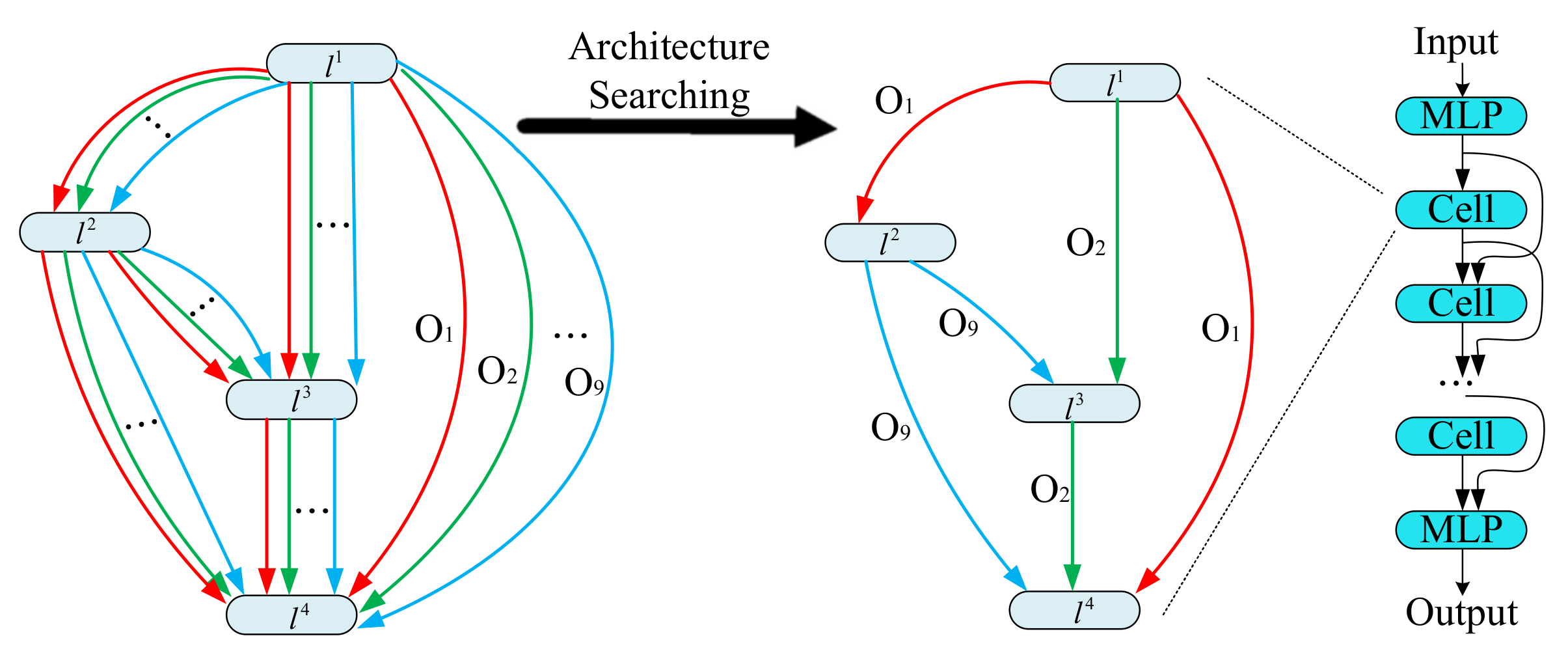
We verified our proposed strategy: weight-based mini-batch for graph partition and the results are shown in Figure 3. We used the searched architecture for comparison. The number of cells was 3, and the number of layers was 3. The graph was clustered into 2000 subgraphs. Other parameters were set as follows: The value of K in KNN algorithm: 32, batch size (16, 50, 300), learning rate: 0.001, weight decay: 0.0005, hidden units: 32, gradient clip: 5. We compared the convergence curves of test loss and OA values of four methods: ClusterGCN [58], Shuffle, Fixed, and the Weights (ours).
Experimental results indicated that our algorithm achieved better performance and more comprehensive data utilization than other methods. The convergence curve for the loss of our method was more stable than that of Shuffle and Fixed methods. Our method gained lower loss than that of the three other methods. Moreover, the OA of our weight-based method was the highest among theses three methods, since the weight assignment avoided imbalance of sample distribution and also resulted in a higher accuracy. The Shuffle method adopted random sampling each time, and the result was more unstable than that of other methods. The Fixed method utilized the same subgraphs, therefore its OA did not change in each epoch.
(2) Ablation Study on Architectures
In order to better understand the effects of the choices of hyper-parameters, we conducted ablation studies on the the number of cells and hidden units for the ASGCN.
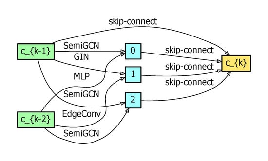
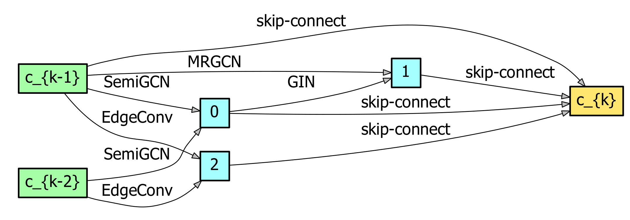
Firstly, fixing the parameters: the number of nearest neighbors and batch size were 30 and 400, respectively, we searched and showed the result of the top architecture in Figure 4. The name on each edge represented one of the operations from our search space. The edge without a name was a skip-connection. The inputs of each cell consisted of two previous cell outputs. The input of the first cell consisted of two identical graphs aggregated by MLP from original graph data. It can be seen that this cell included operations: gin, mr_conv, semi_gcn, and edge_conv.
Then we stacked the cells ranging from 2 to 4, and varied the number of units in 16, 32, 64, 128 for each architecture. The overall accuracies were obtained and listed in Table 1. It can be seen when the number of cells was 3 and the number of units is 32, the OA was the highest 99.31%, and the memory consumption was about 0.0568 MB. When the number of cells increased, the depth of the networks and the memory consumption also grew dramatically. However, the OA decreased. This indicated that the ASGCN could not be too deep which may result in over-fitting for this dataset, and three cells each with 32 units was a better choice for this dataset.
(3) Parameter Discussion
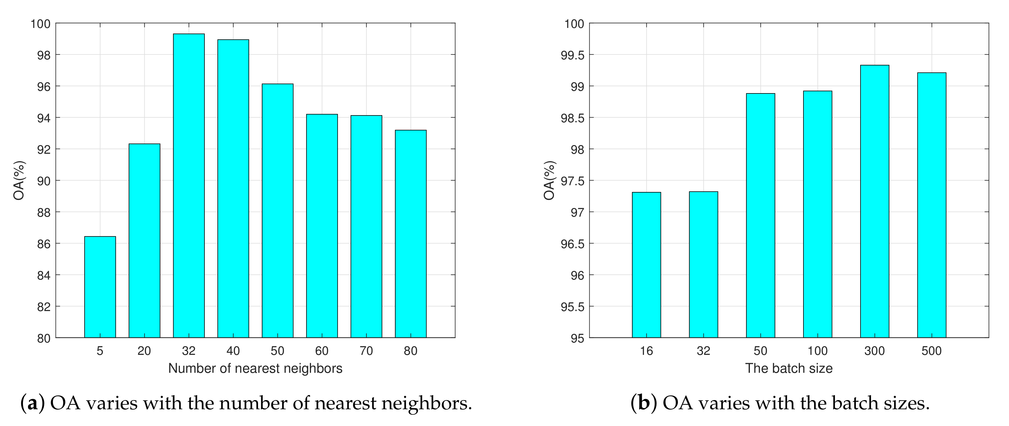
Moreover, we showed the influences of the number of nearest neighbors and the batch sizes on classification accuracy OA with the above architectures in Figure 5a,b, respectively. The influence caused by different numbers of nearest neighbors on the final results was great. It indicated that higher classification accuracy could be obtained when the number of nearest neighbors was near to 32. When it increased, OA could not be significantly improved, but it was not good if it was too small. For example, 5 and 20 adjacent neighbors may have caused loss of important connection information and led to the degradation of algorithm performance. It is worth noting that the time consumption of different number of nearest neighbors in the search and evaluation process had no significant difference, but the time cost in the phase of graph construction was much larger.
When the graph was divided into 2000 subgraphs, the performances with batch size 16 and 32 were poor. When the batch size exceeded 100, the classification accuracy of the algorithm became higher and started to remain stable. Small batch size resulted in incomplete information, thus the network could not process a large graph, and OA tended to float up and down.
4.2. Results on the Flevoland Dataset
For this dataset, the other parameters are as follows. The number of hidden units was set to 32. The number of cells and the number of layers were both 3. The dataset was divided into 2000 partitions, and batch size was 300. The number of nearest neighbors K was 32, and gradient clip was 5.
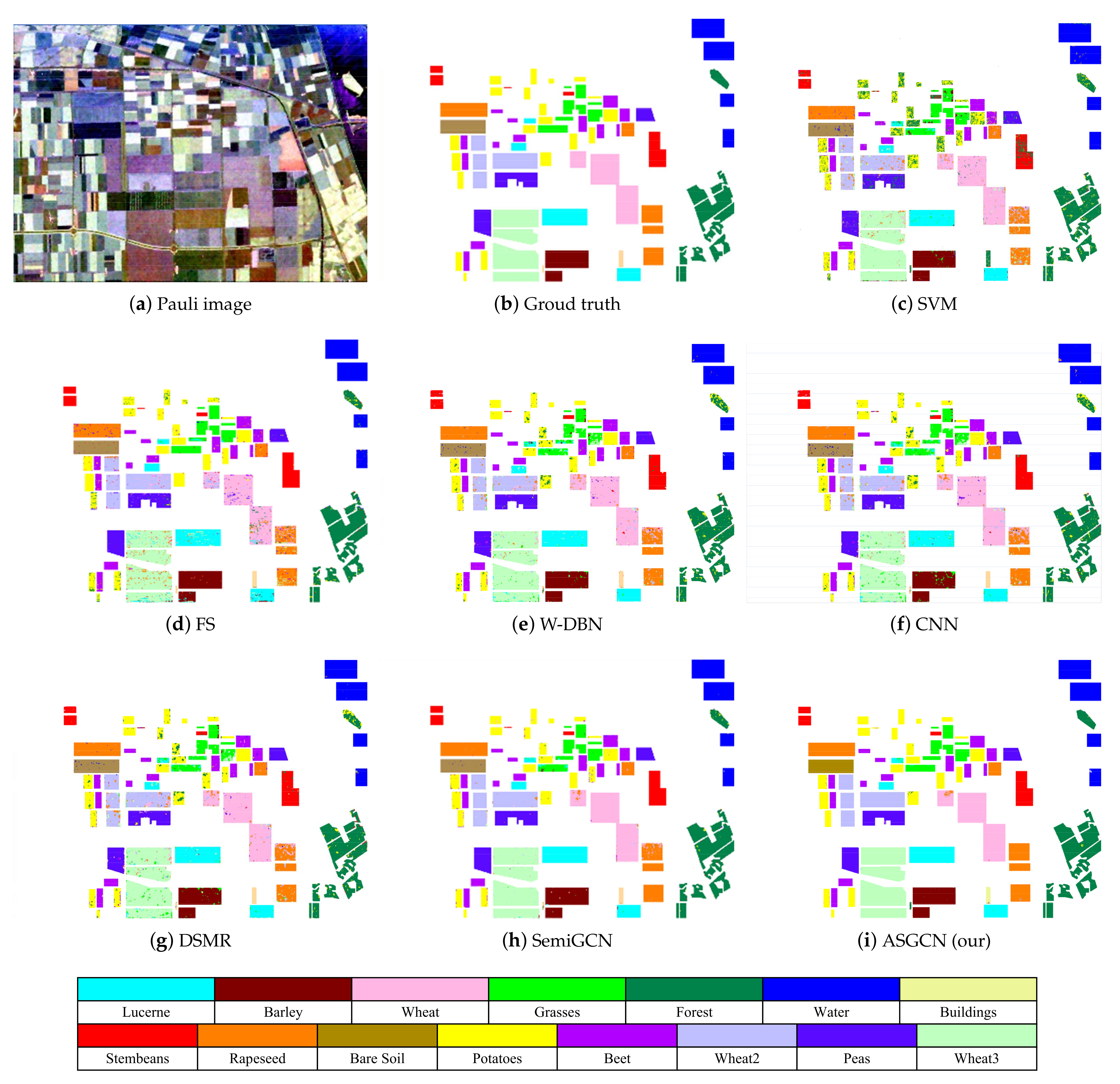
The classification maps are shown in Figure 6 and the accuracies are listed in Table 2. The mis-classified pixels of ASGCN were least and the OA was the highest at 99.31% among all the methods, and our method achieved high performance improvement in most categories, such as bare soil, wheat, peas, and water. It was 13.81% higher than that of the classical SVM in terms of OA. The performance of SVM was limited by the few labeled samples. Though CNN could take advantage of the labeled samples, it may have over-fitted with only 1% labeled samples for training, and yield an OA of 88.15%. The semi-supervised methods DSMR was inferior to that of the GCN based methods: SemiGCN and ASGCN, which is probably because the graph convolutional network could extract more differentiated features for classification. Moreover, since SemiGCN was constructed manually, its architecture may not have been optimal for this dataset, and its OA was lower than that of our ASGCN. By using the weight-based cluster method and differentiable neural architecture search applied to a reasonable search space, our algorithm effectively avoided over-fitting and unbalanced distribution of samples.It effectively improved the classification performance.
4.3. Results on the San Francisco Dataset
For this dataset, the number of hidden units was set to 24. The number of cells and the number of layers were both 3. The dataset was divided into 2000 partitions, and batch size was 300. The number of nearest neighbors K was 32, and gradient clip was 5.
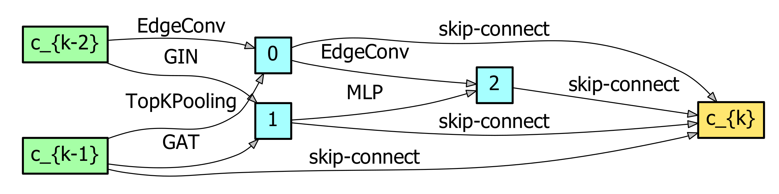
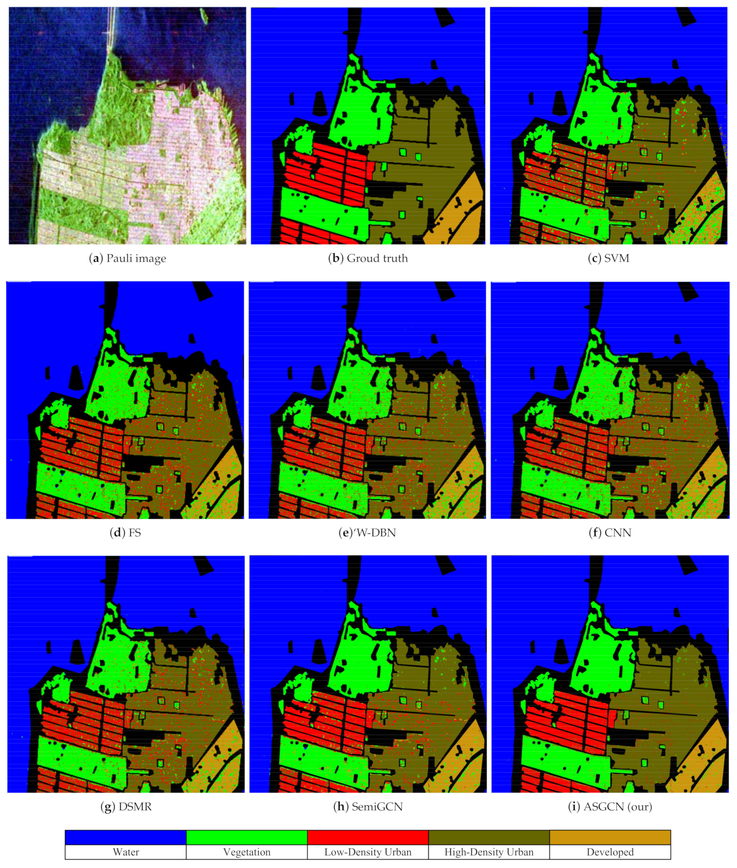
The searched architecture for this dataset is shown in Figure 7. Moreover, Figure 8 shows visual classification results, and Table 3 is the corresponding classification result of each category. The results showed that our ASGCN achieved the best accuracy at 96.80% among the studied algorithms. The semi-supervised methods: DSMR, SemiGCN and ASGCN, had greater improvement in classification performance compared with others as they can employed both the labeled and unlabeled samples to train the network. The classification accuracy of CNN was better than that of the SVM. However, CNN was a little inferior to that of the W-DBN. It is probably because only 1% labeled samples greatly weakened the fitting capability of the network. Compared with SemiGCN, our method attained higher OA. This is likely because its search space covered more possible situations and it could automatically search the most suitable network structure for the this dataset.
5. Conclusions
In this work, we propose a new neural network ASGCN based on architecture search for PolSAR image classification. The PolSAR data is represented by a fine grained graph, and a searching space is constructed for the automatical search of an optimal ASGCN. Our method avoids a great deal of work building networks manually. Addressing the memory cost caused by large scale graph, we proposed a weight-based mini-batch strategy, which greatly reduced the memory cost in a single epoch and maintained stable convergence. The experimental results on typical datasets, i.e., Flevoland and San Francisco, from different radar systems indicate that our method outperforms state-of-the-art methods for classification in the majority of the tested cases. The advantages of our ASGCN have been demonstrated by the experiments. That is, (1) Our ASGCN can avoid the conventionally manual design of the architecture which may result in tedious work in tuning the structure and hyper-parameters. (2) The proposed search space enables our model to find appropriate graph convolutional architecture for PolSAR classification. It may provide some inspirations for similar application. (3) The presented weight-based mini-batch strategy can decrease the memory cost and ensure training of large-scale dataset. However, similar to other NAS-based algorithm, our ASGCN costs more time for search of an optimal architecture than the training of other semi-supervised algorithms, such as the DSMR [46], and SemiGCN [9]. Anyway, our ASGCN enhances the classification accuracy compared with some of the state-of-the-art methods. This may provide inspirations for the construction of new GCN and other automatic design of networks for PolSAR classification. In the future, more techniques will be studied to speed up the search process of our ASGCN. Moreover, we will investigate other graph clustering approaches in [62,63] to improve our weighted mini-batch strategy.
Author Contributions
Conceptualization and methodology, H.L., F.S. and T.Z.; writing, D.X., Y.L., R.Y. and J.L. All authors have read and agreed to the published version of the manuscript.
Funding
This research was funded by the National Natural Science Foundation of China (Nos. 61976164, 61876220, 61876221, 61836009 and U1701267), the Project supported the Foundation for Innovative Research Groups of the National Natural Science Foundation of China (No. 61621005), the Program for Cheung Kong Scholars and Innovative Research Team in University (No. IRT_15R53), the Fund for Foreign Scholars in University Research and Teaching Programs (the 111 Project) (No. B07048), the Science Foundation of Xidian University (Nos. 10251180018 and 10251180019), the National Science Basic Research Plan in Shaanxi Province of China (Nos. 2020JM-194 and 2019JQ-657), and the Key Special Project of China High Resolution Earth Observation System-Young Scholar Innovation Fund.
Acknowledgments
We thank the reviewers for their valuable comments.
Conflicts of Interest
The authors declare no conflict of interest.
References
- Lee, J.S.; Ainsworth, T.L. An overview of recent advances in polarimetric SAR information extraction: Algorithms and applications. In Proceedings of the IEEE International Geoscience and Remote Sensing Symposium, Honolulu, HI, USA, 25–30 July 2010; pp. 851–854. [Google Scholar]
- Cloude, S.R.; Pottier, E. An entropy based classification scheme for land applications of polarimetric SAR. IEEE Trans. Geosci. Remote Sens. 1997, 35, 68–78. [Google Scholar] [CrossRef]
- Lee, J.S.; Pottier, E. Polarimetric Radar Imaging: From Basics to Applications; CRC Press: Boca Raton, FL, USA, 2009. [Google Scholar]
- Zhang, Z.; Wang, H.; Xu, F.; Jin, Y.Q. Complex-valued convolutional neural network and its application in polarimetric SAR image classification. IEEE Trans. Geosci. Remote Sens. 2017, 55, 7177–7188. [Google Scholar] [CrossRef]
- McNairn, H.; Brisco, B. The application of C-band polarimetric SAR for agriculture: A review. Can. J. Remote Sens. 2004, 30, 525–542. [Google Scholar] [CrossRef]
- Freeman, A. Fitting a two-component scattering model to polarimetric SAR data from forests. IEEE Trans. Geosci. Remote Sens. 2007, 45, 2583–2592. [Google Scholar] [CrossRef]
- Ulaby, F.T.; Elachi, C. Radar Polarimetry for Geoscience Applications; Artech House, Inc.: Norwood, MA, USA, 1990. [Google Scholar]
- Zhou, J.; Cui, G.; Zhang, Z.; Yang, C.; Liu, Z.; Wang, L.; Li, C.; Sun, M. Graph Neural Networks: A Review of Methods and Applications. arXiv 2018, arXiv:1812.08434. [Google Scholar]
- Kipf, T.N.; Welling, M. Semi-supervised classification with graph convolutional networks. In Proceedings of the 5th International Conference on Learning Representations, Toulon, France, 24–26 April 2017. [Google Scholar]
- Zoph, B.; Le, Q.V. Neural Architecture Search with Reinforcement Learning. In Proceedings of the 5th International Conference on Learning Representations, Toulon, France, 24–26 April 2017. [Google Scholar]
- Lee, J.S.; Grunes, M.R.; Ainsworth, T.L.; Du, L.J.; Schuler, D.L.; Cloude, S.R. Unsupervised classification using polarimetric decomposition and the complex Wishart classifier. IEEE Trans. Geosci. Remote Sens. 1999, 37, 2249–2258. [Google Scholar]
- Lee, J.S.; Grunes, M.R.; Pottier, E.; Ferro-Famil, L. Unsupervised terrain classification preserving polarimetric scattering characteristics. IEEE Trans. Geosci. Remote Sens. 2004, 42, 722–731. [Google Scholar]
- Freeman, A.; Durden, S.L. A three-component scattering model for polarimetric SAR data. IEEE Trans. Geosci. Remote Sens. 1998, 36, 963–973. [Google Scholar] [CrossRef] [Green Version]
- Silva, W.B.; Freitas, C.C.; Sant’Anna, S.J.; Frery, A.C. Classification of segments in PolSAR imagery by minimum stochastic distances between Wishart distributions. IEEE J. Sel. Top. Appl. Earth Obs. Remote Sens. 2013, 6, 1263–1273. [Google Scholar] [CrossRef] [Green Version]
- Du, L.; Lee, J. Fuzzy classification of earth terrain covers using complex polarimetric SAR data. Int. J. Remote Sens. 1996, 17, 809–826. [Google Scholar] [CrossRef]
- Kersten, P.R.; Lee, J.S.; Ainsworth, T.L. Unsupervised classification of polarimetric synthetic aperture radar images using fuzzy clustering and EM clustering. IEEE Trans. Geosci. Remote Sens. 2005, 43, 519–527. [Google Scholar] [CrossRef]
- Vasile, G.; Ovarlez, J.P.; Pascal, F.; Tison, C. Coherency Matrix Estimation of Heterogeneous Clutter in High-Resolution Polarimetric SAR Images. IEEE Geosci. Remote Sens. Lett. 2010, 48, 1809–1826. [Google Scholar] [CrossRef]
- Pallotta, L.; Clemente, C.; De Maio, A.; Soraghan, J.J. Detecting Covariance Symmetries in Polarimetric SAR Images. IEEE Geosci. Remote Sens. Lett. 2017, 55, 80–95. [Google Scholar] [CrossRef]
- Pallotta, L.; Maio, A.D.; Orlando, D. A Robust Framework for Covariance Classification in Heterogeneous Polarimetric SAR Images and Its Application to L-Band Data. IEEE Geosci. Remote Sens. Lett. 2019, 57, 104–119. [Google Scholar] [CrossRef]
- Pallotta, L.; Orlando, D. Polarimetric covariance eigenvalues classification in SAR images. IEEE Geosci. Remote Sens. Lett. 2018, 16, 746–750. [Google Scholar] [CrossRef]
- Eltoft, T.; Doulgeris, A.P. Model-Based Polarimetric Decomposition With Higher Order Statistics. IEEE Geosci. Remote Sens. Lett. 2019, 16, 992–996. [Google Scholar] [CrossRef] [Green Version]
- Guo, Y.; Jiao, L.; Wang, S.; Wang, S.; Liu, F.; Hua, W. Fuzzy superpixels for polarimetric SAR images classification. IEEE Trans. Fuzzy Syst. 2018, 26, 2846–2860. [Google Scholar] [CrossRef]
- Liu, F.; Jiao, L.; Hou, B.; Yang, S. POL-SAR Image Classification Based on Wishart DBN and Local Spatial Information. IEEE Trans. Geosci. Remote Sens. 2016, 54, 1–17. [Google Scholar] [CrossRef]
- Fukuda, S.; Hirosawa, H. Polarimetric SAR image classification using support vector machines. IEICE Trans. Electron. 2001, 84, 1939–1945. [Google Scholar]
- Lardeux, C.; Frison, P.L.; Tison, C.; Souyris, J.C.; Stoll, B.; Fruneau, B.; Rudant, J.P. Support vector machine for multifrequency SAR polarimetric data classification. IEEE Trans. Geosci. Remote Sens. 2009, 47, 4143–4152. [Google Scholar] [CrossRef]
- She, X.; Yang, J.; Zhang, W. The boosting algorithm with application to polarimetric SAR image classification. In Proceedings of the 1st Asian and Pacific Conference on Synthetic Aperture Radar, Huangshan, China, 5–9 November 2007; pp. 779–783. [Google Scholar]
- Zou, T.; Yang, W.; Dai, D.; Sun, H. Polarimetric SAR image classification using multifeatures combination and extremely randomized clustering forests. EURASIP J. Adv. Signal Proc. 2009, 2010, 1–9. [Google Scholar] [CrossRef] [Green Version]
- He, C.; Li, S.; Liao, Z.; Liao, M. Texture classification of PolSAR data based on sparse coding of wavelet polarization textons. IEEE Trans. Geosci. Remote Sens. 2013, 51, 4576–4590. [Google Scholar] [CrossRef]
- Salehi, M.; Sahebi, M.R.; Maghsoudi, Y. Improving the accuracy of urban land cover classification using Radarsat-2 PolSAR data. IEEE J. Sel. Top. Appl. Earth Obs. Remote Sens. 2013, 7, 1394–1401. [Google Scholar]
- Zhou, Y.; Wang, H.; Xu, F.; Jin, Y.Q. Polarimetric SAR image classification using deep convolutional neural networks. IEEE Geosci. Remote Sens. Lett. 2016, 13, 1935–1939. [Google Scholar] [CrossRef]
- Mohammadimanesh, F.; Salehi, B.; Mahdianpari, M.; Gill, E.; Molinier, M. A new fully convolutional neural network for semantic segmentation of polarimetric SAR imagery in complex land cover ecosystem. ISPRS J. Photo. Remote Sens. 2019, 155, 223–236. [Google Scholar] [CrossRef]
- Bi, H.; Xu, F.; Wei, Z.; Xue, Y.; Xu, Z. An active deep learning approach for minimally supervised PolSAR image classification. IEEE Trans. Geosci. Remote Sens. 2019, 57, 9378–9395. [Google Scholar] [CrossRef]
- Hänsch, R.; Hellwich, O. Semi-supervised learning for classification of polarimetric SAR-data. In Proceedings of the IEEE International Geoscience and Remote Sensing Symposium, Cape Town, South Africa, 12–17 July 2009; Volume 3, pp. 987–990. [Google Scholar]
- Uhlmann, S.; Kiranyaz, S.; Gabbouj, M. Semi-supervised learning for ill-posed polarimetric SAR classification. Remote Sens. 2014, 6, 4801–4830. [Google Scholar] [CrossRef] [Green Version]
- Niu, X.; Ban, Y. An adaptive contextual SEM algorithm for urban land cover mapping using multitemporal high-resolution polarimetric SAR data. IEEE J. Sel. Top. Appl. Earth Obs. Remote Sens. 2012, 5, 1129–1139. [Google Scholar] [CrossRef]
- Zhu, X.J. Semi-Supervised Learning Literature Survey; University of Wisconsin-Madison: Madison, WI, USA, 2005. [Google Scholar]
- Subramanya, A.; Talukdar, P.P. Graph-based semi-supervised learning. Synth. Lect. Artif. Intell. Mach. Learn. 2014, 8, 1–125. [Google Scholar] [CrossRef] [Green Version]
- Liu, W.; He, J.; Chang, S.F. Large graph construction for scalable semi-supervised learning. In Proceedings of the 27th International Conference on Machine Learning (ICML 2010), Haifa, Israel, 21–24 June 2010. [Google Scholar]
- Liu, H.; Wang, Y.; Yang, S.; Wang, S.; Feng, J.; Jiao, L. Large polarimetric SAR data semi-supervised classification with spatial-anchor graph. IEEE J. Sel. Top. Appl. Earth Obs. Remote Sens. 2016, 9, 1439–1458. [Google Scholar] [CrossRef]
- Liu, H.; Zhu, D.; Yang, S.; Hou, B.; Gou, S.; Xiong, T.; Jiao, L. Semisupervised feature extraction with neighborhood constraints for polarimetric SAR classification. IEEE J. Sel. Top. Appl. Earth Obs. Remote Sens. 2016, 9, 3001–3015. [Google Scholar] [CrossRef]
- Liu, H.; Yang, S.; Gou, S.; Zhu, D.; Wang, R.; Jiao, L. Polarimetric SAR feature extraction with neighborhood preservation-based deep learning. IEEE J. Sel. Top. Appl. Earth Obs. Remote Sens. 2016, 10, 1456–1466. [Google Scholar] [CrossRef]
- Liu, H.; Yang, S.; Gou, S.; Chen, P.; Wang, Y.; Jiao, L. Fast classification for large polarimetric SAR data based on refined spatial-anchor graph. IEEE Geosci. Remote Sens. Lett. 2017, 14, 1589–1593. [Google Scholar] [CrossRef]
- Liu, H.; Yang, S.; Gou, S.; Liu, S.; Jiao, L. Terrain Classification based on Spatial Multi-attribute Graph using Polarimetric SAR Data. Appl. Soft Comput. 2018, 68, 24–38. [Google Scholar] [CrossRef]
- Liu, H.; Wang, Z.; Shang, F.; Yang, S.; Gou, S.; Jiao, L. Semi-supervised tensorial locally linear embedding for feature extraction using PolSAR data. IEEE J. Sel. Top. Signal Proc. 2018, 12, 1476–1490. [Google Scholar] [CrossRef]
- Liu, H.; Wang, F.; Yang, S.; Hou, B.; Jiao, L.; Yang, R. Fast Semisupervised Classification Using Histogram-Based Density Estimation for Large-Scale Polarimetric SAR Data. IEEE Geosci. Remote Sens. Lett. 2019, 16, 1844–1848. [Google Scholar] [CrossRef]
- Liu, H.; Shang, F.; Yang, S.; Gong, M.; Zhu, T.; Jiao, L. Sparse Manifold-Regularized Neural Networks for Polarimetric SAR Terrain Classification. IEEE Trans. Neural Netw. Learn. Syst. 2019, 31, 3007–3016. [Google Scholar] [CrossRef]
- Bi, H.; Sun, J.; Xu, Z. A graph-based semisupervised deep learning model for PolSAR image classification. IEEE Geosci. Remote Sens. Lett. 2018, 57, 2116–2132. [Google Scholar] [CrossRef]
- Yao, Q.; Wang, M.; Chen, Y.; Dai, W.; Yi-Qi, H.; Yu-Feng, L.; Wei-Wei, T.; Qiang, Y.; Yang, Y. Taking human out of learning applications: A survey on automated machine learning. arXiv 2018, arXiv:1810.13306. [Google Scholar]
- Elsken, T.; Metzen, J.H.; Hutter, F. Neural architecture search: A survey. J. Mach. Learn. Res. 2019, 20, 1–21. [Google Scholar]
- Liu, H.; Simonyan, K.; Yang, Y. DARTS: Differentiable Architecture Search. In Proceedings of the 7th International Conference on Learning Representations, New Orleans, LA, USA, 6–9 May 2019. [Google Scholar]
- Li, G.; Xiong, C.; Thabet, A.; Ghanem, B. DeeperGCN: All You Need to Train Deeper GCNs. arXiv 2020, arXiv:2006.07739. [Google Scholar]
- Wang, Y.; Sun, Y.; Liu, Z.; Sarma, S.E.; Bronstein, M.M.; Solomon, J.M. Dynamic Graph CNN for Learning on Point Clouds. ACM Trans. Graph. 2019, 38. [Google Scholar] [CrossRef] [Green Version]
- Veličković, P.; Cucurull, G.; Casanova, A.; Romero, A.; Liò, P.; Bengio, Y. Graph Attention Networks. In Proceedings of the International Conference on Learning Representations, Vancouver, BC, Canada, 30 April–3 May 2018. [Google Scholar]
- Xu, K.; Hu, W.; Leskovec, J.; Jegelka, S. How Powerful are Graph Neural Networks? In Proceedings of the International Conference on Learning Representations, New Orleans, LA, USA, 6–9 May 2019. [Google Scholar]
- Gao, H.; Ji, S. Graph U-Nets. In Proceedings of the 36th International Conference on Machine Learning, Long Beach, CA, USA, 9–15 June 2019; pp. 2083–2092. [Google Scholar]
- Karypis, G.; Kumar, V. A fast and high quality multilevel scheme for partitioning irregular graphs. SIAM J. Sci. Comput. 1998, 20, 359–392. [Google Scholar] [CrossRef]
- Dwivedi, V.P.; Joshi, C.K.; Laurent, T.; Bengio, Y.; Bresson, X. Benchmarking Graph Neural Networks. arXiv 2020, arXiv:2003.00982. [Google Scholar]
- Chiang, W.; Liu, X.; Si, S.; Li, Y.; Bengio, S.; Hsieh, C. Cluster-GCN: An Efficient Algorithm for Training Deep and Large Graph Convolutional Networks. In Proceedings of the 25th ACM SIGKDD International Conference on Knowledge Discovery & Data Mining, KDD 2019, Anchorage, AK, USA, 4–8 August 2019; pp. 257–266. [Google Scholar] [CrossRef] [Green Version]
- Paszke, A.; Gross, S.; Chintala, S.; Chanan, G.; Yang, E.; DeVito, Z.; Lin, Z.; Desmaison, A.; Antiga, L.; Lerer, A. Automatic differentiation in PyTorch. In Proceedings of the 31st Conference on Neural Information Processing Systems (NIPS 2017), Long Beach, CA, USA, 4–9 December 2017. [Google Scholar]
- Fey, M.; Lenssen, J.E. Fast Graph Representation Learning with PyTorch Geometric. In Proceedings of the ICLR Workshop on Representation Learning on Graphs and Manifolds, New Orleans, LA, USA, 6–9 May 2019. [Google Scholar]
- Lee, J.S.; Grunes, M.R.; De Grandi, G. Polarimetric SAR speckle filtering and its implication for classification. IEEE Trans. Geosci. Remote Sens. 1999, 37, 2363–2373. [Google Scholar]
- Fortunato, S. Community detection in graphs. Phys. Rep. 2010, 486, 75–174. [Google Scholar] [CrossRef] [Green Version]
- Fortunato, S.; Hric, D. Community detection in networks: A user guide. Phys. Rep. 2016, 659, 1–44. [Google Scholar] [CrossRef] [Green Version]
Figure 1.
Our weight-based graph partition strategy. Left: The whole graph A are partitioned into p parts: , which are represented by the black blocks using a graph clustering algorithm. Right: We sample q black blocks according to the weights to form a batch, which is in colored block.
Figure 1.
Our weight-based graph partition strategy. Left: The whole graph A are partitioned into p parts: , which are represented by the black blocks using a graph clustering algorithm. Right: We sample q black blocks according to the weights to form a batch, which is in colored block.

Figure 2.
The architecture searching for our architecture search method based graph convolutional network (ASGCN). In this example, there is one cell which includes four layers: , , , . The connection between layers are searched from the operation space O, which contains nine operations: , , …, .
Figure 2.
The architecture searching for our architecture search method based graph convolutional network (ASGCN). In this example, there is one cell which includes four layers: , , , . The connection between layers are searched from the operation space O, which contains nine operations: , , …, .

Figure 3.
The test loss and overall accuracy (OA) of our weight-based mini-batch strategy (i.e., Weights) compared with other methods: ClusterGCN [58], Fixed and Shuffle.
Figure 3.
The test loss and overall accuracy (OA) of our weight-based mini-batch strategy (i.e., Weights) compared with other methods: ClusterGCN [58], Fixed and Shuffle.

Figure 4.
The searched result of our ASGCN method, which stacks three cells, each including three layers on the Flevoland dataset. Here, , and c_{k-1}, c_{k-2}, and c_{k} are feature maps for each cell.
Figure 4.
The searched result of our ASGCN method, which stacks three cells, each including three layers on the Flevoland dataset. Here, , and c_{k-1}, c_{k-2}, and c_{k} are feature maps for each cell.

Figure 5.
Classification accuracy versus the number of nearest neighbors and the batch sizes on the Flevoland dataset. The batch size is fixed to 300 in (a), and the number of nearest neighbors is fixed to 32 in (b). Other parameter settings in (a) and (b) are the same as described in Section 4.1(1).

Figure 6.
Classification results of different methods on the Flevoland dataset. (a) Pauli RGB image. (b) Ground truth, (c) support vector machines (SVM) [24], (d) fuzzy super-pixel (FS) [22], (e) Wishart Deep Belief Network (W-DBN) [23], (f) convolutional neural network (CNN) [30], (g) sparse manifold regularization (DSMR) [46], (h) semi-graph convolutional network (SemiGCN) [9], and (i) ASGCN (ours).

Figure 7.
The searched result of our ASGCN method, which stacks three cells, each including three layers on the San Francisco dataset. Here, and c_{k-1}, c_{k-2}, and c_{k} are feature maps for each cell.
Figure 7.
The searched result of our ASGCN method, which stacks three cells, each including three layers on the San Francisco dataset. Here, and c_{k-1}, c_{k-2}, and c_{k} are feature maps for each cell.

Figure 8.
Classification results of different methods on the San Francisco dataset. (a) Pauli RGB image, (b) Ground truth, (c) SVM [24], (d) FS [22], (e) W-DBN [23], (f) CNN [30], (g) DSMR [46], (h) SemiGCN [9], and (i) ASGCN (ours).


Table 1.
The OA and memory consumption vary with the number of cells and hidden units for our ASGCN method on the Flevoland dataset.
Table 1.
The OA and memory consumption vary with the number of cells and hidden units for our ASGCN method on the Flevoland dataset.
| Number of Cells | Hidden Units | Params. (MB) | Test OA (%) |
|---|---|---|---|
| 2 | 16 | 0.0115 | 94.31 |
| 2 | 32 | 0.0388 | 97.21 |
| 2 | 64 | 0.1412 | 95.51 |
| 2 | 128 | 0.5362 | 95.98 |
| 3 | 16 | 0.0161 | 95.19 |
| 3 | 32 | 0.0568 | 99.31 |
| 3 | 64 | 0.2118 | 99.01 |
| 3 | 128 | 0.8168 | 98.37 |
| 4 | 16 | 0.0207 | 94.77 |
| 4 | 32 | 0.0747 | 98.96 |
| 4 | 64 | 0.2825 | 98.65 |
| 4 | 128 | 1.0974 | 97.47 |
Table 2.
The classification accuracy of all methods with 1% training samples on the Flevoland dataset.
Table 2.
The classification accuracy of all methods with 1% training samples on the Flevoland dataset.
| Methods | SVM [24] | FS [22] | W-DBN [23] | CNN [30] | DSMR [46] | SemiGCN [9] | ASGCN (Ours) |
|---|---|---|---|---|---|---|---|
| Stembeans | 83.22 ± 1.893 | 85.13 ± 1.952 | 90.73 ± 2.331 | 93.33 ± 2.132 | 99.82 ± 1.568 | 97.67 ± 1.512 | 97.77 ± 1.231 |
| Rapeseed | 89.01 ± 1.251 | 79.23 ± 1.614 | 90.57 ± 2.451 | 97.45 ± 2.270 | 90.28 ± 1.412 | 97.73 ± 1.486 | 94.71 ± 1.529 |
| Bare Soil | 88.16 ± 1.810 | 76.39 ± 1.642 | 91.71 ± 2.953 | 97.73 ± 2.245 | 86.67 ± 1.356 | 97.29 ± 1.302 | 99.23 ± 0.831 |
| Potatoes | 95.28 ± 1.833 | 83.18 ± 1.846 | 85.67 ± 2.851 | 91.27 ± 2.315 | 99.79 ± 1.632 | 92.78 ± 1.230 | 99.34 ± 0.911 |
| Beet | 86.35 ± 1.917 | 95.23 ± 1.832 | 99.86 ± 2.135 | 99.69 ± 2.412 | 99.76 ± 1.237 | 95.54 ± 1.759 | 98.91 ± 0.938 |
| Wheat2 | 84.47 ± 1.905 | 76.35 ± 1.512 | 89.34 ± 2.412 | 84.91 ± 2.561 | 86.21 ± 1.242 | 94.62 ± 1.637 | 98.74 ± 1.579 |
| Peas | 87.56 ± 1.258 | 85.31 ± 1.831 | 92.81 ± 2.137 | 85.09 ± 2.418 | 98.47 ± 1.122 | 94.06 ± 1.448 | 98.94 ± 0.422 |
| Wheat3 | 76.73 ± 2.018 | 85.11 ± 1.677 | 89.92 ± 2.168 | 99.79 ± 2.111 | 95.56 ± 1.193 | 99.59 ± 1.649 | 99.22 ± 1.144 |
| Lucerne | 87.18 ± 1.316 | 85.81 ± 1.525 | 89.05 ± 2.144 | 70.23 ± 2.104 | 83.84 ± 1.258 | 86.73 ± 1.857 | 96.70 ± 1.700 |
| Barley | 82.26 ± 1.643 | 86.18 ± 1.984 | 88.73 ± 2.587 | 33.73 ± 2.139 | 98.36 ± 1.269 | 97.89 ± 1.268 | 99.34 ± 0.621 |
| Wheat | 81.38 ± 1.700 | 85.12 ± 1.713 | 90.52 ± 2.584 | 95.21 ± 2.516 | 92.03 ± 1.144 | 92.57 ± 1.372 | 98.93 ± 1.137 |
| Grasses | 94.88 ± 1.676 | 82.56 ± 1.656 | 89.43 ± 2.691 | 45.32 ± 2.547 | 64.51 ± 1.581 | 86.75 ± 1.592 | 99.08 ± 1.356 |
| Forest | 81.09 ± 1.748 | 91.63 ± 1.872 | 89.22 ± 2.687 | 99.87 ± 2.138 | 98.50 ± 1.343 | 99.11 ± 1.337 | 98.93 ± 1.483 |
| Water | 83.59 ± 1.420 | 79.20 ± 1.757 | 91.19 ± 2.783 | 88.26 ± 2.147 | 83.16 ± 1.214 | 98.93 ± 1.441 | 99.98 ± 0.473 |
| Buildings | 80.73 ± 1.627 | 76.16 ± 1.729 | 90.73 ± 2.553 | 87.42 ± 2.159 | 99.73 ± 1.231 | 96.43 ± 1.022 | 92.58 ± 1.650 |
| OA | 85.50 ± 1.907 | 84.02 ± 1.738 | 90.33 ± 2.486 | 88.15 ± 2.279 | 92.31 ± 1.311 | 95.55 ± 1.036 | 99.31 ± 1.732 |
Table 3.
Classification accuracy of all methods with 1% training samples on the San Francisco dataset.
Table 3.
Classification accuracy of all methods with 1% training samples on the San Francisco dataset.
| Methods | Water | Vegetation | Low-Density Urban | High-Density Urban | Developed | OA |
|---|---|---|---|---|---|---|
| SVM [24] | 98.69 ± 1.988 | 84.45 ± 1.486 | 50.74 ± 1.364 | 73.53 ± 1.659 | 60.92 ± 1.422 | 85.39 ± 1.907 |
| FS [22] | 90.63 ± 1.776 | 79.77 ± 1.675 | 61.33 ± 1.987 | 80.13 ± 1.888 | 68.21 ± 1.811 | 83.25 ± 1.803 |
| W-DBN [23] | 99.77 ± 2.780 | 89.56 ± 2.913 | 57.64 ± 2.761 | 83.72 ± 2.661 | 65.21 ± 2.703 | 89.75 ± 2.770 |
| CNN [30] | 98.56 ± 2.257 | 81.71 ± 2.164 | 53.24 ± 2.538 | 85.03 ± 2.252 | 62.35 ± 2.290 | 87.73 ± 2.267 |
| DSMR [46] | 99.89 ± 1.464 | 91.63 ± 1.634 | 69.34 ± 1.656 | 87.78 ± 1.552 | 74.91 ± 1.589 | 92.40 ± 1.529 |
| SemiGCN [9] | 98.93 ± 1.469 | 92.03 ± 1.730 | 92.23 ± 1.489 | 91.21 ± 1.349 | 91.09 ± 1.147 | 94.57 ± 1.469 |
| ASGCN (ours) | 99.87 ± 0.881 | 93.77 ± 1.258 | 93.64 ± 1.109 | 93.92 ± 1.529 | 82.33 ± 1.178 | 96.80 ± 1.393 |
Publisher’s Note: MDPI stays neutral with regard to jurisdictional claims in published maps and institutional affiliations. |
© 2021 by the authors. Licensee MDPI, Basel, Switzerland. This article is an open access article distributed under the terms and conditions of the Creative Commons Attribution (CC BY) license (https://creativecommons.org/licenses/by/4.0/).
Share and Cite
MDPI and ACS Style
Liu, H.; Xu, D.; Zhu, T.; Shang, F.; Liu, Y.; Lu, J.; Yang, R. Graph Convolutional Networks by Architecture Search for PolSAR Image Classification. Remote Sens. 2021, 13, 1404. https://0-doi-org.brum.beds.ac.uk/10.3390/rs13071404
AMA Style
Liu H, Xu D, Zhu T, Shang F, Liu Y, Lu J, Yang R. Graph Convolutional Networks by Architecture Search for PolSAR Image Classification. Remote Sensing. 2021; 13(7):1404. https://0-doi-org.brum.beds.ac.uk/10.3390/rs13071404
Chicago/Turabian StyleLiu, Hongying, Derong Xu, Tianwen Zhu, Fanhua Shang, Yuanyuan Liu, Jianhua Lu, and Ri Yang. 2021. "Graph Convolutional Networks by Architecture Search for PolSAR Image Classification" Remote Sensing 13, no. 7: 1404. https://0-doi-org.brum.beds.ac.uk/10.3390/rs13071404
Note that from the first issue of 2016, this journal uses article numbers instead of page numbers. See further details here.