Article

Mangrove and Saltmarsh Distribution Mapping and Land Cover Change Assessment for South-Eastern Australia from 1991 to 2015

1
School of Life & Environmental Sciences, Faculty of Science, Engineering and Built Environment, Deakin University, Warrnambool, VIC 3280, Australia
2
School of Life & Environmental Sciences, Faculty of Science, Engineering and Built Environment, Deakin University, Burwood, VIC 3125, Australia
*
Author to whom correspondence should be addressed.
Submission received: 22 February 2021 / Revised: 31 March 2021 / Accepted: 4 April 2021 / Published: 8 April 2021
(This article belongs to the Special Issue Remote Sensing of Wetland Vegetation Patterns and Dynamics)

Abstract

:
Coastal wetland ecosystems, such as saltmarsh and mangroves, provide a wide range of important ecological and socio-economic services. A good understanding of the spatial and temporal distribution of these ecosystems is critical to maximising the benefits from restoration and conservation projects. We mapped mangrove and saltmarsh ecosystem transitions from 1991 to 2015 in south-eastern Australia, using remotely sensed Landsat data and a Random Forest classification. Our classification results were improved by the addition of two physical variables (Shuttle Radar Topographic Mission (SRTM), and Distance to Water). We also provide evidence that the addition of post-classification, spatial and temporal, filters improve overall accuracy of coastal wetlands detection by up to 16%. Mangrove and saltmarsh maps produced in this study had an overall User Accuracy of 0.82–0.95 and 0.81–0.87 and an overall Producer Accuracy of 0.71–0.88 and 0.24–0.87 for mangrove and saltmarsh, respectively. We found that mangrove ecosystems in south-eastern Australia have lost an area of 1148 ha (7.6%), whilst saltmarsh experienced an overall increase in coverage of 4157 ha (20.3%) over this 24-year period. The maps developed in this study allow local managers to quantify persistence, gains, and losses of coastal wetlands in south-eastern Australia.

Graphical Abstract

1. Introduction

Coastal wetland ecosystems (mangrove, saltmarsh, and seagrasses) provide a wide range of important ecological and socio-economic services to coastal areas [1], including provisioning, coastal protection, recreational and aesthetic uses, and climate change mitigation through soil formation and carbon sequestration [2,3,4,5]. However, the extent of coastal wetlands has significantly decreased worldwide as a result of anthropogenic impacts, particularly near populated areas [6,7]. Coastal wetland ecosystems are susceptible to a range of natural and anthropogenic-related threats, including climate change, and the associated impacts of sea level rise, storms, tidal surges, and changes in precipitation and temperature [8,9,10], coastal development, and conversion to agriculture, such as stock grazing [11].
In Australia, mangroves and saltmarshes occur throughout coastal regions, covering an area of approximately 25,000 km2 [12,13]. Although they are protected under the Environment Protection and Biodiversity Conservation Act 1999 [14], they have seen extensive loss since European colonisation. Large losses of coastal wetland ecosystems have been documented over the past 50 years due to increasing agriculture and urbanisation near estuarine fringes [15] or climate change-associated extreme weather events [8]. In temperate regions of south-eastern Australia, around 20 percent of Australia’s mangroves and saltmarshes have been lost since colonisation [16], with some estuaries losing up to 80 percent [15]. As a consequence, coastal wetland ecosystems have been a focus of many conservation and restoration projects in temperate and sub-tropical regions of Australia [17,18,19]. The success of such projects requires a good understanding of spatial and temporal ecosystem distribution to inform better management strategies and to ensure effort is directed towards appropriate areas [20,21,22].
Comprehensive, statewide mapping and inventory studies of coastal wetlands have been completed over the past two decades along the south-eastern coast of Australia, using a mixture of airborne and on-ground surveys (Victoria [23] and New South Wales [19,24]). Although some historical mapping has been undertaken with the use of aerial photography [19,25] and archival maps [23] in specific study areas, the majority of these statewide maps were made for single years. This is a result of the methodologies used to obtain these maps (aerial and on-ground surveys), which are expensive and not widely available, often prohibiting the collection of frequent repeat surveys [26,27]. As a result, there is a lack of temporally consistent data at an appropriate temporal and spatial resolution for ecosystem monitoring and management.
Remotely sensed satellite data provide a fast, cost-effective, and efficient method to monitor the distribution of coastal wetlands ecosystems [27,28,29,30]. The Landsat satellites (Thematic Mapper, TM; Enhanced TM+, ETM+; and Operational Land Imager, OLI) have been the most widely used sensors for mapping coastal wetlands distribution [28,31,32,33,34], as they provide access to a high temporal frequency (every 16 days), medium resolution (~30 m), long-term dataset over the past 35+ years [35]. This long temporal coverage allows investigation of transitional patterns of ecosystems and land uses across broad spatial scales [36,37,38,39]. While multiple mangrove maps have been developed at global scales [31,33], consistent and repeatable time-series are lacking, particularly those trained for local use mapping and application.
Recent development of machine learning (ML) methods provides new opportunities for accurately mapping coastal wetlands ecosystems [34]. Traditionally, coastal wetland mapping using satellite data has been performed using individual vegetation indices [34]. Numerous classical vegetation indices (i.e., Normalised Difference Vegetation Index, Enhanced Vegetation Index, and Normalised Difference Water Index) and novel vegetation indices (i.e., Combined Mangrove Recognition Index and Modular Mangrove Recognition Index) have been tested for coastal wetlands detection [40,41]. These indices are generally good at differentiating flooded vegetated areas from adjacent water sources or non-flooded vegetation [40]. However, they often struggle to differentiate between specific flooded vegetated types, such as mangroves, saltmarshes, and freshwater wetlands [42]. On the other hand, machine learning algorithms such as random forest, artificial neural networks, or support vector regression have proven to be more successful in mapping coastal wetlands distribution than single indices [40,42,43]. These models generally use a list of individual multispectral bands and vegetation indices [40,44]. However, although important for forest detection [45,46], physical variables such as Shuttle Radar Topographic Mission (SRTM) elevation and Distance to Water (DistW) have rarely been used for the detection of coastal wetlands [42]. As their name indicates, coastal wetlands are known for occurring across the land-sea interface [47]. Therefore, we hypothesised that the addition of a DistW layer would improve coastal wetland detection with satellite data. Additionally, these ecosystems have very low growth rates in south-eastern Australia due to the colder climate [48], and therefore will benefit from the use of SRTM elevation as a variable, despite it being collected for a single year (2000; [49]).
In this study, we present triennial mangrove and saltmarsh distribution maps at 30 m resolution from 1991 to 2015 across the south-eastern coast of Australia. We use a combination of cloud-based (Google Earth Engine) and local computing to map coastal areas by applying a Random Forest (RF) model to Landsat time series data. We also propose the use of two physical variables (SRTM and Distance to Water) and a set of post-classification filters to improve mangrove and saltmarsh modelling. Finally, we perform a land-use change analysis to assess the gains and losses of mangrove and saltmarsh extent over the 24-year period. The map outputs from this study provide a long-term time series of the dynamics of these important coastal ecosystems, which can help with management by quantifying ecosystem losses or gains and persistence, along with impacts on their associated ecosystem services.

2. Materials and Methods
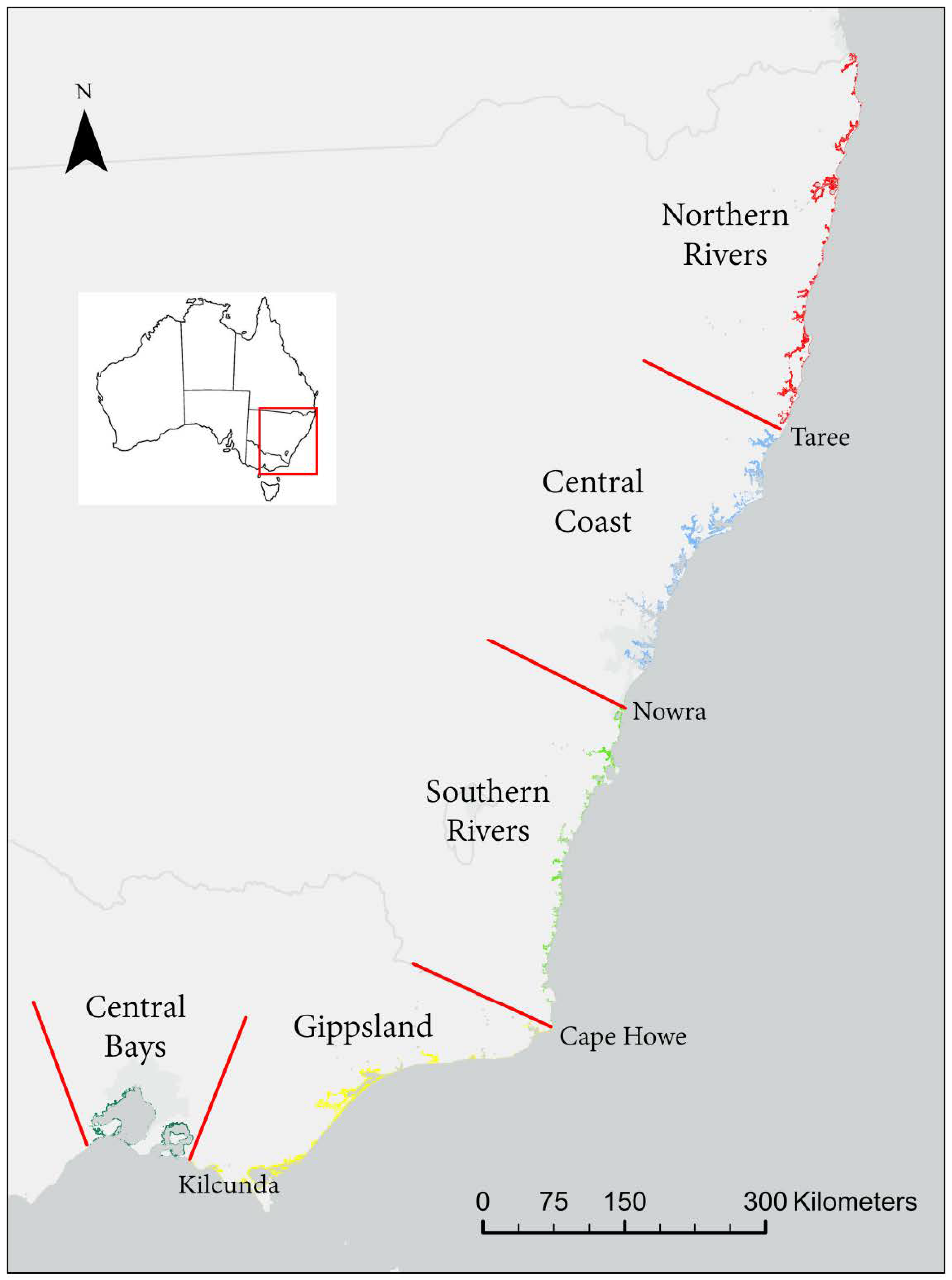
2.1. Study Area

We focused our research on the south-eastern coast of Australia (Figure 1), which comprises two climatic regions: temperate in Victoria (VIC) and sub-tropical in New South Wales (NSW). The southernmost distribution of mangrove ecosystems in the world can be found in Corner Inlet (VIC). Air temperatures in this region can reach 0 °C during winter, making mangrove survival very difficult [48]. Only one species of mangrove has adapted to live in these conditions (Avicennia marina), forming dwarf stands with a height range between 1 and 3.5 m [50] and covering an area of approximately 5000 ha in VIC [23]. In contrast, saltmarshes along the VIC coast encompass a variety of species with different structural forms such as woody shrubs (e.g., Tecticornia arbuscula and Salicornia quinqueflora) and grasses (e.g., Distichlis disichophylla and Austrostipa stipoides), and cover an area of approximately 20,000 ha [23].
Mangrove forests in the sub-tropical regions of NSW are more diverse, both in species composition (with up to 4 species: Avicennia marina, Aegiceras corniculatum, Bruguiera gymnorhiza, and Excoecaria agallocha) and height range (between 2 and 17 m), and cover an area of approximately 12,000 ha [19]. Saltmarsh can be found in estuaries along the entire NSW coastline, covering an estimated total area of over 7200 ha [19]. Saltmarsh species diversity decreases as latitude increases along the coast of NSW, with Jervis Bay (Nowra, Figure 1) being the northern limit for several species [51]. On the Northern Rivers region of NSW (Figure 1), saltmarshes are dominated by a few plant species very similar to tall graminoids or pastureland, such as Saltwater Couch (Sporobolus virginicus), Samphire (Sarcocornia quinqueflora), and rushes, including Sea Rush (Juncus kraussii).

2.2. Landsat Imagery Acquisition and Pre-Processing

We obtained all datasets and their sub-products from the GEE platform repository. We used atmospherically corrected surface reflectance (SR) data from the Landsat 5 TM and Landsat 8 OLI/TIRS sensors, which include Level-1 Precision Terrain (L1TP) processed data [52,53]. These datasets include a pixel Quality Assessment (QA) band generated from the CFMASK algorithm, which populates cloud, cloud shadow, and snow/ice pixels, as well as a per-pixel saturation mask [54].
We used SR data to produce annual cloud-free composites, ranging from the 1 January to the 31 December, for the years 1988, 1991, 1994, 1997, 1999, 2003, 2006, 2009, 2013, 2015, and 2018, at approximately at 3-year intervals; note that the years 2000 and 2012 have been changed for the years 1999 and 2013, respectively. This is due to lack of suitable Landsat 5 SR data for our area of interest while Landsat 7 was working correctly (2000–2002), as well as lack of data due to Landsat 5 TM sensor failure in November 2011, one year before the launch of Landsat 8 in 2013. We based the choice of triennial (every 3 years) maps as a trade-off between local memory and computing capabilities and the minimum gap to detect coastal wetland changes. Landsat 5 TM data were used for the maps from 1988 to 2009, while Landsat 8 OLI was used for 2013, 2015 and 2018.
We used the cloud/shadow removal script within GEE to remove pixels that might be affected by artifacts or cloud contamination [55]. For this, we used a combination of: (1) the quality assessment (QA) band by discarding pixels labelled as cloud or cloud shadows by the CFMASK algorithm [54]; and (2) the GEE median reducer by picking the median pixel value in each band over the annual composites to further remove cloud-contaminated pixels that might not have been discarded by the QA.

2.3. Data Masking

Data masking has been widely used for improving the overall accuracy of coastal wetlands distribution maps by reducing processing time and decreasing the vegetation diversity of coastal areas [32,40,56]. In this study, four consecutive masks were applied to the annual cloud-free composites before classification:
First, we masked all areas on the Landsat images that were higher than 20 m using SRTM data within GEE [49]. We determined 20 m to be the maximum height for mangrove and saltmarsh forests in south-eastern Australia using ground-truthed data from Navarro, et al. [57].
Second, we applied a RF classifier using training classes from the Department of Planning, Industry and Environment of NSW from the year 2007 [58] and the Department of Environment, Land, Water, and Planning of VIC [59], to create a water layer and sand layer for each individual timestep, which were subsequently masked from the Landsat images.
Third, we eliminated water bodies whose distance to the 3 closest water bodies was on average greater than 250 m apart (i.e., small ponds and water reservoirs) from the previously generated water layer, as vegetation associated with these water bodies could potentially be mistaken as coastal wetlands. Coastal wetlands ecosystems in temperate and sub-tropical regions of Australia do not generally form wide forests, but grow in relatively thin strips around estuaries and embayments due to the colder climate [48] and other anthropogenic pressures [23]. Therefore, a Distance to Water (DistW) layer was created with the remaining water layer and all pixels that had a DistW over 1000 m were masked from the Landsat images.
Finally, preliminary analyses of the data revealed that foredune vegetation has the potential to be falsely classified as coastal wetlands (especially saltmarsh). Consequently, a Distance to Sand (DistS) layer was created and all pixels whose distance to water was greater than distance to sand were again masked from the Landsat images. This mask allowed us to remove coastal vegetated areas that were not in direct contact with water and therefore helped us avoid false classifications of foredune vegetation as coastal wetlands.

2.4. Coastal Wetlands Classification

2.4.1. Training and Validation Datasets

Due to its length and biogeographical characteristics, the south-eastern coast of Australia was split into five sub-regions (Figure 1): three in NSW (Northern Rivers, from Tweed Head to Manning River at Taree; Central Coast, from Manning River to Shoalhaven River at Nowra; and Southern Rivers, from Shoalhaven River to Cape Howe) and two in VIC (Gippsland, from Cape Howe to Powlett River at Kilcunda; and Central Bays, which include Westernport and Port Phillip Bay). We used ancillary data collected from various sources to create training and validation datasets for the 5 classes used in this study (Mangrove, Saltmarsh, Built, Crop, and Other Vegetation). Mangrove and Saltmarsh training datasets were obtained for each region from existing wetland maps derived from airborne photogrammetry for NSW [19] and VIC [23]. The other 3 classes (Built, Crop, and Other Vegetation) were derived from land use maps from 2006 obtained from the Department of Planning, Industry, and Environment for NSW [58] and the Department of Environment, Land, Water, and Planning for VIC [59].
Having set the refined training region, all classes were statistically filtered (with the 90th percentile function) and visually inspected to remove inadequate training samples. Of the remaining sample dataset, a proportional number of samples (5%) were randomly selected for every class (Mangrove, Saltmarsh, Built, Crop, and Other Vegetation), per region for the year 2006 (closest one to the years all data was obtained). Proportional stratified sampling and statistical filtering are necessary to address imbalanced class problems, allowing the removal of outliers from the sample bag [60]. All samples were then separated into training (70%, n = 107,150) and validation datasets (30%, n = 45,938).
Due to the spectral differences between Landsat 5 and Landsat 8 imagery [61], the training regions were revised using high resolution imagery from Google Earth for the year 2013 (first Landsat 8 annual composite), and a new set of training and validation datasets were created. A full dissection of all training and validation datasets for every class and every sub-region can be found in the supplementary (Table S1).

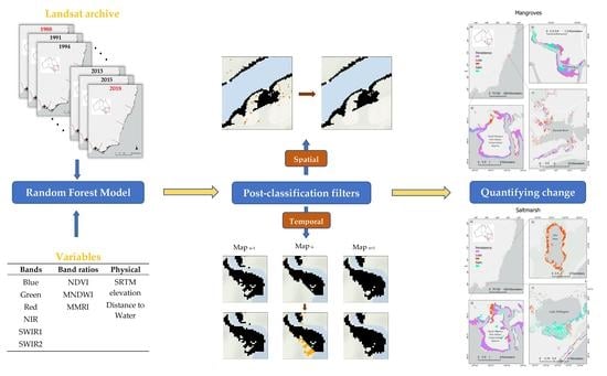
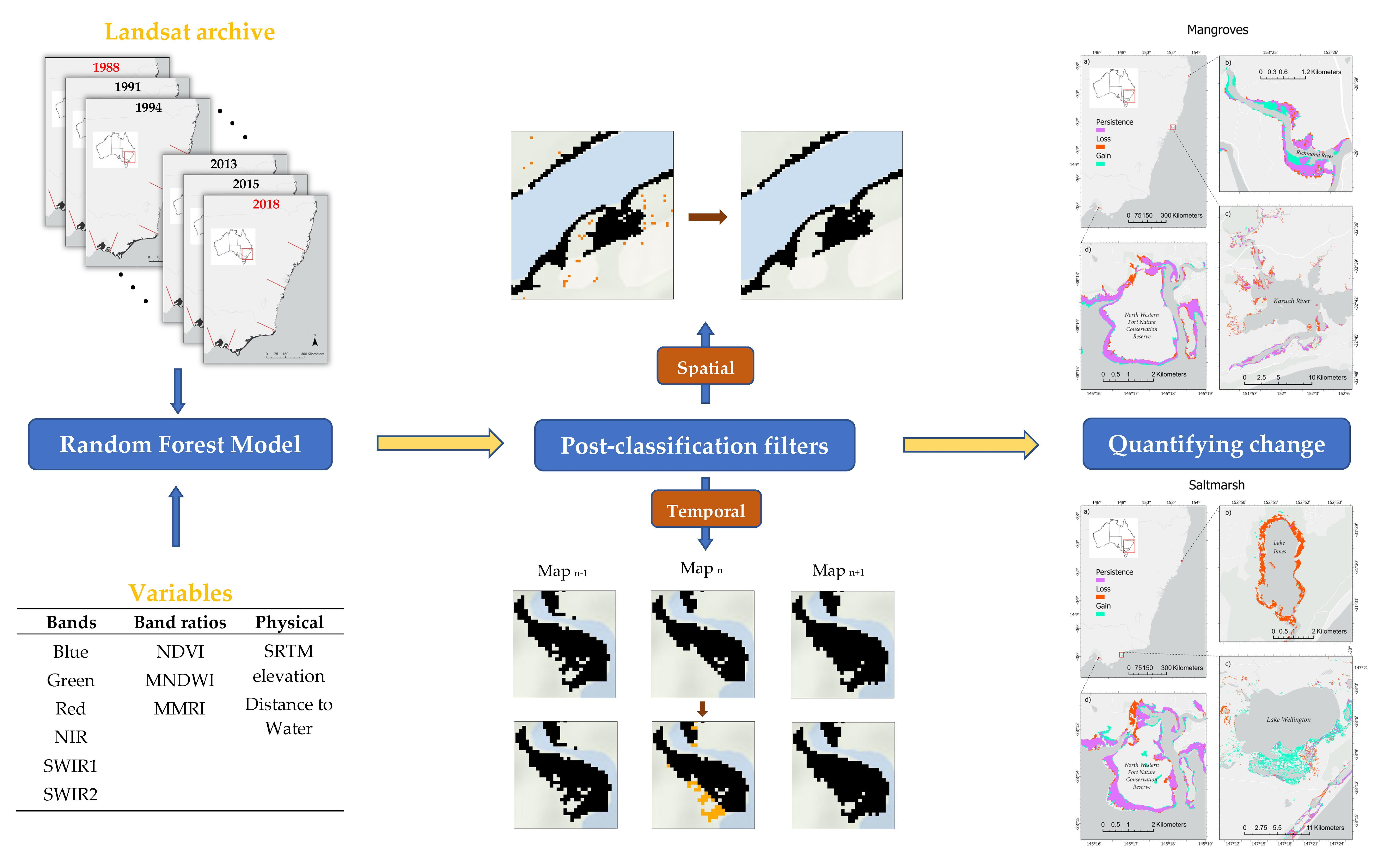
2.4.2. Random Forest Model

Finally, we performed two RF classifications [62] at every sub-region (one for the Landsat 5 annual composite of the year 2006, and the other for the Landsat 8 annual composite of the year 2013) to categorise the south-eastern coast of Australia into 5 distinct classes: Mangrove, Saltmarsh, Built, Cropland, and Other Vegetation. To obtain the full range of the Landsat imagery, the two models were applied respectively to the remaining annual composites (2006/Landsat 5 for 1988–2009 and 2013/Landsat 8 for 2015–2018)
RF classification [62] has been widely applied for coastal land-use modelling [40,42,43]. RF works by aggregating the predictions made by multiple uncorrelated decision trees (ntree). Each tree is trained on a randomly selected with replacement subset of the training samples (roughly 2/3), while the remaining third are used for estimating the Out-of-bag (OOB) error. At each node of the trees, a number of predictors (mtry) are selected at random from all the variables to split the nodes. In our case, both the ntree and mtry were left as default (500 and square root of the total number of all predictors, respectively).
The RF models were implemented using the randomForest package in R [63] using a combination of spectral bands and indices and physical variables. The variables used within the model are defined in Table 1. To test the individual performance of the physical variables (SRTM height and Distance to Water, hereafter DistW), we created 4 RF models with different combinations of variables: (1) Spectral; (2) Spectral + DistW; (3) Spectral + SRTM; and (4) Spectral + DistW + SRTM.

2.4.3. Post-Classification Filters

Two different post-classification filters were applied to the resulting maps: a spatial and a temporal filter.
First, due to the pixel-based nature of the classification method, a post-classification spatial filter was applied. Mangrove and saltmarsh pixels that share at least one side with neighbouring pixels of the same ID were grouped into clumps. Then, we used two constraints to remove mangrove and saltmarsh clumps that are very uncommon (less than 5% of all pixels in the ground-truthed training datasets met these criteria), which are summarised in Table 2. First, it is very uncommon for any mangrove or saltmarsh patch to be less than 0.2 ha and 0.5 ha in size respectively, so we excluded smaller patches for these classes; and second, it is very uncommon for any mangrove or saltmarsh patch to be more than 45 m (1 pixel) and 120 m (4 pixels) from water, respectively. However, we cannot eliminate all of these patches as the ones that are actually farther from that distance are usually the bigger ones (more than 1 ha in size for mangroves and 5 ha for saltmarsh). Therefore, we used a second constraint eliminating all mangrove patches that are more than 45 m away from a water body and less than 5 ha in size; and all saltmarsh patches that are more than 120 m away from water and less than 5 ha in size. This post-classification filter assisted in eliminating noise in the classification in the form of small and isolated mangrove and saltmarsh clusters likely to be artefacts. Two consecutive focal functions using a moving 3*3 window and a modal function (most repeated surrounding category) were then applied to fill the holes left by the spatial filter.
Second, a temporal filter was used to identify transitions between classes that are implausible. The temporal filter examines every pixel of three consecutive maps and, if the central map is found to be different than the edges, then it is reclassified to match its temporal neighbour class, as shown in Table 3. Similar temporal filters have been applied for mangrove change analysis by Diniz et al. [40].

2.4.4. Accuracy Assessment and Validation

We created confusion matrices using the independent validation datasets to test the Overall Accuracy (OA), Kappa statistics and class-specific balanced accuracies (using the R package “caret” [67]) of the 4 models we created [68]: (1) Spectral; (2) Spectral + DistW; (3) Spectral + SRTM; and (4) Spectral + DistW + SRTM.
We then proceeded to evaluate the performance of the most accurate model (as determined by the previous statistics) at 3 different stages (after classification, after spatial filter, after temporal filter). We used the confusion matrices to determine the Producer Accuracy (PA) and User Accuracy (UA) of the distribution of mangroves and saltmarsh. This allowed us to test and compare the benefits of each of the post-classification filters used in this study for improving coastal wetlands detection.

2.5. Land-Cover Transitions

We compared the extent of area classified as mangrove or saltmarsh within each of the 5 regions between 1991 and 2015 (1988 and 2018 were discarded due to not being able to apply the temporal filter to them). In addition, we assessed annual change intensity in terms of gains (gross annual gain divided by the size of the category at the final time point of the interval) and losses (gross annual loss divided by the size of the category at the initial time point of the interval) for all the land cover classes using the R package “intensity.analysis” [69]. We then compared these intensities with uniform change in the study area to distinguish whether transitions between land cover classes were random (relatively dormant) or systematic (active; Pontius et al. [70]). Finally, we evaluated transitional patterns (gains and losses in hectares from the earliest distribution maps to the latest) between our two ecosystems of interest and all the other classes (i.e., Built, Croplands, Mangroves, Other Vegetation, Saltmarsh, Water, and Sand).

3. Results

3.1. Random Forest Classification

A consistent time-series of ten annual land-cover maps was created for the south-eastern coast of Australia for the period 1991–2015 at approximately three-year time intervals. We used the independent validation datasets to create confusion matrices specific for every sub-region and for the whole area of interest (Table S2). Based on the OA, Kappa statistics and class-specific balanced accuracies (summarised in Table 4 for the 2006/Landsat 5 model), the best RF model was model (4), which included spectral bands (blue, green, red, NIR, SWIR1, and SWIR2), spectral indices (NDVI, MNDWI, and MMRI) and the two physical indices (SRTM and DistW). The average overall accuracy of this model across all regions of interest is 89% for the Landsat 5 TM model (Table 4) and 88% for the Landsat 8 OLI model. For simplicity, and due to its similarity with the 2006/Landsat 5 model, the results for the 2013/Landsat 8 model are shown in Table S3. On average, the addition of SRTM and DistW to the RF model improved the OA and Kappa statistics by approximately 2% (Table 4 and Table S3). However, the two classes of interest of our study (mangroves and saltmarsh) improved by up to 4% and 10%, respectively. The triennial land-cover maps created using this RF model are freely available for download as tif files from https://0-doi-org.brum.beds.ac.uk/10.6084/m9.figshare.14343500 (accessed on 7 April 2021).

3.2. Post-Classification Filters

The performance of the two post-classification filters (2006/Landsat 5 and 2013/Landsat 8) in terms of Producer and User Accuracy can be found in Table 5 and Table S4, respectively. We used the independent validation datasets (using 30% of our samples, Table S1) to create a confusion matrix (Table S2) from which the Producer and User Accuracy were derived. We compared the accuracy of our models at three different stages (after initial classification, after spatial filter and after temporal filter). We observe improvements in User Accuracy of up to 17% in some cases after applying the post-classification filters (Table 5 and Table S4). However, Producer Accuracy tends to slightly decrease due to the inherent nature of the spatial post-classification filter (removal of mangrove and saltmarsh pixels, some of which are rightly classified from the beginning), being as low as 0.24 for saltmarsh in Northern Rivers (Table 5 and Table S4). In general, User and Producer Accuracy is substantially higher for mangroves than for saltmarsh across both regions, and is also higher in VIC than it is in NSW for both ecosystems (Table 5 and Table S4).

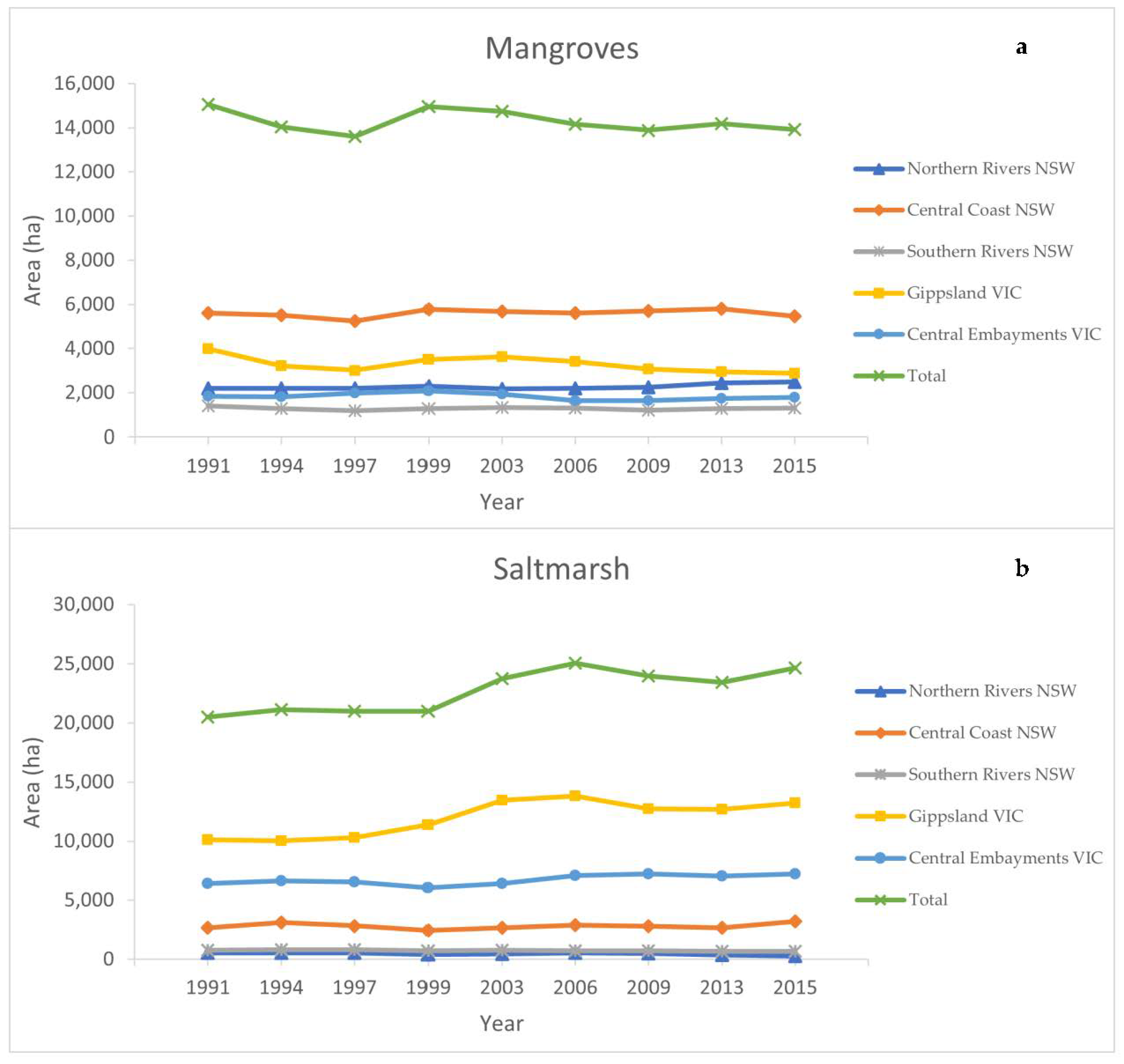
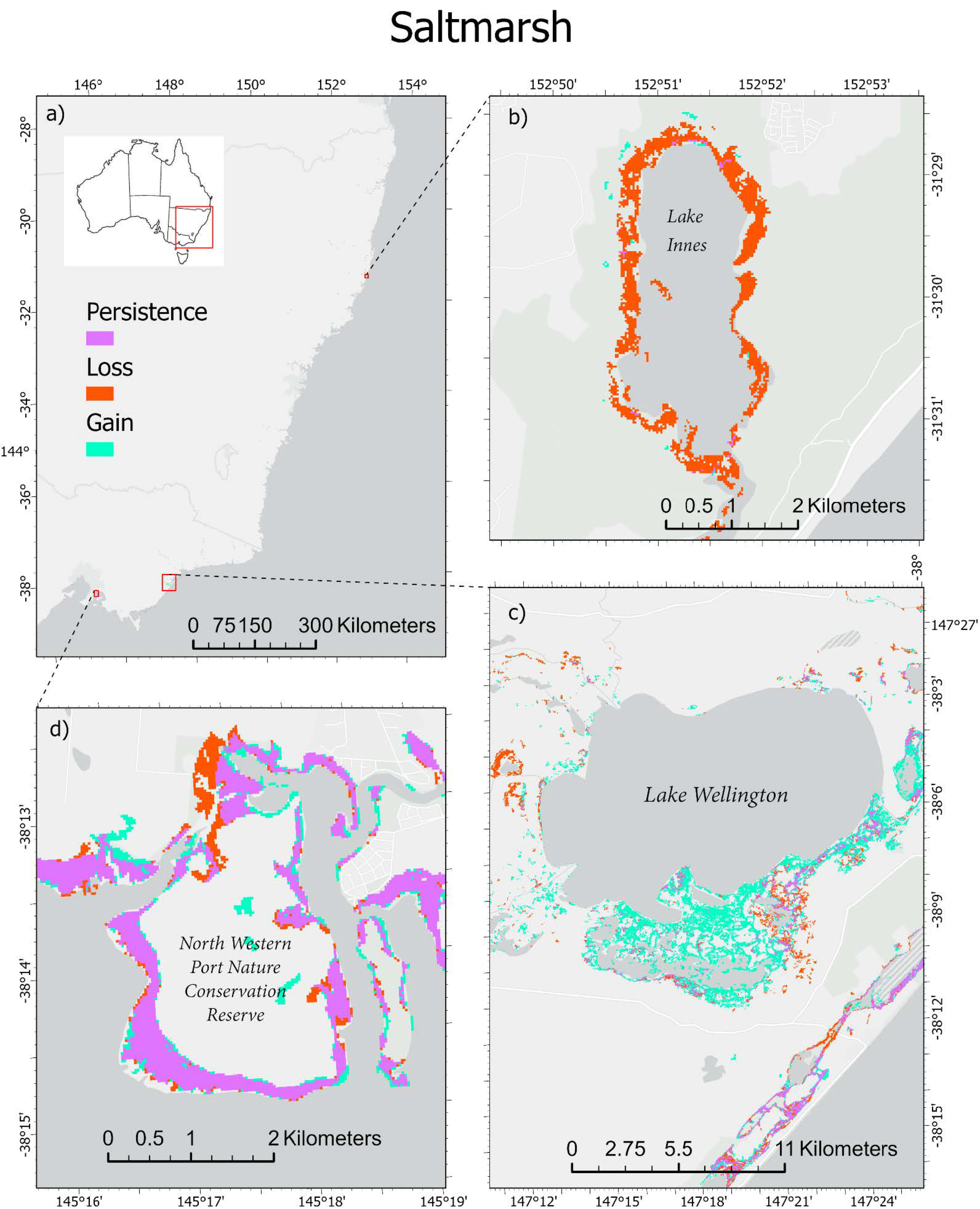
3.3. Coastal Wetlands in South-Eastern Australia

Overall, there was a decrease in mangrove coverage (−1148 ha or 7.6%), with two periods of slight but constant decrease (1991–1997 and 1999–2006) and a period of relatively rapid increase (1997–1999). Mangrove area remained fairly stable around 14,000 ha after 2006 (Figure 2). On the other hand, saltmarsh experienced an overall increase in coverage (+4157 ha or 20.3%), most of which happened between 1999 and 2006, remaining stable before and after that period (Figure 2).
The gains, losses, and persistence between 1991 and 2015 of our two classes of interest (mangroves and saltmarsh) across the whole region can be visualised in Figure 3 and Figure 4, respectively, along with several noteworthy zoomed-in examples. Figure 3b and Figure 4b show mangrove extension and saltmarsh loss to water, respectively. Figure 3c shows an example of extensive mangrove declines in Karuah River (Central Coast, NSW), while Figure 4c shows extensive saltmarsh expansion (associated with the rapid saltmarsh increase between 1999 and 2006) in Lake Wellington (Gippsland, VIC). Finally, Figure 3d and Figure 4d show the same area of the northern shore of WesternPort (Central Bays, VIC), where mangroves have lost area to saltmarsh ecosystems while gaining area through water.

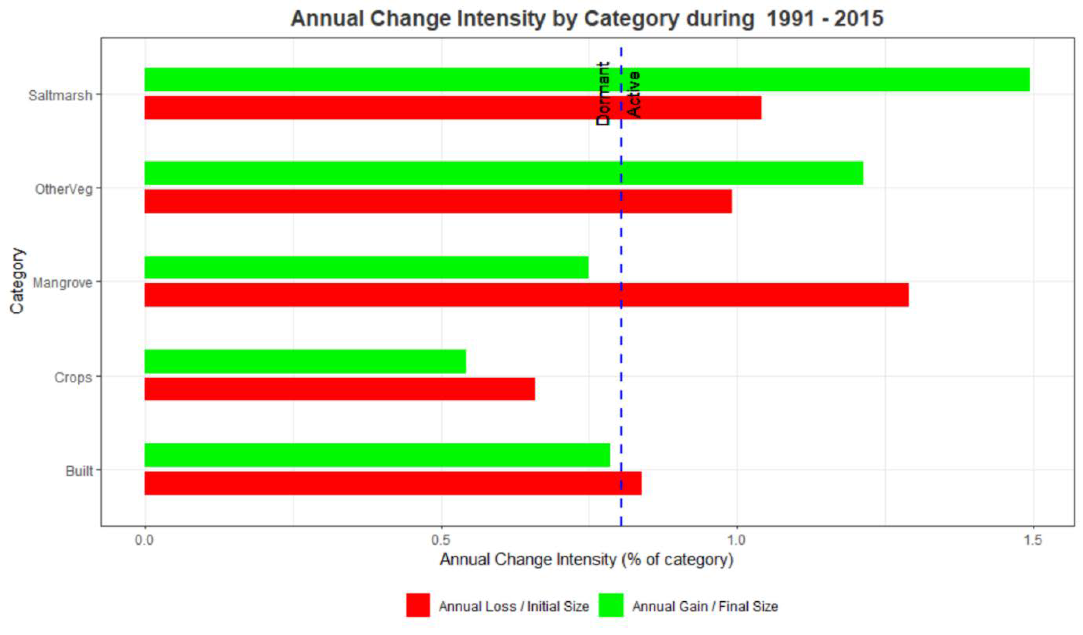
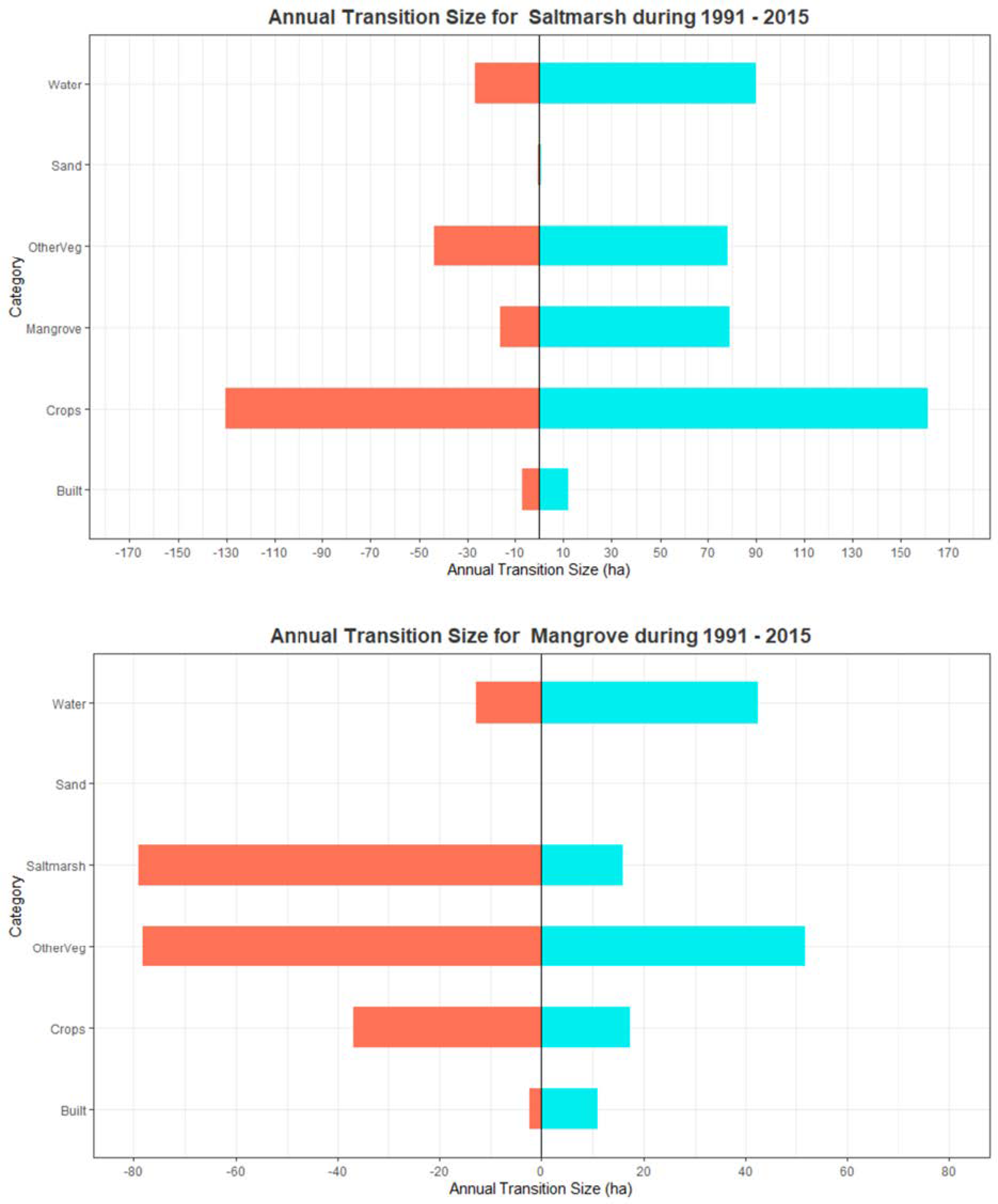
3.4. Land-Cover Change

We evaluated transitional patterns between land cover classes by grouping all regions together and comparing the earliest map of the time series (1991) to the latest (2015). Total afforestation and deforestation rates for mangroves are 0.75% and 1.3% annually, respectively. Saltmarsh experienced a higher rate of increase at 1.5% and a slightly lower rate of decline at 1.1%. (Figure 5). Saltmarsh ecosystems are actively both gaining and losing area; although, there is a clear tendency for gains (which is expected due to the rapid increase in saltmarsh extension in VIC). Mangroves on the other hand are only systematically losing area, as gain intensity is below the uniform change threshold (blue dashed vertical line, Figure 5) and can be considered dormant (or expected due to random processes; [70]).
Moreover, we evaluated the annual land cover change for saltmarsh and mangroves (Figure 6). Saltmarsh ecosystems experience higher systematic gains than losses through all the other categories, including “Cropland” (+161 vs. −130 ha annually), “Water” (+90 vs. −28 ha annually), “Other Vegetation” (+78 vs. −24 ha annually), and “Mangroves” (+79 ha vs. −16 ha annually).
On the other hand, mangrove ecosystems are consistently losing to all categories but “Water” (+43 ha vs. −14 ha annually). They gain and lose the most area to the category “Other Vegetation” (+52 ha vs. −77 ha annually), followed by “Saltmarsh” (+16 ha vs. −79 ha annually) and “Cropland” (+17 ha vs. −37 ha annually).

4. Discussion

In this study, we developed a time-series of ten medium resolution (30 m) land-cover maps between 1991 and 2015 for the coastal areas of south-eastern Australia, with a special focus on mangrove and saltmarsh ecosystems. We found that mangrove ecosystems are declining in south-eastern Australia (−1148 ha or 7.6%), while saltmarshes have experienced an overall increase (+4157 ha or 20.3%) over the 24-year period. A hotspot for these changes is Lake Wellington (Gippsland, VIC), which has experienced extensive conversion from freshwater wetlands to saltmarsh between 1999 and 2006 due to higher salinity conditions.
We tested the addition of two physical variables (SRTM and DistW) to our RF models and determined that the best model was the one using spectral bands and indices in combination with the two physical variables. The mangrove and saltmarsh maps produced in this study had an overall User Accuracy of 0.82–0.95 and 0.81–0.87 (for mangrove and saltmarsh, respectively) and an overall Producer Accuracy of 0.71–0.88 and 0.24–0.87 (for mangrove and saltmarsh, respectively) (Table 5 and Table S4). These values are consistent with other studies using similar methodology for mapping coastal wetlands in Australia [13], Brazil [40], Mozambique [32], and Mexico [71]. Furthermore, the high overall accuracy of our estimates (~90%) at the two time-steps where the models were created (2006 and 2013) provides the necessary confidence in the validity of the maps and their role in understanding coastal wetlands land-use change in south-eastern Australia.

4.1. Accuracy Assessment

To test the individual performance of the physical variables (SRTM height and DistW), we created 4 RF models with different combinations of variables: (1) Spectral; (2) Spectral + DistW; (3) Spectral + SRTM; and (4) Spectral + DistW + SRTM. Using OA, kappa statistics and class-specific accuracies (Table 4) we determined that the best model was model (4), which included spectral bands (blue, green, red, NIR, SWIR1 and SWIR2), spectral indices (NDVI, MNDWI, and MMRI) and the two physical indices (SRTM and DistW). Our classes of interest (mangrove and saltmarsh ecosystems) showed above average improvement in overall accuracy (Table 4). This is most likely due to the fact that these ecosystems can be considered mature vegetation stands, and have very low growth rates in south-eastern Australia, due to the cold climate [48]. Therefore, they are unlikely to show variability in canopy height through time and will not be negatively affected by the addition of SRTM as a variable, as SRTM’s vertical error is likely higher than the possible growth of these ecosystems over the study period [72]).
Producer and User Accuracy is consistently higher for mangroves than it is for saltmarsh (see Table 5). This is consistent with other studies that have performed similar classifications in coastal wetlands [71,73,74]. Several Ecological Vegetation Classes (EVCs) with different floristic and structural properties have been identified for saltmarsh ecosystems in the south-eastern coast of Australia [75,76]. In this study, we decided to combine all EVCs for saltmarsh ecosystems into only one class. As we are combining saltmarshes as spectrally and structurally different as woody succulent shrubs (e.g., Tecticornia arbuscula and Salicornia quinqueflora), rushes (Juncus kraussii), or grasses (e.g., Distichlis distichophylla), we expected a detrimental effect on overall accuracy of saltmarsh predictions due to the spectral differences they present [77]. On the other hand, mangrove ecosystems in the south-eastern coast of Australia are usually dominated by only one species (Avicennia marina) and therefore we expected the higher overall accuracies for this class that we found.
While Producer Accuracy for saltmarsh ecosystems is almost 0.8 in VIC, it is below 0.5 in NSW after applying the post-classification filters. We believe the main reason for this is that saltmarsh in the north of NSW is mainly composed of salt tolerant graminoids (such as Juncus kraussii) very similar to pastureland or crops. Indeed, the Producer Accuracy in the Northern Rivers section (NSW) is 0.24, while it is closer to 0.6 in the Central Coast (NSW). Moreover, the use of proportional samples in Random Forest algorithms tends to produce maps with lower producer accuracy for the classes with the lower number of samples [60]; in our case, the class “Crops” outbalance the class “Saltmarsh” in a 18 to 1 proportion in NSW (see Table S1). Others have used an equal number of samples to overcome this issue (see [32,40]). However, Millard and Richardson [60] warn us of the importance of carefully selecting training data so that landscape proportions are maintained. They found that when an equal number of training data samples were allocated for each class, the classes that were over-represented in the training sample were also over-represented in the predicted classification and vice versa. To verify this pattern (although not shown in this study), we also performed our analysis using an equal number of samples for each class (n = 2000) and found that, while overall coastal wetland accuracy tends to improve, mangrove and saltmarsh predictions were more than twice the size of our training regions. Nevertheless, the high User Accuracy for saltmarsh ecosystems in NSW (over 0.82) indicates that, while our model is not predicting very well all the areas where saltmarsh is present in NSW, we can be quite certain of the areas predicted.
Additionally, we demonstrated that the two post-classification filters applied in this study improve overall accuracy of coastal wetlands detection (Table 5). They provide a significant increase of User Accuracy across all regions of interest (up to 16%), while maintaining or slightly decreasing Producer Accuracy. Only a few other studies [32,40] have performed similar post-classification filters for mangrove detection. However, they did not demonstrate empirically the efficacy of these filters.

4.2. Mangrove and Saltmarsh Distribution

We show that mangrove ecosystems in the south-eastern coast of Australia have lost an area of 1148 ha (7.6%) over the 24 years period between 1991 and 2015. The major mangrove losses in terms of area can be found in Port Stephens estuary (Central Coast, NSW; Figure 3c) and Lake Wellington (Gippsland, VIC). The causes for mangrove dieback in Port Stephens are unclear but point to extreme weather events (hail damage [78]), and human development (upgrade of a highway that included the removal of 47 hectares of vegetation and affected mangroves and saltmarsh around Karuah River Nature Reserve; [79]). However, mangrove losses in Lake Wellington are likely produced by noise in our models, as Boon et al. [23] reported minimal presence of mangroves in the surroundings of the lake.
On the other hand, saltmarsh experienced an overall increase of 4157 ha (20.3%), most of which happened between 1999 and 2006 (Figure 2). Several hotspots for this rapid increase have been recognised from comparing the 1991 and 2015 distribution maps. Lake Wellington (Gippsland, VIC) is the most prominent one and has experienced an extensive increase in saltmarsh area (Figure 4c), accounting for nearly 75% of the total saltmarsh expansion (nearly 3000 ha, Figure 2). Since the permanent artificial opening of the lake to the sea in 1889 [80], Lake Wellington has experienced rapid fluctuations in salinity that have transformed the waters from fresh/brackish to saline, especially during drought years [81]. These transformations have caused a transition from freshwater vegetation to saltmarsh. Moreover, in 1998 (one year before the start of the rapid saltmarsh increase), there were extreme storm events associated with big floods in the area that pushed exceedingly large amounts of salt from the more saline Lake Reeve into the system, with the consequent dieback of predominant freshwater wetlands at the time [81]. Since then, saltmarsh coverage has remained constant around the lake (Figure 2) and it is likely to remain that way due to higher salinities in the lake correlated with the impacts of more frequent extreme weather events associated with climate change, like intensified drought conditions [10,82].
Other hotspots of saltmarsh expansion include small embayments around the western coast of Port Phillip Bay (Central Bays, VIC; Figure S1a), which have experienced similar droughts that have permitted the advancement of saltmarsh to cover previously known water sources (Figure S1c in supplementary). Moreover, we managed to capture the performance of several restoration projects in the north-western coast of Port Phillip Bay [17,83,84], with over 60 ha (according to our maps) of area reconverted from salt ponds or water management facilities to saltmarsh ecosystems (Figure S1b). However, there are some limitations with our models, as some of that increase has been associated with rapid expansion of Phragmites reed (especially in interior lakes of the western coast of Port Phillip Bay in Victoria, see Reedy Lake in Figure S1d and [85]), a rapidly growing freshwater grass that can live in brackish waters and which is spectrally similar to other, often adjacent, saltmarsh graminoids [77].
We also show that higher rates of increase can be found for saltmarsh (near 1.5% annually; Figure 5) than for mangroves (0.75% annually; Figure 5). Moreover, higher annual change rates for both mangrove and saltmarsh can be found in NSW compared to VIC (Figure S2), which could be a consequence of the lower accuracy numbers for both classes in NSW (Table 5). We then compared these intensities in change with the expected uniform change in the study area and determined that, while both saltmarsh accretion and decline are considered active, only mangrove declines are. Annual mangrove accretion is below the uniform change threshold and, consequently, more likely caused by random processes [70]. Therefore, we can assume that mangrove ecosystems are systematically losing area in the south-eastern coast of Australia over the time period analysed, which has been supported by a number of studies in the region [15,18,23].

4.3. Land-Cover Change

Finally, we evaluated the annual land cover change for saltmarsh and mangroves (Figure 6). Saltmarsh ecosystems gain and lose the most area to the category “Cropland” (+161 vs. −130 ha annually). As we expect saltmarsh and cropland to share spectral traits (especially in northern NSW, due to the aforementioned grassy nature of predominant saltmarshes in the area), we explored the location of these changes to determine if they are caused by systematic changes or random mislabelling of saltmarsh ecosystems. We expected a great proportion of the pixels to be due to true swap between classes, especially after the two post-classification filters we applied. Indeed, we found several hotspots of systematic change from saltmarsh to pastureland. These spots are often found in the fringe between saltmarsh and livestock grazing areas with no fencing, and result in the degradation of saltmarsh ecosystems to the point where we detect them as “Crops” in our maps (Figure S3). However, this systematic change is only a small percentage (~5%) of the total swap between these two classes. We then assume that most of the swap between these two classes is due to random mislabelling and indeed, we observe that saltmarsh ecosystems have the most omission and commission errors to the Crops category (see confusion matrix, Table S2).
Similarly, mangroves gain and lose the most area to the category “Other Vegetation” (+52 ha vs. −77 ha annually). Again, we expect a high proportion of these changes to be due to random mislabelling of mangrove ecosystems, which is confirmed by the confusion matrix (Table S2, mangrove ecosystems have the most omission and commission errors to the Other Vegetation category). These two problems are common among mangrove and saltmarsh distribution studies due to the spectral similarity between saltmarsh graminoids and pastureland [77], and mangroves and other evergreen vegetation [30,33].
We also notice that both ecosystems have higher gains than losses to the Built category (around −12 ha annually for both mangroves and saltmarsh). However, using high resolution imagery from Google Earth we determined that 100% of the observed area being transformed from “Built” to the “Mangrove” and “Saltmarsh” categories is due to previously undetected water and sand pixels that are being predicted as “Built”. This is caused by the generally low spectral reflectance typical of these 3 categories [86]. On the other hand, while some of the change from “Mangrove” and “Saltmarsh” to “Built” is also due to undetected water and sand pixels, we established that approximately 2 ha of coastal wetlands are being lost to coastal development annually, including ports (Figure S4a,b), aquaculture facilities (Figure S4c), and residential areas (Figure S4d).
Moreover, we found that mangrove and saltmarsh ecosystems gain more area from water (43 ha and 90 ha annually, respectively) than they lose (14 ha and 28 ha annually, respectively). This is contrary to what we would expect under the current climate change conditions and, indeed, to what others have reported in the region [25]. Using high resolution imagery from Google Earth, we determined that, even though some of this change is truly associated with mangrove expansion into water, the majority comes from canopy and coverage growth of sparse mangrove trees in the fringe between mangrove and water (Figure 3d).
Furthermore, another surprising land cover change was mangroves losing more area to saltmarsh than they gained (Figure 6). The opposite effect (encroachment of mangrove ecosystems into saltmarshes) has been well documented in several estuaries and embayments of the south-eastern coast of Australia [15,25,87,88]. A hotspot area for these two unforeseen changes is Westernport in VIC (Figure 3d and Figure 4d). Here, both Rogers et al. [87] and Whitt et al. [25] reported general encroachment of mangroves into saltmarsh ecosystems using very high-resolution aerial imagery. It is likely that their reported general encroachment of mangroves into saltmarsh ecosystems is less extensive than the resolution of our pixels (30 m). We established that the area that is being modelled as change from mangrove to saltmarsh is actually the fringe where both ecosystems occur simultaneously. Therefore, instead of actual swap from mangrove to saltmarsh, the changes we observe are likely due to other factors like intensified drought conditions [82], which can alter mangroves structure and spectral traits, potentially making them more similar to saltmarsh ecosystems [89], or cyclical spatio-temporal expansion/contraction of mangrove and saltmarsh ecosystems as reported by Rodriguez et al. [90] in Florida, USA. Moreover, on a similar study in the Texas Gulf Coast, Armitage et al. [91] concluded that the saltmarsh to mangrove shift is not as widespread when analysed at a larger, regional level using medium resolution satellite imagery (Landsat 5 TM) when compared to small-scale studies.

4.4. Potential Data Applications and Management Implications

Coastal change monitoring has become a critically essential tool for assessing the effects that rapid increases of Australian population along the coast have on coastal wetlands both directly (i.e., high rates of agricultural expansion and urban growth [11]), and indirectly (i.e., climate change and the associated impacts of sea level rise [10]). The high accuracy and temporal resolution of our maps make them particularly suitable inputs into studies spanning a wide range of purposes, including carbon sequestration projects seeking to gain carbon credits for mangrove and saltmarsh rehabilitation under the impacts of climate change related issues [10]. Although some care must be taken when using these maps, they can be used to provide a broad understanding of the spatial and temporal distribution of these important coastal ecosystems to inform management.
As an example, areas like Lake Wellington (Gippsland, VIC) could become the focus of conservation projects to take advantage of the rapid increase of saltmarsh extent observed in the area. Similarly, areas of widespread losses of mangrove and saltmarsh ecosystems, such as Port Stephens estuary (Central Coast, NSW) and Westernport (Central Bays, VIC), could be the focus of restoration projects to recover coastal wetland area lost by extreme weather events and other anthropogenic related threats.

5. Conclusions

Our results provide a comprehensive set of coastal land-cover uses and land change information for the south-eastern coast of Australia, with a focus on coastal wetland (mangrove and saltmarsh) ecosystems. We have demonstrated that the addition of SRTM and Distance to Water layers, and spatial and temporal post-classification filters improves overall accuracy of coastal wetlands detection using Random Forest models. While there are a growing number of studies investigating land cover changes for coastal wetland ecosystems, we are, to the best of our knowledge, the first to study the transitional patterns of coastal wetlands into other land uses at the state level in Australia. The resultant maps obtained in this study have the potential to provide local and statewide managers with an effective method for quantifying the gains and losses of coastal wetlands in south-eastern Australia.

Supplementary Materials

The following are available online at https://0-www-mdpi-com.brum.beds.ac.uk/article/10.3390/rs13081450/s1, Figures S1–S4, Tables S1–S4.

Author Contributions

Conceptualization, A.N., M.Y. and D.I.; Formal analysis, A.N.; Funding acquisition, P.I.M., E.N. and D.I.; Investigation, A.N.; Methodology, A.N.; Project administration, D.I.; Supervision, M.Y., P.I.M., E.N. and D.I.; Writing—original draft, A.N.; Writing—review and editing, M.Y., P.I.M., E.N. and D.I. All authors have read and agreed to the published version of the manuscript.

Funding

This study is part of the Mapping Ocean Wealth project from The Nature Conservancy’s Great Southern Seascapes program and supported by The Thomas Foundation, HSBC Australia, the Ian Potter Foundation, and Victorian and New South Wales governments including Parks Victoria, Department of Environment Land, Water, and Planning, Victorian Fisheries Authority, New South Wales Office of Environment and Heritage, and New South Wales Department of Primary Industries. Funding was also provided by an Australian Research Council Linkage Project (LP160100242).

Data Availability Statement

Conflicts of Interest

The authors declare no conflict of interest. The funders had no role in the design of the study; in the collection, analyses, or interpretation of data; in the writing of the manuscript, or in the decision to publish the results.

References

  1. Alongi, D.M. Mangrove forests: Resilience, protection from tsunamis, and responses to global climate change. Estuar. Coast. Shelf Sci. 2008, 76, 1–13. [Google Scholar] [CrossRef]
  2. Atwood, T.B.; Connolly, R.M.; Almahasheer, H.; Carnell, P.E.; Duarte, C.M.; Lewis, C.J.E.; Irigoien, X.; Kelleway, J.J.; Lavery, P.S.; Macreadie, P.I. Global patterns in mangrove soil carbon stocks and losses. Nat. Clim. Chang. 2017, 7, 523. [Google Scholar] [CrossRef]
  3. Das, S.; Vincent, J.R. Mangroves protected villages and reduced death toll during Indian super cyclone. Proc. Natl. Acad. Sci. USA 2009, 106, 7357–7360. [Google Scholar] [CrossRef] [PubMed] [Green Version]
  4. Hemminga, M.A.; Duarte, C.M. Seagrass Ecology; Cambridge University Press: Cambridge, UK, 2000. [Google Scholar]
  5. Mcleod, E.; Chmura, G.L.; Bouillon, S.; Salm, R.; Björk, M.; Duarte, C.M.; Lovelock, C.E.; Schlesinger, W.H.; Silliman, B.R. A blueprint for blue carbon: Toward an improved understanding of the role of vegetated coastal habitats in sequestering CO2. Front. Ecol. Environ. 2011, 9, 552–560. [Google Scholar] [CrossRef] [Green Version]
  6. Clark, G.F.; Johnston, E.L. Coasts. Australia State of the Environment; Government Department of the Environment and Energy: Canberra, Australia, 2016. Available online: https://soe.environment.gov.au/theme/coasts (accessed on 6 April 2021).
  7. Richards, D.R.; Friess, D.A. Rates and drivers of mangrove deforestation in Southeast Asia, 2000–2012. Proc. Natl. Acad. Sci. USA 2016, 113, 344–349. [Google Scholar] [CrossRef] [Green Version]
  8. Duke, N.C.; Kovacs, J.M.; Griffiths, A.D.; Preece, L.; Hill, D.J.E.; van Oosterzee, P.; Mackenzie, J.; Morning, H.S.; Burrows, D. Large-scale dieback of mangroves in Australia’s Gulf of Carpentaria: A severe ecosystem response, coincidental with an unusually extreme weather event. Mar. Freshw. Res. 2017, 68, 1816–1829. [Google Scholar] [CrossRef]
  9. Lugo, A.E. Effects and outcomes of Caribbean hurricanes in a climate change scenario. Sci. Total Environ. 2000, 262, 243–251. [Google Scholar] [CrossRef]
  10. Ward, R.D.; Friess, D.A.; Day, R.H.; MacKenzie, R.A. Impacts of climate change on mangrove ecosystems: A region by region overview. Ecosyst. Health Sustain. 2016, 2. [Google Scholar] [CrossRef] [Green Version]
  11. Zann, L.P. The eastern Australian region: A dynamic tropical/temperate biotone. Mar. Pollut. Bull. 2000, 41, 188–203. [Google Scholar] [CrossRef]
  12. Montreal Process Implementation Group for Australia and National Forest Inventory Steering Committee. Australia’s State of the Forests Report 2018; ABARES: Canberra, Australia, 2018. [Google Scholar]
  13. Lymburner, L.; Bunting, P.; Lucas, R.; Scarth, P.; Alam, I.; Phillips, C.; Ticehurst, C.; Held, A. Mapping the multi-decadal mangrove dynamics of the Australian coastline. Remote Sens. Environ. 2020, 238, 111185. [Google Scholar] [CrossRef]
  14. Act, E. Environment Protection and Biodiversity Conservation Act; ABARES: Canberra, Australia, 1999. [Google Scholar]
  15. Saintilan, N.; Williams, R. Short Note: The decline of saltmarsh in southeast Australia: Results of recent surveys. Wetl. Aust. 2010, 18. [Google Scholar] [CrossRef]
  16. Sinclair, S.; Boon, P.I. Changes in the area of coastal marsh in Victoria since the mid19th century. Cunninghamia 2012, 12, 153–176. [Google Scholar]
  17. Gulliver, A.; Carnell, P.E.; Trevathan-Tackett, S.M.; Duarte de Paula Costa, M.; Masqué, P.; Macreadie, P.I. Estimating the potential blue carbon gains from tidal marsh rehabilitation: A case study from south eastern Australia. Front. Mar. Sci. 2020, 7, 403. [Google Scholar] [CrossRef]
  18. Hurst, T. Restoration of Temperate Mangrove Ecosystems; Deakin University: Melbourne, Australia, 2018. [Google Scholar]
  19. Russell, K. NSW Northern Rivers Estuary Habitat Mapping-Final Analysis Report; NSW Department of Primary Industries: Port Stephens, Australia, 2005. [Google Scholar]
  20. Adame, M.; Hermoso, V.; Perhans, K.; Lovelock, C.; Herrera-Silveira, J. Selecting cost-effective areas for restoration of ecosystem services. Conserv. Biol. 2015, 29, 493–502. [Google Scholar] [CrossRef] [PubMed] [Green Version]
  21. Hardisky, M.; Gross, M.; Klemas, V. Remote sensing of coastal wetlands. Bioscience 1986, 36, 453–460. [Google Scholar] [CrossRef]
  22. Worthington, T.; Spalding, M. Mangrove restoration potential: A global map highlighting a critical opportunity. Apollo 2018. [Google Scholar] [CrossRef]
  23. Boon, P.; Allen, T.; Brook, J.; Carr, G.; Frood, D.; Harty, C.; Hoye, J.; McMahon, A.; Mathews, S.; Rosengren, N. Victorian Saltmarsh Study. Mangroves and Coastal Saltmarsh of Victoria: Distribution, Condition, Threats and Management; Institute for Sustainability and Innovation, Victoria University: Melbourne, Australia, 2011. [Google Scholar]
  24. Creese, R.; Glasby, T.; West, G.; Gallen, C. Mapping the habitats of NSW estuaries. Nelson Bay NSW 2009, 113, 1837–2112. [Google Scholar]
  25. Whitt, A.A.; Coleman, R.; Lovelock, C.E.; Gillies, C.; Ierodiaconou, D.; Liyanapathirana, M.; Macreadie, P.I. March of the mangroves: Drivers of encroachment into southern temperate saltmarsh. Estuar. Coast. Shelf Sci. 2020, 240, 106776. [Google Scholar] [CrossRef]
  26. Dustin, M.C. Monitoring Parks with Inexpensive UAVs: Cost Benefits Analysis for Monitoring and Maintaining Parks Facilities; University of Southern California: Los Angeles, CA, USA, 2015. [Google Scholar]
  27. Mumby, P.; Green, E.; Edwards, A.; Clark, C. The cost-effectiveness of remote sensing for tropical coastal resources assessment and management. J. Environ. Manag. 1999, 55, 157–166. [Google Scholar] [CrossRef]
  28. Giri, C. Observation and Monitoring of Mangrove Forests Using Remote Sensing: Opportunities and Challenges. Remote Sens. 2016, 8, 783. [Google Scholar] [CrossRef] [Green Version]
  29. Kuenzer, C.; Bluemel, A.; Gebhardt, S.; Quoc, T.V.; Dech, S. Remote Sensing of Mangrove Ecosystems: A Review. Remote Sens. 2011, 3, 878–928. [Google Scholar] [CrossRef] [Green Version]
  30. Pham, T.D.; Yokoya, N.; Bui, D.T.; Yoshino, K.; Friess, D.A. Remote Sensing Approaches for Monitoring Mangrove Species, Structure, and Biomass: Opportunities and Challenges. Remote Sens. 2019, 11, 230. [Google Scholar] [CrossRef] [Green Version]
  31. Bunting, P.; Rosenqvist, A.; Lucas, R.M.; Rebelo, L.M.; Hilarides, L.; Thomas, N.; Hardy, A.; Itoh, T.; Shimada, M.; Finlayson, C.M. The Global Mangrove WatchA New 2010 Global Baseline of Mangrove Extent. Remote Sens. 2018, 10, 1669. [Google Scholar] [CrossRef] [Green Version]
  32. Fatoyinbo, T.E.; Simard, M.; Washington-Allen, R.A.; Shugart, H.H. Landscape-scale extent, height, biomass, and carbon estimation of Mozambique’s mangrove forests with Landsat ETM+ and Shuttle Radar Topography Mission elevation data. J. Geophys. Res. Biogeosci. 2008, 113. [Google Scholar] [CrossRef]
  33. Giri, C.; Ochieng, E.; Tieszen, L.L.; Zhu, Z.; Singh, A.; Loveland, T.; Masek, J.; Duke, N. Status and distribution of mangrove forests of the world using earth observation satellite data. Glob. Ecol. Biogeogr. 2011, 20, 154–159. [Google Scholar] [CrossRef]
  34. Heumann, B.W. Satellite remote sensing of mangrove forests: Recent advances and future opportunities. Prog. Phys. Geogr. 2011, 35, 87–108. [Google Scholar] [CrossRef]
  35. Wulder, M.A.; White, J.C.; Loveland, T.R.; Woodcock, C.E.; Belward, A.S.; Cohen, W.B.; Fosnight, E.A.; Shaw, J.; Masek, J.G.; Roy, D.P. The global Landsat archive: Status, consolidation, and direction. Remote Sens. Environ. 2016, 185, 271–283. [Google Scholar] [CrossRef] [Green Version]
  36. Calderón-Loor, M.; Hadjikakou, M.; Bryan, B.A. High-resolution wall-to-wall land-cover mapping and land change assessment for Australia from 1985 to 2015. Remote Sens. Environ. 2021, 252, 112148. [Google Scholar] [CrossRef]
  37. Giri, C.; Long, J.; Abbas, S.; Murali, R.M.; Qamer, F.M.; Pengra, B.; Thau, D. Distribution and dynamics of mangrove forests of South Asia. J. Environ. Manag. 2015, 148, 101–111. [Google Scholar] [CrossRef] [PubMed]
  38. Murray, N.J.; Phinn, S.R.; DeWitt, M.; Ferrari, R.; Johnston, R.; Lyons, M.B.; Clinton, N.; Thau, D.; Fuller, R.A. The global distribution and trajectory of tidal flats. Nature 2019, 565, 222–225. [Google Scholar] [CrossRef]
  39. Song, X.-P.; Hansen, M.C.; Stehman, S.V.; Potapov, P.V.; Tyukavina, A.; Vermote, E.F.; Townshend, J.R. Global land change from 1982 to 2016. Nature 2018, 560, 639–643. [Google Scholar] [CrossRef]
  40. Diniz, C.; Cortinhas, L.; Nerino, G.; Rodrigues, J.; Sadeck, L.; Adami, M.; Souza-Filho, P.W.M. Brazilian mangrove status: Three decades of satellite data analysis. Remote Sens. 2019, 11, 808. [Google Scholar] [CrossRef] [Green Version]
  41. Gupta, K.; Mukhopadhyay, A.; Giri, S.; Chanda, A.; Majumdar, S.D.; Samanta, S.; Mitra, D.; Samal, R.N.; Pattnaik, A.K.; Hazra, S. An index for discrimination of mangroves from non-mangroves using LANDSAT 8 OLI imagery. MethodsX 2018, 5, 1129–1139. [Google Scholar] [CrossRef]
  42. Wen, L.; Hughes, M. Coastal wetland mapping using ensemble learning algorithms: A comparative study of bagging, boosting and stacking techniques. Remote Sens. 2020, 12, 1683. [Google Scholar] [CrossRef]
  43. Rogan, J.; Franklin, J.; Stow, D.; Miller, J.; Woodcock, C.; Roberts, D. Mapping land-cover modifications over large areas: A comparison of machine learning algorithms. Remote Sens. Environ. 2008, 112, 2272–2283. [Google Scholar] [CrossRef]
  44. Heumann, B.W. An Object-Based Classification of Mangroves Using a Hybrid Decision Tree-Support Vector Machine Approach. Remote Sens. 2011, 3, 2440–2460. [Google Scholar] [CrossRef] [Green Version]
  45. Bwangoy, J.R.B.; Hansen, M.C.; Roy, D.P.; De Grandi, G.; Justice, C.O. Wetland mapping in the Congo Basin using optical and radar remotely sensed data and derived topographical indices. Remote Sens. Environ. 2010, 114, 73–86. [Google Scholar] [CrossRef]
  46. Renno, C.D.; Nobre, A.D.; Cuartas, L.A.; Soares, J.V.; Hodnett, M.G.; Tomasella, J.; Waterloo, M.J. HAND, a new terrain descriptor using SRTM-DEM: Mapping terra-firme rainforest environments in Amazonia. Remote Sens. Environ. 2008, 112, 3469–3481. [Google Scholar] [CrossRef]
  47. Wolanski, E.; Brinson, M.M.; Cahoon, D.R.; Perillo, G.M. Coastal Wetlands: A synthesis. In Coastal Wetlands an Integrated Ecosystem Approach; Elsevier: Amsterdam, The Netherlands, 2009; pp. 1–62. [Google Scholar]
  48. Macnae, W. Mangroves in eastern and southern Australia. Aust. J. Bot. 1966, 14, 67–104. [Google Scholar] [CrossRef]
  49. Farr, T.G.; Rosen, P.A.; Caro, E.; Crippen, R.; Duren, R.; Hensley, S.; Kobrick, M.; Paller, M.; Rodriguez, E.; Roth, L. The shuttle radar topography mission. Rev. Geophys. 2007, 45. [Google Scholar] [CrossRef] [Green Version]
  50. Vandervalk, A.G.; Attiwill, P.M. Decomposition of leaf and root litter of Avicennia-marina at Westernport Bay, Victoria, Australia. Aquat. Bot. 1984, 18, 205–221. [Google Scholar] [CrossRef]
  51. Adam, P.; Wilson, N.; Huntley, B. The phytosociology of coastal saltmarsh vegetation in New South Wales. Wetl. Aust. 2010, 7. [Google Scholar] [CrossRef]
  52. Li, F.; Jupp, D.L.; Reddy, S.; Lymburner, L.; Mueller, N.; Tan, P.; Islam, A. An evaluation of the use of atmospheric and BRDF correction to standardize Landsat data. IEEE J. Sel. Top. Appl. Earth Obs. Remote Sens. 2010, 3, 257–270. [Google Scholar] [CrossRef]
  53. Zhu, Z.; Woodcock, C.E. Object-based cloud and cloud shadow detection in Landsat imagery. Remote Sens. Environ. 2012, 118, 83–94. [Google Scholar] [CrossRef]
  54. Foga, S.; Scaramuzza, P.L.; Guo, S.; Zhu, Z.; Dilley, R.D., Jr.; Beckmann, T.; Schmidt, G.L.; Dwyer, J.L.; Hughes, M.J.; Laue, B. Cloud detection algorithm comparison and validation for operational Landsat data products. Remote Sens. Environ. 2017, 194, 379–390. [Google Scholar] [CrossRef] [Green Version]
  55. Gorelick, N.; Hancher, M.; Dixon, M.; Ilyushchenko, S.; Thau, D.; Moore, R. Google Earth Engine: Planetary-scale geospatial analysis for everyone. Remote Sens. Environ. 2017, 202, 18–27. [Google Scholar] [CrossRef]
  56. Held, A.; Ticehurst, C.; Lymburner, L.; Williams, N. High resolution mapping of tropical mangrove ecosystems using hyperspectral and radar remote sensing. Int. J. Remote Sens. 2003, 24, 2739–2759. [Google Scholar] [CrossRef]
  57. Navarro, A.; Young, M.; Allan, B.; Carnell, P.; Macreadie, P.; Ierodiaconou, D. The application of Unmanned Aerial Vehicles (UAVs) to estimate above-ground biomass of mangrove ecosystems. Remote Sens. Environ. 2020, 242, 111747. [Google Scholar] [CrossRef]
  58. State Government of NSW and Department of Planning Industry and Environment. NSW Landuse 2007; Department of Planning, Industry and Environment: Parramatta, Australia, 2010.
  59. State Government of VIC and Department of Environment Land Water and Planning. VIC Landuse 2006; Department of Environment Land Water and Planning: Melbourne, Australia, 2006.
  60. Millard, K.; Richardson, M. On the Importance of Training Data Sample Selection in Random Forest Image Classification: A Case Study in Peatland Ecosystem Mapping. Remote Sens. 2015, 7, 8489–8515. [Google Scholar] [CrossRef] [Green Version]
  61. Young, N.E.; Anderson, R.S.; Chignell, S.M.; Vorster, A.G.; Lawrence, R.; Evangelista, P.H. A survival guide to Landsat preprocessing. Ecology 2017, 98, 920–932. [Google Scholar] [CrossRef] [Green Version]
  62. Breiman, L. Random forests. Mach. Learn. 2001, 45, 5–32. [Google Scholar] [CrossRef] [Green Version]
  63. Liaw, A.; Wiener, M. Classification and regression by randomForest. R News 2002, 2, 18–22. [Google Scholar]
  64. Rouse, J.; Haas, R.H.; Schell, J.A.; Deering, D.W. Monitoring vegetation systems in the Great Plains with ERTS. NASA Spec. Publ. 1974, 351, 309. [Google Scholar]
  65. Xu, H.Q. Modification of normalised difference water index (NDWI) to enhance open water features in remotely sensed imagery. Int. J. Remote Sens. 2006, 27, 3025–3033. [Google Scholar] [CrossRef]
  66. Bivand, R.; Rundel, C. rgeos: Interface to Geometry Engine—Open Source (‘GEOS’). 2020. Available online: https://cran.r-project.org/web/packages/rgeos/index.html (accessed on 7 April 2021).
  67. Kuhn, M. Building predictive models in R using the caret package. J. Stat. Softw. 2008, 28, 1–26. [Google Scholar] [CrossRef] [Green Version]
  68. Ferri, C.; Hernández-Orallo, J.; Modroiu, R. An experimental comparison of performance measures for classification. Pattern Recognit. Lett. 2009, 30, 27–38. [Google Scholar] [CrossRef]
  69. Pontius, R.G., Jr.; Khallaghi, S. Intensity. Analysis: Intensity of Change for Comparing Categorical Maps from Sequential Intervals. 2019. Available online: https://cran.r-project.org/web/packages/intensity.analysis/index.html (accessed on 7 April 2021).
  70. Pontius, R.G., Jr.; Shusas, E.; McEachern, M. Detecting important categorical land changes while accounting for persistence. Agric. Ecosyst. Environ. 2004, 101, 251–268. [Google Scholar] [CrossRef]
  71. Berlanga-Robles, C.A.; Ruiz-Luna, A.; Bocco, G.; Vekerdy, Z. Spatial analysis of the impact of shrimp culture on the coastal wetlands on the Northern coast of Sinaloa, Mexico. Ocean Coast. Manag. 2011, 54, 535–543. [Google Scholar] [CrossRef]
  72. Hirt, C.; Filmer, M.; Featherstone, W. Comparison and validation of the recent freely available ASTER-GDEM ver1, SRTM ver4. 1 and GEODATA DEM−9S ver3 digital elevation models over Australia. Aust. J. Earth Sci. 2010, 57, 337–347. [Google Scholar] [CrossRef] [Green Version]
  73. Cardoso, G.F.; Souza, C.; Souza-Filho, P.W.M. Using spectral analysis of Landsat−5 TM images to map coastal wetlands in the Amazon River mouth, Brazil. Wetl. Ecol. Manag. 2014, 22, 79–92. [Google Scholar] [CrossRef]
  74. Rodrigues, S.W.P.; Souza-Filho, P.W.M. Use of multi-sensor data to identify and map tropical coastal wetlands in the Amazon of Northern Brazil. Wetlands 2011, 31, 11–23. [Google Scholar] [CrossRef]
  75. Oates, A.; Taranto, M. Vegetation Mapping of the Port Phillip and Westerport Region; Department of Natural Resources and Environment: East Melbourne, Australia, 2001. [Google Scholar]
  76. Department of Natural Resources and Environment. Victoria’s Native Vegetation Management: A Framework for Action; Department of Natural Resources and Environment: Melbourne, Australia, 2002. [Google Scholar]
  77. Schmidt, K.; Skidmore, A. Spectral discrimination of vegetation types in a coastal wetland. Remote Sens. Environ. 2003, 85, 92–108. [Google Scholar] [CrossRef]
  78. Elias, C. Hail Damage Likely Cause of Port Stephens Estuary Mangrove Dieback, DPI Say. Port Stephens Examiner 2019, January 23. Available online: https://www.portstephensexaminer.com.au/story/5832988/unlikely-cause-for-alarming-mangrove-dieback/ (accessed on 7 April 2021).
  79. Department of Environment and Conservation NSW. Avoiding and Offsetting Biodiversity Loss, Case Studies; Department of Environment and Conservation NSW: Sydney, Australia, 2013. [Google Scholar]
  80. Day, P.R. Lake Wellington Science Review; West Gippsland Catchment Management Authority: Traralgon, Australia, 2018. [Google Scholar]
  81. Ladson, A.; Hillemacher, M.; Treadwell, S. Lake Wellington Salinity: Investigation of Management Options. In Proceedings of the 34th World Congress of the International Association for Hydro-Environment Research and Engineering: 33rd Hydrology and Water Resources Symposium and 10th Conference on Hydraulics in Water Engineering, Brisbane Australia, 26 June–1 July 2011; p. 3207. [Google Scholar]
  82. Nicholls, N. The changing nature of Australian droughts. Clim. Chang. 2004, 63, 323–336. [Google Scholar] [CrossRef]
  83. Cheetham Salt. Historical Timeline; Cheetham Salt: Melbourne, Australia, 2013. [Google Scholar]
  84. Ecology Australia. Western Treatment Plan: Results of Monitoring of Saltmarsh Colonisation of the Western Lagoon to Mid 2012; Ecology Australia PTY Ltd.: Fairfield, Australia, 2012. [Google Scholar]
  85. Ecological Associates. Reedy Lake Vegetation Monitoring Final Report; Ecological Associates Report BX010–2-B Prepared for Corangamite Catchment Management Authority; Corangamite Catchment Management Authority: Colac, Australia, 2014. [Google Scholar]
  86. Yang, X.; Qin, Q.; Grussenmeyer, P.; Koehl, M. Urban surface water body detection with suppressed built-up noise based on water indices from Sentinel−2 MSI imagery. Remote Sens. Environ. 2018, 219, 259–270. [Google Scholar] [CrossRef]
  87. Rogers, K.; Saintilan, N.; Heijnis, H. Mangrove encroachment of salt marsh in Western Port Bay, Victoria: The role of sedimentation, subsidence, and sea level rise. Estuaries 2005, 28, 551–559. [Google Scholar] [CrossRef]
  88. Saintilan, N.; Wilson, N.C.; Rogers, K.; Rajkaran, A.; Krauss, K.W. Mangrove expansion and salt marsh decline at mangrove poleward limits. Glob. Chang. Biol. 2014, 20, 147–157. [Google Scholar] [CrossRef] [PubMed] [Green Version]
  89. Zhang, C.; Chen, K.; Liu, Y.; Kovacs, J.M.; Flores-Verdugo, F.; de Santiago, F.J.F. Spectral response to varying levels of leaf pigments collected from a degraded mangrove forest. J. Appl. Remote Sens. 2012, 6, 063501. [Google Scholar]
  90. Rodriguez, W.; Feller, I.C.; Cavanaugh, K.C. Spatio-temporal changes of a mangrove–saltmarsh ecotone in the northeastern coast of Florida, USA. Glob. Ecol. Conserv. 2016, 7, 245–261. [Google Scholar] [CrossRef]
  91. Armitage, A.R.; Highfield, W.E.; Brody, S.D.; Louchouarn, P. The contribution of mangrove expansion to salt marsh loss on the Texas Gulf Coast. PLoS ONE 2015, 10, e0125404. [Google Scholar] [CrossRef]
Figure 1. South-eastern coast of Australia. Figure includes the 5 sub-regions our study area was divided into: three in NSW (Northern Rivers, from Tweed Head to Manning River at Taree; Central Coast, from Manning River to Shoalhaven River at Nowra; and Southern Rivers, from Shoalhaven River to Cape Howe) and two in VIC (Gippsland, from Cape Howe to Powlett River at Kilcunda; and Central Bays, which include Westernport and Port Phillip Bay).
Remotesensing 13 01450 g001
Figure 2. Mangrove (a) and saltmarsh (b) area extent in ha for every region of interest and in total.
Remotesensing 13 01450 g002
Figure 3. Mangrove gains, losses, and persistence between 1991 and 2015 across the south-eastern coast of Australia (a), along with several zoomed-in examples (bd).
Remotesensing 13 01450 g003
Figure 4. Saltmarsh gains, losses, and persistence between 1991 and 2015 across the south-eastern coast of Australia (a), along with several zoomed-in examples (bd).
Remotesensing 13 01450 g004
Figure 5. Annual change intensity in terms of gains (in green, calculated as the size of each gross annual gain divided by the size of the category at the final time point of the interval) and losses (in red; calculated as the size of each gross annual loss divided by the size of the category at the initial time point of the interval). The dashed vertical line indicates the land categories that are relatively dormant (left of the line) versus active (right of the line) in terms of loss and gain between 1991 and 2015, by comparing these intensities with uniform change in the study area. For more information see Pontius and Khallaghi [69].
Remotesensing 13 01450 g005
Figure 6. Annual Land Cover change for saltmarsh (top) and mangrove (bottom) ecosystems from 1991 to 2015. Gains in blue to the right of the central line and loses in red to the left.
Remotesensing 13 01450 g006
Table 1. Set of physical variables and vegetation indices used for modelling land use maps used in our study.
TypeVariablesVariable SpecificationsReference
Spectral BandsBlue0.45–0.52 μm (L5)
0.452–0.512 μm (L8)
NA
Green0.52–0.60 μm (L5)
0.533–0.590 μm (L8)
Red0.63–0.69 μm (L5)
0.636–0.673 μm (L8)
Near Infrared (NIR)0.77–0.90 μm (L5)
0.851–0.879 μm (L8)
Short-wave Infrared (SWIR 1)1.55–1.75 μm (L5)
1.566–1.651 μm (L8)
Short-wave Infrared (SWIR 2)2.08–2.35 μm (L5)
2.107–2.294 μm (L8)
Spectral IndicesNormalised Difference Vegetation Index (NDVI) ρ N I R ρ R e d ρ N I R + ρ R e d Rouse et al. [64]
Modified Normalised Difference Water Index (MNDWI) ρ G r e e n ρ S W I R 1 ρ G r e e n + ρ S W I R 1 Xu [65]
Modular Mangrove Recognition Index (MMRI) | M N D W I | | N D V I | | M N D W I | + | N D V I | Diniz et al. [40]
PhysicalShuttle Radar Topography Mission (SRTM)NAFarr et al. [49]
Distance to Water (DistW)NACreated using the gDistance function within the rgeos package (Bivand and Rundel [66])
Table 2. Post-classification spatial filter applied to our land-use maps. It searches for uncommon (less than 5% of all pixels in the ground-truthed training datasets met these criteria) mangrove and saltmarsh patches and removes them according to the following excluding criteria.
ClassExcluding Criteria
Distance to WaterPatch Size
MangrovesAny<0.2 ha
>45 m (1 pixel)<1 ha
SaltmarshAny<0.5 ha
>120 m (4 pixels)<5 ha
Table 3. Post-classification temporal filter applied to our land-use maps. It searches for deviations in the central timestep of three consecutive maps and changes it according to the following rules.
Before Temporal FilterAfter Temporal Filter
Mapn−1MapnMapn+1Mapn−1MapnMapn+1
Class XNon-Class XClass XClass XClass XClass X
Class YClass XClass YClass YClass YClass Y
Table 4. Overall Accuracy (OA), Kappa statistics, and class specific balanced accuracies for Mangroves (MgA) and Saltmarsh (SmA) across all regions of interest for the 2006/Landsat 5 model after applying post-classification filters.
NSWVIC
Northern RiversCentral CoastSouthern RiversGippslandCentral Bays
OAKappaMgASmAOAKappaMgASmAOAKappaMgASmAOAKappaMgASmAOAKappaMgASmA
Spectral0.880.770.810.520.870.820.830.720.860.790.820.670.870.740.920.830.860.800.940.87
Spectral + DistW0.890.780.820.590.880.830.840.740.870.800.830.690.870.740.920.840.870.810.940.88
Spectral + SRTM0.890.790.830.550.880.840.870.780.870.800.840.730.880.760.940.850.880.830.940.92
Spectral + DistW + SRTM0.900.800.850.620.890.840.870.790.880.800.850.730.880.770.930.850.880.830.940.92
Table 5. User (UA) and Producer Accuracy (PA) for the classes of interest (Mangroves and Saltmarsh) across all regions for the 2006/Landsat 5 model before and after applying the classification filters.
NSWVIC
Northern RiversCentral CoastSouthern RiversGippslandCentral Bays
MangroveSaltmarshMangroveSaltmarshMangroveSaltmarshMangroveSaltmarshMangroveSaltmarsh
UAPAUAPAUAPAUAPAUAPAUAPAUAPAUAPAUAPAUAPA
Initial0.760.730.640.380.790.760.680.630.770.740.740.540.820.850.730.760.870.870.810.86
After Spatial Filter0.830.710.730.260.840.760.800.590.830.730.880.480.870.860.790.750.910.880.840.87
After Spatial & Temporal Filter0.880.710.770.240.870.750.850.580.860.710.830.460.900.870.820.730.900.880.840.87
Publisher’s Note: MDPI stays neutral with regard to jurisdictional claims in published maps and institutional affiliations.

