
A Real-Time GNSS/PDR Navigation System for Mobile Devices


Department of Information Engineering, University of Florence, via di Santa Marta 3, 50139 Florence, Italy
*
Author to whom correspondence should be addressed.
†
These authors contributed equally to this work.
Remote Sens. 2021, 13(8), 1567; https://0-doi-org.brum.beds.ac.uk/10.3390/rs13081567
Submission received: 12 March 2021
/
Revised: 9 April 2021
/
Accepted: 15 April 2021
/
Published: 18 April 2021
(This article belongs to the Special Issue GPS/INS and Mapping Techniques for Environmental and Infrastructure Monitoring)
Abstract
:In this article, a smart pedestrian navigation system is developed to be implemented in a common smartphone. The main phases that characterize a pedestrian navigation system that is based on dead reckoning are introduced. A suitable Phase-Locked Loop is designed and the algorithm to estimate the direction of the user’s motion between one step and the next is developed. Finally, a suitable multi-rate Kalman filter (KF) is considered to merge the information from the pedestrian dead reckoning (PDR) navigation with the data provided by the global navigation satellite systems (GNSS). The proposed GNSS/PDR navigation system is implemented in Simulink as a finite-state machine and allows to define a trade-off between energy-saving and performance improvement in terms of position accuracy. The presented pedestrian navigation system is independent of the body-worn location of the smartphone and implements a compensation strategy of the systematic errors that are committed on the step-length estimation and the determination of the motion direction. Moreover, several tests are performed by walking in urban and suburban environments: the results show that a suitable trade-off between energy-saving and position accuracy can be reached by switching the GNSS receiver on and off.
1. Introduction
Nowadays, thanks to the technological development and the mass diffusion of mobile devices, there is an increasing interest in those applications that allow users to keep track of their movements and provide location-based services. Thanks to the development of micro electro-mechanical systems (MEMS) technology, mobile devices are equipped with increasingly cheaper and smaller sensors. Positioning and navigation solutions are generally provided by global navigation satellite systems (GNSS). These systems, together with the help of mobile networks, allow to obtain a position solution with bounded errors in a relatively short time, but its prolonged use leads to a rapid drain of the battery and its performance can strongly decrease in those environments that do not present an open sky visibility of the satellites. This is in contrast to the needs of users, whose interest is to have both the positioning service also available in harsh environments such as the urban one and a battery life that can cover the whole day. In addition to the GNSS receiver, most portable devices (e.g., smartphones) include sensors such as accelerometer, gyroscope and magnetometer. These additional sensors allow to estimate intensity and orientation of the user’s motion without relying on external infrastructure. By exploiting the computing resources of the processors and the low energy consumption of these sensors, some manufacturers may also implement additional features in the devices such as fall detection and step counting, providing useful information on the user’s quality of life [1].
In this work, after a review of the state of the art of the pedestrian dead reckoning (PDR) navigation techniques, we propose an algorithm for a real time identification of the user’s motion direction by exclusively exploiting the data coming from inertial sensors, and therefore with low energy consumption. We will also show how to smartly merge this information with GNSS data in order to achieve a twofold objective: increasing the accuracy of the position solution and saving energy at the same time by using the GNSS sensor efficiently. With respect to the state of the art concerning the integration between GNSS and inertial navigation systems [2,3,4], the present work proposes a real-time implementation of an integrated GNSS/PDR framework which provides several advantages: firstly, a smart trade-off between accuracy and energy consumption; then, the independence from the body-worn location of the smartphone; finally, a compensation strategy of the systematic errors that are committed on the step-length estimation and the determination of the motion direction.
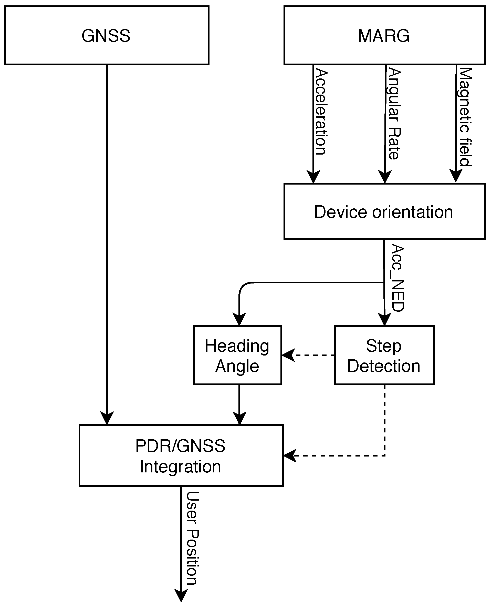
Figure 1 illustrates the block diagram that highlights the operation of the proposed system:
The data coming from the magnetic, angular rate, gravity (MARG) sensor, which is composed of a triaxial accelerometer, gyroscope and magnetometer, is processed by a suitable Madgwick filter in order to obtain the orientation of the mobile device in a fixed North-East-Down (NED) frame; then, the acceleration in NED frame is exploited to identify the single steps, which are used as a trigger signal to drive an algorithm for the estimation of the heading angle of the walk; finally, the data coming from the GNSS is integrated with MEMS data in order to determine the user position. The algorithm for the heading estimation is event-driven, in fact it is essential to identify every single step for determining the direction of advancement of the user’s motion.
In Section 2 materials and methods used to obtain the proposed GNSS/PDR navigation system are illustrated; in particular, the treatment of the methods has been divided into the determination of the device orientation (Section 2.2.1), the step detection (Section 2.2.2), the determination of the motion direction (Section 2.2.3), the step length estimation (Section 2.2.5) and the GNSS/PDR integration (Section 2.2.6). Section 3 describes and discusses the results obtained; finally, Section 4 shows the conclusion of the presented work.
2. Materials and Methods
This section will describe the hardware and methods which are used to achieve the set goals.
2.1. Materials
Mobile devices such as smartphones can differ on technical characteristics including computational power, storage capacity, and available sensors. In this work, a Realme 5 Pro model has been chosen as a mid-range smartphone in order to guarantee the functioning of the implemented system on as many devices as possible. All main technical characteristics of this device are shown in Table 1.
The IMU used in this model of smartphone is the BMI160 [5] produced by Bosch. It has been designed for low power, high precision 6-axis applications in mobile phones, tablets, wearable devices, remote controls, game controllers, head-mounted devices and toys. When accelerometer and gyroscope are in full operation mode, power consumption is typically 925 A, enabling always-on applications in battery driven devices. In this case is a 6-DOF IMU that includes a triaxial accelerometer and gyroscope. Another 3 DOFs are implemented by the triaxial magnetometer that is the AK09918 [6] composed by a triaxial electronic compass IC with high sensitive Hall sensor technology. The Snapdragon 712 chipset of the Realme 5 Pro smartphone allows the access to the following satellite constellations: GPS, GLONASS, BEIDOU, GALILEO, QZSS, and the SBAS. In particular, the GPS, GLONASS, BEIDOU, and GALILEO constellations refer respectively to the American, Russian, Chinese and European global navigation satellite systems; QZSS refers to a regional navigation satellite system aiming to enhance GPS in the Asia-Oceania regions; SBAS refers to the satellite-based augmentation systems aiming to improve the accuracy and the reliability of the GNSS information [7].
An objective of the algorithm that integrates PDR and GNSS is to take rid of the non-stop use of satellite data in order to achieve energy saving. Therefore, it is necessary to choose an appropriate time interval between subsequent activations of the GNSS receiver. In order to obtain comparable data, it was decided to acquire the GNSS data (latitude, longitude, and accuracy associated to the position solution) on a continuous time basis and to implement a control logic to use the data in the algorithm at regular predetermined intervals with a predefined duty cycle. In this way, it was possible to run the GNSS/PDR algorithm multiple times on the same data in order to define the best time interval between subsequent activations of the GNSS receiver. It is necessary to consider that once the satellite receiver is switched on, it will be necessary to wait for a certain time interval to achieve the time to first fix (TTFF), which is a measure of the time required for a GNSS navigation device to acquire the satellite signals, decoding the navigation data, and to calculate a position solution. When smartphones are connected to the mobile network, the TTFF can be either more than a minute or less than a second depending on the type of assistance provided by the mobile network [8]. The system proposed for the integration between GNSS and PDR is suitable for a real time implementation; therefore, it was chosen to implement all the algorithms on Simulink visual programming of the Mathworks development environment.
Figure 2 shows the Simulink diagram of the proposed GNSS/PDR system which assumes the GNSS data available at the initial time of the walk. The data generated by the accelerometer, gyroscope and magnetometer sensors are acquired at a sample rate of 100 Hz. This diagram illustrates the principal system blocks, from the data acquired by the sensors to the information provided as output:
- latitude and Longitude computed by the PDR only;
- latitude and Longitude computed by the GNSS/PDR integration;
- step counted by PLL;
- distance evaluated by the GNSS/PDR integration.
Simulink has been chosen to test the developed algorithms and furthermore, the use of Stateflow has allowed to create blocks that evolve with an event driven logic and therefore are disconnected from the sampling time of the system scheme.
The KF developed for the GNSS/PDR integration considers a state in which the estimated position refers to a North-East local reference frame and represents the distance in meters from the starting point, i.e., the origin of the North-East plane itself. On the other hand, the GNSS readings are originally expressed in latitude and longitude and do not directly provide information consistent with those adopted in the definition of the state variables. A routine, that given two consecutive GNSS readings provides their distance in meters and the angle with respect to the North, is needed to determine the direction of the motion occurred.
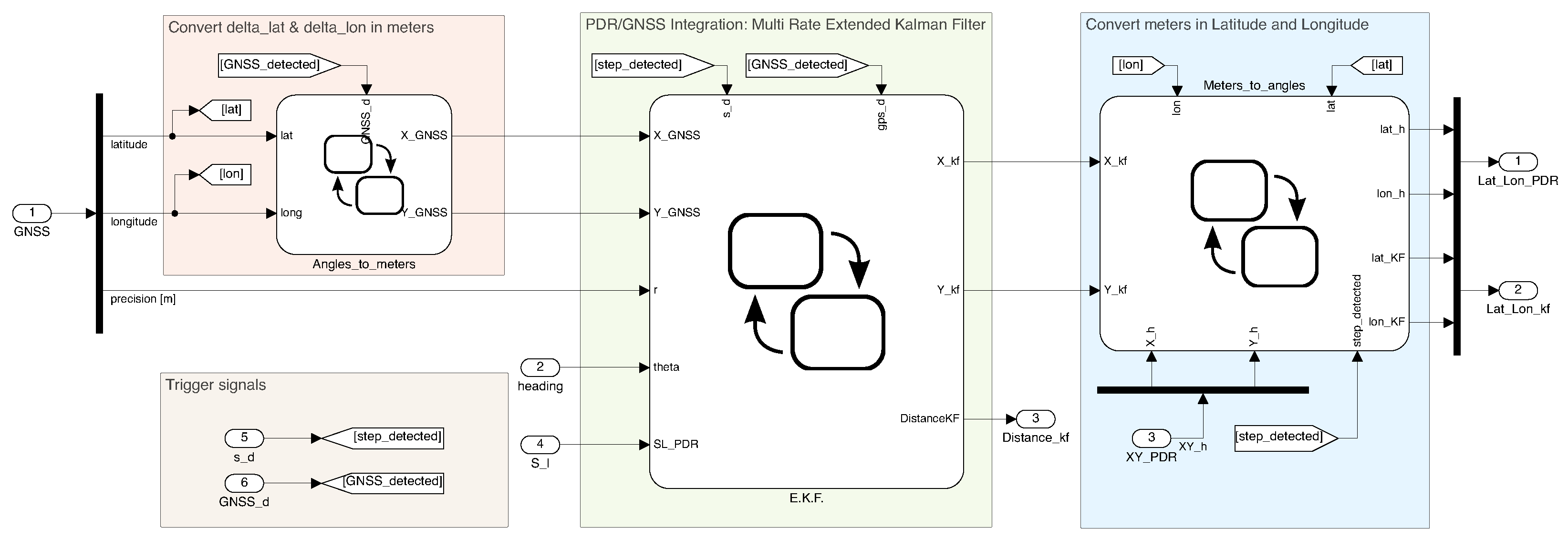
This conversion is carried out by applying the Haversine formula [9] and it has been implemented in Simulink following the diagram in Figure 3, where the GNSS_detectedsignal indicates the presence or absence of satellite data. An Android software application for smartphone has been created to emulate the Simulink schemes through the Simulink Support for Android devices.
The developed GNSS/PDR navigation system works with information coming from the low-cost MEMS sensors mounted on smartphone and its implementation as a state machine allows to execute the calculations necessary for the correct operation between one step and another, creating a control logic with a not excessive computational cost able to be managed by the processor of mobile devices.
2.2. Methods
To develop the proposed pedestrian navigation system (PNS) the following steps are needed:
- realizing an attitude and heading reference system (AHRS) that relies on the data of the inertial sensors;
- identifying each step performed by the user as accurately as possible;
- estimating the step length;
- defining the algorithm for estimating the direction of motion;
- integrating the data from inertial sensors with the global navigation satellite system.
In the following sections, each of these points will be examined in depth in order to provide a clear understanding of the used methods.
2.2.1. Sensor Fusion for Device Orientation Estimation
As it is known, each inertial and magnetic sensor measures a specific physical quantity, but can also be used to derive other information such as the ones related to velocity, orientation, position. Due to the errors that are always present in the measurement, the sensor’s information has to be manipulated (e.g., direct integration of the accelerometer data to estimate the velocity) and the cumulative error on the derived information grows with time. A technique that is used to obtain a more accurate information from the one which is obtained by sensors is the fusion. The aim of the sensor fusion technique for the orientation estimation is to obtain a combined information and to define a stable AHRS. The latter allows to represent the sensor data, originally expressed in the sensor body frame, in a reference frame which permits to represent the sensor orientation on the Earth surface, namely the North-East-Down (NED) frame for this work. The operating systems of Android or iOS devices commonly provide information on the orientation as a function of the Euler angles. In this paper, representing the orientation via unitary quaternion was preferred to Euler angles in order to avoid the gimbal lock problem. When dealing with Euler angles, the gimbal lock phenomenon occurs when one of the sensor axes, used to estimate the angles, aligns with the gravity vector causing a loss of information; this scenario can easily occur when the phone is in the pocket. As a result a Madgwick filter was then implemented to merge the accelerometer, gyroscope and magnetometer data. This filter, reported first time in 2010 by Sebastian O.H. Madgwick [10], represents an efficient way to fuse data for estimating the orientation with respect to a reference fixed navigation frame <e> using quaternion representation. It uses a gradient-descent algorithm to compute the direction of the gyroscope measurement error as a quaternion derivative [11]. The main idea behind the Madgwick filter is to evaluate the orientation from the angular velocity of the gyroscope and correct the resulting bias by evaluating the orientation from homogeneous fields, such as Earth magnetic and gravitational fields, and finally perform a compensation of magnetic distortion.
It is possible to consider the quaternion representation for the rate of change of the Earth frame relative to the sensor frame as
where the accent denotes a normalized vector of the unit length, is the quaternion representation of the angular rate elements at time t from gyroscope expressed in referred to sensor frame, and the symbol ⊗ represents the quaternion product that can be determined using the Hamilton rule:
The quaternion that expresses the orientation of the Earth frame relative to the sensor frame considering only the gyroscope data can be calculated through direct integration as follows:
where is the sample time.
It is necessary to obtain the orientation from the accelerometer and the magnetometer to compensate for the errors that are made in the integration of the gyro bias. The attitude estimation from the accelerometer or magnetometer is done by using a gradient descent algorithm to solve the following minimization problem. The orientation of the sensor frame, , is that which aligns a predefined reference direction of the field in the Earth’s frame, , with the measured direction of the field in the sensor frame , using the rotation operation
2.2.2. Step Detection
In order to perform an effective pedestrian dead reckoning algorithm, the design of a procedure capable of determining the occurrence of each step performed by the user becomes crucial. The step identification from the acquired inertial data can be achieved by means of various techniques that are referred in the literature, including the identification of peaks on the acceleration signal, the use of phase-locked loop (PLL) systems to build a signal that is easier to analyze [13], or the use of wavelet transform to detect the step boundaries over time [14,15]. All these systems are based on a preliminary gait analysis: in fact the signals coming from the inertial sensors strongly depend on the area of body in which the device is worn and its relative orientation between this part and the direction of motion. The study done in Section 2.2.1 allows us not to worry about the orientation as it is possible to bring the data from the sensor body frame to a reference fixed one, so permitting to consider only the area of the body where the device is worn. In this work, the device is considered worn in the pocket of the user who is assumed to perform a walking activity or to remain stationary. Particular actions or movements such as jumping, sitting down or standing up are not taken into consideration in this work.
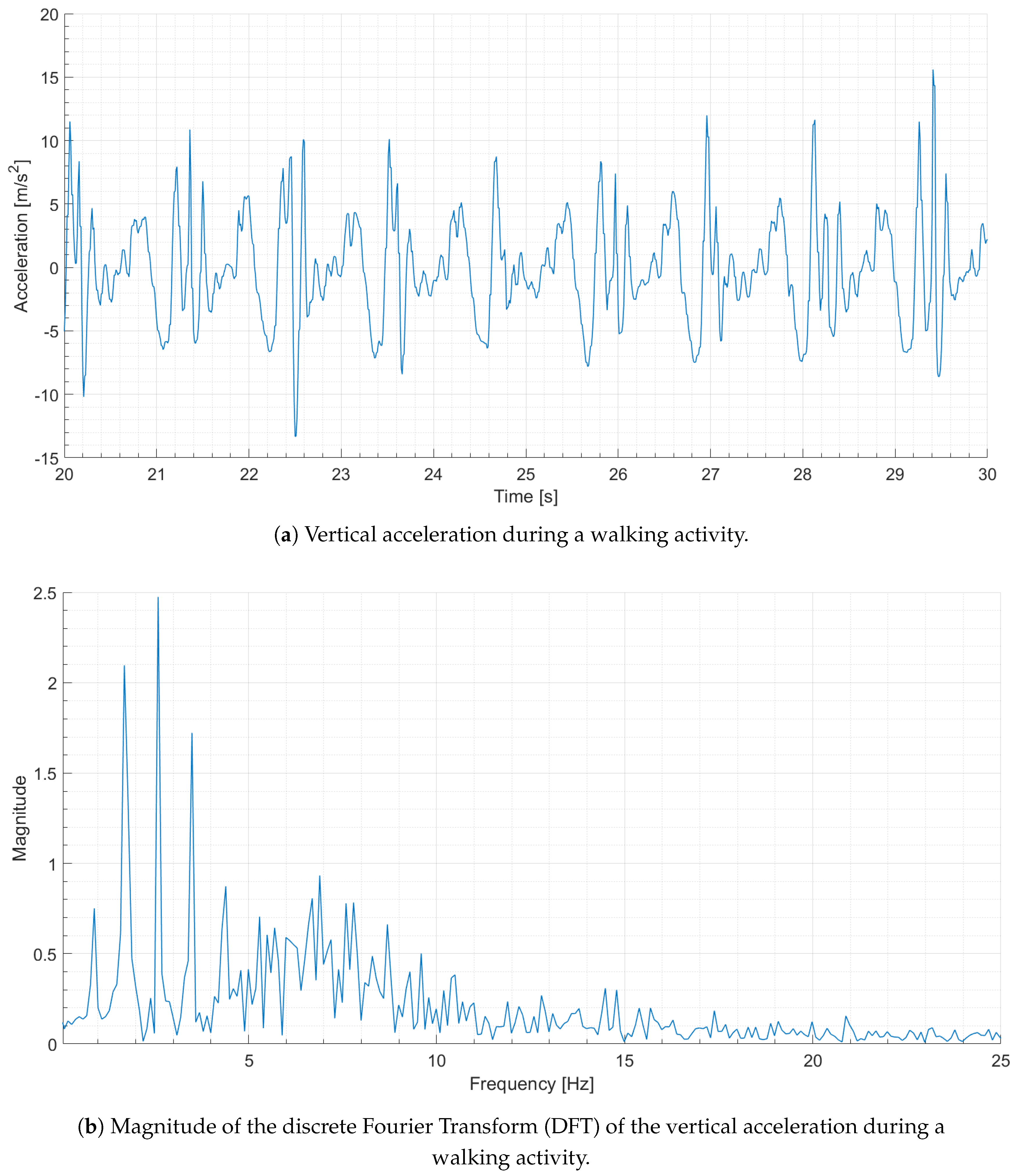
A discrete Fourier transform (DFT) analysis has been performed off-line on the available data referred to the vertical acceleration in NED frame. The aim of this evaluation is to indicate where the dominant frequencies associated to the step frequency can lie in the frequency domain. The results show a main harmonic component at 1.8 Hz which is used by the system in the real-time implementation to initialize the free running frequency of the PLL. In addition to the main harmonic component, the vertical acceleration presents higher frequency content for several reasons: the oscillatory motion of the pelvis, the vibration due to a device not rigidly attached to the body, and the noise. In order to highlight the main harmonic component associated to the step frequency, the vertical acceleration in the NED frame has been pre-processed through a low-pass filtering operation. A Chebyshev low-pass infinite impulse response (IIR) filter with a cut-off frequency of 15 Hz has been used. Since the group delay of the IIR filer is not constant, the latency introduced by the filtering depends on the frequency of the input signal; for what concerns the input signal considered in this work, the mean latency is about 0.4 s. The cut-off frequency of 15 Hz has been chosen because the principal information content in the frequency domain of the acquired vertical acceleration signal lies on the 0–15 Hz interval, as shown in Figure 4. Therefore, the frequency content above 15 Hz has been considered as a noise signal.
The main harmonic component of the signal represents the step frequency and each maximum acceleration peak identifies the step event. A suitable PLL has been developed in order to create a sinusoidal signal which is locked in phase to the vertical acceleration signal with a free running frequency close to that considered valid for walking, i.e., equal to 1.8 Hz.
Figure 5 compares the vertical acceleration in the NED frame and the sinusoidal signal that is the output of the PLL. The latter simplifies the identification of the steps occurred by coupling them with the relative maxima in a real-time implementation. In order to avoid that the PLL locks onto signals that are not related to walking, it is useful to implement a logic circuitry that automatically recognizes the carried out activity. Therefore, the variance of the vertical acceleration in the NED frame has been considered to evaluate the motion intensity of the user. In particular, the variance analysis has been performed over a 4-s moving window and the threshold of 1.5 m2/s4 has been empirically determined to distinguish the motion activity from the stationary case.
2.2.3. Heading Estimation
The heading angle is defined as the angle between the North direction and the motion direction of the person wearing the device. Estimating the motion direction is the most critical part of a pedestrian inertial navigation system due to the complexity of the body motion and the degrees of freedom of the human body. In fact, the walking motion, that can theoretically change at every single step, is not predictable. There are several ways to deal with this problem; for example, it is possible to fix the position of the inertial sensors in a rigid way at chest level or in a belt in order to be able to have a preferential direction of motion [14,15]. This drastically reduces the degrees of freedom of the system, but represents a situation that cannot be reproduced in a common scenario, in fact a phone is normally kept in a pocket or held in the hand during a walk or in an armband for running. For this reason, a system that is independent of the choice of the device location on body is needed. The considered method, which will be described below, exploits the fact that the acceleration data reported in NED frame can be used to determine the direction of motion. Considering the phone worn on the upper part of the leg, then the acceleration values in the North and East directions are related to the direction of motion and can be used to determine the heading angle. As reported in [13], by analyzing the accelerations on the North and East axes in the NED frame ( and ) at each couples of steps, it is possible to identify pseudo-ellipses, as shown in Figure 6.
Even if the shape of the double ellipse is not exactly reproduced at each pair of steps, it is still possible to determine the direction of the motion quite clearly within a tip-to-tail method, except in the case of irregular steps. This method is based on the direct use of the filtered acceleration data. Despite the implementation of the filter, it is possible that the signal is distorted by harmonics higher than that relating to the dynamics of the steps. The idea behind the real-time implementation of this method is to find a direct formula that can provide the heading angle starting from the Fourier series decomposition of the input planar acceleration signal. It is well known from theory that any periodic signal can be decomposed into the sum of an infinite set of simple oscillating functions, namely sines and cosines. Though the walking signal is not periodic, however, if the period of the single step and consequently its frequency can be determined with some accuracy, it is possible to consider a periodic extension of this signal on which applying the Fourier series decomposition that is valid only in the considered step period. An accurate step tracking system using a PLL to analyze acceleration data can relate the steps taken with the stride characteristics, thereby providing a trigger signal for the forward direction estimation algorithm.
The Fourier series at each single step detect is defined as:
where the subscript k identifies the number of the step occurred, is the period of the last detected step that can be calculated as the time between the start of the step () and its end, that is also the start of the next step ():
and are the so called Fourier coefficients that are computed as follows:
where n is the number of harmonics considered for the approximation. With this method the direction estimate takes place considering only the time interval of the last step and not of the last two as for the previously described method. Let be the planar acceleration vector
and considering the first harmonic of the corresponding Fourier series
where
It can be shown that Equation (10) represents an ellipse centered at the origin whose principle axis is rotated by a certain angle. Indeed, it is possible to rewrite (10) as
where the four values of integrals described in (8) become
Now the objective is to find a relationship between the four values of the integrals and the inclination angle of the rotated ellipse that represents the direction of motion. This problem can be solved under the following assumption (1st order approximation):
Referring to Figure 7, the goal is to find the point , where To this aim, the square of the 2-norm of the planar acceleration can be approximated as
Finally, assuming
and exploiting common trigonometric formulas yields
In order to find the time corresponding to the maximal value of the planar acceleration, it is necessary to set to zero the derivative with respect to time
which yields
By substituting the actual values of , A, B it is possible to write as a function of the four integrals
where the correct solution is the first one providing a negative second order derivative
Finally, considering the point , the heading angle in the NED frame results in
By averaging two consecutive values of the heading angle, it is possible to obtain a smoothed signal for which the occurring spikes or errors given by the pelvis rotation during walking are reduced.
2.2.4. Summary of the Heading Estimation Algorithm
In summary, the algorithm for determining the heading angle in real time has the following structure:
- acquire the planar acceleration data in NED frame: , ;
- exploit an available step identification system, such as the one provided by the PLL, that provides the time between each single step ;
- for each step detected :
- (a)
- compute the Fourier coefficients () from which it is possible to calculate
- (b)
- calculate :
- (c)
- if update adding a quarter of period: ( function will give nearest solution);
- (d)
- check that the second derivative of the acceleration module calculated in is less than zero to be sure that refers to a maximum point; otherwise update adding a quarter of period: ;
- (e)
- compute the heading angle :
Remark 1.
Notice that the values of the integrals (13), that correspond to the Fourier coefficients, assume a valid meaning only at the end of each step, but nonetheless need the information relating to the time taken to carry out the step to compute sine and cosine functions. For this reason, it was decided to provide the time elapsed on the last step to estimate the Fourier coefficients at the current step. This approximation does not dramatically affect the heading angle estimation due to the regularity of the step frequency.
Remark 2.
This heading calculation does not take into account the difference between magnetic north and true north (the direction along a meridian towards the geographic North Pole). This difference is called magnetic declination and varies depending on the position on the Earth surface and changes over time. By convention, declination is positive when magnetic north is east of true north, and negative when it is to the west. The magnetic declination in a given area may change slowly over time, possibly as little as 2–2.5 degrees every hundred years, so it could be considered constant for this implementation. A good implementation requires an evaluation of the declination angle when the application starts in order to achieve information about the place where the smartphone is. A website like https://www.magnetic-declination.com (access date: 15 December 2021) can provide this information, in Florence, Italy the declination is degrees.
2.2.5. Step Length Estimation
In the PDR navigation, the step length estimation presents a high number of variables: in particular, the measurements of the inertial sensors are influenced by the location where the device is worn and the stride length strongly depends on the physical characteristics of the user and the type of motion that is performed. In literature, it is possible to find mathematical models that relate the length of the steps with frequency and height of the user [16].
The length of the k-th step can therefore be expressed as a function of the frequency of the step as follows:
where a and b are parameters that depend on the physical characteristics of the user. Furthermore, it must be considered that during a walk some steps can be irregular and in some situations it is necessary to avoid obstacles, stopping or changing direction. All these elements increase the uncertainty on the estimation of the step length. For these reasons, it seems reasonable to determine the step length as a mean of multiple step lengths. By dividing the steps performed over the distance traveled between two successive readings of position from the satellite navigation system, it is possible to obtain the average length of the step. By means of the average step length value given by the method that uses the satellite readings, it is possible to correct any offset of the mathematical model previously described. To avoid that the estimation of the step length strongly depends on the physical characteristics of the user, a strategy that dynamically modifies the parameters of the model (23) can be implemented, or additionally can provide compensation of systematic errors from the information of the satellite data [17].
2.2.6. GNSS/PDR Integration
By estimating the step length and the heading angle, it is possible to determine the user’s trajectory by using pedestrian dead reckoning techniques, where the information of step length () and heading angle () is available each time a new step is detected [18,19]. Let and the position of the device in the reference system at k-th step detected, the PDR technique expresses its evolution as
In this algorithm, it is evident that the estimation of the step length plays a fundamental role: small errors on this parameter, being added step by step, can lead to large errors in the reconstruction of the path on the map. On the other hand, errors on the heading angle, as expected, can lead to a deviation from the true path.
The PDR technique alone is not able to perform an absolute positioning of the device, and therefore must necessarily be integrated with a satellite navigation system. A global navigation satellite system (GNSS) can be used to integrate a PDR and correct errors that accumulate over time, but nevertheless it causes a high energy consumption in mobile devices and the accuracy of its readings are highly dependent on the operational context as it is based on the use of an infrastructure, i.e., how many satellites are visible in the constellation and the quality of the received signals. For these reasons, it is useful to implement a filter that merges the data coming from the inertial sensors with the satellite ones, as shown in detail in [17]. The proposed Kalman filter (KF) does not evolve at each sampling time, but that is executed following a trigger event, which in this case is provided by the procedure of the step detection. It is also right to underline the fact that the signals coming from the PDR and GNSS are generally asynchronous, in fact the PDR processes information at each step detected, while the GNSS data can usually update at 4 Hz as maximum frequency and as mentioned will not always be available. With an extrapolation technique it is possible associate last valid data from GNSS measurement with last step occurred. In this application, a GNSS signal is constantly acquired and a signal that gives information about its validity is associated to. To correctly implement the KF, a signal that triggers the failure of the GNSS is necessary. There are two different solutions to implement the lost of signal and both refers to a multi-rate KF:
- covariance-varying approach: when no GNSS signals are available, it can be modeled as a sensor with a high covariance matrix related on its measure, so by varying the covariance the KF will not consider the readings in its update [20];
- size-varying approach: when no GNSS signals are available, it can be modeled as a changing of the number sensor used for measurement and as consequence the dimension of measurement equations and its covariance matrix will change [21].
A size-varying approach was chosen in order to implement two different strategies:
- best performance algorithm: the KF continuously uses the satellite data, when present, by correcting the positioning errors deriving from the estimate that is made using only inertial data;
- energy-saving algorithm: the KF uses the satellite data at regular time intervals in order to allow the satellite receiver to be switched off.
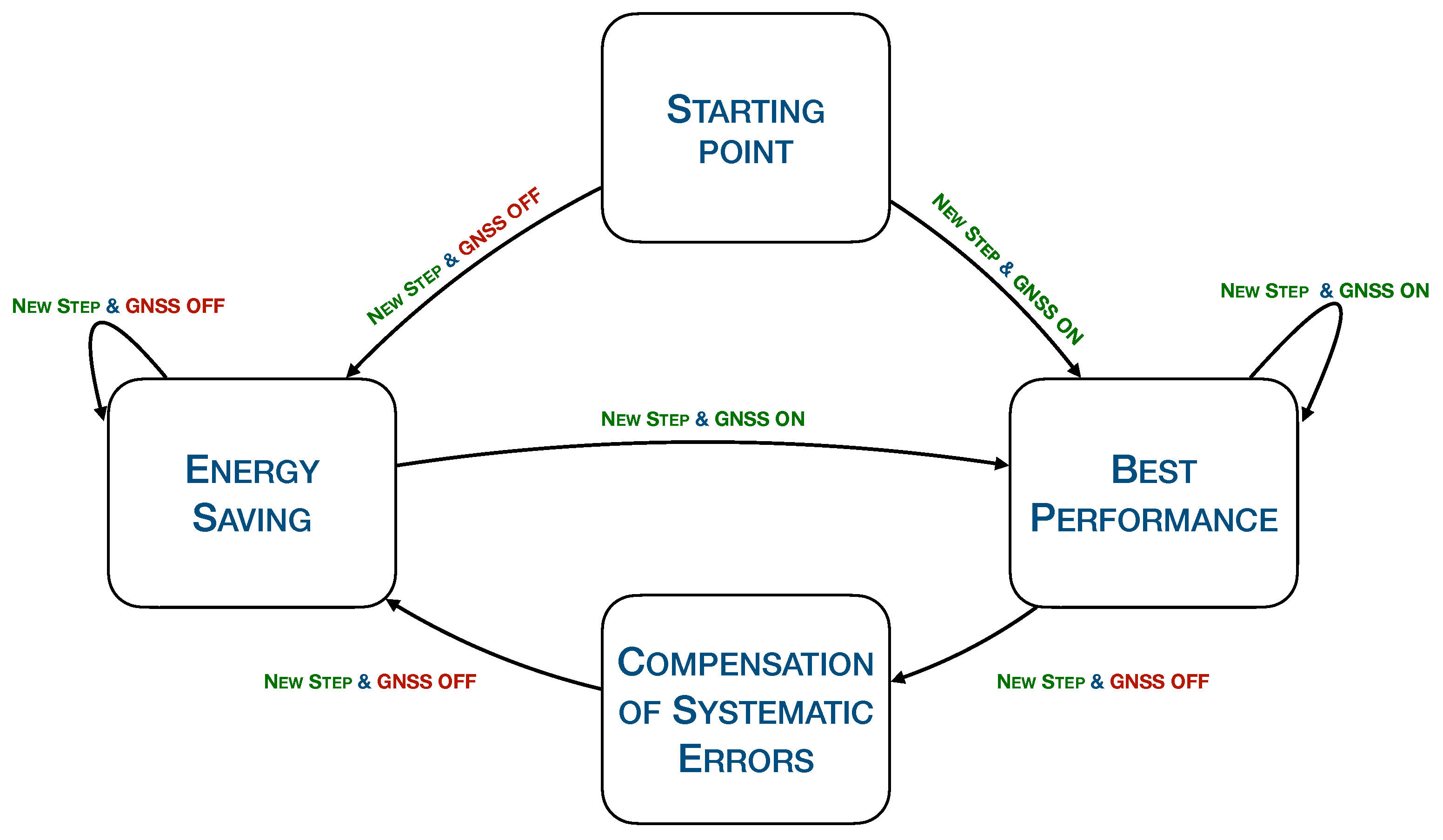
Thus, the designed structure of the filter can be seen as a state machine that evolves every time a new step is detected and has a different behavior depending on the presence or not of the satellite data. Furthermore, between one restart and the subsequent one of the GNSS, it is possible to implement a compensation strategy of the systematic errors that are committed on the determination of the estimate of the step length and the heading angle [17]. Figure 8 shows a block diagram of the operating principle of the described filter.
3. Results
In this Section, the experimental results of the the proposed GNSS/PDR system are described and discussed.
3.1. GNSS/PDR Integration
In this Section, the experimental results of the algorithm both in the best performance and in the power saving modes will be shown. The position results that have been obtained by using only inertial data, and therefore using the PDR method, will be compared with those obtained from GNSS data and the reconstruction of the KF.
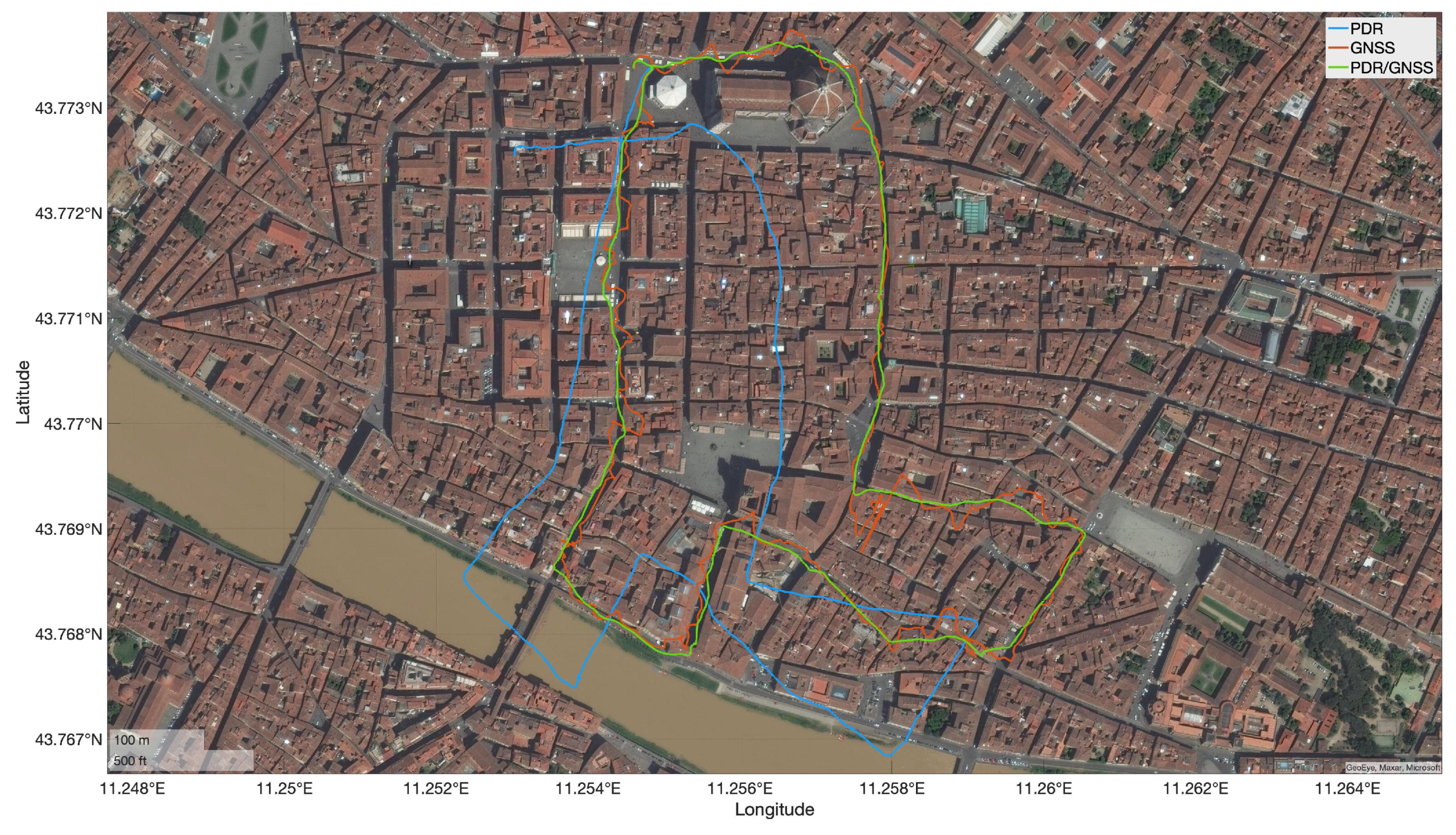
In all the figures in this paragraph, the blue line represents the path which is obtained by INS using the DR technique; the orange line represents the interpolation of the GNSS readings, which have been left continuously active in order to choose different GNSS update interval to be adopted in the energy saving routines; the green line represents the path reconstructed by the KF with appropriate corrections of systematic errors in the case of energy saving. The carried out tests have been performed by walking at an average pace in an urban environment, so emulating a typical everyday situation. The urban environment is in fact a typical scenario in which there may be disturbances on the Earth magnetic field given by vehicles and buildings. Tall buildings can decrease the accuracy of the GNSS data and a path that is not free from obstacles does not guarantee the stability of the direction of motion and the regularity of the steps. These difficulties represent an excellent scenario on which to test the developed algorithm.
3.1.1. Best Performance
In the best performance case, the GNSS signal is continuously detected and therefore for each detected step the KF updates the state estimate by merging the inertial data with the last GNSS reading. It is important to note that the GNSS chipset, in addition to the position solution expressed in latitude and longitude values, provides a value that represents the accuracy associated to the position and therefore the reliability of the data at that instant of time. In this way, the KF gives more or less importance to the value read from the GNSS.
Figure 9 shows the results for this case. It is possible to notice how the path that is reconstructed only from the inertial data (blue line) deviates from the others due to the accumulation of errors, as foreseen by the PDR method. The position results related to GNSS data, on the other hand, is strongly influenced by the accuracy with which the position solutions are determined and being an urban route it is not always sufficiently high.
It is also possible to note that the signal reconstructed by the KF inherits the advantages of both methods: the smoothness of the PDR navigation and the bounded position error provided by the GNSS. In the area where the satellite signal has poor accuracy, the filter properly weights the GNSS information without following the latitude and longitude readings.
On the other hand Figure 10 shows the GNSS position accuracy along the test: the average value is less than 50 m, but in some conditions the accuracy can rise up to 250 m, making the relative latitude and longitude readings useless.
3.1.2. Energy Saving
In the energy saving mode, a parameter related to the frequency with which the GNSS data is queried has to be chosen. In fact, it is necessary to choose how often to turn on the GNSS reading system to use this information, once it is considered valid. The longer this interval, the greater the energy savings and the error introduced by the PDR [17]. It is worth noting that in the power saving mode there is the functionality for the correction of systematic errors. This correction is carried out when the GNSS signal is turned off on the basis of the last information considered valid for the position; it is done in real time and applied to subsequent data. In this way, the position estimated by the KF for the subsequent data takes into account the errors previously occurred; these errors can be corrected in the previous trajectory by carrying out a similar correction, but on the past estimates.
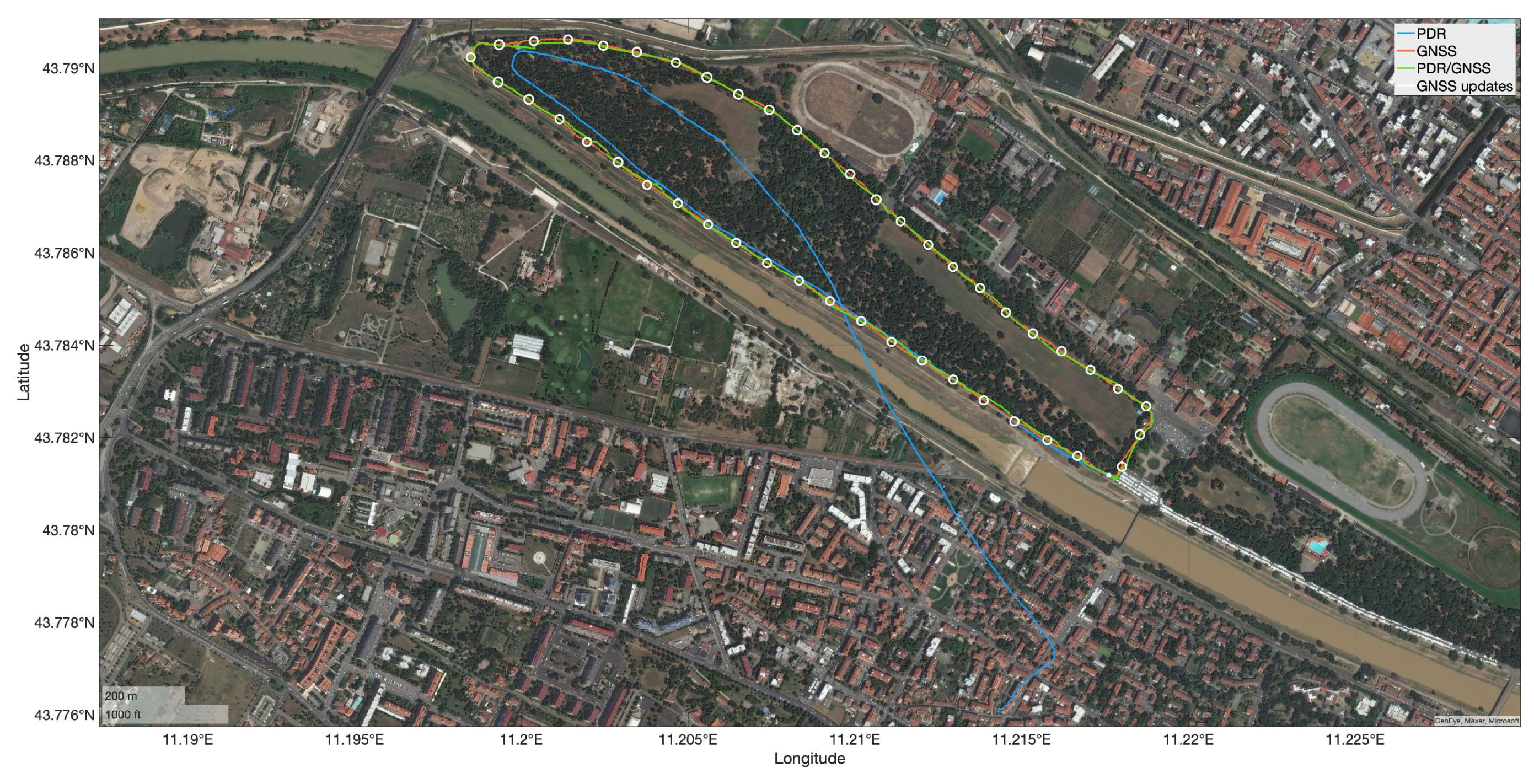
In the following figures, the white circles highlight the corrections that have been applied to the GNSS readings at pre-established time intervals. These circles are centered in the corresponding GNSS reading and the range depends on the relative accuracy of that reading. Therefore, the KF correction will be more evident where the radius of the circle is smaller.
Figure 11 shows the results if a time interval between two consecutive GNSS readings of 60 s is chosen. This time interval was chosen as a suitable trade-off between the energy saving and the reconstruction quality of the trajectory.
In fact, by increasing the duration of the time interval between two successive readings of the GNSS data, for example by bringing it to 180 s as shown in Figure 12, it is possible to highlight the errors due to the fact that the path between two readings are compensated with the information of corrections evaluated in the previous interval and not in the current one. However, it is possible to use the proposed method as a real-time positioning system and leave the task of reconstructing the path to another algorithm as proposed by [17]. It is important to highlight that the energy saving amount is totally dependent on the smartphone model, the simulation setting and the test environment, which means these values cannot be generalized for common systems. Nonetheless the impact of the energy saving routine can be estimated on a relative basis taking into account the time needed for a valid GNSS fix (in “hot start” condition). Indeed, once the GPS fixing has been performed, this unit is switched off and the longer is the switch off interval, the higher the energy saving. This consideration is based on referred results [17].
Figure 13 highlights the behavior of the algorithm in a context where the satellite signal present an accuracy less then 12 m. Also in this case the update interval between one reading and the next of the satellite data has been set to 60 s and the readings result reliable and therefore always useful for the correction of systematic errors.
4. Conclusions
This article provides an overview of the design and the development of a pedestrian navigation systems using information from different sensors present in smartphones. In particular, it has been highlighted the importance of an accurate technique to determine the individual steps and how crucial a proper implementation of a PLL can be for this goal. To determine the direction of motion at each detected step, an algorithm that evaluates the second harmonic component of the planar acceleration has been developed. From the knowledge of this signal, through analytical and geometric considerations, the direction of motion was calculated using a closed-form mathematical solution. This innovative approach allows to calculate the direction of motion in real time and to use this information in a dead reckoning method for estimating the current position with respect to a North-East local reference frame. It is important to underline that this system has been designed to work with the mobile device in a pocket, being independent of its orientation during the motion activity.
Moreover, a Kalman Filter for the integration of a pedestrian dead reckoning navigation system with a global navigation satellite system has been developed. A multi-rate filter was developed according to the size varying approach as the satellite system information is not always available. Finally, the algorithm provides the positioning values in real time by updating the latitude and longitude angles in order to show the current estimated position on the map. In order to validate the performance of the system, tests were carried out both in an urban environment, where the accuracy of the GNSS is lost due to the passage between tall buildings, and in an open environment where the visibility of the satellite is clear. Where the GNSS accuracy is high, the best performance filter that continuously uses the GNSS data has the best results, whereas in several situations where the GNSS signal is particularly degraded, the energy saving filter with an appropriate update interval brings some advantages.
Our current activity is aimed at estimating the saved energy amounts and the update interval: to this aim different time intervals are taken into account by analyzing the battery drain and the energy impact of the processor when processing the GNSS/PDR algorithm. These results will be dealt with in future publications.
Author Contributions
Conceptualization, M.B., A.M., S.M. and F.S.; methodology, M.B., A.M., S.M. and F.S.; software, M.B., A.M., S.M. and F.S.; validation, M.B., A.M., S.M. and F.S.; formal analysis, M.B., A.M., S.M. and F.S.; investigation, M.B., A.M., S.M. and F.S.; resources, M.B, A.M., S.M. and F.S.; data curation, M.B., A.M., S.M. and F.S.; writing—original draft preparation, M.B., A.M., S.M. and F.S.; writing—review and editing, M.B., A.M., S.M. and F.S.; visualization, M.B., A.M., S.M. and F.S.; supervision, M.B., A.M., S.M. and F.S.; project administration, M.B., A.M., S.M. and F.S. All authors have read and agreed to the published version of the manuscript.
Funding
This research received no external funding.
Informed Consent Statement
Not applicable.
Data Availability Statement
Not applicable.
Conflicts of Interest
The authors declare no conflict of interest.
Abbreviations
The following abbreviations are used in this manuscript:
| AHRS | Attitude and Heading Reference System |
| DOF | Degrees Of Freedom |
| DR | Dead Reckoning |
| DFT | Discrete Fourier Transformation |
| GNSS | Global Navigation Satellite System |
| IMU | Inertial Measurement Unit |
| INS | Inertial Navigation System |
| KF | Kalman Filter |
| MARG | Magnetic, Angular Rate, Gravity |
| NED | North East Down |
| PLL | Phase-Locked Loop |
| PDR | Pedestrian Dead Reckoning |
| PNS | Pedestrian Navigation System |
References
- Lamonaca, F.; Polimeni, G.; Barbé, K.; Grimaldi, D. Health parameters monitoring by smartphone for quality of life improvement. Measurement 2015, 73, 82–94. [Google Scholar] [CrossRef]
- Groves, P. Principles of GNSS, Inertial, and Multisensor Integrated Navigation Systems; Artech House: Norwood, MA, USA, 2013. [Google Scholar]
- Angrisano, A.; Vultaggio, M.; Gaglione, S.; Crocetto, N. Pedestrian localization with PDR supplemented by GNSS. In Proceedings of the European Navigation Conference (ENC), Warsaw, Poland, 9–12 April 2019; pp. 1–6. [Google Scholar]
- Giarré, L.; Pascucci, F.; Morosi, S.; Martinelli, A. Improved PDR localization via UWB-anchor based on-line calibration. In Proceedings of the 4th International Forum on Research and Technology for Society and Industry (RTSI), Palermo, Italy, 10–13 September 2018; pp. 1–5. [Google Scholar]
- Sensortec, B. BMI160-Data sheet. Prod. Specif. 2018. Available online: https://www.mouser.com/datasheet/2/783/BST-BMI160-DS000-1509569.pdf (accessed on 11 March 2021).
- Asahi Kasei Microdevices Corporation. AK09918 3-axis Electronic Compass. Prod. Specif 2017. Available online: https://www.akm.com/cn/en/products/electronic-compass/ (accessed on 11 March 2021).
- Hegarty, C.J.; Kaplan, E.D. Understanding GPS/GNSS: Principles and Applications; Artech House: Norwood, MA, USA, 2017. [Google Scholar]
- van Diggelen, F. A-GPS: Assisted GPS, GNSS, and SBAS; Artech House: Norwood, MA, USA, 2009. [Google Scholar]
- Veness, C. Calculate distance, bearing and more between Latitude/Longitude points. In Movable Type Scripts; 2002–2019 MIT Licence; Available online: https://www.movable-type.co.uk/scripts/latlong.html (accessed on 11 March 2021).
- Madgwick, S. An efficient orientation filter for inertial and inertial/magnetic sensor arrays. Rep. x-io Univ. Bristol (UK) 2010, 25, 113–118. [Google Scholar]
- Hasan, M.A.; Rahman, M.H. Smart Phone Based Sensor Fusion by Using Madgwick Filter for 3D Indoor Navigation. Wirel. Pers. Commun. 2020, 113, 2499–2517. [Google Scholar] [CrossRef]
- Al-Fahoum, A.S.; Abadir, M.S. Design of a Modified Madgwick Filter for Quaternion-Based Orientation Estimation Using AHRS. Int. J. Comput. Electr. Eng. 2018, 10, 174–186. [Google Scholar] [CrossRef] [Green Version]
- Basso, M.; Galanti, M.; Innocenti, G.; Miceli, D. Pedestrian dead reckoning based on frequency self-synchronization and body kinematics. IEEE Sens. J. 2016, 17, 534–545. [Google Scholar] [CrossRef]
- Martinelli, A.; Gao, H.; Groves, P.D.; Morosi, S. Probabilistic context-aware step length estimation for pedestrian dead reckoning. IEEE Sens. J. 2017, 18, 1600–1611. [Google Scholar] [CrossRef]
- Martinelli, A.; Morosi, S.; Del Re, E. Daily movement recognition for dead reckoning applications. In Proceedings of the International Conference on Indoor Positioning and Indoor Navigation (IPIN), Banff, AB, Canada, 13–16 October 2015. [Google Scholar]
- Renaudin, V.; Susi, M.; Lachapelle, G. Step length estimation using handheld inertial sensors. Sensors 2012, 12, 8507–8525. [Google Scholar] [CrossRef] [PubMed]
- Basso, M.; Galanti, M.; Innocenti, G.; Miceli, D. Triggered INS/GNSS Data Fusion Algorithms for Enhanced Pedestrian Navigation System. IEEE Sens. J. 2020, 20, 7447–7459. [Google Scholar] [CrossRef]
- Jin, Y.; Toh, H.S.; Soh, W.S.; Wong, W.C. A robust dead-reckoning pedestrian tracking system with low cost sensors. In Proceedings of the 2011 IEEE International Conference on Pervasive Computing and Communications (PerCom), Seattle, WA, USA, 21–25 March 2011; pp. 222–230. [Google Scholar]
- Jirawimut, R.; Ptasinski, P.; Garaj, V.; Cecelja, F.; Balachandran, W. A method for dead reckoning parameter correction in pedestrian navigation system. IEEE Trans. Instrum. Meas. 2003, 52, 209–215. [Google Scholar] [CrossRef]
- Shin, S.; Park, C.; Kim, J.; Hong, H.; Lee, J. Adaptive step length estimation algorithm using low-cost MEMS inertial sensors. In Proceedings of the 2007 IEEE Sensors Applications Symposium, San Diego, CA, USA, 6–8 February 2007; pp. 1–5. [Google Scholar]
- Armesto, L.; Chroust, S.; Vincze, M.; Tornero, J. Multi-rate fusion with vision and inertial sensors. In Proceedings of the IEEE International Conference on Robotics and Automation, ICRA’04, New Orleans, LA, USA, 26 April–1 May 2004; Volume 1, pp. 193–199. [Google Scholar]
Figure 1.
Block diagram of the operating principle of the proposed GNSS/PDR navigation system.

Figure 2.
Simulink diagram of the proposed GNSS/PDR system.

Figure 3.
Simulink diagram of the GNSS/PDR integration.

Figure 4.
Representation in the time and frequency domains of the vertical acceleration during a walking activity. Vertical refers to the down direction of the NED frame.
Figure 4.
Representation in the time and frequency domains of the vertical acceleration during a walking activity. Vertical refers to the down direction of the NED frame.

Figure 5.
The vertical acceleration signal given to the PLL as input (orange line) and the signal provided by the PLL as output (blue line).
Figure 5.
The vertical acceleration signal given to the PLL as input (orange line) and the signal provided by the PLL as output (blue line).
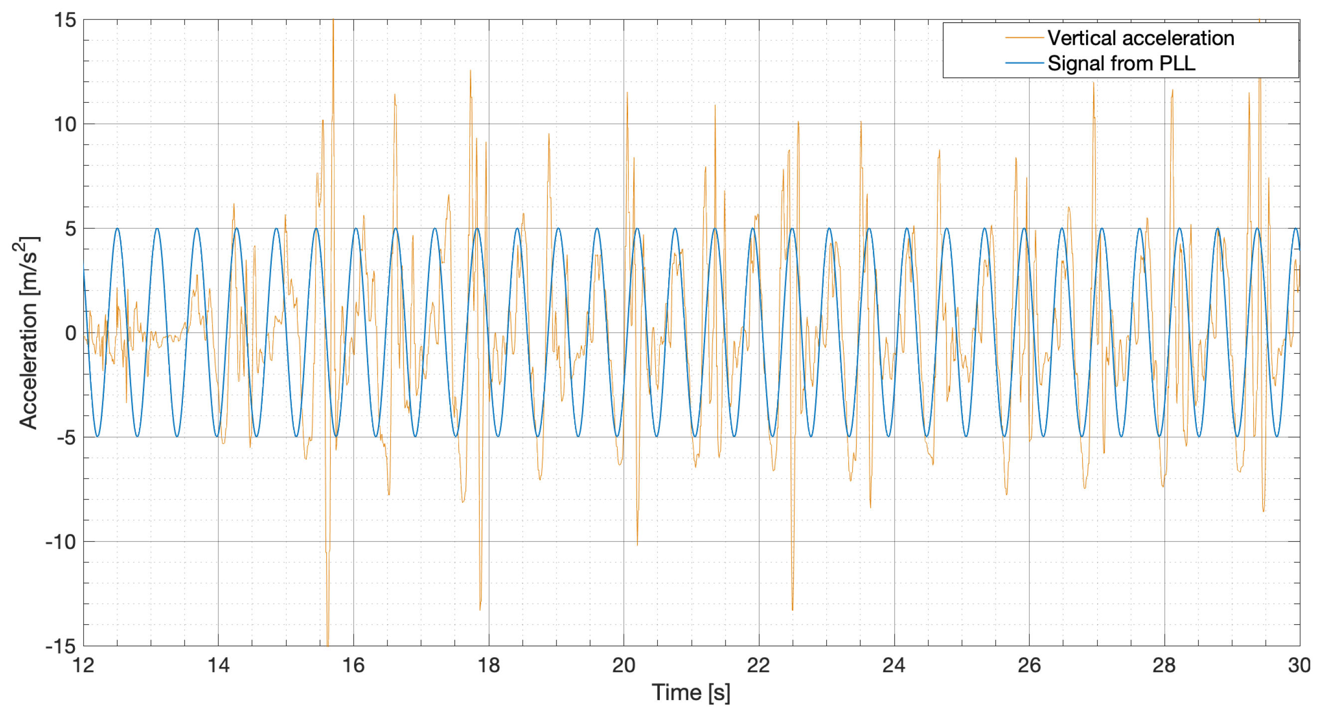
Figure 6.
Representation of filtered and expressed in NED frame on the plane during a sequence of left and right steps.
Figure 6.
Representation of filtered and expressed in NED frame on the plane during a sequence of left and right steps.
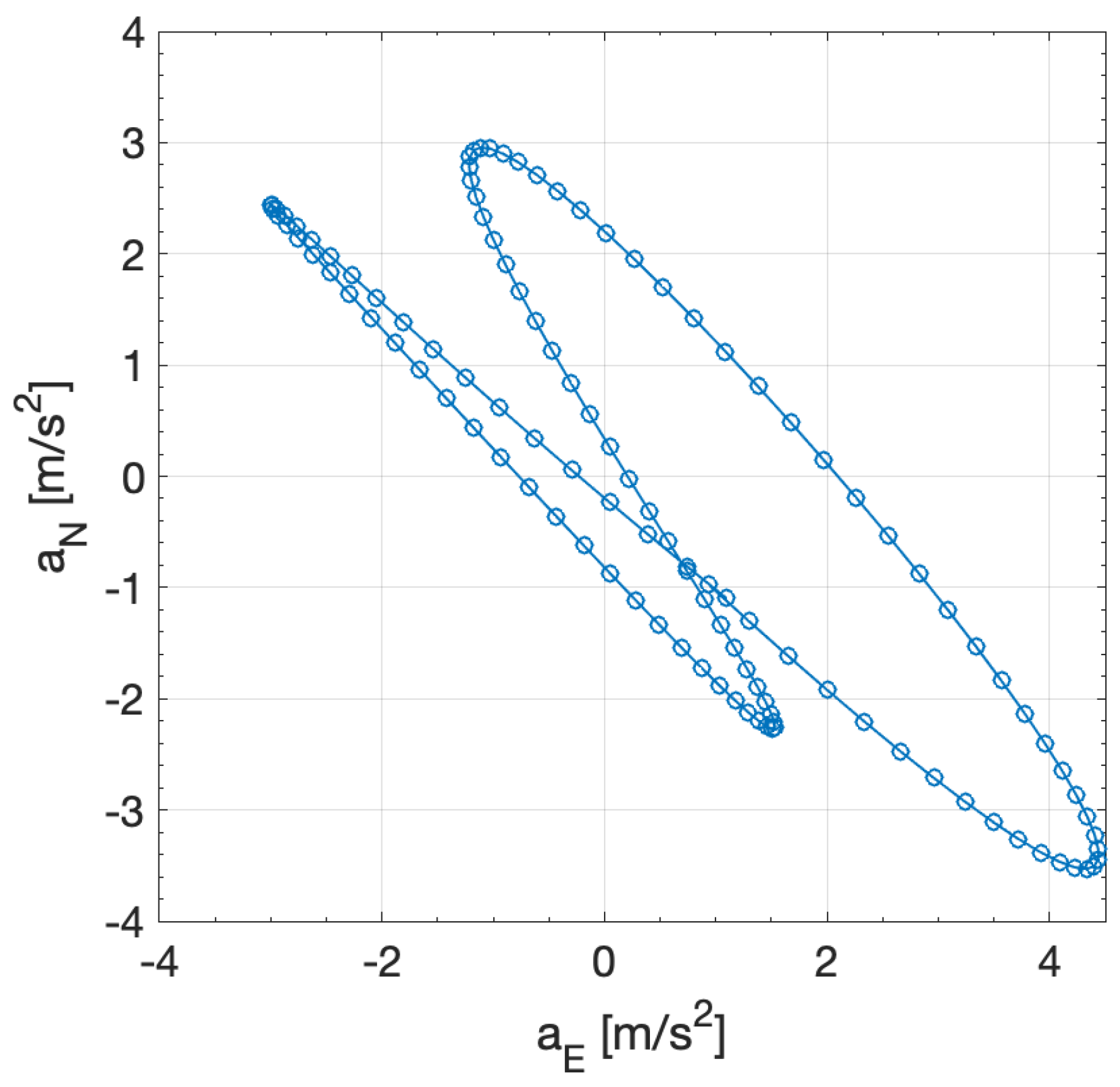
Figure 7.
Rotated ellipse and planar acceleration.

Figure 8.
Scheme of state machine for multi-rate Kalman filter with compensation of systematic errors.
Figure 8.
Scheme of state machine for multi-rate Kalman filter with compensation of systematic errors.

Figure 9.
Comparison between the reconstructions performed by the PDR data, the GNSS data and the best performance fusion algorithm.
Figure 9.
Comparison between the reconstructions performed by the PDR data, the GNSS data and the best performance fusion algorithm.

Figure 10.
Accuracy of the GNSS position solutions computed during a walk in an urban environment.
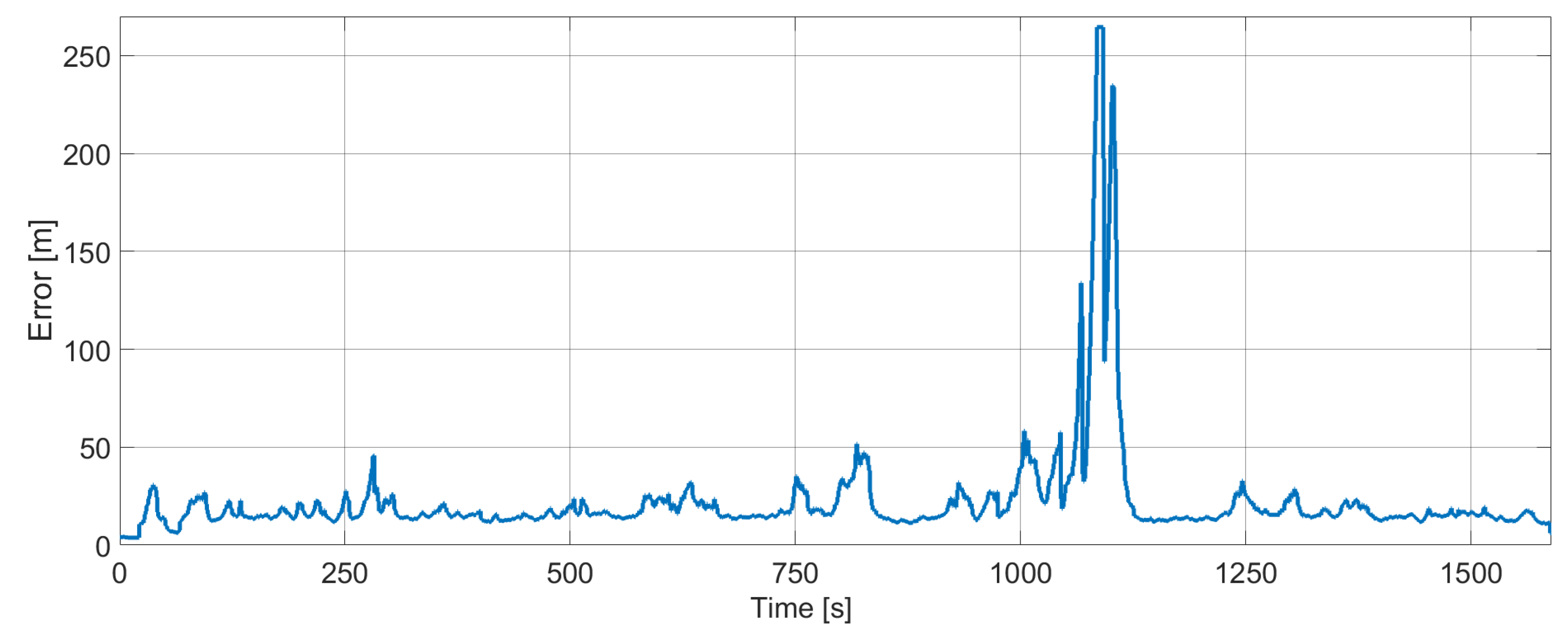
Figure 11.
Comparison between the reconstructions performed by the PDR navigation, the GNSS data and the energy saving fusion algorithm with 60 s as interval between two consecutive GNSS activations in an urban environment.
Figure 11.
Comparison between the reconstructions performed by the PDR navigation, the GNSS data and the energy saving fusion algorithm with 60 s as interval between two consecutive GNSS activations in an urban environment.
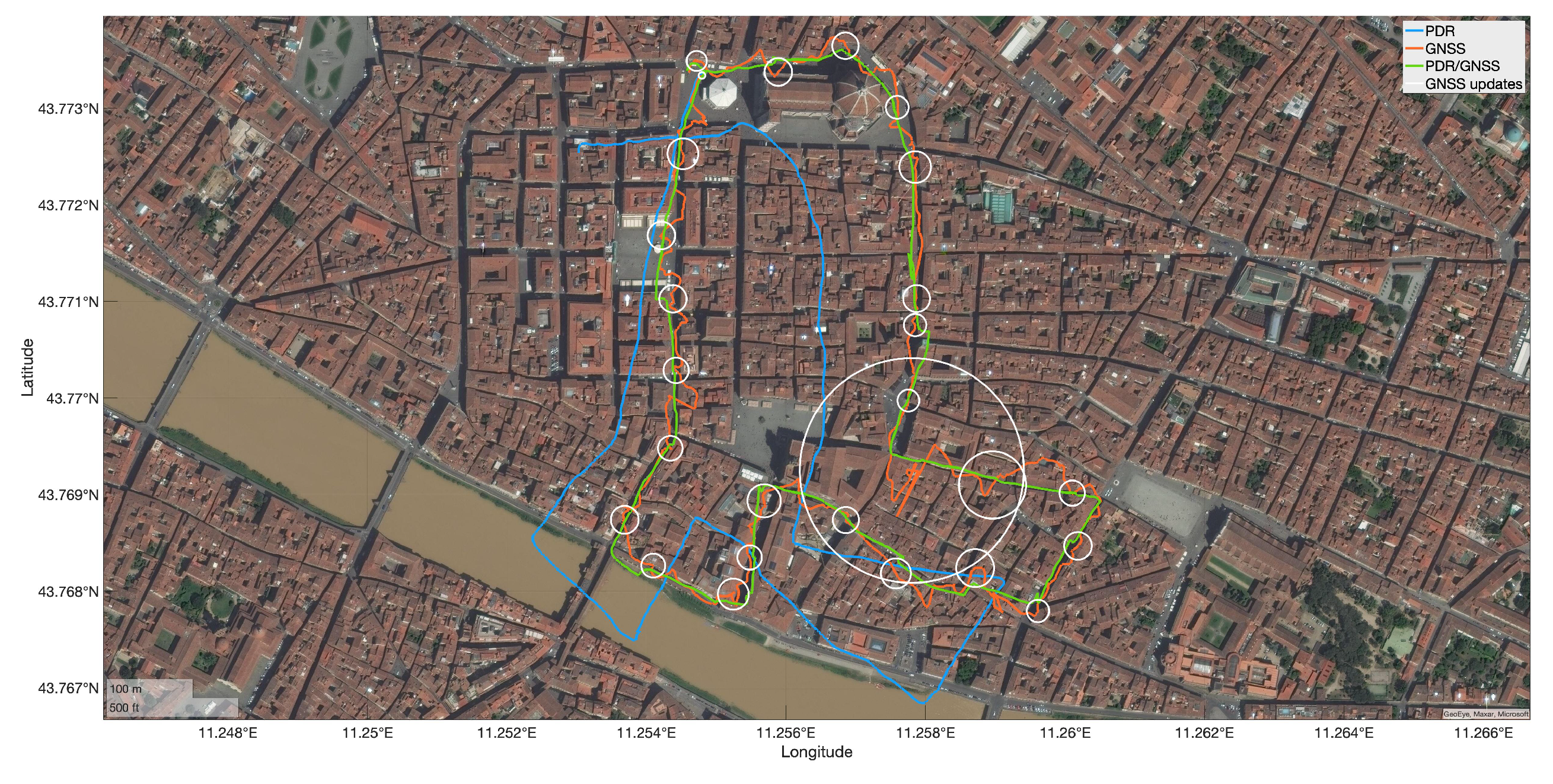
Figure 12.
Comparison between the reconstructions performed by the PDR navigation, the GNSS data and the energy saving fusion algorithm with 180 s as interval between two consecutive GNSS activations in an urban environment.
Figure 12.
Comparison between the reconstructions performed by the PDR navigation, the GNSS data and the energy saving fusion algorithm with 180 s as interval between two consecutive GNSS activations in an urban environment.

Figure 13.
Comparison between the reconstructions performed by the PDR navigation, the GNSS data and the energy saving fusion algorithm with 60 s as interval between two consecutive GNSS activations in an open space environment.
Figure 13.
Comparison between the reconstructions performed by the PDR navigation, the GNSS data and the energy saving fusion algorithm with 60 s as interval between two consecutive GNSS activations in an open space environment.


Table 1.
Technical characteristics of the smartphone used to acquire the data.
| Model | Processor | Chipset | RAM | ROM |
|---|---|---|---|---|
| Realme 5 Pro | ProKyro 360 | Snapdragon 712 | 4 GB | 128 GB |
Publisher’s Note: MDPI stays neutral with regard to jurisdictional claims in published maps and institutional affiliations. |
© 2021 by the authors. Licensee MDPI, Basel, Switzerland. This article is an open access article distributed under the terms and conditions of the Creative Commons Attribution (CC BY) license (https://creativecommons.org/licenses/by/4.0/).
Share and Cite
MDPI and ACS Style
Basso, M.; Martinelli, A.; Morosi, S.; Sera, F. A Real-Time GNSS/PDR Navigation System for Mobile Devices. Remote Sens. 2021, 13, 1567. https://0-doi-org.brum.beds.ac.uk/10.3390/rs13081567
AMA Style
Basso M, Martinelli A, Morosi S, Sera F. A Real-Time GNSS/PDR Navigation System for Mobile Devices. Remote Sensing. 2021; 13(8):1567. https://0-doi-org.brum.beds.ac.uk/10.3390/rs13081567
Chicago/Turabian StyleBasso, Michele, Alessio Martinelli, Simone Morosi, and Fabrizio Sera. 2021. "A Real-Time GNSS/PDR Navigation System for Mobile Devices" Remote Sensing 13, no. 8: 1567. https://0-doi-org.brum.beds.ac.uk/10.3390/rs13081567
Note that from the first issue of 2016, this journal uses article numbers instead of page numbers. See further details here.