
Probing the Fault Complexity of the 2017 Ms 7.0 Jiuzhaigou Earthquake Based on the InSAR Data
by
Xiongwei Tang
1,2, 
Rumeng Guo
1,2,3,*,
Jianqiao Xu
1,
Heping Sun
1,2,
Xiaodong Chen
1 and
Jiangcun Zhou
1 1
State Key Laboratory of Geodesy and Earth’s Dynamic, Innovation Academy for Precision Measurement Science and Technology, Chinese Academy of Sciences, Wuhan 430077, China
2
College of Earth and Planetary Sciences, University of Chinese Academy of Sciences, Beijing 100049, China
3
Earth System Science Programme, The Chinese University of Hong Kong, Shatin, Hong Kong, China
*
Author to whom correspondence should be addressed.
Remote Sens. 2021, 13(8), 1573; https://0-doi-org.brum.beds.ac.uk/10.3390/rs13081573
Submission received: 12 April 2021
/
Revised: 14 April 2021
/
Accepted: 15 April 2021
/
Published: 19 April 2021
Abstract
:On 8 August 2017, a surface wave magnitude (Ms) 7.0 earthquake occurred at the buried faults extending to the north of the Huya fault. Based on the coseismic deformation field obtained from interferometric synthetic aperture radar (InSAR) data and a series of finite fault model tests, we propose a brand-new two-fault model composed of a main fault and a secondary fault as the optimal model for the Jiuzhaigou earthquake, in which the secondary fault is at a wide obtuse angle to the northern end of the main fault plane. Results show that the dislocation distribution is dominated by sinistral slip, with a significant shallow slip deficit. The main fault consists of two asperities bounded by an aftershock gap, which may represent a barrier. In addition, most aftershocks are located in stress shadows and appear a complementary pattern with the coseismic high-slip regions. We propose that the aftershocks are attributable to the background tectonic stress, which may be related to the velocity-strengthening zones.
1. Introduction
On 8 August 2017, a surface wave magnitude (Ms) 7.0 earthquake occurred in Jiuzhaigou County, Aba Prefecture, Sichuan Province, China, with its epicenter at 103.82°E, 33.20°N, and a focal depth of about 20 km (Institute of Geophysics, China Earthquake Administration, CEA-IGP). As of 13 August 2017, the earthquake had caused 25 deaths and severe damage to both the Jiuzhaigou scenic area and more than 70,000 structures [1]. The Jiuzhaigou earthquake occurred near the northeastern boundary of the Bayan Har block, indicating that the Bayan Har block is still active [2]. Because the southeasterly movement of the Bayan Har block is blocked by the North China block and the South China block, there are many broom-like branches on the eastern end of the East Kunlun fault, which intersect with the Minjiang fault and the Huya fault, resulting in a complex seismic-tectonic environment in this region [3]. The NWW-trending Tazang fault, the northern segment of the NNW-trending Huya fault, and other nearby branches accommodate most of the sinistral strike-slip activity of the East Kunlun fault. The nearly NS-trending Minjiang fault and the southern segment of the Huya fault that are transverse compressional structures absorb the sinistral strike-slip motion of the remaining part of the East Kunlun fault, which causes the Minshan uplift on the eastern margin of the Tibetan Plateau [4,5].
The complicated and intense tectonic activities of these faults make the eastern margin of the Bayan Har block one of the most seismically active regions in China, with many strong earthquakes having occurred throughout its history. Examples include the 1654 Tianshui earthquake (Ms = 8), the 1879 Wudu earthquake (Ms = 7), the 1933 Diexi earthquake (Ms = 7.5), the 1976 Songpan earthquakes (Ms = 7.2, 6.7, and 7.2), the 2008 Wenchuan earthquake (Ms = 8), and the 2013 Lushan earthquake (Ms = 7) (Figure 1). The shorter duration, continuous earthquakes, and smaller strain of release compared to previous phases of earthquake clustering show that the Bayan Har block is experiencing a peak in seismic activity [4]. Therefore, further study of its seismogenic environment is urgently needed. The 2017 Jiuzhaigou earthquake provides a great opportunity to understand the tectonic loading mechanisms in this region. Different research institutions have issued a series of reports on the focal mechanisms of the Jiuzhaigou earthquake. All of them have shown that this earthquake was a sinistral strike-slip event with a high dip angle and a moment magnitude (Mw) of 6.5, but there are significant discrepancies in the fault geometry and focal depths (Table 1).
No significant coseismic surface rupture was observed for the Jiuzhaigou earthquake, making it challenging to determine the seismogenic fault [3,5]. Therefore, surface deformation as a direct response to the earthquake provides critical information for studying the seismogenic fault and rupture model. As one of the important means for obtaining surface deformation, interferometric synthetic aperture radar (InSAR) has the advantages of a wide geographical span, high precision, and high spatial resolution [7]. It is widely used to decipher earthquake cycle processes, including the interseismic locking [8], coseismic rupture [9,10], and postseismic afterslip and viscoelastic relaxation [11]. Recently, InSAR has been applied to monitor induced earthquakes, which is helpful to scientifically guide industrial production [12,13]. After the Jiuzhaigou earthquake, many studies on surface deformation and seismotectonics have been carried out using InSAR technology. Shan et al. [14] used Sentinel-1A data to acquire the coseismic surface deformation fields and inverted the rupture model. Hong et al. [15] derived the dislocation distribution from InSAR and Global Positioning System (GPS) data. Zhao et al. [16] retrieved the coseismic deformation field from Sentinel-1A InSAR data. Although a lot of research has been performed on the seismogenic fault of the Jiuzhaigou earthquake, a unified knowledge has not been achieved. From previous studies, we know that different one-fault models have a wide range of dips (50°–84°) and a small range of strikes (152°–155°) [1,5,9,14,15,16,17,18,19,20]. The two-fault models using the aftershock gap as the boundary have a small difference in fault geometry on the southern fault (strike: 145°–148°, dip: 84°–88°), but a significant difference on the northern fault (strike: 151°–171°, dip: 77°–88°) [2,21,22]. Sun et al. [10] proposed a more complex three-fault model to resolve the crustal deformation, including a fault branch forming an obtuse angle with the main subvertical fault at the northern end [23,24]. Thus, it is necessary to further discuss the seismogenic fault and rupture model of the Jiuzhaigou earthquake. Accurate coseismic slip distribution could provide a reasonable driving source for the postseismic viscoelastic relaxation analysis, Coulomb stress change assessment, and ground motion simulation. Moreover, it is of great practical significance for improving our knowledge of the background tectonics of the source region and scientifically guiding earthquake relief efforts.
In this study, four finite fault models are tested, and a brand-new two-fault model composed of a main fault and a secondary fault is finally determined as the optimal model of the 2017 Jiuzhaigou earthquake, elucidating a complex fault system. In addition, we further discuss the possible reasons for the aftershock distribution and the occurrence of the aftershock gap.
2. Data and Methods
2.1. Data
We derived the coseismic deformation field in the line-of-sight direction based on the Sentinel-1 synthetic aperture radar (SAR) images following the strategies of Ji et al. [3]. Interferometric processing was carried out using the GAMMA software. Two images, including a master image (20170730) and a slave image (20170811), from the ascending Path128 were used to obtain the interferogram based on the two-pass InSAR method [25]. The shuttle radar topography mission (SRTM) digital elevation model (DEM) with 30 m resolution was used to remove the topographic phase. In order to suppress the noise, the interferogram was multi-looked by a factor of 8 in range and 2 in azimuth and filtered twice using the weighted power spectrum algorithm with windows of 128 × 128 and then 32 × 32 pixels [26]. The minimum cost flow algorithm was used to phase unwrapping. The residual orbital phase in the interferogram was removed by a nonlinear least-squares adjustment [27]. To minimize the atmospheric signal caused by the layered atmosphere, the atmospheric delay model was established based on the existing digital elevation model and removed from the interferogram [27].
2.2. Methods
According to the Okada elastic dislocation theory [28], there is a linear relationship between the coseismic surface displacement and the fault dislocation distribution. Ideally, we would directly use the least-squares method to invert the fault dislocation distribution. However, due to practical limitations, to describe the fault more objectively, we need to discretize it into many meshes. Moreover, the distribution of the surface observation is usually heterogeneous, and the Green function matrix is often rank-deficient or ill-conditional. Generally, additional constraints are needed to ensure the stability of the inversion, and a dislocation smoothing constraint is usually used:
where , , and represent the Green function, the slip vector of each sub-fault, and the displacement vector, respectively, and is the variance between the observations and predictions. The second term is the smoothing constraint, where represents the finite difference approximation of the Laplacian operator multiplied by a weighting factor proportional to the slip amplitude, and τ is the shear stress drop that is linearly related to the slip distribution. The parameter α is the smoothing factor, which controls the trade-off between the model roughness and misfit. Generally, the “inflection point” is taken as the optimal value. We used the steepest descent method (SDM) [29,30,31,32] to estimate the slip model of the Jiuzhaigou earthquake. Compared with other inversion methods, the SDM has the advantage of providing stable inversion results with high efficiency. The Green function used for the inversion was based on the Crust1.0 layered model [33].
3. Model Tests and Results
We first constructed a one-fault model (Figure 2a) to retrieve the surface deformation. To obtain a high-resolution finite fault slip model, we divided the entire fault into 247 rectangular sub-faults with a grid of . As shown in Figure S1, we choose an optimal smoothing factor of 0.1 based on the trade-off curve. The optimal strike and dip are 154° and 51°, respectively, which is similar to the results of Shan et al. [14] (strike = 153°, dip = 50°). The one-fault model reproduces most of the observations, but it cannot decipher the surface deformation on the southeastern end of the fault satisfactorily (Table 2, Figure 3c). The slip distribution is mainly dominated by sinistral strike slips, with some thrust components on the southern segment and small normal components on the northern segment (Figure 4a). Unfortunately, this model has a significant shallow slip on the southern end of the fault, which is not consistent with the fact that there was no surface rupture.
In addition, given that the depth of the aftershocks is different in the north and the south and that there is a seismic gap [6], we also constructed a two-fault model similar to the previous studies (Figure 2b, [2,3,19,21,22,34]). The trade-off curve is shown in Figure S2a, and we set the smoothing factor as 0.15. Results demonstrate that the optimal model is composed of a northern fault (strike = 154°, dip = 66°) and a southern fault (strike = 147°, dip = 74°) (Figure S2). Our preferred strikes are similar to the model of Zheng et al. [2], and the optimal dip in the north is slightly smaller than that in the south [3,6,21,34]. Figure 3f shows that the two-fault model further improves the fit of the data (Table 2). It has a similar slip pattern to the results of joint inversion by Zheng et al. [2], whose average slip on the northern fault is larger than that on the southern fault, with a peak slip of around 0.9 m. The differences are that our results have a partial normal slip component on the northern fault, a smaller slip on the aftershock gap, and no significant slip near the surface (Figure 4b). This is consistent with the fact that the Jiuzhaigou earthquake did not result in surface rupture.
Based on the coseismic deformation field and the aftershock distribution, Sun et al. [10] proposed a fault branch at the northern end of the main fault plane at an obtuse angle. The geological survey also illustrates that there is indeed a secondary fault in this area [35]. Therefore, we introduced a similar secondary fault to construct a three-fault model (Figure 2c). During the inversion, we applied the same smoothing factor as the two-fault model. The optimal three-fault model is composed of a northern fault (strike = 156°, dip = 77°), a southern fault (strike = 145°, dip = 82°), and a secondary fault (strike = 204°, dip = 80°) (Figure S3), improving the data fit in the southwestern region compared to the two-fault model (Table 2, Figure 3h). Figure 4c shows the slip distribution, whose high-slip zone is located at a depth of 2–10 km on the main fault, with a peak slip of 1.30 m. The slip of the northern fault is composed of sinistral strike-slip and normal motion, while the southern fault is almost exclusively composed of sinistral strike-slip motion. We conclude that the average slip of the northern fault is larger than that of the southern fault, and that the secondary fault extends to the northeast of the main fault, which is consistent with the large number of aftershocks that occurred in this region.
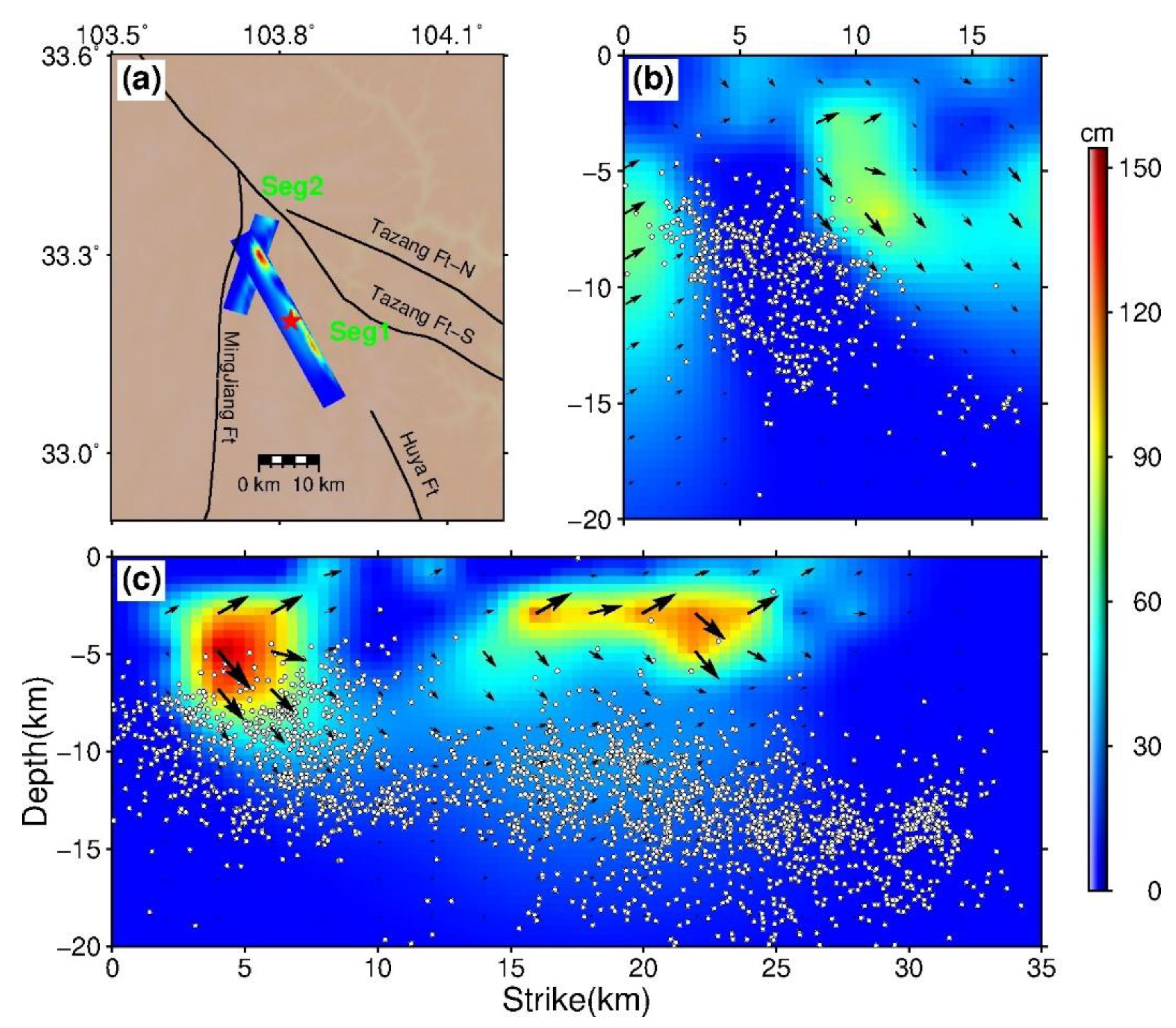
Given that the fault geometry of the southern fault is similar to that of the northern fault in the optimal three-fault model, we proposed a simpler two-fault model including a main fault and a secondary fault that is at an obtuse angle to the northern end of the main fault (Figure 2d). The trade-off curve shows that the optimal smoothing factor is consistent with the three-fault model. Figure 5 illustrates that the optimal strikes of the main fault (Seg1) and the secondary fault (Seg2) are 151° and 196°, respectively, and that their dips are both 77°. Interestingly, this brand-new two-fault model has the best fit among the four models (Table 2). The southeastern source region, which is poorly recovered by the other models, is well constrained by this model (Figure 6). Results show that the released seismic moment is around , equivalent to an Mw 6.5 event, consistent with the results of several different institutions (Table 1). Most of the coseismic slip on the main fault occurred around two shallow asperities, which are separated by a seismic gap with few aftershocks. The rupture is dominated by sinistral slip, accompanied by a small number of normal components. The high-slip regions are distributed between 2–8 km with a peak slip of 1.51 m, consistent with no surface rupture (Figure 7c). In addition, most aftershocks are concentrated under the high-slip patches and appear a complementary pattern with the coseismic slip. Interestingly, the slip on the secondary fault is also mainly concentrated in two patches, but it is separated by an aftershock swarm. They extend up to 11 km, with a peak slip of 0.85 m, coinciding with the depth of aftershocks (Figure 2d and Figure 7b). Therefore, we propose that this two-fault model is our preferred model for the Jiuzhaigou earthquake.
4. Discussion
4.1. Uncertainty Test
In order to verify the effectiveness of our preferred model, we applied the bootstrap method to estimate the uncertainty. Bootstrapping is a statistical estimation method. It randomly resamples from the original data to create multiple samples. That is, m groups of data are randomly selected from n groups of original data for inversion, and B results could be obtained by repeating the experiment B times, which allows the standard deviations to be inferred [36]. Therefore, the standard deviation obtained by the bootstrap method not only contains the influence of the original observation error, but also reflects the error caused by different data distribution. It is widely used in the estimation of model uncertainty [36,37].
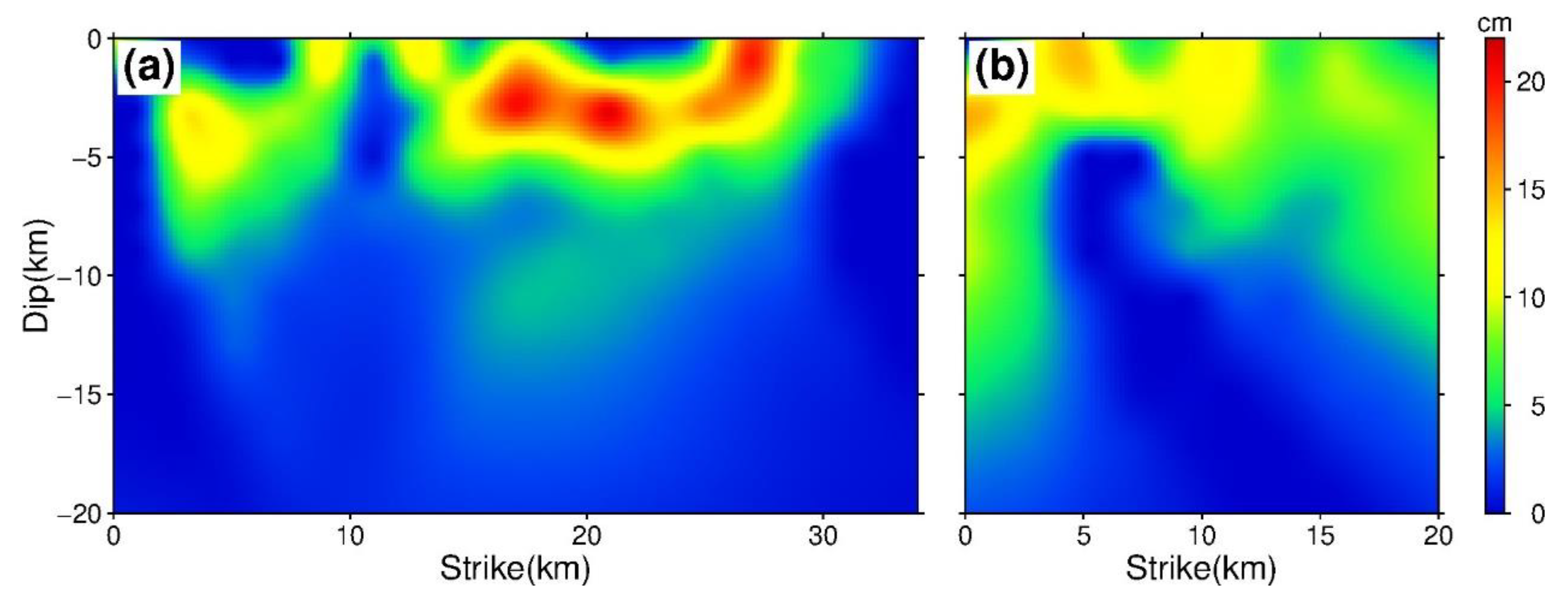
To ensure reliable results, the value of B was set to 100 [38], and corresponding resampling datasets were created in the case. These datasets were used for inversions with the same model space. Figure 8 shows the estimated uncertainties based on the bootstrap method, and the maximum standard deviation is less than 0.22 m. Although the standard deviation mainly concentrates in the southern part of the main fault, it is small relative to the peak slip of asperity. Besides, the standard deviation in the aftershock gap is very low, indicating there is indeed a slip deficit in this region. Overall, the uncertainty of our optimal two-fault model is very low, revealing the dislocation distribution is reliable and stable.
4.2. Fault Geometry and Properties
In our optimal model, the secondary fault is at a large obtuse angle to the main fault, termed backward branching. Similar phenomena were also observed in the 1992 Landers earthquake [39] and the 1999 Hector Mine earthquake [40]. The mechanism of this backward branching is the rupture stopping or slowing down on the main fault plane, which causes the rupture to jump to a nearby fault [39]. This phenomenon can also be accommodated by a significant shallow slip deficit [40]. Apparently, no significant surface rupture was observed in the Jiuzhaigou earthquake. There is a small slip zone at the south of the junction between the backward branching and the main fault, which may have been caused by a rigid block stopping or slowing down the rupture on the main fault. Moreover, the 1992 Landers earthquake and the 1999 Hector Mine earthquake both occurred within a complex fault system. The Jiuzhaigou earthquake appears to be a similar case, whose main seismogenic fault is the hidden faults with no obvious surface trace [10] or afterslip [41], indicating a young fault [10,41]. This less mature fault system is characterized by weak fault planes and more complex rupture processes.
4.3. Aftershock Distribution
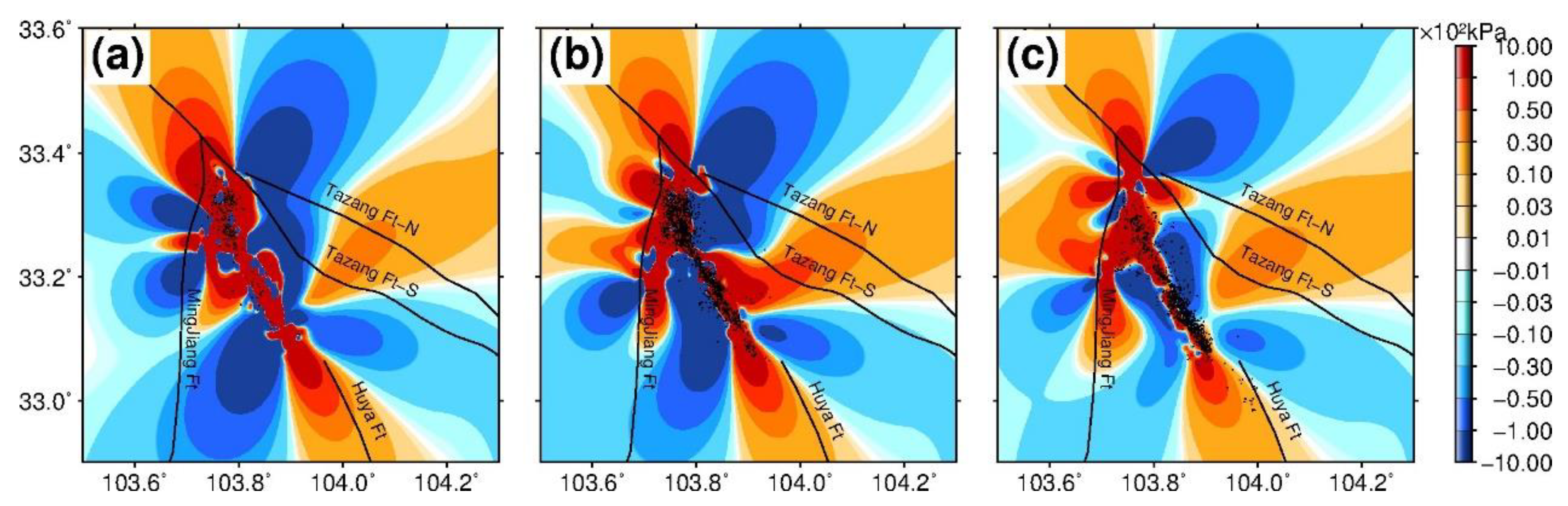
Based on the distribution of relocated aftershocks, there is an aftershock gap of around 5 km, which may be caused by one or multiple of the following three factors: (1) The coseismic slip was large and the stress release was sufficient; (2) The strikes of the faults changed at this turning point; (3) There were unbroken asperities [6]. From the InSAR surface deformation (Figure 3), we find that there are few surface deformations in the aftershock gap with the indication of no significant coseismic slip below, which is also verified by our preferred slip model. We thus rule out the first possibility. During our finite fault tests, the three-fault model suggests that the geometry parameters of the northern fault are similar to those of the southern fault, precluding the second possibility. In addition, Li et al. [41] stated that no early afterslip is observed following the Jiuzhaigou earthquake, indicating the accumulated strain is unlikely to be released by postseismic deformation in the gap. Therefore, we argue that unbroken asperities hindered the coseismic rupturing, resulting in this small seismic gap.
Figure 7 illustrates that most aftershocks occurred in the down-dip regions of the coseismic high-slip asperities, presenting a complementary pattern. Generally, it can be interpreted as (1) direct triggering from coseismic stress change [42], or (2) aftershocks that are driven by afterslip in the velocity-strengthening zone [30,43]. Therefore, we first used the numerical code PSGRN/PSCMP [44] following the strategies of Guo et al. [45] to estimate the static Coulomb stress changes caused by the coseismic slip. Since the Jiuzhaigou earthquake is a strike-slip event, we set the effective friction coefficient to 0.4 [24,45,46,47]. We used the optimal slip model as the driving source. The receiver fault was set to our preferred fault model. Results show that most aftershocks occurred in the Coulomb stress shadows (Figure S4). Therefore, we propose that the aftershock distribution may be related to aseismic afterslip, indicating the velocity-strengthening region. Further research is needed here. Helmstetter and Shaw [48] suggested that the aftershocks may be related to the tectonic stress on the fault, which could explain the inconsistency between the mechanisms of the aftershocks and that of the mainshock. Therefore, we calculated the static Coulomb stress changes on the optimally oriented failure planes for the 2017 Jiuzhaigou earthquake under the tectonic background stress field. In this study, we set the maximum principal stress, middle principal stress, and minimum principal stress to −104 kPa, −103 kPa, and 0 kPa, respectively, based on previous studies [23,24]. Although the tectonic stresses may have large uncertainties, it does not prevent us from analyzing them rationally. Figure 9 reveals the static Coulomb stress changes at different depths and the distribution of the aftershocks within 5 km, from which we find that most of the aftershocks occurred in the region where the Coulomb stress increased. Therefore, the aftershocks of the Jiuzhaigou earthquake may have been controlled by the background tectonic stress field.
5. Conclusions
In this study, we tested four different finite fault models based on the InSAR data, and determined that the seismogenic fault of the 2017 Mw 6.5 Jiuzhaigou earthquake was a brand-new two-fault model. The high-slip regions in the main fault are distributed between 2–8 km, with a peak slip of 1.51 m. There are two asperities that are perfectly demarcated by the aftershock gap, which may indicate a barrier. The secondary fault is at a large obtuse angle to the main fault, whose slip extends to 11 km, with a peak slip at 0.85 m. The main fault of the Jiuzhaigou earthquake is the NW-trending hidden fault of the Huya fault, which is one of the branches of the East Kunlun fault. There were a few aftershocks at both ends of the main fault where the Coulomb stress increased, which deserve our particular attention.
Supplementary Materials
The following are available online at https://0-www-mdpi-com.brum.beds.ac.uk/article/10.3390/rs13081573/s1, Figure S1—Search results of the one-fault model; Figure S2—Search results of the two-fault model; Figure S3—Search results of the three-fault model; Figure S4—Static Coulomb stress changes caused by the Jiuzhaigou earthquake at different depths and the distribution of the aftershocks within 5 km.
Author Contributions
Conceptualization, R.G. and X.T.; methodology, J.X.; software, R.G.; validation, J.X., R.G., H.S., X.C. and J.Z.; formal analysis, R.G.; writing—original draft preparation, X.T.; writing—review and editing, X.T., J.X., R.G., H.S., X.C. and J.Z.; visualization, X.T. and R.G.; supervision, J.X., H.S., X.C. and J.Z.; project administration, X.C. and J.Z.; funding acquisition, J.X., H.S., X.C. and J.Z. All authors have read and agreed to the published version of the manuscript.
Funding
This research was funded by the B-type Strategic Priority Program of the Chinese Academy of Sciences, grant number XDB41000000, and the National Natural Science Foundation of China, grant numbers 41974023, 41874094, 41674083, 41874026.
Institutional Review Board Statement
Not applicable.
Informed Consent Statement
Not applicable.
Data Availability Statement
Not applicable.
Acknowledgments
We thank the National Earth System Science Data Center, National Science & Technology Infrastructure of China (http://www.geodata.cn, accessed on 14 April 2021) for the data provided. We are grateful to Lingyun Ji of the Second Monitoring Center, China Earthquake Administration for providing the InSAR data. We used the Generic Mapping Tools (GMT) open-source collection of computer software tools to create the figures, which is developed and maintained by Paul Wessel and Walter H. F. Smith.
Conflicts of Interest
The authors declare no conflict of interest.
References
- Li, Q.; Tan, K.; Wang, D.Z.; Zhao, B.; Zhang, R.; Li, Y.; Qi, Y.J. Joint inversion of GNSS and teleseismic data for the rupture process of the 2017 Mw6.5 Jiuzhaigou, China, earthquake. J. Seism. 2018, 22, 805–814. [Google Scholar] [CrossRef]
- Zheng, A.; Yu, X.; Xu, W.; Chen, X.; Zhang, W. A hybrid source mechanism of the 2017 Mw 6.5 Jiuzhaigou earthquake revealed by the joint inversion of strong-motion, teleseismic and InSAR data. Tectonophysics 2020, 789, 228538. [Google Scholar] [CrossRef]
- Ji, L.; Liu, C.; Xu, J.; Liu, L.; Long, F.; Zhang, Z. InSAR observation and inversion of the seismogenic fault for the 2017 Jiuzhaigou MS7.0 earthquake in China. Chin. J. Geophys. 2017, 60, 4069–4082. [Google Scholar]
- Deng, Q.; Cheng, S.; Ma, J.; Du, P. Seismic activities and earthquake potential in the Tibetan Plateau. Chin. J. Geophys. 2014, 57, 2025–2042. [Google Scholar]
- Xu, X.; Chen, G.; Wang, Q.; Chen, L.; Ren, Z.; Xu, C.; Wei, Z.; Lu, R.; Tan, X.; Dong, S.; et al. Discussion on seismogenic structure of Jiuzhaigou earthquake and its implication for current strain state in the southeastern Qinghai-Tibet Plateau. Chin. J. Geophys. 2017, 60, 4018–4026. [Google Scholar]
- Fang, L.; Wu, J.; Su, J.; Wang, M.; Jiang, C.; Fan, L.; Wang, W.; Wang, C.; Tan, X. Relocation of mainshock and aftershock sequence of the Ms7.0 Sichuan Jiuzhaigou earthquake. Chin. Sci. Bull. 2018, 63, 649–662. [Google Scholar] [CrossRef] [Green Version]
- Zebker, H.A.; Rosen, P.A.; Goldstein, R.M.; Gabriel, A.; Werner, C.L. On the derivation of coseismic displacement fields using differential radar interferometry: The Landers earthquake. J. Geophys. Res. Space Phys. 1994, 99, 19617–19634. [Google Scholar] [CrossRef]
- Hussain, E.; Wright, T.J.; Walters, R.J.; Bekaert, D.P.S.; Lloyd, R.; Hooper, A. Constant strain accumulation rate between major earthquakes on the North Anatolian Fault. Nat. Commun. 2018, 9, 1–9. [Google Scholar] [CrossRef]
- Nie, Z.; Wang, D.-J.; Jia, Z.; Yu, P.; Li, L. Fault model of the 2017 Jiuzhaigou Mw 6.5 earthquake estimated from coseismic deformation observed using Global Positioning System and Interferometric Synthetic Aperture Radar data. Earthplanets Space 2018, 70, 55. [Google Scholar] [CrossRef] [Green Version]
- Sun, J.; Yue, H.; Shen, Z.; Fang, L.; Zhan, Y.; Sun, X. The 2017 Jiuzhaigou Earthquake: A Complicated Event Occurred in a Young Fault System. Geophys. Res. Lett. 2018, 45, 2230–2240. [Google Scholar] [CrossRef]
- Zhao, D.; Qu, C.; Bürgmann, R.; Gong, W.; Shan, X. Relaxation of Tibetan Lower Crust and Afterslip Driven by the 2001 Mw7.8 Kokoxili, China, Earthquake Constrained by a Decade of Geodetic Measurements. J. Geophys. Res. Solid Earth 2021, 126. [Google Scholar] [CrossRef]
- Malinowska, A.A.; Witkowski, W.T.; Guzy, A.; Hejmanowski, R. Mapping ground movements caused by mining-induced earthquakes applying satellite radar interferometry. Eng. Geol. 2018, 246, 402–411. [Google Scholar] [CrossRef]
- Sopata, P.; Stoch, T.; Wójcik, A.; Mrocheń, D. Land Surface Subsidence Due to Mining-Induced Tremors in the Upper Silesian Coal Basin (Poland)—Case Study. Remote Sens. 2020, 12, 3923. [Google Scholar] [CrossRef]
- Shan, X.; Qu, C.; Gong, W.; Zhao, D.; Zhang, G. Coseismic deformation field of the Jiuzhaigou MS7.0 earthquake from Sentinel-1A InSAR data and fault slip inversion. Chin. J. Geophys. 2017, 60, 4527–4536. [Google Scholar]
- Hong, S.; Zhou, X.; Zhang, K.; Meng, G.; Dong, Y.; Su, X.; Zhang, L.; Li, S.; Ding, K. Source Model and Stress Disturbance of the 2017 Jiuzhaigou Mw 6.5 Earthquake Constrained by InSAR and GPS Measurements. Remote Sens. 2018, 10, 1400. [Google Scholar] [CrossRef] [Green Version]
- Zhao, D.; Qu, C.; Shan, X.; Gong, W.; Zhang, Y.; Zhang, G. InSAR and GPS derived coseismic deformation and fault model of the 2017 Ms7.0 Jiuzhaigou earthquake in the Northeast Bayanhar block. Tectonophyicsics 2018, 726, 86–99. [Google Scholar] [CrossRef]
- Chen, W.; Qiao, X.J.; Liu, G.; Xiong, W.; Jia, Z.G.; Li, Y.; Wang, Y.B.; You, Z.L.; Long, F. Study on the coseismic slip model and Coulomb stress of the 2017 Jiuzhaigou MS7.0 earthquake constrained by GNSS and InSAR measurements. Chin. J. Geophys. 2018, 61, 2122–2132. [Google Scholar]
- Shen, W.; Li, Y.S.; Jiao, Q.; Xie, Q.; Zhang, J. Joint inversion of strong motion and InSAR/GPS data for fault slip distribution of the Jiuzhaigou 7.0 earthquake and its application in seismology. Chin. J. Geophys. 2019, 61, 115–129. [Google Scholar]
- Xie, Z.; Zheng, Y.; Yao, H.; Fang, L.; Liu, C.; Wang, M.; Shan, B.; Zhang, H.; Ren, J.; Ji, L.; et al. Preliminary analysis on the source properties and seismogenic structure of the 2017 Ms7.0 Jiuzhaigou earthquake. Sci. China Earth Sci. 2018, 61, 339–352. [Google Scholar] [CrossRef]
- Gui-Xi, Y.; Feng, L.; Ming-Jian, L.; Hui-Ping, Z.; Min, Z.; You-Qing, Y.; Zhi-Wei, Z.; Yu-Ping, Q.; Si-Wei, W.; Yue, G.; et al. Focal mechanism solutions and seismogenic structure of the 8 August 2017 M7.0 Jiuzhaigou earthquake and its aftershocks, northern Sichuan. Chin. J. Geophys. 2017, 60, 4083–4097. [Google Scholar]
- Hu, X.; Sheng, S.; Wang, Y.; Liang, S. Fault Plane Parameters of 2017 Jiuzhaigou Ms7. 0 Earthquake Determined by Aftershock Distribution. J. Seismol. Res. 2019, 42, 366–371. [Google Scholar]
- Liu, G.; Xiong, W.; Wang, Q.; Qiao, X.; Ding, K.; Li, X.; Yang, S. Source Characteristics of the 2017 Ms 7.0 Jiuzhaigou, China, Earthquake and Implications for Recent Seismicity in Eastern Tibet. J. Geophys. Res. Solid Earth 2019, 124, 4895–4915. [Google Scholar] [CrossRef]
- Toda, S.; Stein, R.S.; Richards-Dinger, K.; Bozkurt, S.B. Forecasting the evolution of seismicity in southern California: Animations built on earthquake stress transfer. J. Geophys. Res. Space Phys. 2005, 110, 1–17. [Google Scholar] [CrossRef]
- Wang, J.; Xu, C. Coseismic Coulomb stress changes associated with the 2017 MW6.5 Jiuzhaigou earthquake (China) and its impacts on surrounding major faults. Chin. J. Geophys. 2017, 60, 4398–4420. [Google Scholar]
- Massonnet, D.; Feigl, K.L. Radar interferometry and its application to changes in the Earth’s surface. Rev. Geophys. 1998, 4, 441–500. [Google Scholar] [CrossRef] [Green Version]
- Goldstein, R.M.; Werner, C.L. Radar interferogram filtering for geophysical applications. Geophys. Res. Lett. 1998, 25, 4035–4038. [Google Scholar] [CrossRef] [Green Version]
- Rosen, P.A.; Hensley, S.; Zebker, H.A.; Webb, F.H.; Fielding, E.J. Surface deformation and coherence measurements of Kilauea Volcano, Hawaii, from SIR-C radar interferometry. J. Geophys. Res. Space Phys. 1996, 101, 23109–23125. [Google Scholar] [CrossRef]
- Okada, Y. Surface deformation due to shear and tensile faults in a half-space. B Seismol. Soc. Am. 1985, 75, 1135–1154. [Google Scholar]
- Guo, R.; Zheng, Y.; Diao, F.; Xu, J. Rupture model of the 2013 M W 6.6 Lushan (China) earthquake constrained by a new GPS data set and its effects on potential seismic hazard. Earthq. Sci. 2018, 31, 117–125. [Google Scholar]
- Guo, R.; Zheng, Y.; Xu, J.; Jiang, Z. Seismic and Aseismic Fault Slip Associated with the 2017 M w 8.2 Chiapas, Mexico, Earthquake Sequence. Seismol. Res. Lett. 2019, 90, 1111–1120. [Google Scholar] [CrossRef]
- Wang, R.; Diao, F.; Hoechner, A. SDM—A geodetic inversion code incorporating with layered crust structure and curved fault geometry. In Proceedings of the EGU General Assembly 2013, Vienna, Austria, 7–12 April 2013. [Google Scholar]
- Wang, R.; Martín, F.L.; Roth, F. Computation of deformation induced by earthquakes in a multi-layered elastic crust—FORTRAN programs EDGRN/EDCMP. Comput. Geosci. UK 2003, 29, 195–207. [Google Scholar] [CrossRef]
- Laske, G.; Masters, G.; Ma, Z.; Pasyanos, M.E. CRUST1.0: An updated global model of Earth’s crust. In Proceedings of the EGU General Assembly 2012, Vienna, Austria, 22–27 April 2012. [Google Scholar]
- Wang, Y.; Zhao, T.; Li, C.X.; Liu, C. Relocations and focal mechanism solutions of the 2017 Jiuzhaigou, Sichuan MS 7.0 earthquake sequence. Process Geophys. 2019, 34, 469–478. [Google Scholar]
- Yi, S.-J.; Wu, C.-H.; Li, Y.-S.; Huang, C. Source tectonic dynamics features of Jiuzhaigou Ms 7.0 earthquake in Sichuan Province, China. J. Mt. Sci. 2018, 15, 2266–2275. [Google Scholar] [CrossRef]
- Schnaidt, S.; Heinson, G. Bootstrap resampling as a tool for uncertainty analysis in 2-D magnetotelluric inversion modelling. Geophys. J. Int. 2015, 203, 92–106. [Google Scholar] [CrossRef] [Green Version]
- McLaughlin, K.L. Maximum-likelihood event magnitude estimation with bootstrapping for uncertainty estimation. B Seismol. Soc. Am. 1988, 78, 855–862. [Google Scholar]
- Efron, B.; Tibshirani, R. Bootstrap Methods for Standard Errors, Confidence Intervals, and Other Measures of Statistical Accuracy. Stat. Sci. 1986, 1, 54–75. [Google Scholar] [CrossRef]
- Fliss, S.; Bhat, H.S.; Dmowska, R.; Rice, J.R. Fault branching and rupture directivity. J. Geophys. Res. Space Phys. 2005, 110, 110. [Google Scholar] [CrossRef] [Green Version]
- Oglesby, D.D.; Day, S.M.; Li, Y.; Vidale, J.E. The 1999 Hector Mine Earthquake: The Dynamics of a Branched Fault System. B. Seismol. Soc. Am. 2003, 93, 2459–2476. [Google Scholar] [CrossRef]
- Li, Y.; Bürgmann, R.; Zhao, B. Evidence of Fault Immaturity from Shallow Slip Deficit and Lack of Postseismic Deformation of the 2017 Mw 6.5 Jiuzhaigou Earthquake. Bull. Seism. Soc. Am. 2020, 110, 154–165. [Google Scholar] [CrossRef]
- Stein, R.S.; King, G.C.P.; Lin, J. Stress Triggering of the 1994 M = 6.7 Northridge, California, Earthquake by Its Predecessors. Science 1994, 265, 1432–1435. [Google Scholar] [CrossRef]
- Guo, R.; Zheng, Y.; An, C.; Xu, J.; Jiang, Z.; Zhang, L.; Riaz, M.S.; Xie, J.; Dai, K.; Wen, Y. The 2018 Mw 7.9 Offshore Kodiak, Alaska, Earthquake: An Unusual Outer Rise Strike-Slip Earthquake. J. Geophys. Res. Solid Earth 2020, 125, e2019JB019267. [Google Scholar]
- Wang, R.; Lorenzo-Martín, F.; Roth, F. PSGRN/PSCMP—a new code for calculating co- and post-seismic deformation, geoid and gravity changes based on the viscoelastic-gravitational dislocation theory. Comput. Geosci. 2006, 32, 527–541. [Google Scholar] [CrossRef] [Green Version]
- Guo, R.; Zheng, Y.; Xu, J. Stress modulation of the seismic gap between the 2008 M s 8.0 Wenchuan earthquake and the 2013 M s 7.0 Lushan earthquake and implications for seismic hazard. Geophys. J. Int. 2020, 221, 2113–2125. [Google Scholar] [CrossRef]
- Lin, X.; Chu, R.; Zeng, X. Rupture processes and Coulomb stress changes of the 2017 Mw 6.5 Jiuzhaigou and 2013 Mw 6.6 Lushan earthquakes. Earthplanets Space 2019, 71, 1–15. [Google Scholar] [CrossRef]
- Shan, B.; Zheng, Y.; Liu, C.; Xie, Z.; Kong, J. Coseismic Coulomb failure stress changes caused by the 2017 M7.0 Jiuzhaigou earthquake, and its relationship with the 2008 Wenchuan earthquake. Sci. China Earth Sci. 2017, 60, 2181–2189. [Google Scholar] [CrossRef]
- Helmstetter, A.; Shaw, B.E. Relation between stress heterogeneity and aftershock rate in the rate-and-state model. J. Geophys. Res. Space Phys. 2006, 111. [Google Scholar] [CrossRef]
Figure 1.
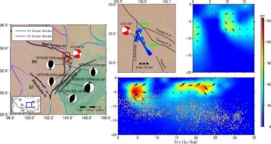
Tectonic setting and seismicity around the 2017 Jiuzhaigou earthquake. (a) Tectonic setting of the eastern margin of the Tibetan Plateau. The solid blue and purple lines indicate the primary and secondary block boundaries, respectively. The color-coded circles represent historical earthquakes () from the Data Sharing Infrastructure of National Earthquake Data Center (NEDC) (http://data.earthquake.cn, accessed on 14 April 2021). The black beach balls show the focal mechanisms of the historical earthquakes () in this region from the Global Centroid Moment Tensor, Harvard University Global Moment Tensor Solution (GCMT). The red beach ball represents the focal mechanism of the Jiuzhaigou earthquake from the Institute of Geophysics, China Earthquake Administration (CEA-IGP) (http://www.cea-igp.ac.cn/en/, accessed on 14 April 2021). The inset shows the large-scale tectonic environment. The red rectangle is the region shown in (b). Note: QT—Qiangtang block; BH—Bayan Har block; QL—Qilian block; SC—South China; NC—North China; TB—Tibet; TR—Tarim Basin. (b) Fault geometry and aftershocks of the Jiuzhaigou earthquake. The blue dots are the relocated aftershocks within a month from Fang et al. [6], and the red rectangle is the projection of our optimal fault model on the surface. The gray, black, red, and purple beach balls show the focal mechanisms determined by the GCMT, United States Geological Survey (USGS) (https://www.usgs.gov/, accessed on 14 April 2021), CEA-IGP, and Institute of Earthquake Forecasting, China Earthquake Administration (CEA-IEF) (http://www.ief.ac.cn/, accessed on 14 April 2021), respectively.
Figure 1.
Tectonic setting and seismicity around the 2017 Jiuzhaigou earthquake. (a) Tectonic setting of the eastern margin of the Tibetan Plateau. The solid blue and purple lines indicate the primary and secondary block boundaries, respectively. The color-coded circles represent historical earthquakes () from the Data Sharing Infrastructure of National Earthquake Data Center (NEDC) (http://data.earthquake.cn, accessed on 14 April 2021). The black beach balls show the focal mechanisms of the historical earthquakes () in this region from the Global Centroid Moment Tensor, Harvard University Global Moment Tensor Solution (GCMT). The red beach ball represents the focal mechanism of the Jiuzhaigou earthquake from the Institute of Geophysics, China Earthquake Administration (CEA-IGP) (http://www.cea-igp.ac.cn/en/, accessed on 14 April 2021). The inset shows the large-scale tectonic environment. The red rectangle is the region shown in (b). Note: QT—Qiangtang block; BH—Bayan Har block; QL—Qilian block; SC—South China; NC—North China; TB—Tibet; TR—Tarim Basin. (b) Fault geometry and aftershocks of the Jiuzhaigou earthquake. The blue dots are the relocated aftershocks within a month from Fang et al. [6], and the red rectangle is the projection of our optimal fault model on the surface. The gray, black, red, and purple beach balls show the focal mechanisms determined by the GCMT, United States Geological Survey (USGS) (https://www.usgs.gov/, accessed on 14 April 2021), CEA-IGP, and Institute of Earthquake Forecasting, China Earthquake Administration (CEA-IEF) (http://www.ief.ac.cn/, accessed on 14 April 2021), respectively.

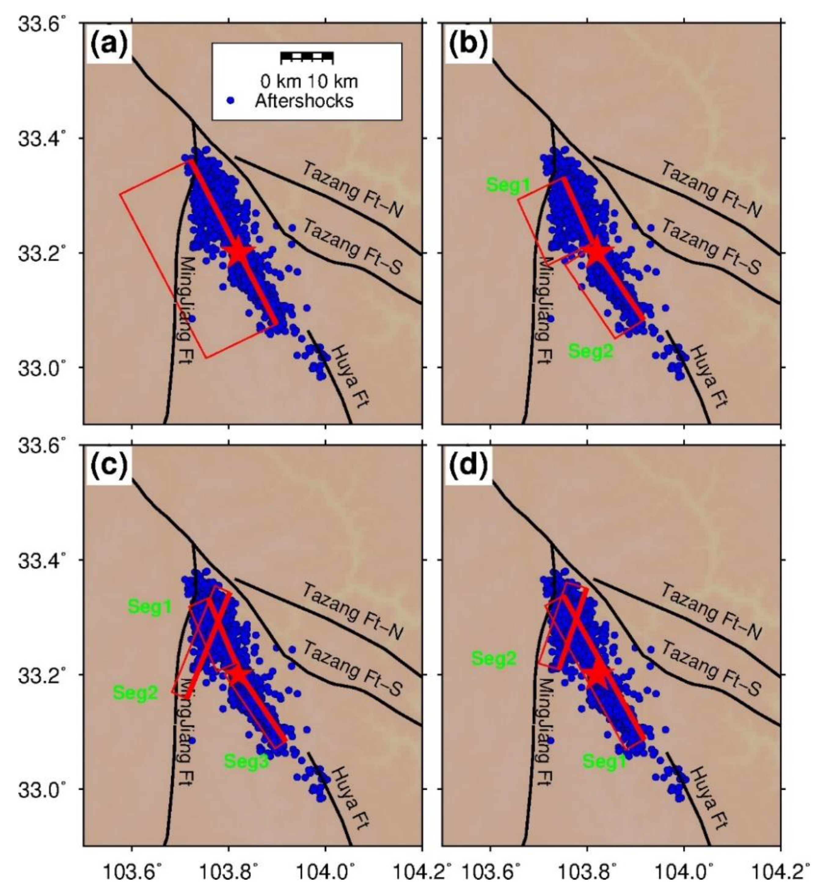
Figure 2.
Projections of the four finite fault models on the surface, including the (a) one-fault model, (b) two-fault model (a northern fault and a southern fault), (c) three-fault model, and (d) brand-new two-fault model (a main fault and a secondary fault). Other symbols are the same as Figure 1b.

Figure 3.
Comparison between interferometric synthetic aperture radar (InSAR) observations and predictions from the three test models. (a,d,g) Coseismic line-of-sight (LOS) deformation. Simulated LOS deformation from the (b) one-fault model, (e) two-fault model, and (h) three-fault model. (c,f,i) Residuals. Red star represents the epicenter of the 2017 Jiuzhaigou earthquake from the CEA-IGP.

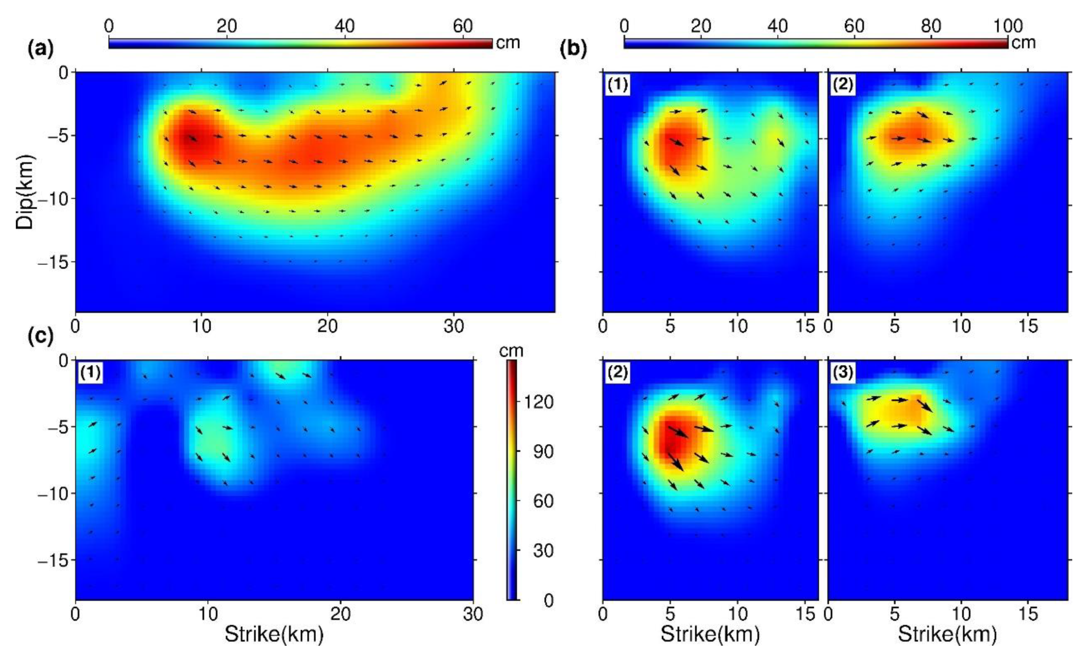
Figure 4.
Slip distribution with arrows delineating the average rake of each sub-fault for the three test models, whose magnitude is color-coded. (a) Slip distribution for the optimal one-fault model. (b) Slip distribution for the optimal two-fault model, including the (1) northern fault and (2) southern fault. (c) Slip distribution for the optimal three-fault model, including the (1) secondary fault, (2) northern fault, and (3) southern fault.

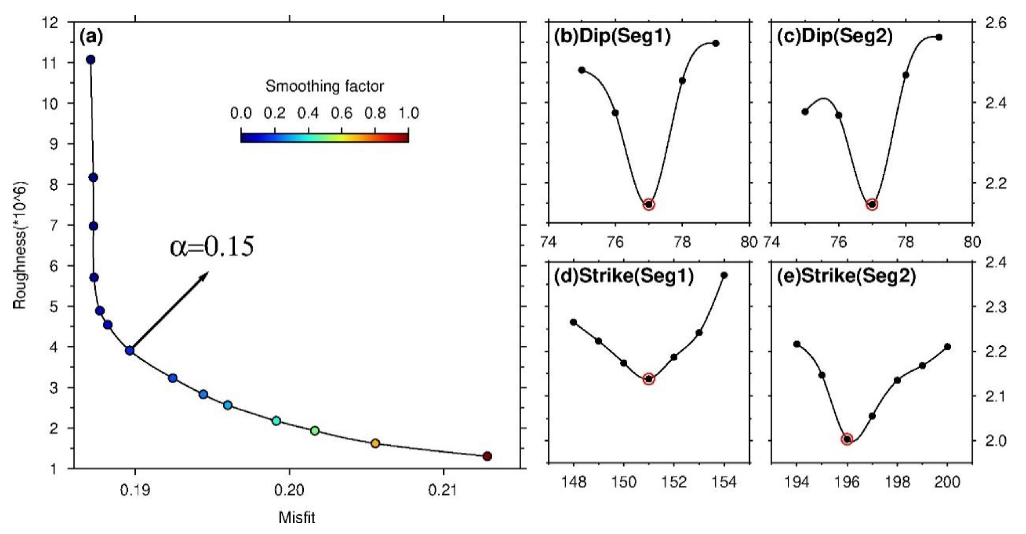
Figure 5.
Search results of our preferred model. (a) Trade-off curve between the model roughness and misfit. Dips of the (b) main fault (Seg1) and (c) secondary fault (Seg2). Strikes of the (d) main fault (Seg1) and (e) secondary fault (Seg2).
Figure 5.
Search results of our preferred model. (a) Trade-off curve between the model roughness and misfit. Dips of the (b) main fault (Seg1) and (c) secondary fault (Seg2). Strikes of the (d) main fault (Seg1) and (e) secondary fault (Seg2).

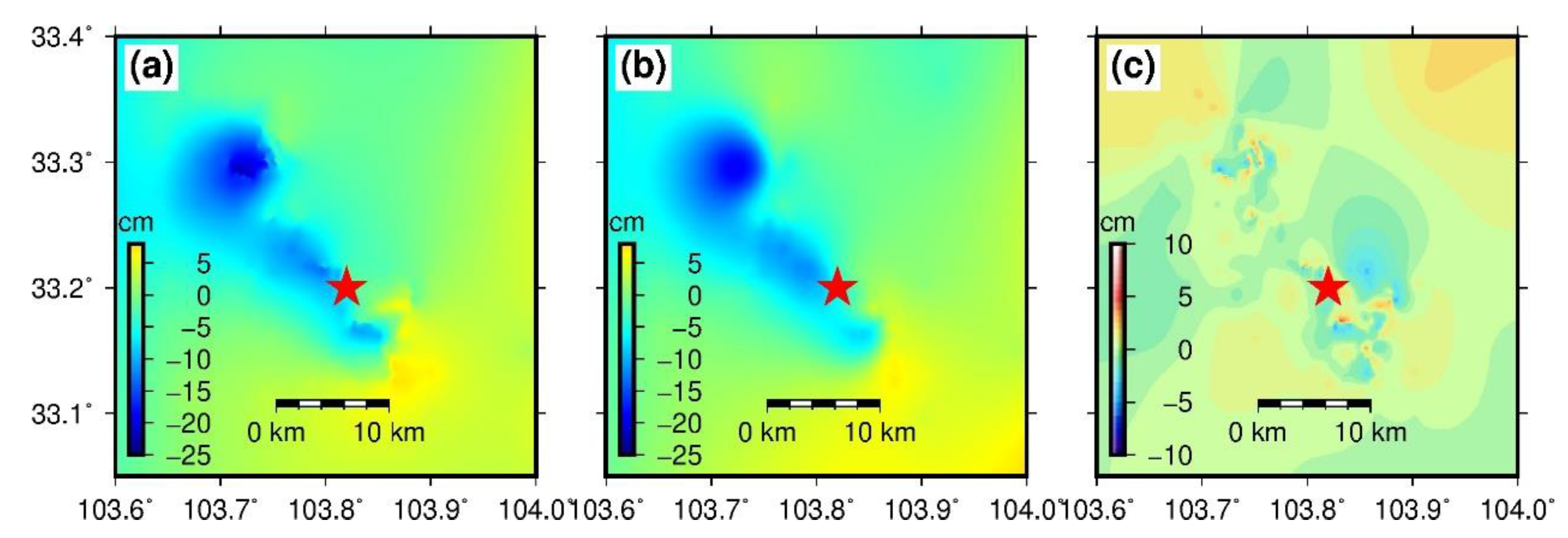
Figure 6.
Comparison between InSAR observations and predictions from our preferred model. (a) Coseismic LOS deformation. (b) Simulated LOS deformation. (c) Residuals. Other symbols are the same as Figure 3.
Figure 6.
Comparison between InSAR observations and predictions from our preferred model. (a) Coseismic LOS deformation. (b) Simulated LOS deformation. (c) Residuals. Other symbols are the same as Figure 3.

Figure 7.
Slip distribution for our preferred model. (a) Projection of the slip model on the surface. Slip distribution of the (b) secondary fault, and (c) main fault. The white dots represent the relocated aftershocks. The slip distribution with arrows delineating the average rake of each sub-fault is color-coded. Other symbols are the same as Figure 1b.

Figure 8.
The standard deviations of the (a) main fault, and (b) secondary fault, based on the bootstrap method.
Figure 8.
The standard deviations of the (a) main fault, and (b) secondary fault, based on the bootstrap method.

Figure 9.
Static Coulomb stress changes on the 3D optimally oriented failure planes created by the Jiuzhaigou earthquake at different depths and the distribution of the aftershocks within 5 km. Coulomb stress changes at a depth of (a) 5 km, (b) 10 km, and (c) 15 km. Black dots represent the relocated aftershocks.


Table 1.
Focal mechanisms of the 2017 Jiuzhaigou earthquake determined by different institutions.
| Nodal Plane I | Nodal Plane II | Magnitude (Mw) | Depth (km) | |
|---|---|---|---|---|
| Strike, Dip, Rake | Strike, Dip, Rake | |||
| GCMT | 242°, 77°, −168° | 150°, 78°, −13° | 6.5 | 14.9 |
| USGS | 246°, 57°, −173° | 153°, 84°, −33° | 6.5 | 13.5 |
| CEA-IGP | 328°, 48°, −11° | 65°, 82°, 137° | 6.5 | 20.0 |
| CEA-IEF | 59°, 77°, 164° | 152°, 75°, 13° | 6.5 | 5.0 |
Table 2.
Parameters of finite fault models.
| Faults | Strike | Dip | Average Error (m) | Maximum Residual (m) | ||
|---|---|---|---|---|---|---|
| One-fault | Main fault | 154° | 51° | 0.0211 | −0.0900 | 6.4 |
| Two-fault | Northern fault | 154° | 66° | 0.0203 | −0.0684 | 6.4 |
| Southern fault | 147° | 74° | ||||
| Three-fault | Northern fault | 156° | 77° | 0.0198 | −0.0602 | 6.4 |
| Southern fault | 147° | 82° | ||||
| Secondary fault | 204° | 80° | ||||
| New two-fault | Main fault | 151° | 77° | 0.0188 | −0.0487 | 6.5 |
| Secondary fault | 196° | 77° |
Publisher’s Note: MDPI stays neutral with regard to jurisdictional claims in published maps and institutional affiliations. |
© 2021 by the authors. Licensee MDPI, Basel, Switzerland. This article is an open access article distributed under the terms and conditions of the Creative Commons Attribution (CC BY) license (https://creativecommons.org/licenses/by/4.0/).
Share and Cite
MDPI and ACS Style
Tang, X.; Guo, R.; Xu, J.; Sun, H.; Chen, X.; Zhou, J. Probing the Fault Complexity of the 2017 Ms 7.0 Jiuzhaigou Earthquake Based on the InSAR Data. Remote Sens. 2021, 13, 1573. https://0-doi-org.brum.beds.ac.uk/10.3390/rs13081573
AMA Style
Tang X, Guo R, Xu J, Sun H, Chen X, Zhou J. Probing the Fault Complexity of the 2017 Ms 7.0 Jiuzhaigou Earthquake Based on the InSAR Data. Remote Sensing. 2021; 13(8):1573. https://0-doi-org.brum.beds.ac.uk/10.3390/rs13081573
Chicago/Turabian StyleTang, Xiongwei, Rumeng Guo, Jianqiao Xu, Heping Sun, Xiaodong Chen, and Jiangcun Zhou. 2021. "Probing the Fault Complexity of the 2017 Ms 7.0 Jiuzhaigou Earthquake Based on the InSAR Data" Remote Sensing 13, no. 8: 1573. https://0-doi-org.brum.beds.ac.uk/10.3390/rs13081573
Note that from the first issue of 2016, this journal uses article numbers instead of page numbers. See further details here.