
Decision-Level and Feature-Level Integration of Remote Sensing and Geospatial Big Data for Urban Land Use Mapping

 ,
,  and
and
Abstract
:1. Introduction
2. Related Work of RS and GBD Integration Used in Urban Land Use Mapping
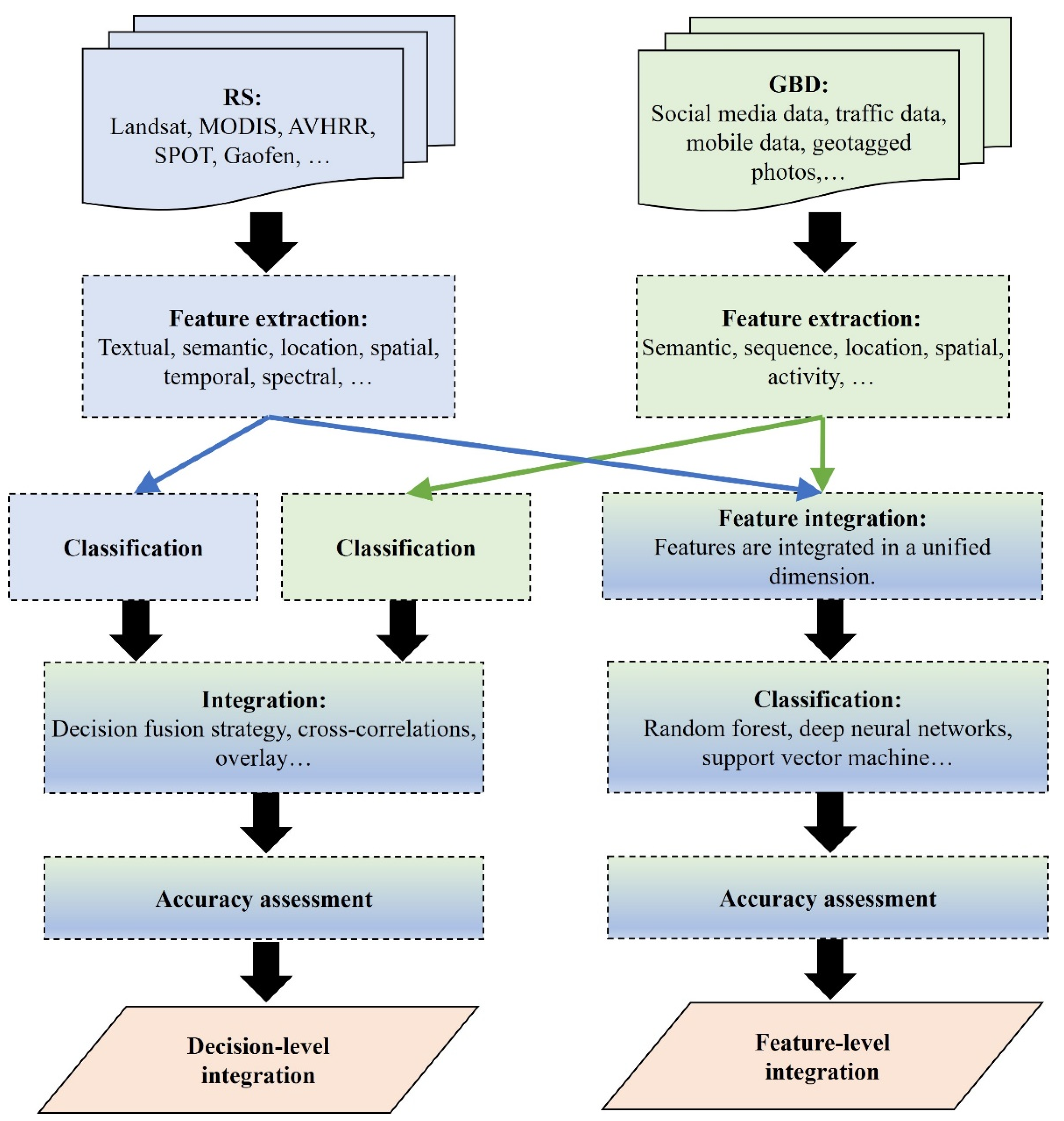
2.1. DI-Based Urban Land Use Mapping
2.2. FI-Based Urban Land Use Mapping
3. Case Study
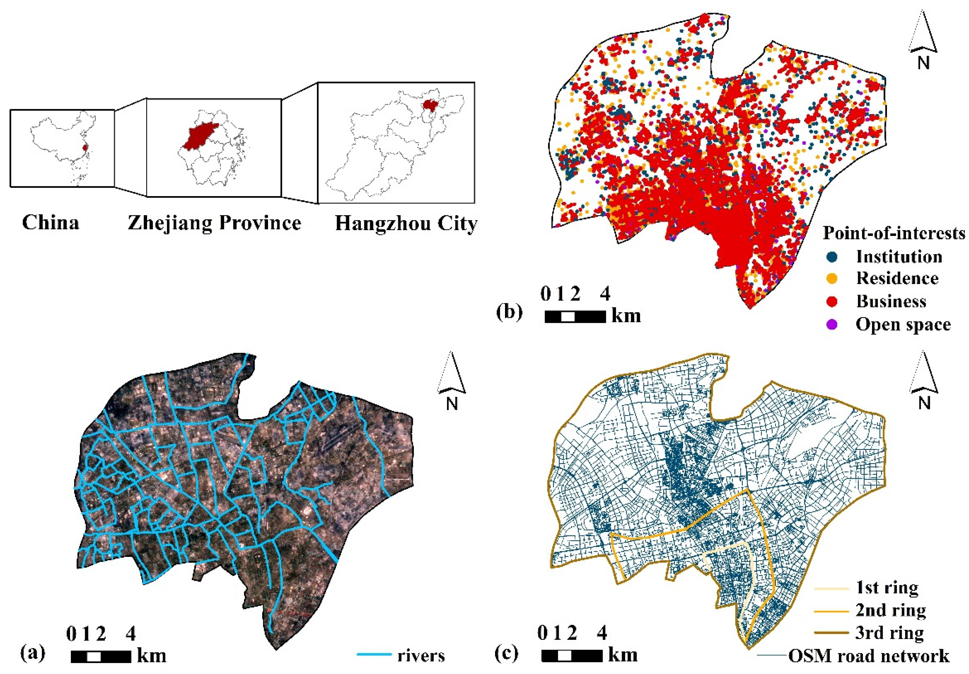
3.1. Study Site
3.2. Data Source and Preprocessing
3.3. Methods
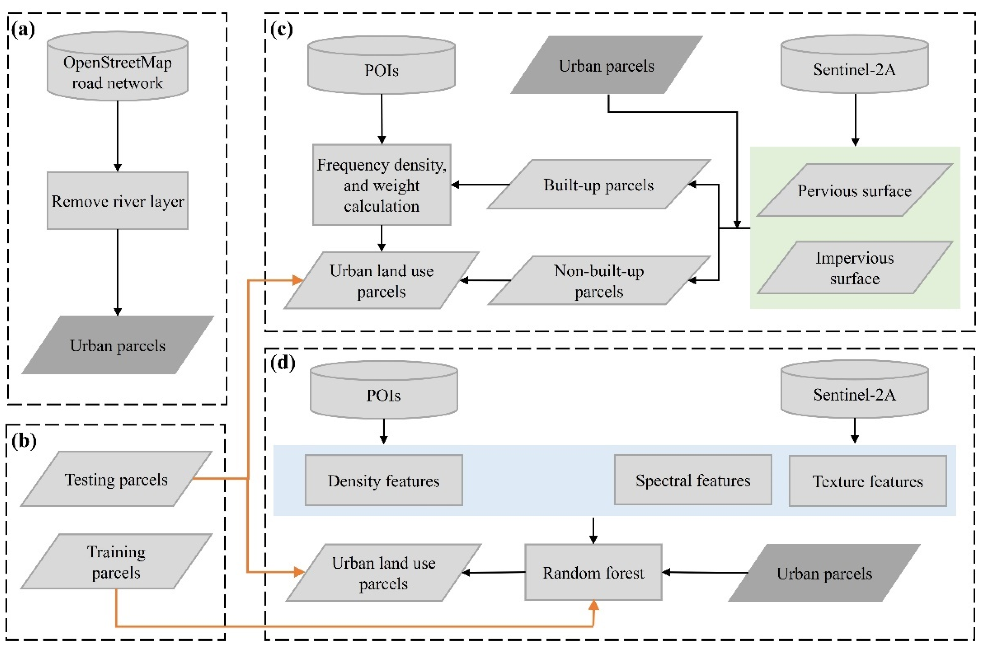
3.3.1. Urban Parcel Generation
3.3.2. Training and Testing Parcel Collection
3.3.3. DI-Based Urban Land Use Mapping
3.3.4. FI-Based Urban Land Use Mapping
3.3.5. Analysis of the DI-Based and FI-Based Classification
4. Results
4.1. Quantitative Performance of DI-Based and FI-Based Urban Land Use Mapping
4.2. Qualitative Performance of DI-Based and FI-Based Urban Land Use Mapping
5. Discussion
5.1. Summary of the Advantages and Disadvantages of the Two Methods
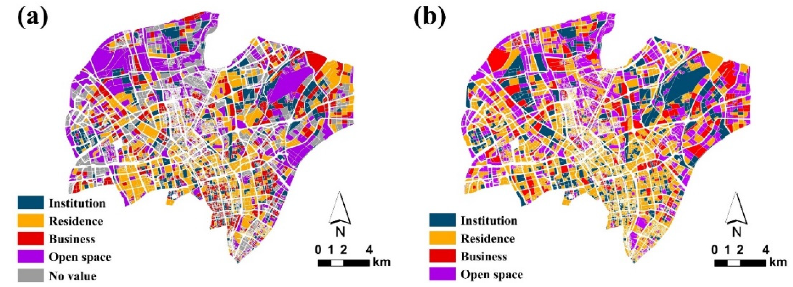
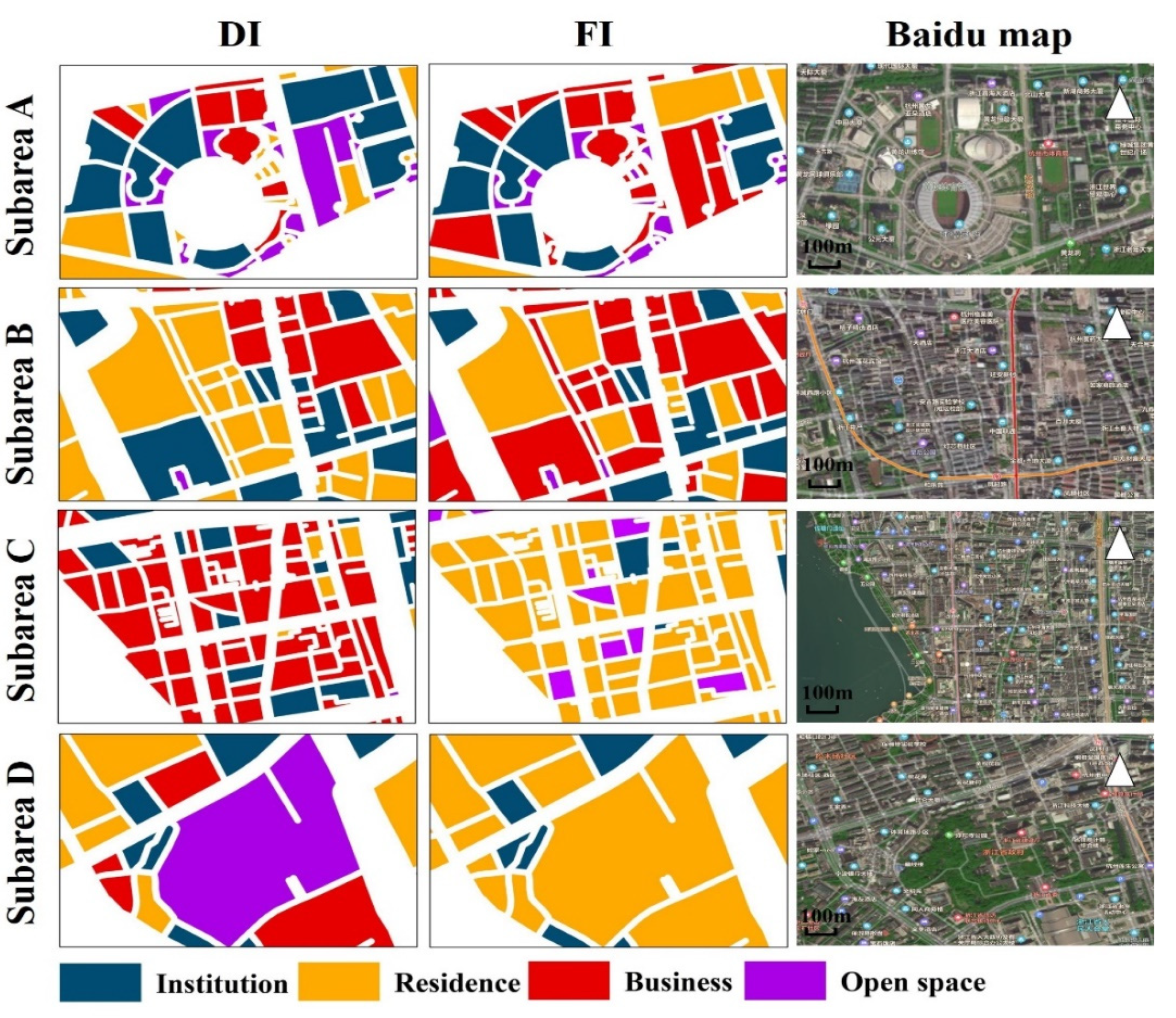
- DI-based urban land use mapping is easy to implement, avoids feature integration, and accompanies conflicting issues. However, it depends largely on the quality and quantity of the GBD in each urban parcel (it depended on POI data in our case study) which might cause the missing value and misclassification for some urban parcels (Figure 7 and Figure 8). For example, Zhao et al. [28] indicated that inaccurate POI will produce incorrect labels, as the classification results are directly generated from POI. Furthermore, the classes used in this paper might not match well with the POI classes considering that DI-based classification is based on labeling parcels based on POI. Reclassifying POI classes according to the nomenclature of land use types can result in some uncertainties of urban land use classification. For example, certain POI could be associated with more than one type of urban land use;
- The FI-based land use mapping enables the mixture of features from RS and GBD, however, the implementation has challenges due to the modality gap [20,32] between the RS and GBD, such as the spatial data quality, technical format, and data structure. Moreover, both feature selection and feature integration in the FI-based classification can contribute to different mapping results. In this study, spectral features and textural features derived from the Sentinel-2 image were integrated with the density features derived from POI for mapping urban land use (Table 3). Accordingly, these features have multiple backgrounds and thus can have various understandings of urban land use mapping, leading to different classification results [65]. The performance of the FI-based classification is probably related to the complexity of urban parcels. To be more specific, a single urban parcel can comprise different urban land uses, such as office buildings, residential buildings, and shopping centers. Therefore, the differences in features among urban parcels might be hard to distinguish.
5.2. The Improved Method for Urban Land Use Mapping
6. Conclusions
Supplementary Materials
Author Contributions
Funding
Acknowledgments
Conflicts of Interest
References
- Gong, P.; Li, X.; Zhang, W. 40-Year (1978–2017) human settlement changes in China reflected by impervious surfaces from satellite remote sensing. Sci. Bull. 2019, 64, 756–763. [Google Scholar] [CrossRef] [Green Version]
- Zhu, Z.; Zhou, Y.; Seto, K.C.; Stokes, E.C.; Deng, C.; Pickett, S.T.A.; Taubenböck, H. Understanding an urbanizing planet: Strategic directions for remote sensing. Remote Sens. Environ. 2019, 228, 164–182. [Google Scholar] [CrossRef]
- Liu, X.; Hu, G.; Chen, Y.; Li, X.; Xu, X.; Li, S.; Pei, F.; Wang, S. High-resolution multi-temporal mapping of global urban land using Landsat images based on the Google Earth Engine Platform. Remote Sens. Environ. 2018, 209, 227–239. [Google Scholar] [CrossRef]
- Reba, M.; Seto, K.C. A systematic review and assessment of algorithms to detect, characterize, and monitor urban land change. Remote Sens. Environ. 2020, 242, 111739. [Google Scholar] [CrossRef]
- Qi, L.; Li, J.; Wang, Y.; Gao, X. Urban observation: Integration of remote sensing and social media data. IEEE J. Select. Top. Appl. Earth Observat. Remote Sens. 2019, 1–13. [Google Scholar] [CrossRef]
- Li, J.; He, Z.; Plaza, J.; Li, S.; Chen, J.; Wu, H.; Wang, Y.; Liu, Y. Social media: New perspectives to improve remote sensing for emergency response. Proc. IEEE 2017, 105, 1900–1912. [Google Scholar] [CrossRef]
- Cai, J.; Huang, B.; Song, Y. Using multi-source geospatial big data to identify the structure of polycentric cities. Remote Sens. Environ. 2017, 202, 210–221. [Google Scholar] [CrossRef]
- Kitchin, R.; McArdle, G. What makes Big Data, Big Data? Exploring the ontological characteristics of 26 datasets. Big Data Soc. 2016, 3, 205395171663113. [Google Scholar] [CrossRef]
- Li, S.; Dragicevic, S.; Castro, F.A.; Sester, M.; Winter, S.; Coltekin, A.; Pettit, C.; Jiang, B.; Haworth, J.; Stein, A.; et al. Geospatial big data handling theory and methods: A review and research challenges. ISPRS J. Photogramm. Remote Sens. 2016, 115, 119–133. [Google Scholar] [CrossRef] [Green Version]
- Ratti, C.; Frenchman, D.; Pulselli, R.M.; Williams, S. Mobile landscapes: Using location data from cell phones for urban analysis. Environ. Plann. B Plann. Des. 2016, 33, 727–748. [Google Scholar] [CrossRef]
- Wu, L.; Cheng, X.; Kang, C.; Zhu, D.; Huang, Z.; Liu, Y. A framework for mixed-use decomposition based on temporal activity signatures extracted from big geo-data. Int. J. Digit. Earth 2020, 13, 708–726. [Google Scholar] [CrossRef]
- Andrade, R.; Alves, A.; Bento, C. POI mining for land use classification: A case study. ISPRS Int. J. Geo-Inf. 2020, 9, 493. [Google Scholar] [CrossRef]
- Ilieva, R.T.; McPhearson, T. Social-media data for urban sustainability. Nat. Sustain. 2018, 1, 553–565. [Google Scholar] [CrossRef]
- Yammine, S.Z.; Jarreau, P.B.; Liu, C.; Coe, I.R. Social media for social change in science. Science 2018, 360, 163. [Google Scholar]
- Ye, X.; Huang, Q.; Li, W. Integrating big social data, computing and modeling for spatial social science. Cartogr. Geogr. Inf. Sci. 2016, 43, 377–378. [Google Scholar] [CrossRef] [Green Version]
- Niu, N.; Liu, X.; Jin, H.; Ye, X.; Liu, Y.; Li, X.; Chen, Y.; Li, S. Integrating multi-source big data to infer building functions. Int. J. Geogr. Inf. Sci. 2017, 31, 1871–1890. [Google Scholar] [CrossRef]
- Srivastava, S.; Vargas Muñoz, J.E.; Lobry, S.; Tuia, D. Fine-grained landuse characterization using ground-based pictures: A deep learning solution based on globally available data. Int. J. Geogr. Inf. Sci. 2018, 34, 1117–1136. [Google Scholar] [CrossRef]
- Krylov, V.; Kenny, E.; Dahyot, R. Automatic discovery and geotagging of objects from street view imagery. Remote Sens. 2018, 10, 661. [Google Scholar] [CrossRef] [Green Version]
- Cadavid Restrepo, A.M.; Yang, Y.R.; Hamm, N.A.S.; Gray, D.J.; Barnes, T.S.; Williams, G.M.; Soares Magalhaes, R.J.; McManus, D.P.; Guo, D.; Clements, A.C.A. Land cover change during a period of extensive landscape restoration in Ningxia Hui Autonomous Region, China. Sci. Total Environ. 2017, 598, 669–679. [Google Scholar] [CrossRef]
- Liu, Y.; Liu, X.; Gao, S.; Gong, L.; Kang, C.; Zhi, Y.; Chi, G.; Shi, L. Social sensing: A new approach to understanding our socioeconomic environments. Ann. Assoc. Am. Geogr. 2015, 105, 512–530. [Google Scholar] [CrossRef]
- Li, J.; Benediktsson, J.A.; Zhang, B.; Yang, T.; Plaza, A. Spatial technology and social media in remote sensing: Challenges and opportunities. Proc. IEEE 2017, 105, 1583–1585. [Google Scholar] [CrossRef] [Green Version]
- Sarmin, N.S.; Ismail, M.H. A review of potentialities and challenges of integrating remote sensing and GIS with socioeconomic data. PJSRR 2016, 2, 129–141. [Google Scholar]
- Dong, J.; Metternicht, G.; Hostert, P.; Fensholt, R.; Chowdhury, R.R. Remote sensing and geospatial technologies in support of a normative land system science: Status and prospects. Curr. Opin. Environ. Sustain. 2019, 38, 44–52. [Google Scholar] [CrossRef]
- Xiong, G.; Cao, X.; Hamm, N.A.S.; Lin, T.; Zhang, G.; Chen, B. Unbalanced development characteristics and driving mechanisms of regional urban spatial form: A case study of Jiangsu Province, China. Sustainability 2021, 13, 3121. [Google Scholar] [CrossRef]
- Zhang, X.; Du, S.; Zheng, Z. Heuristic sample learning for complex urban scenes: Application to urban functional-zone mapping with VHR images and POI data. ISPRS J. Photogramm. Remote Sens. 2020, 161, 1–12. [Google Scholar] [CrossRef]
- Goffi, A.; Bordogna, G.; Stroppiana, D.; Boschetti, M.; Brivio, P.A. Knowledge and data-driven mapping of environmental status indicators from remote sensing and VGI. Remote Sens. 2020, 12, 495. [Google Scholar] [CrossRef] [Green Version]
- Zhang, Y.; Li, Q.; Tu, W.; Mai, K.; Yao, Y.; Chen, Y. Functional urban land use recognition integrating multi-source geospatial data and cross-correlations. Comput. Environ. Urban Syst. 2019, 78, 101374. [Google Scholar] [CrossRef]
- Zhao, W.; Bo, Y.; Chen, J.; Tiede, D.; Blaschke, T.; Emery, W.J. Exploring semantic elements for urban scene recognition: Deep integration of high-resolution imagery and OpenStreetMap (OSM). ISPRS J. Photogramm. Remote Sens. 2019, 151, 237–250. [Google Scholar] [CrossRef]
- Shi, Y.; Qi, Z.; Liu, X.; Niu, N.; Zhang, H. Urban land use and land cover classification using multisource remote sensing images and social media data. Remote Sens. 2019, 11, 2719. [Google Scholar] [CrossRef] [Green Version]
- Liu, X.; He, J.; Yao, Y.; Zhang, J.; Liang, H.; Wang, H.; Hong, Y. Classifying urban land use by integrating remote sensing and social media data. Int. J. Geogr. Inf. Sci. 2017, 31, 1675–1696. [Google Scholar] [CrossRef]
- Jia, Y.; Ge, Y.; Ling, F.; Guo, X.; Wang, J.; Wang, L.; Chen, Y.; Li, X. Urban land use mapping by combining remote sensing imagery and mobile phone positioning data. Remote Sens. 2018, 10, 446. [Google Scholar] [CrossRef] [Green Version]
- Cao, R.; Tu, W.; Yang, C.; Li, Q.; Qiu, G. Deep learning-based remote and social sensing data fusion for urban region function recognition. ISPRS J. Photogramm. Remote Sens. 2020, 163, 82–97. [Google Scholar] [CrossRef]
- Chang, C.; Ye, Z.; Huang, Q.; Wang, C. An integrative method for mapping urban land use change using “geo-sensor” data. In Proceedings of the 1st International ACM SIGSPATIAL Workshop on Smart Cities and Urban Analytics, UrbanGIS’15, Bellevue, WA, USA, 3–6 November 2015; pp. 47–54. [Google Scholar]
- Song, J.; Lin, T.; Li, X.; Prishchepov, A.V. Mapping urban functional zones by integrating very high spatial resolution remote sensing imagery and points of interest: A case study of Xiamen, China. Remote Sens. 2018, 10, 1737. [Google Scholar] [CrossRef] [Green Version]
- Tu, W.; Hu, Z.; Li, L.; Cao, J.; Jiang, J.; Li, Q.; Li, Q. Portraying urban functional zones by coupling remote sensing imagery and human sensing data. Remote Sens. 2018, 10, 141. [Google Scholar] [CrossRef] [Green Version]
- Xu, S.; Qing, L.; Han, L.; Liu, M.; Peng, Y.; Shen, L. A new remote sensing images and point-of-interest fused (RPF) model for sensing urban functional regions. Remote Sens. 2020, 12, 1032. [Google Scholar] [CrossRef] [Green Version]
- Zhang, Y.; Li, Q.; Huang, H.; Wu, W.; Du, X.; Wang, H. The combined use of remote sensing and social sensing data in fine-grained urban land use mapping: A case study in Beijing, China. Remote Sens. 2017, 9, 865. [Google Scholar] [CrossRef] [Green Version]
- Li, D.; Lu, D.; Wu, M.; Shao, X.; Wei, J. Examining land cover and greenness dynamics in Hangzhou bay in 1985–2016 using Landsat time-series data. Remote Sens. 2017, 10, 32. [Google Scholar] [CrossRef] [Green Version]
- Mao, W.; Lu, D.; Hou, L.; Liu, X.; Yue, W. Comparison of machine-learning methods for urban land-use mapping in Hangzhou City, China. Remote Sens. 2020, 12, 2817. [Google Scholar] [CrossRef]
- Drusch, M.; Del Bello, U.; Carlier, S.; Colin, O.; Fernandez, V.; Gascon, F.; Hoersch, B.; Isola, C.; Laberinti, P.; Martimort, P.; et al. Sentinel-2: ESA’s optical high-resolution mission for GMES operational services. Remote Sens. Environ. 2012, 120, 25–36. [Google Scholar] [CrossRef]
- Zhu, Z.; Wang, S.; Woodcock, C.E. Improvement and expansion of the Fmask algorithm: Cloud, cloud shadow, and snow detection for Landsats 4–7, 8, and Sentinel 2 images. Remote Sens. Environ. 2015, 159, 269–277. [Google Scholar] [CrossRef]
- Adiri, Z.; Lhissou, R.; El Harti, A.; Jellouli, A.; Chakouri, M. Recent advances in the use of public domain satellite imagery for mineral exploration: A review of Landsat-8 and Sentinel-2 applications. Ore Geol. Rev. 2020, 117, 103332. [Google Scholar] [CrossRef]
- Weiss, D.J.; Nelson, A.; Gibson, H.S.; Temperley, W.; Peedell, S.; Lieber, A.; Hancher, M.; Poyart, E.; Belchior, S.; Fullman, N.; et al. A global map of travel time to cities to assess inequalities in accessibility in 2015. Nature 2018, 553, 333–336. [Google Scholar] [CrossRef] [PubMed]
- Helbich, M.; Amelunxen, C.; Neis, P.; Zipf, A. Comparative spatial analysis of positional accuracy of OpenStreetMap and proprietary Geodata. In Proceedings of the GI_Forum 2012: Geovisualization, Society and Learning, Salzburg, Austria, 3–6 July 2012; pp. 4–6. [Google Scholar]
- Liu, D.; Chen, N.; Zhang, X.; Wang, C.; Du, W. Annual large-scale urban land mapping based on Landsat time series in Google Earth Engine and OpenStreetMap data: A case study in the middle Yangtze River basin. ISPRS J. Photogramm. Remote Sens. 2020, 159, 337–351. [Google Scholar] [CrossRef]
- Wan, T.; Lu, H.; Lu, Q.; Luo, N. Classification of high-resolution remote-sensing image using OpenStreetMap information. IEEE Geosci. Remote Sens. Lett. 2017, 14, 2305–2309. [Google Scholar] [CrossRef]
- Liu, X.; Long, Y. Automated identification and characterization of parcels with OpenStreetMap and points of interest. Environ. Plann. B 2015, 43, 498–510. [Google Scholar] [CrossRef]
- Rozenfeld, H.D.; Rybski, D.; Gabaix, X.; Makse, H.A. The area and population of cities: New insights from a different perspective on cities. Am. Econ. Rev. 2011, 101, 2205–2225. [Google Scholar] [CrossRef] [Green Version]
- Ministry of Housing and Urban-Rural Development (MoHURD). Code for Design of Urban Road Engineering CJJ37; China Architecture & Building Press: Beijing, China, 2012. [Google Scholar]
- Kang, J.; Körner, M.; Wang, Y.; Taubenböck, H.; Zhu, X.X. Building instance classification using street view images. ISPRS J. Photogramm. Remote Sens. 2018, 145, 44–59. [Google Scholar] [CrossRef]
- Hoffmann, E.J.; Wang, Y.; Werner, M.; Kang, J.; Zhu, X.X. Model fusion for building type classification from aerial and street view images. Remote Sens. 2019, 11, 1259. [Google Scholar] [CrossRef] [Green Version]
- Gong, P.; Chen, B.; Li, X.; Liu, H.; Wang, J.; Bai, Y.; Chen, J.; Chen, X.; Fang, L.; Feng, S.; et al. Mapping essential urban land use categories in China (EULUC-China): Preliminary results for 2018. Sci. Bull. 2020, 65, 182–187. [Google Scholar] [CrossRef] [Green Version]
- Stehman, S.V.; Foody, G.M. Key issues in rigorous accuracy assessment of land cover products. Remote Sens. Environ. 2019, 231, 111199. [Google Scholar] [CrossRef]
- Weng, Q. Remote sensing of impervious surfaces in the urban areas: Requirements, methods, and trends. Remote Sens. Environ. 2012, 117, 34–49. [Google Scholar] [CrossRef]
- Zhao, W.; Li, Q.; Li, B. Extracting hierarchical landmarks from urban POI data. J. Remote Sens. 2011, 15, 973–988. [Google Scholar]
- Puissant, A.; Hirsch, J.; Weber, C. The utility of texture analysis to improve per-pixel classification for high to very high spatial resolution imagery. Int. J. Remote Sens. 2006, 26, 733–745. [Google Scholar] [CrossRef]
- Lu, D.; Weng, Q. Use of impervious surface in urban land-use classification. Remote Sens. Environ. 2006, 102, 146–160. [Google Scholar] [CrossRef]
- Carlson, T.N.; Ripley, D.A. On the relation between NDVI, fractional vegetation cover, and leaf area index. Remote Sens. Environ. 1997, 62, 241–252. [Google Scholar] [CrossRef]
- Heiden, U.; Segl, K.; Roessner, S.; Kaufmann, H. Determination of robust spectral features for identification of urban surface materials in hyperspectral remote sensing data. Remote Sens. Environ. 2007, 111, 537–552. [Google Scholar] [CrossRef] [Green Version]
- Deng, J.; Huang, Y.; Chen, B.; Tong, C.; Liu, P.; Wang, H.; Hong, Y. A methodology to monitor urban expansion and green space change using a time series of multi-sensor SPOT and sentinel-2A images. Remote Sens. 2019, 11, 1230. [Google Scholar] [CrossRef] [Green Version]
- Foody, G.M. Status of land cover classification accuracy assessment. Remote Sens. Environ. 2002, 80, 185–201. [Google Scholar] [CrossRef]
- Card, D.H. Using known map category marginal frequencies to improve estimates of thematic map accuracy. Photogramm. Eng. Remote Sens. 1982, 48, 431–439. [Google Scholar]
- Olofsson, P.; Foody, G.M.; Herold, M.; Stehman, S.V.; Woodcock, C.E.; Wulder, M.A. Good practices for estimating area and assessing accuracy of land change. Remote Sens. Environ. 2014, 148, 42–57. [Google Scholar] [CrossRef]
- Yu, B.; Lian, T.; Huang, Y.; Yao, S.; Ye, X.; Chen, Z.; Yang, C.; Wu, J. Integration of nighttime light remote sensing images and taxi GPS tracking data for population surface enhancement. Int. J. Geogr. Inf. Sci. 2019, 33, 687–706. [Google Scholar] [CrossRef]
- Su, M.; Guo, R.; Chen, B.; Hong, W.; Wang, J.; Feng, Y.; Xu, B. Sampling strategy for detailed urban land use classification: A systematic analysis in Shenzhen. Remote Sens. 2020, 12, 1497. [Google Scholar] [CrossRef]
- Johnson, B.A.; Iizuka, K. Integrating OpenStreetMap crowdsourced data and Landsat time-series imagery for rapid land use/land cover (LULC) mapping: Case study of the Laguna de Bay area of the Philippines. Appl. Geogr. 2016, 67, 140–149. [Google Scholar] [CrossRef]
- Hu, T.; Yang, J.; Li, X.; Gong, P. Mapping urban land use by using Landsat images and open social data. Remote Sens. 2016, 8, 151. [Google Scholar] [CrossRef]
- Pan, H.; Tong, X.; Xu, X.; Luo, X.; Jin, Y.; Xie, H.; Li, B. Updating of land cover maps and change analysis using GlobeLand30 product: A case study in Shanghai metropolitan area, China. Remote Sens. 2020, 12, 3147. [Google Scholar] [CrossRef]


| Gaode POI Classification | Urban Land Use Classification |
|---|---|
| Governmental organization | Institution |
| Medical service | |
| Finance and Insurance service | |
| Sports and Recreation | |
| Culture and Education | |
| Daily life service | Residence |
| Commercial house | |
| Commercial service | Business |
| Shopping | |
| Food and Beverages | |
| Enterprises | |
| Accommodation service | |
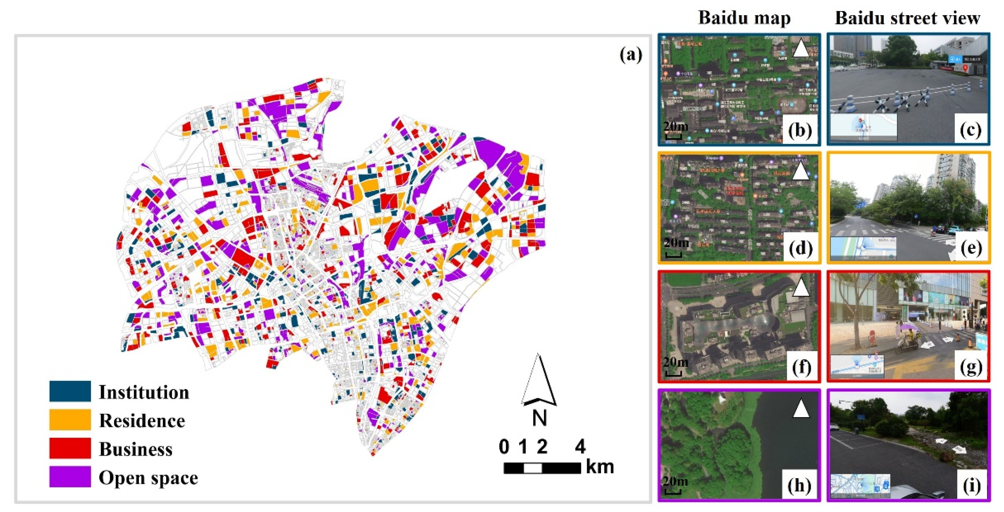
| Tourist attraction | Open space |
| Classes | Road Descriptions | Road Widths (m) | River Descriptions | River Widths (m) |
|---|---|---|---|---|
| Level 1 | Trunk, primary, motorway, railway | 40 | Main rivers | 50 |
| Level 2 | Secondary | 20 | Intermediate rivers | 20 |
| Level 3 | Tertiary, unclassified, residential, service, others | 10 | Small rivers | 10 |
| Feature Types | Indices |
|---|---|
| Spectral features | Enhanced Vegetation Index (EVI), Normal Difference Built-up Index (NDBI), Normal Difference Vegetation Index (NDVI), Normal Difference Water Index (NDWI), mean, standard deviation, kurtosis, skewness |
| Textural features | Angular second moment, contrast, dissimilarity, and entropy |
| Density features | Minimum, maximum, range, sum, mean and standard deviation |
| Map Category | ||||||
|---|---|---|---|---|---|---|
| Class | Pervious | Impervious | Total | PA | OA | |
| True Category | Pervious | 0.240 | 0.018 | 0.258 | 0.928 ± 0.022 | 0.971 ± 0.007 |
| Impervious | 0.010 | 0.732 | 0.742 | 0.986 ± 0.005 | ||
| Total () | 0.250 | 0.750 | 1.000 | |||
| UA | 0.958 ± 0.018 | 0.975 ± 0.008 | ||||
| Map Category | ||||||||
|---|---|---|---|---|---|---|---|---|
| Class | I | R | B | O | Total | PA | OA | |
| True Category | I | 0.071 | 0.029 | 0.042 | 0.014 | 0.156 | 0.453 ± 0.107 | 0.635 ± 0.049 |
| R | 0.015 | 0.326 | 0.072 | 0.008 | 0.421 | 0.774 ± 0.055 | ||
| B | 0.034 | 0.065 | 0.157 | 0.010 | 0.265 | 0.591 ± 0.082 | ||
| O | 0.019 | 0.029 | 0.029 | 0.081 | 0.158 | 0.514 ± 0.102 | ||
| Total () | 0.138 | 0.448 | 0.300 | 0.113 | 1.000 | |||
| UA | 0.512 ± 0.140 | 0.728 ± 0.069 | 0.522 ± 0.095 | 0.714 ± 0.140 | ||||
| Map Category | ||||||||
|---|---|---|---|---|---|---|---|---|
| Class | I | R | B | O | Total | PA | OA | |
| True Category | I | 0.071 | 0.030 | 0.025 | 0.016 | 0.142 | 0.496 ± 0.092 | 0.569 ± 0.041 |
| R | 0.020 | 0.291 | 0.108 | 0.019 | 0.439 | 0.663 ± 0.045 | ||
| B | 0.036 | 0.112 | 0.124 | 0.012 | 0.284 | 0.436 ± 0.062 | ||
| O | 0.008 | 0.028 | 0.015 | 0.084 | 0.135 | 0.620 ± 0.094 | ||
| Total () | 0.135 | 0.462 | 0.272 | 0.130 | 1.000 | |||
| UA | 0.523 ± 0.114 | 0.631 ± 0.059 | 0.453 ± 0.080 | 0.640 ± 0.111 | ||||
Publisher’s Note: MDPI stays neutral with regard to jurisdictional claims in published maps and institutional affiliations. |
© 2021 by the authors. Licensee MDPI, Basel, Switzerland. This article is an open access article distributed under the terms and conditions of the Creative Commons Attribution (CC BY) license (https://creativecommons.org/licenses/by/4.0/).
Share and Cite
Yin, J.; Fu, P.; Hamm, N.A.S.; Li, Z.; You, N.; He, Y.; Cheshmehzangi, A.; Dong, J. Decision-Level and Feature-Level Integration of Remote Sensing and Geospatial Big Data for Urban Land Use Mapping. Remote Sens. 2021, 13, 1579. https://0-doi-org.brum.beds.ac.uk/10.3390/rs13081579
Yin J, Fu P, Hamm NAS, Li Z, You N, He Y, Cheshmehzangi A, Dong J. Decision-Level and Feature-Level Integration of Remote Sensing and Geospatial Big Data for Urban Land Use Mapping. Remote Sensing. 2021; 13(8):1579. https://0-doi-org.brum.beds.ac.uk/10.3390/rs13081579
Chicago/Turabian StyleYin, Jiadi, Ping Fu, Nicholas A. S. Hamm, Zhichao Li, Nanshan You, Yingli He, Ali Cheshmehzangi, and Jinwei Dong. 2021. "Decision-Level and Feature-Level Integration of Remote Sensing and Geospatial Big Data for Urban Land Use Mapping" Remote Sensing 13, no. 8: 1579. https://0-doi-org.brum.beds.ac.uk/10.3390/rs13081579