Land Consumption Monitoring with SAR Data and Multispectral Indices

Abstract

Land consumption is the increase in artificial land cover, which is a major issue for environmental sustainability. In Italy, the Italian Institute for Environmental Protection and Research (ISPRA) and National System for Environmental Protection (SNPA) have the institutional duty to monitor land consumption yearly, through the photointerpretation of high-resolution images. This study intends to develop a methodology in order to produce maps of land consumption, by the use of the semi-automatic classification of multitemporal images, to reduce the effort of photointerpretation in detecting real changes. The developed methodology uses vegetation indices calculated over time series of images and decision rules. Three variants of the methodology were applied to detect the changes that occurred in Italy between the years 2018 and 2019, and the results were validated using ISPRA official data. The results show that the produced maps include large commission errors, but thanks to the developed methodology, the area to be photointerpreted was reduced to 7300 km² (2.4% of Italian surface). The third variant of the methodology provided the highest detection of changes: 70.4% of the changes larger than 100 m² (the pixel size) and over 84.0% of changes above 500 m². Omissions are mainly related to single pixel changes, while larger changes are detected by at least one pixel in most of the cases. In conclusion, the developed methodology can improve the detection of land consumption, focusing photointerpretation work over selected areas detected automatically.

1. Introduction

Soil is a natural resource that plays a fundamental role in providing environmental, social and economic functions. “Soil is generally defined as the top layer of the earth’s crust, formed by mineral particles, organic matter, water, air and living organisms. It is the interface between earth, air and water and hosts most of the biosphere“ [1]. As highlighted by the New Soil Strategy, it “is crucial for fighting climate change, protecting human health, safeguarding biodiversity and ecosystems”. The New Soil Strategy [2] is a European Commission initiative promoted in close coordination and complementarity with other European initiatives [3], such as the EU Biodiversity Strategy for 2030 [4] and Farm to Fork Strategy [5], which will include legally binding targets to protect soil and its degradation.

Land consumption represents one of the main drivers of land degradation [6], and it is the cause of primary ecosystem service loss, such as the capability of food production [7,8] and the fragmentation of habitats [9], particularly when soil sealing occurs.

Soil sealing alters the hydrological cycle and increases the hydraulic hazard in urban areas [10], not allowing water to infiltrate and directly increasing water runoff with significant implications (e.g., reducing the groundwater recharge and soil erosion, and increasing the frequency of flood events).

Land consumption is nominally monitored under the name of Land Take and Soil Sealing at the European scale, by the European Environmental Agency. Employing the CORINE Land Cover data sets in the SOER report [11], the long-term changes over the period 2000–2018 show that the area of artificial surfaces in Europe has changed the most, with an increase of 7.1%.

1.1. Definitions of Land Consumption

Definitions of land consumption have become a relevant issue; sometimes, it is referred to as land take or soil sealing, but rarely in a univocal and homogeneous way. In this work, land consumption is defined as the replacement of non-artificial land cover with artificial land cover related to soil sealing (e.g., construction of buildings and infrastructures, regardless of whether they are 2D or 3D), but it is also used to indicate surfaces modified by reversible consumption processes, such as soil excavation or compaction, where a natural surface has been replaced by artificial material, or a natural material has been removed from its place of origin [12] (e.g., unpaved parking, dumps and quarries), excluding vegetated and green urban areas [13]. This effort of conceptual clarity, proposed in this paper, is a crucial step in order to be aligned with the concept carried on by the new European approach on land monitoring through the EIONET Action Group on Land monitoring in Europe (EAGLE).

Table A1. Relevant definitions related to land cover, land use and land consumption.

Land Consumption (Land Take)	The replacement of a non-artificial land cover to an artificial land cover, both permanent and reversible [13], as explained below. Artificial surfaces that have been changed by, or are under the influence of, human activities resulting in a land consumption process can be sealed or non-sealed [13,64]. We refer to the portion of territory undergoing this process as land consumed.
Permanent Land Consumption (Soil Sealing)	The part of the space that is covered with artificial constructions, such as a building, or surfaces, such as a pavement. It includes buildings, paved roads, railways, airports (paved areas), ports (paved areas), other paved or sealed surfaces, waste dumps and paved greenhouses. It can be considered as Sealed Artificial Surfaces and Constructions. As defined in the Land Cover Component of the Eagle Matrix class 1.1.1 [64].
Reversible Land Consumption	Any process where natural surface material has been replaced by artificial material or where natural material has been removed from, forming a non-impervious and non-built-up surface as stated in the Eagle class 1.1.2 Non-sealed Artificial Surface [64]. It includes soil compaction; excavation; temporary impervious coverage, e.g., unpaved roads, construction sites, courtyards or sports fields; permanent deposits of material; photovoltaic fields; and quarries not yet restored.
Land Cover	The physical and biological cover of the Earth’s surface, including artificial surfaces, agricultural areas, forests, (semi)natural areas, wetlands and water bodies. It is an abstraction of reality as the Earth´s surface is populated with landscape elements. [65]
Land Use	The territory characterized according to its current and future planned functional dimension or socioeconomic purpose (e.g., residential, industrial, commercial, agricultural, forestry and recreational). Land Use is different from Land Cover, dedicated to the description of the surface of the Earth by its (bio)physical characteristics [65].

provides a synthesis of the meaning of terms considered in this work.

1.2. Soil Protection Policy and Actions

In the European framework, several policies are addressed to protect land and reduce degradation, although none of them has a binding legislative function on the planning policies of the different Member States.

Table A2. Relevant initiatives in the framework of soil protection: the objectives they intend to achieve are indicated with the target year.

Strategic Documents and Policy Guidelines	Year	Soil Aspects	Objectives and Targets	Target Year
Thematic strategy on the protection of soil [1]	2006	Prevent further degradation of soil, preserve its functions and restore degraded soil + integrate soil protection into relevant EU policies.	Soil Directive	N/A
Roadmap to a resource efficient Europe (EU) [15]	2011	Reduce soil erosion, increase soil organic matter and promote remedial work on contaminated sites.	Achieve no net land take by 2050.	2020 /2050
Soil Sealing Guidelines [16]	2012	Guidelines explicitly focus on limiting, mitigating and compensating for the effects of soil sealing.		N/A
The Seventh Environment Action Programme (7th EAP) [17]	2013	EU policies help to achieve no net land take by 2050.	Achieve no net land take by 2050.	2050
The 2030 Agenda for Sustainable Development and its 17 Sustainable Development Goals (SDGs), United Nations [18]	2015	The agenda points to 17 Sustainable Development Goals (SDGs), and 169 associated targets on the theme of protection, conservation and sustainable management of natural resources. Goal 15.3 "land degradation neutrality" Goal 11 “Make cities and human settlements inclusive, safe, resilient and sustainable “.	Target 15.3.1: by 2030, achieve a land degradation-neutral world; target 11.3.1: by 2030, the increase in the population should be aligned to the expansion of built-up area; target 11.7: by 2030 to “provide universal access to safe, inclusive and accessible, green and public spaces...".	2030
The European Green Deal [3]	2019	The European Green Deal is a response to tackle climate change growth and environmental degradation and aims at a revision of relevant legislative measures to deliver on the increased climate ambition, following the review of land use and land use change and forestry regulation.
EU biodiversity strategy [4]	2020	The strategy contains specific actions to protect nature and reverse the degradation of ecosystems and aims to prevent the loss of biodiversity and ecosystem services in the EU by 2030; it includes positive implications for a wide number of soil threats and functions.	Legally protect a minimum of 30% of the EU’s land and (sea) area; restore degraded ecosystems by adopting sustainable soil management practices limiting urban sprawl and greening urban and peri-urban areas.	2030
Healthy soils – new EU soil strategy [2]	2020	Update of the current soil strategy to address soil degradation (currently under public consultation), protect soil fertility, reduce erosion and sealing, increase organic matter, identify contaminated sites, restore degraded soils.	Achieve land degradation neutrality by 2030; reduce the rate of land take, urban sprawl and sealing to achieve no net land take by 2050.	2030 and 2050
Caring for soil is caring for life [19]	2020	Proposal to the European Commission to reduce land degradation, conserve and increase soil organic carbon stocks, no net soil sealing, re-use of urban soil for urban development, reduce soil pollution and enhance restoration, prevent erosion, improve soil structure, reduce the EU global footprint on soils, increase soil literacy in society across Member States.	Target 1.1: 50% of degraded land is restored; Target 3.1: switch from 2.4% to no net soil sealing; Target 3.2: the current rate of soil re-use is increased from current 13 to 50% to help meet the EU target of no net land take by 2050; Target 5.1: stop erosion on 30-50% of land with unsustainable erosion rates.	2030
Farm to Fork Strategy [5]	2020	Accelerate our transition to a sustainable food system that should have a neutral or positive environmental impact, help to mitigate climate change, reverse the loss of biodiversity; all actions will contribute to improve soil protection.	Ensuring that the food chain, covering food production, transport, distribution, marketingand consumption have a neutral or positive environmental impact.
Land Degradation Neutrality -Unccd [20]	2015	Halt the ongoing loss of healthy land through degradation.	Reaching the state whereby the amount and quality of land resources necessary to support ecosystem functions and services remains stable or increases within specified temporal and spatial scales and ecosystems.	2030

shows a synthesis of relevant actions for soil protection at the European and global level. In order to support the monitoring of the progress made by the Member States towards the achievement of the objectives, an accurate cartographic reference, with a unique and shared definition of land consumption, is necessary. In particular, the European Seventh Environment Action Programme sets the goal of achieving no net land take by 2050 [14], while the Agenda for Sustainable Development of the United Nations established, through its Sustainable Development Goals (SDGs), two indicators to keep track of land consumption-related issues, such as land degradation and urban growth. While in the SDG 11.3.1, land consumption is an explicit variable, in the SDG 15.3.1, it falls within the broader phenomenon of land degradation, representing a major component of the latter. It is also relevant to mention the new soil strategy (currently under public consultation) that reaffirms the EU target of reducing the rate of land take, urban sprawl and soil sealing to achieve no net land take by 2050.

1.3. Monitoring Land Consumption through Remote Sensing

As illustrated in the previous paragraph, land consumption assessment plays a key role in understanding local pressures and better identifying the drivers behind it, just as it is important to have up-to-date and accurate data available to keep track of land cover changes. Land consumption is becoming better known and spatially localized thanks to the remote sensing monitoring of territory and land cover mapping.

Many initiatives and programs have been undertaken in Europe to obtain information to map land consumption and its changes; among the most relevant is the Copernicus Land Monitoring Service (https://land.copernicus.eu, accessed on 4 March 2021), implemented by the EEA and the JRC, which guarantees full, free and open access to earth observation data [15] for the whole of Europe with repetitiveness and homogeneity [16].

The artificial land cover information can be derived from CORINE Land Cover (CLC) or from High Resolution Layers (HRLs) (https://land.copernicus.eu/pan-european, accessed on 4 March 2021). A third source encompasses Urban Atlas (the local component of Copernicus program), a land cover and land use dataset, which contains a detailed legend on urban characteristics with a Minimum Mapping Unit (MMU) of 0.25 ha. (https://land.copernicus.eu/local/urban-atlas, accessed on 4 March 2021) (

Table 1. Relevant Copernicus data related to land consumption.

Data	CORINE Land Cover	High Resolution Layers	Urban Atlas
Type of information	Land use/Land cover map (44 classes, with 3 level)	Percentage of sealed area	High-resolution Land use/Land cover map (27 classes)
Coverage	EU 39	EU 39	788 FUAS
Minimum Mapping Unit	25 ha and 5 ha (changes)	20 m (pixel), 10 m only 2018	17 urban classes 0.25 ha 10 rural classes 1 ha
Reference year	1990, 2000, 2006, 2012, 2018	2006, 2009, 2012 and 2018 (under validation)	2006, 2012, 2018

).

Nevertheless, there are still some limits to the use of these data for the (detailed) monitoring of land consumption (at national and local levels) with a certain frequency. In fact, they have limits linked to the different classification systems and spatial resolution, but above all, they do not able an annual monitoring of the phenomenon, since CLC and Urban Atlas are updated every six years, while the imperviousness datasets are updated every three years.

In light of these problems, the EU has proposed a new set of products attempting to overcome these difficulties: the realization of a second generation of CLC has recently been launched, with the objective to improve the characteristics of the current national and European data. “CLC+”, for instance, will offer information, with thematic and spatial details, superior to those of the current generation of CLC, and will be based on the Eagle classification system.

The classification system developed in this study is consistent with this scheme; this compliance will be able to support the institutional tasks of ISPRA and the SNPA in their land monitoring activities.

The availability of more data, such as those of the Sentinel-1 and Sentinel-2 missions within the Copernicus program, has offered new and better possibilities to extract land cover information, detect changes from the urban environment [17] and meet the need for the accurate and frequent request of data.

Researchers have made enormous efforts to improve change detection methodologies, and several reviews based on satellite data have been published [18,19,20,21,22,23,24,25,26,27,28,29], only a few of which are specifically addressed to urban detection [20,30].

Many of these studies and reviews stress the difficulty of identifying common guidelines for the choice of the most suitable methodology. Likewise, comparing the accuracy of different techniques is a very hard task for several reasons: it depends, among other things, on the spatial, spectral and temporal resolution of the sensor used and on the objective of the research.

The most commonly used algorithms are based on image differencing; image ratioing [31]; regression analysis; vegetation index differencing; change vector analysis (CVA) [32,33,34]; transformation, as principal component analysis (PCA) [35]; and tasseled cap transformation (KT) machine-learning (such as artificial neural networks, support vector machines and decision trees) [27,36,37], i.e., those using more than one system.

Image differing or ratioing is best suited for change/no-change (binary) information. Most of these techniques are based on the threshold value to discriminate the area changed/not changed; the selection of the best threshold determines the accuracy of the technique used. In order to improve the performance, it is possible to combine different fusion techniques or apply automated threshold algorithms.

Several supervised machine learning techniques are now widely used for urban change detection purposes, and many researchers have highlighted the advantages of these to achieve reliable handle classification [21,30,31,32]. However, the downside of these methods is that it is difficult to find a large number of training areas and to set the user-defined parameters for the algorithm, factors which play an important role in the accuracy of the final results. In addition, machine learning techniques usually require handling considerable quantities of data and complex computational capacity.

One major issue in urban change detection is the discrimination of the spectral difference between the bare soil and urban area. In this context, during harvesting time, herbaceous vegetation (crops) could also be confused with urban areas. Change detection methods that exploit time series of satellites images and the specific characteristics of different sensors, could provide reliable information for solving these difficulties. The combined use of optical and radar data, for example, has produced satisfactory results: the former could provide spectral reflectance and the phenological characteristics of the vegetation, useful to discriminate soil sealing from natural vegetation; the latter offer the possibility to analyze the different behavior of urban surfaces with respect to scattering or polarization to obtain information on a built-up area. In addition, radar collects data in all weather conditions (and fills the gap in cloudy regions), a key feature when studying large areas with a cloudy cover for a part of the year; it should be considered, however, that radar images present speckle noise, an important element for the accuracy of classification processes (https://sentinel.esa.int/web/sentinel/user-guides/sentinel-1-sar, accessed on 4 March 2021).

Ban et al. [38] used both of these two sensors for urban land cover mapping in an object-based classification method; Pasaresi et al. [39] used fused data for improving the results of urban settlement map; Jan Haas and Yifang Ban [40] segmented the combination of Sentinel SAR and MSI image stacking to classify the Zürich metropolitan area using the SVM algorithm; Goldbatt et al. [41] mapped built up changes in Ho Chi Minh City, Vietnam; Celik and Sun et al. [42,43] performed extracted urban land cover information from Sentinel-1A SAR data and Sentinel-2 MSI based on Google Earth Engine. Iannelli and Gamba [44] applied the Urban Extractor (UEXT) algorithm to detect the urban extraction of Rio de Janeiro and Beijing, showing the results using Sentinel-1 and Sentinel-2. The analysis carried out shows that much progress has been made to analyze land cover changes, and no algorithm can be considered suitable for all change detection applications.

This research aims to develop an innovative methodology for monitoring land consumption on a yearly basis, in support of the monitoring land consumption activities performed by ISPRA-SNPA [45] for the whole Italian territory, as institutionally mandated by Act 132/2016 (establishment SNPA, National System for the Protection of the Environment). The current methodology includes a photointerpretation phase that requires significant efforts in terms of time and human resources for the definition and verification of areas subjected to land cover changes.

The study of a surface as extensive as Italy, through remote sensing data, leads to a number of issues that need to be addressed: inhomogeneity of the territory with different morphologic, vegetation and climatic characteristics; the greater spectral difference that occurs over large areas and the complexity of landscape, as well as the enormous amount of data to be managed. Furthermore, the design requirements defined by ISPRA impose an annual update frequency and the achievement of very high accuracy values (the current cartography reaches 99.7% global accuracy [45]).

In order to overcome these issues, this study developed a hybrid method that allows flexibility, exploits the advantages offered by the GEE platform—able to handle a huge amount of data—and it is unsupervised; therefore, it does not need training samples. A decision rules process was developed, in which each rule aimed to extract specific information from the surface according to the data used; the results are a series of masks containing a part of urban cover.

In addition, Sentinel-1 and Sentinel-2 (multispectral optical and SAR data) were both investigated to overcome the difficulties represented by multispectral data due to the similarity of the spectral signature of some features, through Sentinel 1 and, at the same time, to understand the potential of the integration of these data in the urban field. There are several studies that have proved an increase in accuracy using fusion methods for land cover classification and change detection analysis [40,46]; however, not many studies have highlighted the capability of the combined use of Sentinels 1 and 2 to extract built up changes.

2. Materials and Methods

The methodology presented in this study uses Sentinel-1 GRD and Sentinel-2 images to automatically detect land cover changes caused by land consumption.

The methodology is based on the following assumptions, as well as on the observation of test areas and the literature:

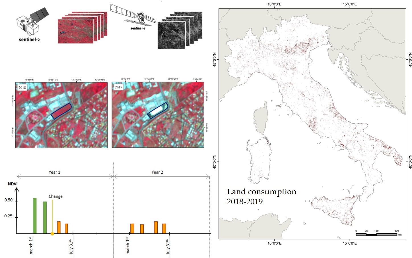
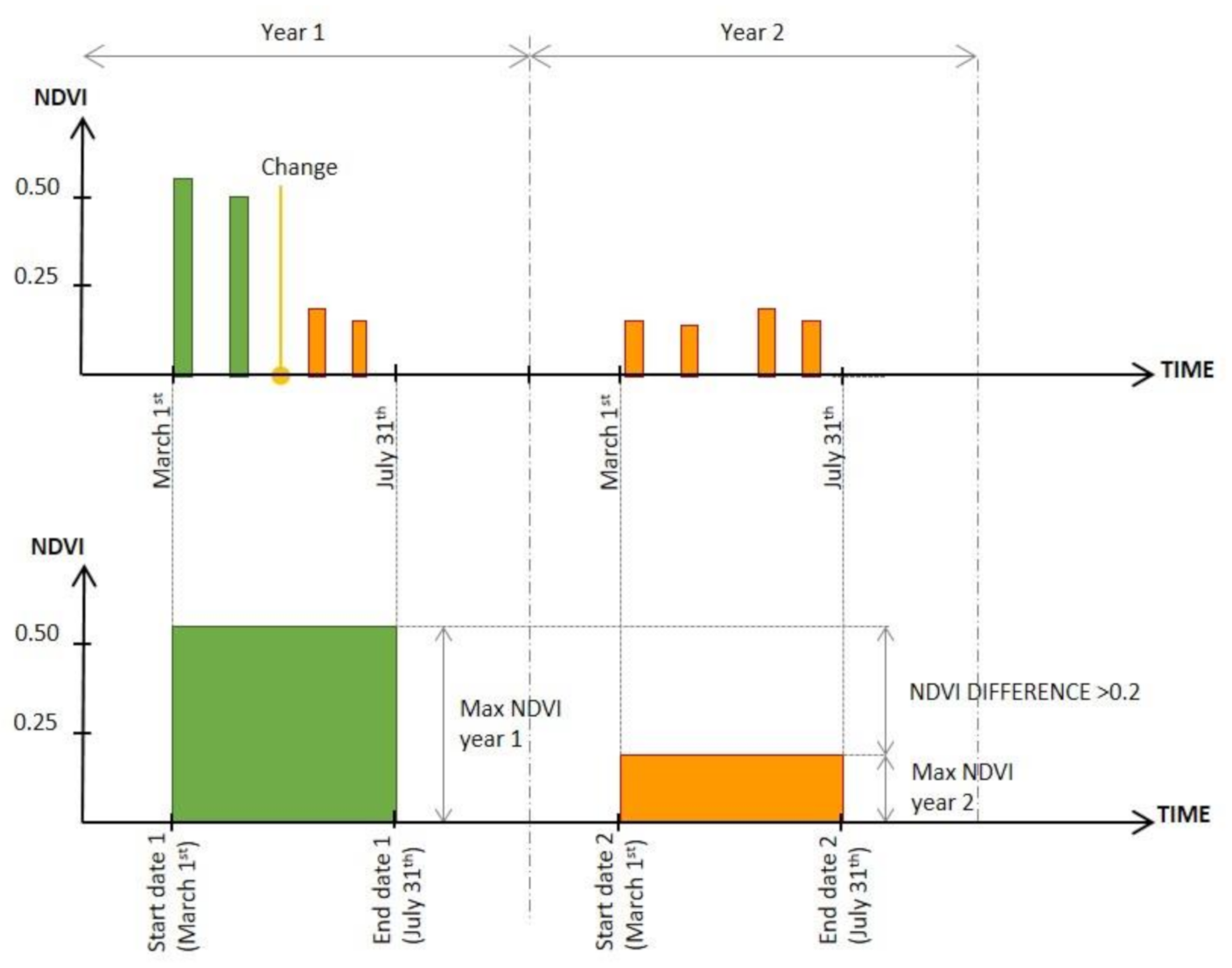
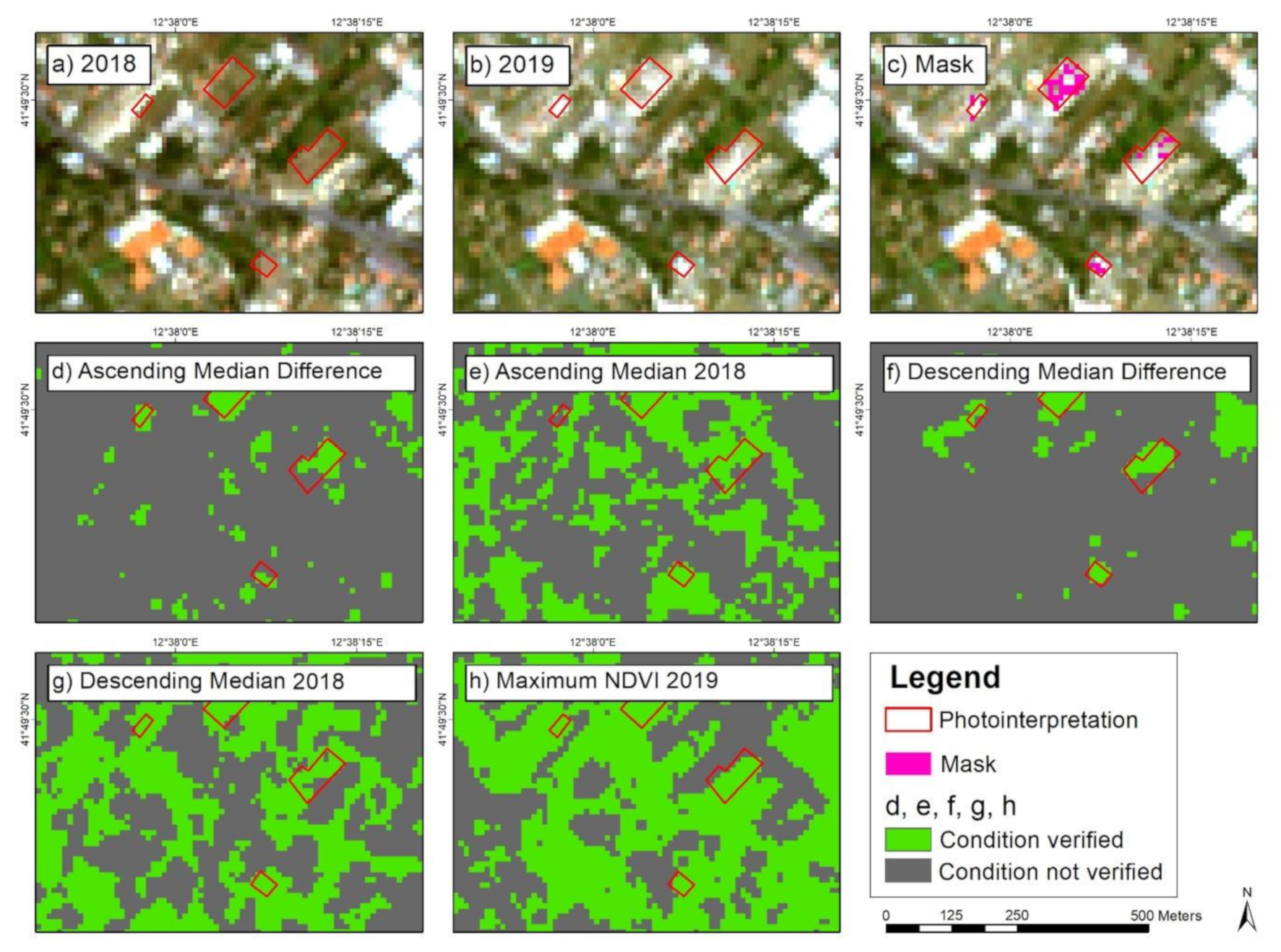
• Land consumption can follow the removal of vegetation cover, if present before the change, and, therefore, causes a decrease in vegetation indices, such as NDVI.
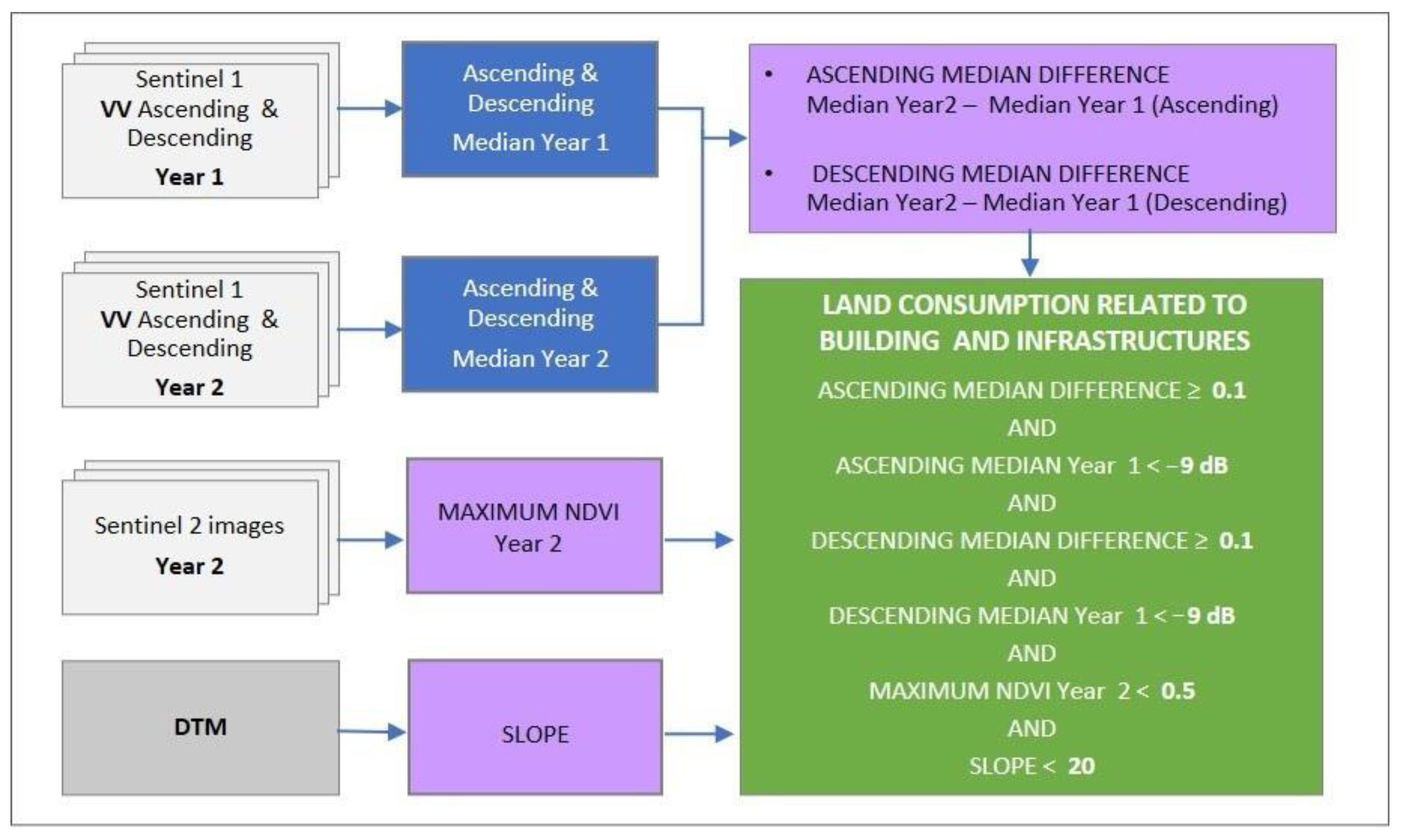
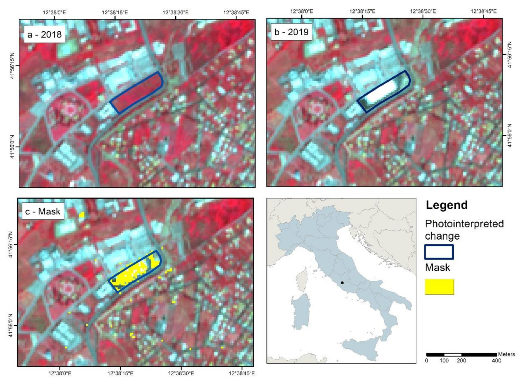
• Built-up areas, such as buildings, infrastructures, or even construction sites, are characterized by high backscattering values, due to multiple reflections or the double-bounce effect [47]. Therefore, land consumption can increase the backscatter if the land cover is characterized by low or intermediate roughness, such as low-vegetation and bare soils before changing.
• Land consumption can be detected if at least one of the above assumptions is verified.

Based on these assumptions, a fully automatic workflow was developed (Figure 1) using multitemporal acquisition of Sentinel-1 GRD and Sentienel-2 images, in order to detect changes that occurred between 2018 and 2019 in the study area of Italy. Sentinel-1 imagery allows us to calculate the backscatter in the polarizations VV and VH, which are influenced by several factors, such as the geometry, dielectric properties and roughness of surfaces [48].

Sentinel-2 images allow us to evaluate spectral characteristics of land surface, related to land cover materials. Previous studies, which monitored land consumption related to the removal of vegetation based on the Normalized Difference Vegetation Index (NDVI), were calculated from Sentinel-2 images [13].

NDVI is defined as follows:

$$NDVI=\frac{\left(NIR-Red\right)}{\left(NIR+Red\right)}$$

(1)

NIR is the reflectance in the near infrared band, and Red is the reflectance of the red band. NDVI ranges from −1 (abiotic cover) to +1 (totally vegetated areas). In general, mixed areas of vegetation cover and non-vegetated cover have an NDVI range between 0.1 and 0.9.

Decision rules are defined to estimate changes at a pixel size of 10 m, setting fixed threshold values on composites (e.g., median, maximum and differences) of multitemporal images. This method does not require a training area. A Digital Terrain Model (DTM) was used to calculate the slope and refine the calculation to avoid errors related to the morphology of mountain areas, where identifying changes is harder due to shadows.

It is worth noting that these classifications of changes are intended to be used to support the ISPRA monitoring of land consumption, in order to reduce the time of photointerpretation as well as reducing the area to be manually analyzed.

As the acquisition orbit influences the angle of view of Sentinel-1 images, the ascending and descending orbits are considered separately, to preserve the information related to object configuration and orientation on the ground.

The backscatter of VH polarization can partially improve the detection of low vegetation or crop [49], while the VV polarization can be more sensitive to soil variations [50], although these considerations should be further investigated for buildings and infrastructures.

The methodology was developed on Google Earth Engine (Javascript language program). The same methodology was applied using the QGIS Semi-Automatic Classification Plugin in a DIAS environment (ONDA https://www.onda-dias.eu, accessed on 4 March 2021), in order to test the classification in an environment different from Google Earth Engine. The DIAS environment allows us to directly access the Copernicus imagery archive (European Commission, 2018), avoiding downloading images and providing a server for cloud computing (i.e., 16 Cores 2.3 GHz and 60 GB of RAM). This DIAS experimentation was in the framework of the Habitat Mapping project (by the Italian Institute for Environmental Protection and Research and the Italian Space Agency).

The output classifications were validated through the photointerpretation of very high-resolution images that allowed us to identify real changes.

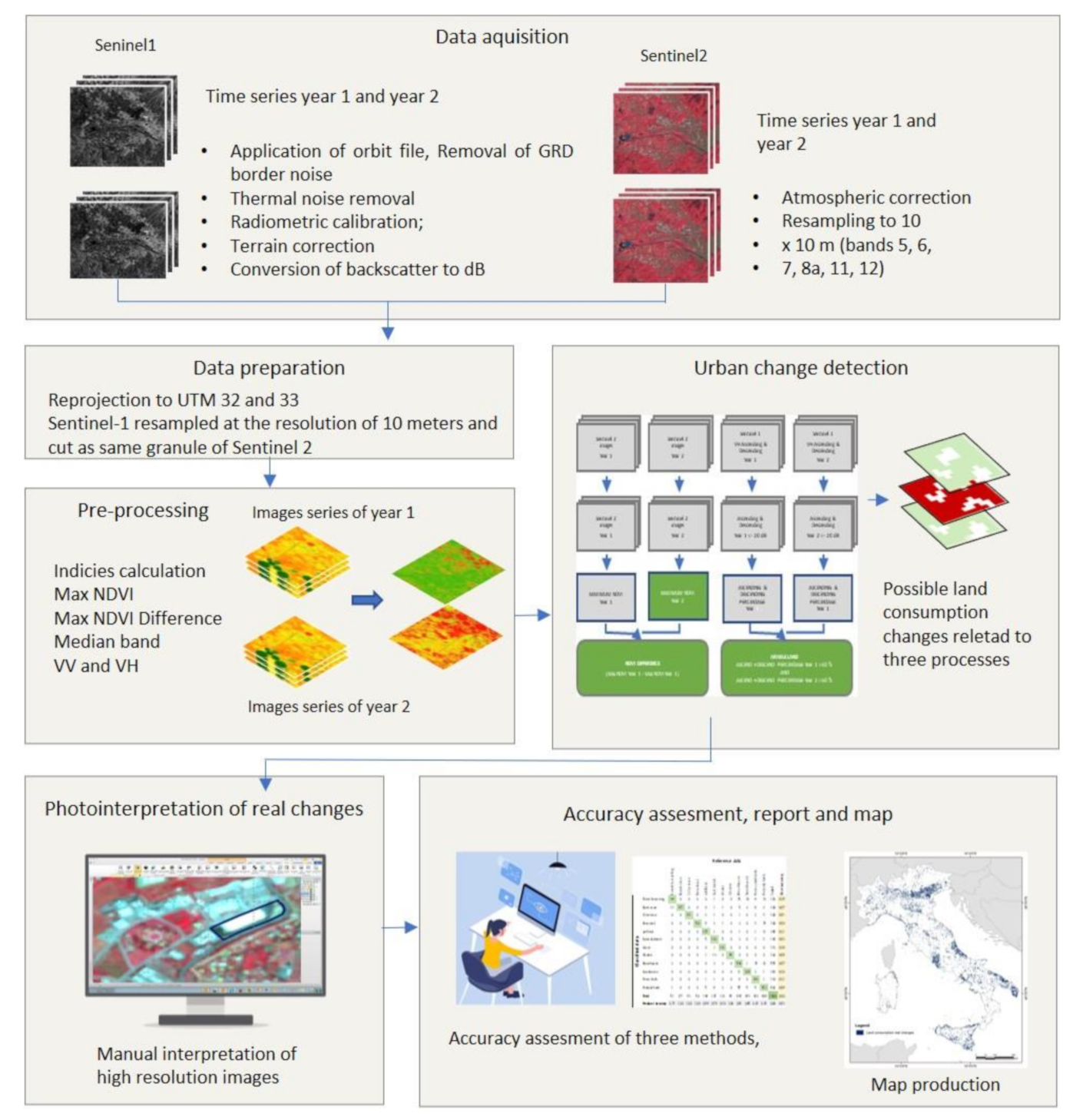
2.1. Images Preprocessing

Using Sentinel-1 GRD and Sentinel-2 images requires a few preprocessing steps in order to obtain the backscatter values and reflectance values. In addition, it is worth noticing that Sentinel-1 GRD and Sentinel-2 grids are not aligned and have different spatial resolutions. Sentinel-1 data were resampled to a spatial resolution of 10 m and aligned to the Sentinel-2 grid to use both images in the same workflow. WGS 84 UTM coordinates were used.

2.1.1. Sentinel-1

Google Earth Engine provides Sentinel-1 GRD images already converted to backscatter values, following the steps described on the website (https://developers.google.com/earth-engine/sentinel1, accessed on 15 February 2021), which are as follows:

• Application of orbit file;
• Removal of GRD border noise (low intensity and invalid data);
• Thermal noise removal to reduce discontinuities between sub-swaths;
• Backscatter intensity calculation using radiometric calibration;
• Terrain correction (orthorectification using the SRTM 30-meter DEM);
• Conversion of backscatter coefficient to dB.

In the DIAS testing, the same methodology was applied to obtain backscatter values from Sentinel-1 GRD images.

2.1.2. Sentinel-2

Sentinel-2 level L1C images were used for 2018 and 2019, as the Google Earth Engine L2A image archive was not complete at the time of the research. A cloud mask was applied to the images with a simple algorithm described on the Google Earth Engine website (https://developers.google.com/earth-engine/datasets/catalog/COPERNICUS_S2, accessed on 4 March 2021). These cloud mask products generally underestimate clouds [51].

Furthermore, the atmospheric disturbance affecting L1C pixels can increase the uncertainty of spectral signatures, so thresholds were selected trying to avoid omission errors in favor of commission errors.

2.2. Detection of Changes Caused by Land Consumption

This methodology of change detection involves the acquisition of multitemporal Sentinel-1 GRD and Sentinel-2 images acquired in 2 years and already preprocessed according to the previous paragraph, in 2018 and 2019. According to the assumptions of this study related to land consumption changes, the following methods were used:

• Sentinel-2 images to calculate NDVI differences in the two years for changes involving the removal of vegetation cover; Sentinel-1 GRD was also used to improve the detection.
• Sentinel-1 GRD to calculate differences in backscatters caused by buildings, infrastructures or construction sites.

For the sake of simplicity, these two methods are explained in two separate paragraphs, even though the model is unique.

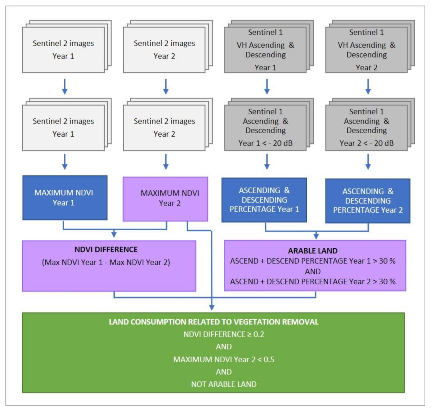
2.2.1. Land Consumption Related to the Removal of Vegetation

The identification of land consumption was conducted by ISPRA through photointerpretation. In order to produce the composites, the acquisition periods between 1st March and 31st July (periods must be the same in the 2 years) were considered. In this period, in Italy, vegetation is at its maximum vegetative growth, guaranteeing the distinction between land consumption and bare soil [13]. In addition, the range is large enough to ensure the availability of cloud-free images.

Since Sentinel-2 images are provided as granules (the minimum partition of the image with size 100 × 100 km²), the steps in the workflow are intended to be performed for each granule. Italy is covered by about 80 granules in the WGS 84 UTM 32 and UTM 33 coordinates.

Three experimental versions were developed and tested (called "approaches"), to assess the benefit of different periods, conditions and thresholds, although the basic approach is the same. In detail, two basic conditions were defined for the detection of changes based on NDVI values, which were used in all three approaches alone or accompanied by other rules:

-

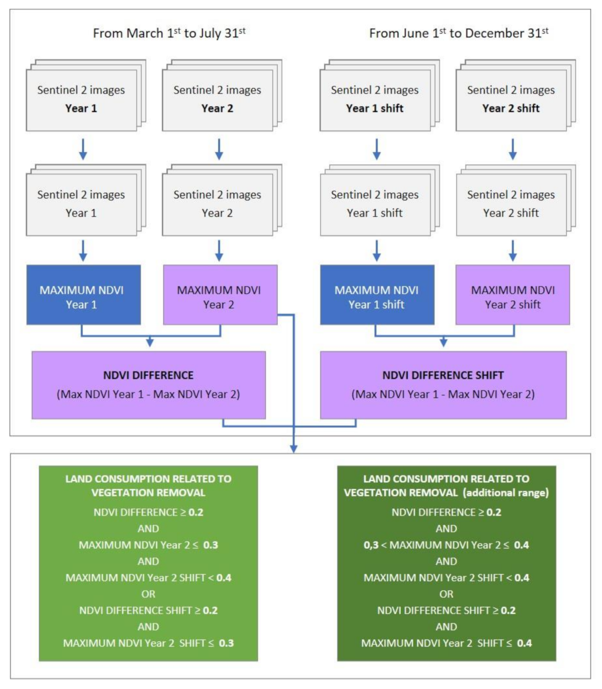
In the first approach, potential changes related to the application of only the two basic conditions are identified for the period between 1st March and 31st July.

-

In the second approach, a third condition is added, in order to filter commission errors related to seasonal variation of vegetation cover in agricultural areas. The reference period is still between 1st March and 31st July.

-

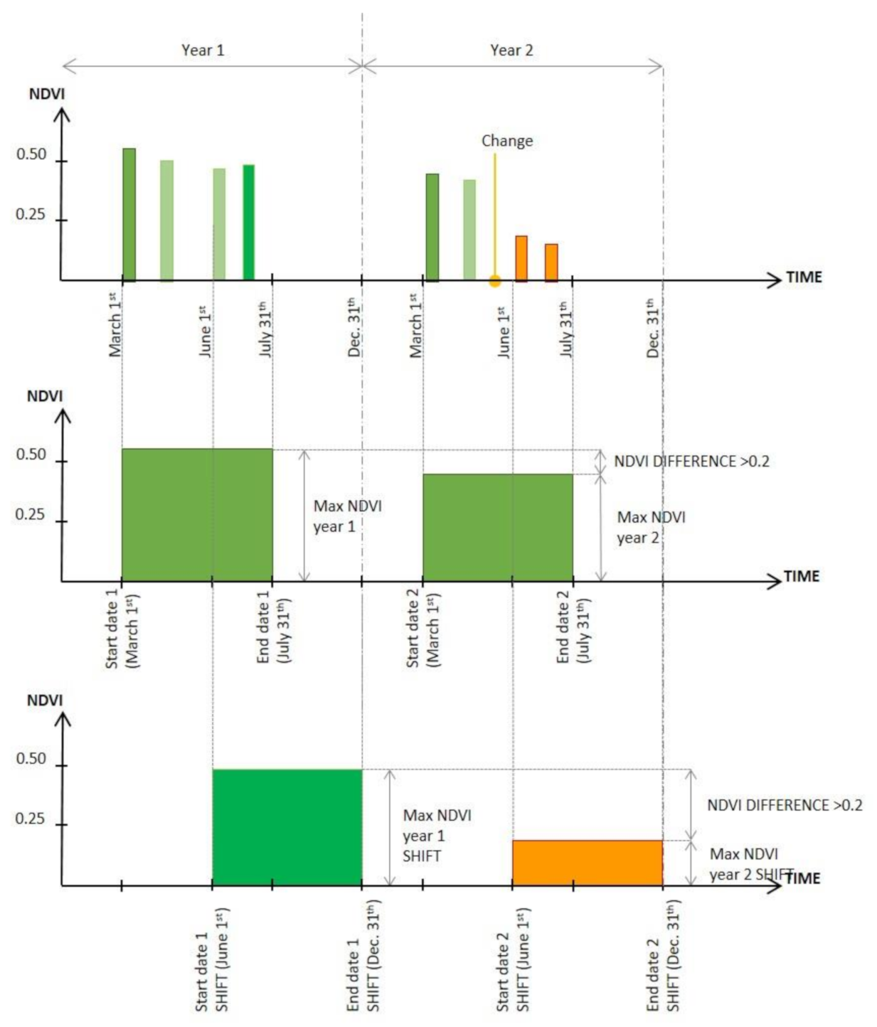
The third approach applies the two basic conditions, varying the reference period to evaluate how the amplitude of the reference period influences the identification of changes. In particular, in addition to the period between 1st March and 31st July, the period from 1st June to 31st December is considered.

The first two approaches are based on thresholds already tested in the bibliography [13,52], while for the third approach, different thresholds were tested to distinguish the most probable changes (relative to more restrictive NDVI values, called “main range”) from less probable ones (relative to a less restrictive “additional range” of NDVI).

The three approaches are detailed below.

The first approach considers that land consumption related to the removal of vegetation had NDVI difference values greater than 0 between the two years and lower NDVI values in the second year. Starting from these considerations, the following two conditions were defined:

NDVI DIFFERENCE ≥ 0.2

(2)

And

MAXIMUM NDVI Year 2 < 0.5

(3)

The first condition (i.e., NDVI DIFFERENCE ≥ 0.2) implies a reduction in vegetation cover, while the second condition (i.e., MAXIMUM NDVI Year 2 < 0.5) verifies the scarcity of vegetation. The threshold values are conservative and derive from the literature and empirical testing [13]. Pixels with NDVI values that meet these conditions have a probable change in land cover caused by land consumption.

Sentinel-2 images were processed according to these steps:

• First, the NDVI was calculated for every image;
• The maximum NDVI value per pixel was calculated for each year, obtaining two rasters (MAXIMUM NDVI rasters);
• These 2 maximum NDVI rasters were used to calculate a raster of NDVI difference between the 2 years (NDVI DIFFERENCE = MAXIMUM NDVI Year 1–MAXIMUM NDVI Year 2);
• Starting from the products of points 2 and 3, a binary mask was created where both conditions are met.

The second approach (Figure 2), in addition to the two conditions defined in the first one, uses Sentinel 1 data to identify agricultural areas. In fact, these areas can be erroneously classified as land consumption due to their spectral behavior (e.g., fallow land cultivated in the first year, and uncultivated in the second year).

An ARABLE LAND filter was defined and tested to identify agricultural land to be excluded from change detection rules as defined in the first approach.

In order to create this raster, Sentinel-1 images with polarization VH were used, according to the following steps:

• Four collections of Sentinel-1 VH images were distinguished by ascending and descending orbit and by the 2 years of acquisition:
  • Ascending year 1;
  • Descending year 1;
  • Ascending year 2;
  • Descending year 2.

The sum of ascending percentage and descending percentage allows us to consider both as viewing geometries, which can cause shadowing and, therefore, affect backscatter values [53]. The images for the 2 years were not used to estimate any difference but to verify the same condition in both years; this could fail the detection of fallow land that exhibits low backscatter values in 1 year only.

2.

A raster was created for each of the four collections, indicating the number of times the backscatter was <−20 dB for each pixel.

The −20dB value is conservative, as fallow land is characterized by backscatter values lower than −11 dB [54]. This value entails the presence of commission errors (agricultural areas with backscatter values higher than −20 dB), but limits the omission errors that would occur, excluding land consumption associated with low backscatter values from the masks.

Commission errors would be eliminated during the manual digitization of the changes, while omission errors would not be considered during photointerpretation, as it focuses on inspecting the masks of potential changes.

Four rasters were obtained:

• Ascending percentage year 1;
• Descending percentage year 1;
• Ascending percentage year 2;
• Descending percentage year 2.

A raster, ARABLE LAND, was calculated according to the following condition:

(Ascending Percentage Year 1 + Descending Percentage Year 1) > 30%

(4)

And

(Ascending Percentage Year 2 + Descending Percentage Year 2) > 30%

(5)

The ARABLE LAND layer is a binary raster whose pixels have a value of 1 if the above conditions are verified; otherwise, the value equals 0.

The ARABLE LAND binary raster represents the areas that verified the condition in 30% of observations (ascending and descending). The threshold was defined by trial and error. These areas are excluded from the masks of potential change as they could be agricultural areas.

It is worth noting that the scope of this ARABLE LAND layer is not classifying arable land in general but detecting the portion of arable land that can be confused with land consumption due to the temporary removal of vegetation.

In the second approach, ARABLE LAND, it is added to the two previous conditions:

NDVI DIFFERENCE between year 1 and year 2 ≥ 0.2

(6)

And

MAXIMUM NDVI Year 2 < 0.5

(7)

And

ARABLE LAND = 0

(8)

The third condition (i.e., ARABLE LAND = 0) has the purpose to exclude false changes that occurred in arable land.

The third approach considers that the amplitude of the reference period influences the identification of changes. Specifically, following the conditions defined above, it is not possible to identify the changes that occurred during the reference interval of the second year as, if the period is particularly large, the omitted changes can be numerous.

If the change occurred between the start of year 1 (start date 1) and the start of year 2 (start date 2), these can be detected because the MAXIMUM NDVI Year 2 is lower than Year 1 and the difference between the two MAXIMUM NDVI rasters is positive (Figure 3).

If the change occurred after the start of year 2 (i.e., between March and June) (Figure 4), it is not detected because, even if the NDVI values decrease during the second year, the MAXIMUM NDVI year 2 is affected by the NDVI values before the change, and the difference between the two MAXIMUM NDVI rasters is not sufficient. This change will be detected the following year (e.g., comparing Year 2 and Year 3), because it happens between the start of year 2 and the start of year 3, as illustrated in the previous example (Figure 3).

The third approach aimed at detecting the changes that occurred between March (i.e., start date 2) and June (i.e., start date 2 shift) of year 2, as illustrated in Figure 4. To this end, a second observation period was defined between 1st June and 31st December, called the SHIFT PERIOD.

Moreover, a different set of NDVI thresholds were applied, in order to differentiate possible changes from NDVI variations due to agricultural practices (Figure 5). In detail, the "main range" refers to the maximum NDVI year 2 values lower than 0.3, while the "additional range" refers to the maximum NDVI year 2 values between 0.3 and 0.4. This distinction allows us to distinguish more probable changes (main range) from less probable ones (additional range), attributing two distinct codes to the two types and increasing the flexibility in the use of masks during photointerpretation. The thresholds were established through trial and error.

The changes occurred between March and June of year 2 and were detected with the following condition:

NDVI DIFFERENCE SHIFT ≥ 0.2

(9)

And

MAXIMUM NDVI Year 2 shift ≤ 0.3

(10)

The first condition (i.e., NDVI DIFFERENCE SHIFT ≥ 0.2) describes a change in NDVI max linked to a possible change that occurred before 1st June of the second year. The second condition (i.e., MAXIMUM NDVI Year 2 < 0.3) confirms the absence of vegetation in the pixel after June 1st of the second year.

The definition of the shift period allows us to introduce a further condition in addition to the two basic ones.

The changes in the standard period (i.e., occurring before the 1st March of year 2) were identified according to the following conditions:

NDVI DIFFERENCE ≥ 0.2

(11)

And

MAXIMUM NDVI Year 2 ≤ 0.3

(12)

And

MAXIMUM NDVI Year 2 shift < 0.4

(13)

The third condition considers that the reduction in NDVI associated with the appearance of the change exists even after the reference period.

Possible changes related to the NDVI values of the additional range for the second year (between 0.3 and 0.4, characterized by more uncertainties because occurred in partially vegetated areas) were also analyzed, modifying the initial thresholds.

The identification of changes occurred between March and June of year 2 relating to the additional range of NDVI, takes place through the following conditions:

NDVI DIFFERENCE SHIFT ≥ 0.2

(14)

And

MAXIMUM NDVI Year 2 shift ≤ 0.4.

(15)

Changes in the standard period (i.e., occurring before the 1st March of year 2) relating to the additional range of NDVI were identified according to the following conditions:

NDVI DIFFERENCE ≥ 0.2

(16)

And

0.3 < MAXIMUM NDVI Year 2 ≤ 0.4

(17)

And

MAXIMUM NDVI Year 2 shift < 0.4.

(18)

2.2.2. Land Consumption Related to Buildings and Infrastructures

Land cover changes related to buildings and infrastructures can increase the backscatter values, although these values are influenced by several factors, such as the height and orientation of buildings. The developed workflow tries to exploit the availability of Sentinel-1 images in order to compare backscatter variations of two periods (Figure 6). It is worth highlighting that roads or squares without buildings have generally lower backscatter values which are, therefore, not detected with this method. VV polarization of Sentinel-1 images was used because building backscatter emerges from the background more than VH polarization [55], and then, it could be more suitable for building detection.

The calculations involve the following steps:

• Four collections of Sentinel-1 VV images were distinguished by ascending and descending orbit and the 2 years of acquisition.
• For each collection, the median was calculated and converted the dB to natural values, obtaining 4 rasters:
  • ASCENDING MEAN year 1;
  • DESCENDING MEAN year 1;
  • ASCENDING MEAN year 2;
  • DESCENDING MEAN year 2.

The differences between the median values of the two years were calculated for the ascending and the descending orbit:

ASCENDING MEDIAN DIFFERENCE = ASCENDING MEDIAN Year 2–ASCENDING MEDIAN Year 1

DESCENDING MEDIAN DIFFERENCE = DESCENDING MEDIAN Year 2–DESCENDING MEDIAN Year 1

Difference values greater than 0 mean that backscatter values increased during this period.

3.

Slope in degrees was calculated from the SRTM DEM (Shuttle Radar Topography Mission) Version 4 [56], in order to exclude areas whose backscatter values are influenced by high slope.

The following conditions were evaluated to produce the map of land consumption related to buildings and infrastructures:

ASCENDING MEDIAN DIFFERENCE ≥ 0.1

(19)

And

ASCENDING MEDIAN Year 1 < -9 DB

(20)

And

DESCENDING MEDIAN DIFFERENCE ≥ 0.1

(21)

And

DESCENDING MEDIAN Year 1 < -9 DB

(22)

And

SLOPE < 20

(23)

And

MAXIMUM NDVI Year 2 < 0.5

(24)

The threshold values 0.1 and −9 dB were evaluated as optimal values to distinguish real changes after several trial and errors. The concurrent conditions for ascending and descending orbits aim at excluding a partial increase in backscatter values related to variations in vegetation and the particular geometry of objects on the ground. The condition ASCENDING (DESCENDING) MEDIAN DIFFERENCE ≥ 0.1 allows us to identify pixels where the construction of a new building caused significant variations in backscatter, while the condition ASCENDING (DESCENDING) MEDIAN Year 1 <−9 dB excludes areas that were already built during the first year (therefore, having high backscatter values), such as buildings under construction or restoration.

This could potentially exclude land consumption over forested areas (characterized by high backscatter values), yet these changes should be detected in the methodology described in the previous paragraph considering the NDVI difference.

In addition, areas with slope values greater than 20 degrees were excluded from the detection because usually flat land is urbanized, and backscatter values are negatively affected by high slope.

The last condition (MAXIMUM NDVI Year 2 < 0.5) uses the NDVI calculation from Sentinel-2 described in the previous paragraph, aiming at excluding vegetated pixels that had a backscatter increase from the classification, for instance, due to forest growth.

The changes derived with this method (Figure 7) were, therefore, combined with those identified in the previous paragraph using Sentinel-2, producing three maps (one for each approach) of possible changes related to land consumption.

3. Results

The methodology was applied to the whole Italian territory (about 301,000 km²), which covers about 80 Sentinel-2 tiles; the three approaches were performed in sequence as indicated in the previous section.

The first approach yielded about 5 million possible change polygons covering about 3200 km² (1.1% of the national territory). The second approach produced far fewer polygons of possible change, about 1 million polygons extending for 200 km² (0.1% of the national territory). The third approach led to about 13 million polygons, involving 7300 km² (2.4% of the national territory), although many of the changes are related to the additional NDVI range, especially in Southern Italy (blue area in Figure 8).

As expected, the addition of the condition on arable land led to a strong reduction in possible change surface detected. Whilst the timeframe extension, with the additional observation period (shift period) caused, on the other hand, a massive increase in the number and in the extension of detected changes. Nevertheless, this additional period allowed for the detection of even large changes that were not detected by the other approaches.

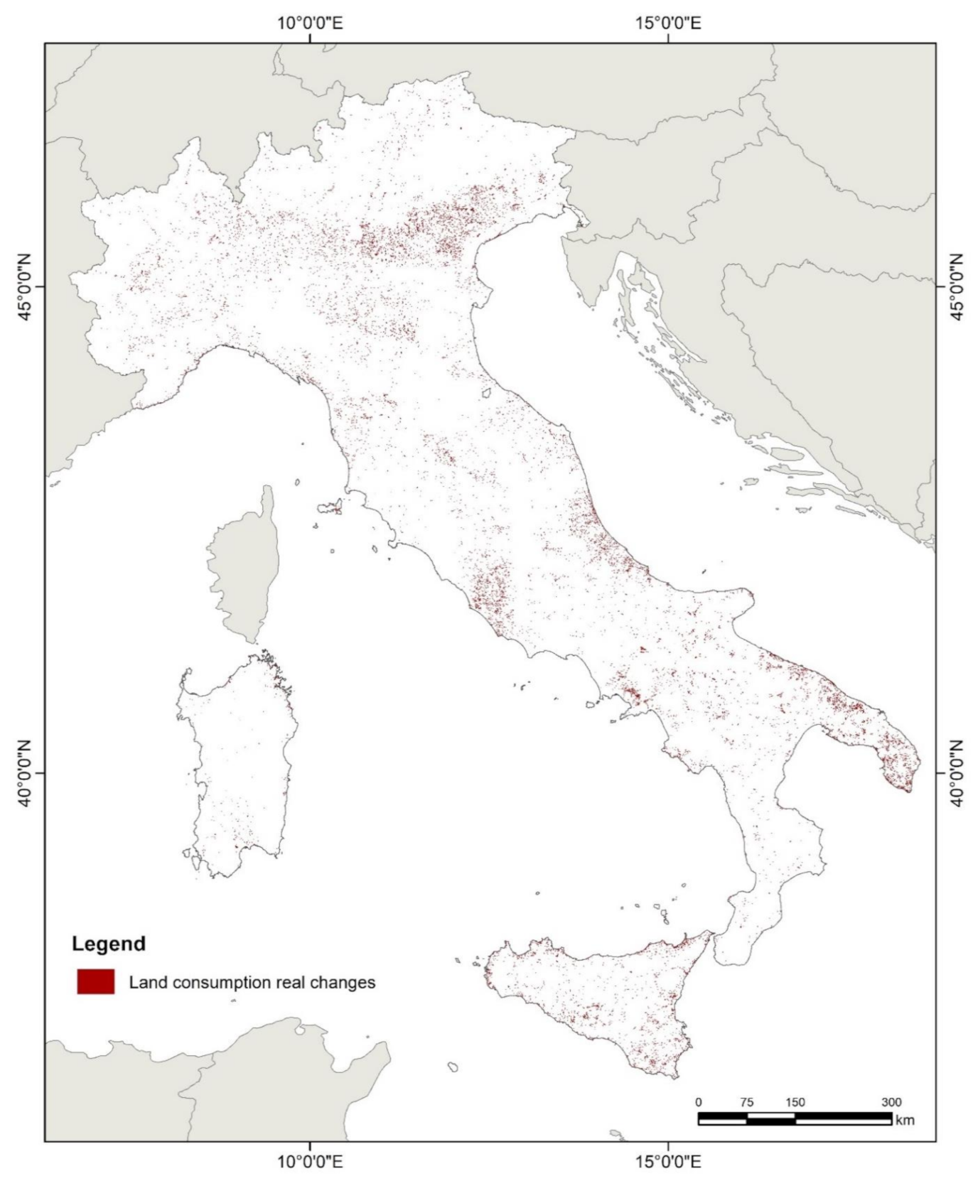
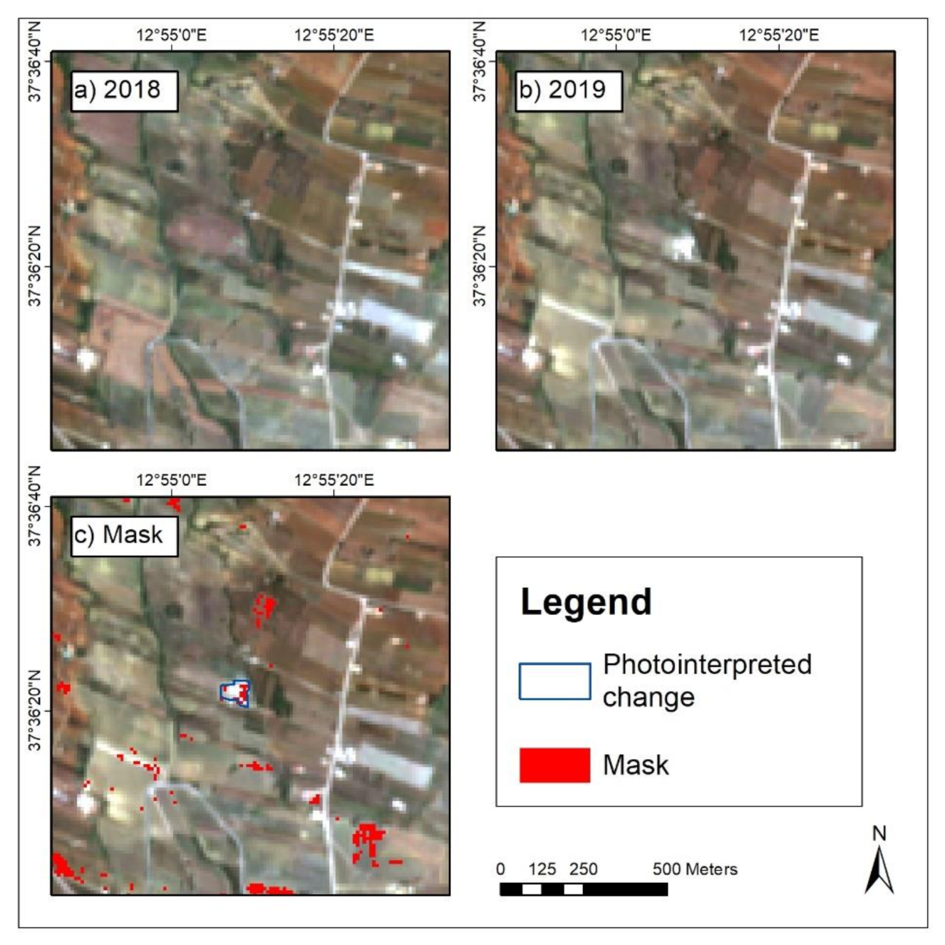
Comparison with the Real Changes Photointerpreted by ISPRA-SNPA

The three approaches results were compared to the land consumption map produced by ISPRA-SNPA for 2019. About 33,000 real changes were classified by ISPRA-SNPA by photointerpretation (Figure 9), covering about 57 km² of land consumed between 2018 and 2019 [57]. It should be noted that the photointerpretation was performed for the whole Italian territory, in order to classify all the real changes and assess errors, for each approach, due to the variability of geographical conditions.

The correspondence between real and potential changes was assessed both quantitatively and qualitatively. The assessment was also carried out at the pixel level, since the purpose of the methodology is to highlight the presence of potential change to the photointerpreter, which is in charge of outlining geometries (Figure 10).

The accuracies of three detection approaches when compared to interpreted changes are shown in

Table 2. Count of real changes identified by at least one pixel.

Approach	Undetected Changes	Detected Changes	Total	Percentage Of Detection
First	16245	16702	32947	50.7
Second	22742	10205	32947	31.0
Third	13257	19690	32947	59.8

. The highest overall accuracy was achieved in the third approach (59.8% of real changes detected), followed the first (50.7%), while the worst performance was obtained by the second (31%).

Filtering changes by their extension, considering only those above a threshold of 100 m² (i.e., one pixel), the first approach detection improved, detecting 58.9% of changes (

Table 3. Count of real changes with surface > 100 m² identified by at least one pixel.

Approach	Not Detected Changes	Detected Changes	Total	Percentage Of Detection
First	10163	14572	24735	58.9
Second	15426	9309	24735	37.6
Third	7332	17403	24735	70.4

). In the same way, the second approach resulted in 37.6% of changes detected. The highest percentage of detection was provided by the third approach (i.e., 70.4%). Therefore, as can be seen from the comparison between Table 2 and Table 3, the exclusion of single isolated pixels can lead to an improvement, justified by mixed pixel abundance, which is common, especially in coarse spatial resolution data. Single pixel omission, however, does not affect the detection of large areas that are usually highlighted by more than one pixel.

To better understand the relation between detected changes and change area, changes were grouped in classes based on the area (i.e., ≤100 m², between 100 and 500 m², between 500 and 1000 m², between 1000 and 1500 m², between 1500 and 2000 m², >2000 m²).

Table 4. Count of real changes identified in the third approach, by at least one pixel, grouped by class of area.

Class of Area	Not Detected Changes	Detected Changes	Percentage of Detection
≤100 m2	11983	11304	48.5
between 100 m2 and 500 m2	1126	6236	84.7
between 500 m2 and 1000 m2	113	1205	91.4
between 1000 m2 and 1500 m2	22	420	95.0
between 1500 m2 and 2000 m2	3	188	98.4
>2000 m2	10	337	97.1

illustrates the changes identified by the third approach. The number of changes detected by the masks exceeds 90% for changes larger than 500 m², reaching over 98% for the largest changes. The resumed results are also good for small changes (i.e., between 1 and 5 pixels), which are detected at almost 85%.

The omissions are mainly related to the smallest changes, which are less than one pixel in size. This is partly due to the reflectance of the mixed pixels. The larger omissions mainly concern photovoltaic fields, in which the NDVI does not reach the set thresholds. The main causes can be intuitively identified in mixed cover (bare soil between panels) and light-absorbing material behavior. Their detection is a further research direction proposal, as they are an important source of land consumption, especially in areas with significant irradiation values.

The third approach generated the largest number of changes and the largest surface to be investigated, due to the greater presence of false positives. In this sense, the use of the masks produced by the third approach requires the inspection of a 56% larger surface than that detected with the first approach (7300 against 3200 km²).

From the comparison between the interpreted changes (Figure 9) and the masks obtained with the third approach (Figure 8), it can be seen that the false positives are concentrated in Southern Italy.

In this regard, the introduction of the shift period made it possible to increase the percentage of changes detected in the northern regions, but has introduced numerous false changes, especially in the south of Italy. In fact, the use of two ranges of NDVI ("main range" and "additional range") allows us to distinguish the less probable changes during the photointerpretation process.

As illustrated in Figure 11, the NDVI method caused a false positive in agricultural fields that were vegetated in the first year and permanently plowed in the second year, resulting visually in exposing bare soil. Analogue issues were found with the method for detecting land consumption related to buildings and infrastructures using SAR data, due to the movement of large vehicles, such as trucks or buses, in parking lots.

However, the third approach is preferable, as it identifies most of the large changes, keeping the area to be inspected at 2.4% of the total national surface.

4. Discussion

The methodology was developed as part of the land consumption monitoring conducted by ISPRA for the whole Italian territory; therefore, the project requirements influenced this methodology.

The update must ensure very high accuracy values, since the current National Land Consumption Map has an overall accuracy of 99.7% [45]; therefore, it was conducted by means of both manual inspection of the entire national territory and photointerpretation of the changes.

The extent of the study area and in particular the required level of accuracy were a main constraint in the development of a change detection methodology based on photointerpretation.

Many methodologies based on supervised classification, as machine learning methods, allow excellent accuracy to be achieved, but they are still lower than the required values. Furthermore, the application of these methodologies on a large scale requires a huge number of training areas.

The proposed methodology is based on photointerpretation, identifying areas with potential changes and thus reducing the extent of the area that must be inspected by the photointerpreter. This method is, therefore, time-effective, as well as cost-effective, by significantly reducing costs for the purchase of VHR images.

In this sense, a set of rules based on conservative thresholds was defined, in order to favor limit omissions.

The additional project requirement of the reference period conditioned the definition of the thresholds. The updating of the data institutionally must be referred to a flexible time period between March and July (e.g., in order to detect changes that occurred between the nominal year and the previous one). It is worth highlighting that this flexible period allows the unavailability of very high-resolution images (with a precise acquisition date) during the photointerpretation of changes performed by ISPRA-SNPA to be overcome.

This period centered in May influenced several choices of the present methodology due to the impact of seasonality on the vegetation and, therefore, on the spectral characteristics of land before and after land consumption.

The first approach defines a series of basic conditions for the detection of land consumption, allowing for the identification of 58.9% of real changes larger than a pixel.

The second approach adds to the conditions of the first approach a raster condition based on Sentinel-1 data that tries to identify arable land. This was in order to exclude the arable land from change detection and further reduce the photointerpretation area to about 200 km². Nevertheless, this condition also excluded several actual changes (about 69% of real changes were omitted, equal to a decrease of 3000 km² of possible change area compared to the first approach) and did not respect the objective of avoiding omission errors.

The third approach applied the same methodology of the first approach with the addition of a shifted period starting from June, in order to also detect the changes that occurred after the start of year 2. This additional period increased the area of possible changes to about 7300 km², but provided the highest detection of land consumption (59.8% of the changes in the size of a pixel, 70.4% of those larger than one pixel and over 84% of those larger than 500 m²). The omission errors are mainly related to single pixel changes, which are difficult to detect due to the spectrally mixed pixel. Larger omissions are mainly related to land consumption over areas with scarce vegetation and very low NDVI in year 1, and, therefore, with a very low NDVI difference with year 2.

The third approach provides more flexibility in the monitoring of land consumption, also identifying changes between March and June and providing a code distinction of the most probable changes.

The developed methodology is based on the assumptions about the impact of land consumption on NDVI and backscatter values. The use of this methodology could be adapted to other European countries with a climate similar to Italy, adapting the thresholds and temporal ranges to local characteristics and vegetation phenology. In other countries where the climate is particularly arid, the above assumptions would be not valid, and therefore, the methodology would not be applicable, although this requires further studies.

The methodology is not designed to accurately detect the shape of changes but to support photointerpretation in their identification. This approach derives from the requirements imposed by ISPRA’s land consumption monitoring activity, in terms of accuracy, updating the frequency and extension of the study area.

The main products that provide information related to land consumption have characteristics and requirements different from the ISPRA’s product, which influence the adopted methodology for both the creation of the data itself and for the identification and changes.

Copernicus products offer a mapping of the land cover, with specific classes for the classification of land consumption, but they are updated with a much lower frequency than the ISPRA’s data and offer lower levels of accuracy. In detail, CORINE Land Cover [58] and Urban Atlas [59] are updated every six years through photointerpretation, while the HRLs are updated every three years [60] through the use of complex calculation tools and different types of data, many of which are not free and with resolutions higher than Sentinel (such as RapidEye data).

Several classification products have been developed to map urban land on a global scale, such as the Global Human Settlement Layer (GHSL) [61], the Global Urban Footprint (GUF) [62] or the Global human-made Impervious Surface (GMIS) [63]. While these and other datasets provide essential information about urbanization, they do not allow the monitoring of the phenomena, since they typically characterize it in specific points in time.

The developed methodology, while not allowing the direct mapping of land consumption, guarantees a 97.6% reduction in the area to be photointerpreted. The simplicity of calculation does not require the definition of training areas, compared to more refined methods, such as machine learning supervised methods.

5. Conclusions

This study developed a methodology to automatically detect land consumption, in order to ease and fasten the photointerpretation of actual changes in Italy that is performed by ISPRA-SNPA. The methodology uses Sentinel-1 and Sentinel-2 images, provided freely by Copernicus, acquired in two reference years to detect the land consumption that occurred in 1 year. The methodology was applied during the period from March to July, which was selected due to the ISPRA-SNPA institutional requirements.

The automatic workflow using decision trees and fixed threshold values allowed us to detect the changes that occurred between 2018 and 2019 in Italy, with a spatial resolution of 10 m. It is worth highlighting that the priority was to avoid omission errors, allowing commission errors (false changes) that will be photointerpreted and excluded from actual changes. The apparently large surface of possible changes (i.e., over 7000 km²) is about 2.3% of the Italian surface (e.g., about 302,000 km²), therefore reducing the photointerpretation effort to a very limited extent.

This methodology can substantially reduce the photointerpretation effort (focusing on changes highlighted by the automatic classification), and can allow for the use of Sentinel-2 RGB composites avoiding the cost of commercial images. Nevertheless, the use of very high-resolution images can improve the detection of small changes, especially considering that pixel size changes are often omitted by the automatic classification.

In the future, the integration of object segmentation of very high-resolution images could provide fully automatic mapping of changes, considering that this methodology would require mainly the red and infrared bands for NDVI calculation. Moreover, further research is required to overcome the omission errors of single pixel changes, especially for assessing how NDVI threshold values could improve the results, especially for mixed pixels. Finally, the purpose of reducing the extent of false positive changes will require more research in developing a methodology for masking areas such as the arable land affected by changes that are not related to land consumption.

References

1. European Commission. Thematic Strategy for Soil Protection, COM(2006)231; European Commission: Bruxelles, Belgium, 2006. [Google Scholar]
2. European Commission. Roadmap, New Soil Strategy—Healthy Soil for a Healthy Life; European Commission: Bruxelles, Belgium, 2020. [Google Scholar]
3. European Commission. The European Green Deal, COM(2019) 640 Final; European Commission: Bruxelles, Belgium, 2019. [Google Scholar]
4. European Commission. EU Biodiversity Strategy for 2030—Bringing Nature Back into our Lives, COM(2020) 380 Final; European Commission: Bruxelles, Belgium, 2020. [Google Scholar]
5. European Commission. A Farm to Fork Strategy for a Fair, Healthy and Environmentally-Friendly Food System, COM(2020) 381 Final; European Commission: Bruxelles, Belgium, 2020. [Google Scholar]
6. Scholes, R.J.; Montanarella, L.; Brainich, E.; Barger, N.; Ten Brink, B.; Cantele, M.; Erasmus, B.; Fisher, J.; Gardner, T.; Holland, T.G. IPBES (2018): Summary for Policymakers of the Assessment Report on Land Degradation and Restoration of the Intergovernmental Science-Policy Platform on Biodiversity and Ecosystem Services; The Intergovernmental Platform on Biodiversity and Ecosystem: Bonn, Germany, 2018. [Google Scholar]
7. Gardi, C.; Panagos, P.; Van Liedekerke, M.; Bosco, C.; De Brogniez, D. Land take and food security: Assessment of land take on the agricultural production in Europe. J. Environ. Plan. Manag. 2015, 58, 898–912. [Google Scholar] [CrossRef]
8. Imhoff, M.; Lahouari, B.; Taylor, R.; Colby, L.; Robert, H.; William, L. Global patterns in human consumption of net primary production. Nature 2004, 429, 867–870. [Google Scholar] [CrossRef] [PubMed] [Green Version]
9. Bennett, A.F.; Saunders, D.A. Habitat fragmentation and landscape change. Conserv. Biol. All 2010, 93, 1544–1550. [Google Scholar]
10. Ruby, E. How Urbanization Affects the Water Cycle. California Water and Land Use Partnership. Available online: http://www.coastal.ca.gov/nps/watercyclefacts.pdf (accessed on 7 December 2020).
11. EEA. The European Environment—State and Outlook 2020 Knowledge for Transition to a Sustainable Europe; European Environment Agency: Copenhagen, Denmark, 2019. [Google Scholar]
12. Arnold, S.; Kosztra, B.; Banko, G.; Milenov, P.; Smith, G.; Hazeu, G. Explanatory Documentation of the EAGLE Concept. European Environment Agency: Copenhagen, Denmark. 2020. Available online: https://land.copernicus.eu/eagle/files/explanatory-documentation/eagle-concept-explanatory-documentation-version-3-1-4-12-2020/view (accessed on 4 March 2021).
13. Strollo, A.; Smiraglia, D.; Bruno, R.; Assennato, F.; Congedo, L.; De Fioravante, P.; Giuliani, C.; Marinosci, I.; Riitano, N.; Munafò, M. Land consumption in Italy. J. Maps 2020, 16, 113–123. [Google Scholar] [CrossRef]
14. European Parliament, Council of the European Union. European Union Decision No 1386/2013/EU of the European Parliament and of the Council of 20 November 2013 on a General Union Environment Action Programme to 2020 “Living well, within the limits of our planet. Off. J. Eur. Union 2013, 353, 171–200. [Google Scholar]
15. European Parliament, Council of the European Union. European Commision Parliament Commission Delegated Regulation (EU) No 1159/2013 of 12 July 2013. Off. J. Eur. Union 2013, 309, 1–6. [Google Scholar]
16. Lefebvre, A.; Sannier, C.; Corpetti, T. Monitoring urban areas with Sentinel-2A data: Application to the update of the Copernicus high resolution layer imperviousness degree. Remote Sens. 2016, 8, 606. [Google Scholar] [CrossRef] [Green Version]
17. Forkuor, G.; Dimobe, K.; Serme, I.; Tondoh, J.E. Landsat-8 vs. Sentinel-2: Examining the added value of sentinel-2’s red-edge bands to land-use and land-cover mapping in Burkina Faso. GIScience Remote Sens. 2018, 55, 331–354. [Google Scholar] [CrossRef]
18. Singh, A. Review article digital change detection techniques using remotely-sensed data. Int. J. Remote Sens. 1989, 10, 989–1003. [Google Scholar] [CrossRef] [Green Version]
19. Coppin, P.; Jonckheere, I.; Nackaerts, K.; Muys, B.; Lambin, E. Review ArticleDigital change detection methods in ecosystem monitoring: A review. Int. J. Remote Sens. 2004, 25, 1565–1596. [Google Scholar] [CrossRef]
20. Reba, M.; Seto, K.C. A systematic review and assessment of algorithms to detect, characterize, and monitor urban land change. Remote Sens. Environ. 2020, 242, 111739. [Google Scholar] [CrossRef]
21. Zhu, Z. Change detection using landsat time series: A review of frequencies, preprocessing, algorithms, and applications. ISPRS J. Photogramm. Remote Sens. 2017, 130, 370–384. [Google Scholar] [CrossRef]
22. Ban, Y.; Yousif, O. Change detection techniques: A review. In Multitemporal Remote Sensing; Springer: Berlin/Heidelberg, Germany, 2016; pp. 19–43. [Google Scholar]
23. Radke, R.J.; Andra, S.; Al-Kofahi, O.; Roysam, B. Image change detection algorithms: A systematic survey. IEEE Trans. Image Process. 2005, 14, 294–307. [Google Scholar] [CrossRef]
24. Hussain, M.; Chen, D.; Cheng, A.; Wei, H.; Stanley, D. Change detection from remotely sensed images: From pixel-based to object-based approaches. ISPRS J. Photogramm. Remote Sens. 2013, 80, 91–106. [Google Scholar] [CrossRef]
25. Lu, D.; Li, G.; Moran, E. Current situation and needs of change detection techniques. Int. J. Image Data Fusion 2014, 5, 13–38. [Google Scholar] [CrossRef]
26. Lu, D.; Mausel, P.; Brondizio, E.; Moran, E. Change detection techniques. Int. J. Remote Sens. 2004, 25, 2365–2401. [Google Scholar] [CrossRef]
27. Tewkesbury, A.P.; Comber, A.J.; Tate, N.J.; Lamb, A.; Fisher, P.F. A critical synthesis of remotely sensed optical image change detection techniques. Remote Sens. Environ. 2015, 160, 1–14. [Google Scholar] [CrossRef] [Green Version]
28. Karantzalos, K. Recent advances on 2D and 3D change detection in urban environments from remote sensing data. In Computational Approaches for Urban Environments; Springer: Berlin/Heidelberg, Germany, 2015; pp. 237–272. [Google Scholar]
29. Hansen, M.C.; Loveland, T.R. A review of large area monitoring of land cover change using Landsat data. Remote Sens. Environ. 2012, 122, 66–74. [Google Scholar] [CrossRef]
30. Gamba, P.; Dell’Acqua, F. Change detection in urban areas: Spatial and temporal scales. In Multitemporal Remote Sensing; Springer: Berlin/Heidelberg, Germany, 2016; pp. 45–61. [Google Scholar]
31. Moser, G.; Serpico, S.B. Generalized minimum-error thresholding for unsupervised change detection from SAR amplitude imagery. IEEE Trans. Geosci. Remote Sens. 2006, 44, 2972–2982. [Google Scholar] [CrossRef]
32. He, C.; Wei, A.; Shi, P.; Zhang, Q.; Zhao, Y. Detecting land-use/land-cover change in rural–urban fringe areas using extended change-vector analysis. Int. J. Appl. Earth Obs. Geoinf. 2011, 13, 572–585. [Google Scholar] [CrossRef]
33. Bovolo, F.; Bruzzone, L. A split-based approach to unsupervised change detection in large-size multitemporal images: Application to tsunami-damage assessment. IEEE Trans. Geosci. Remote Sens. 2007, 45, 1658–1670. [Google Scholar] [CrossRef]
34. Thonfeld, F.; Feilhauer, H.; Braun, M.; Menz, G. Robust Change Vector Analysis (RCVA) for multi-sensor very high resolution optical satellite data. Int. J. Appl. Earth Obs. Geoinf. 2016, 50, 131–140. [Google Scholar] [CrossRef]
35. Deng, J.S.; Wang, K.; Deng, Y.H.; Qi, G.J. PCA-based land-use change detection and analysis using multitemporal and multisensor satellite data. Int. J. Remote Sens. 2008, 29, 4823–4838. [Google Scholar] [CrossRef]
36. Volpi, M.; Tuia, D.; Bovolo, F.; Kanevski, M.; Bruzzone, L. Supervised change detection in VHR images using contextual information and support vector machines. Int. J. Appl. Earth Obs. Geoinf. 2013, 20, 77–85. [Google Scholar] [CrossRef]
37. Nemmour, H.; Chibani, Y. Multiple support vector machines for land cover change detection: An application for mapping urban extensions. ISPRS J. Photogramm. Remote Sens. 2006, 61, 125–133. [Google Scholar] [CrossRef]
38. Ban, Y.; Webber, L.; Gamba, P.; Paganini, M. EO4Urban: Sentinel-1A SAR and Sentinel-2A MSI data for global urban services. In Proceedings of the 2017 Joint Urban Remote Sensing Event (JURSE), Dubai, United Arab Emirates, 6–8 March 2017; pp. 1–4. [Google Scholar]
39. Pesaresi, M.; Corbane, C.; Julea, A.; Florczyk, A.J.; Syrris, V.; Soille, P. Assessment of the added-value of sentinel-2 for detecting built-up areas. Remote Sens. 2016, 8, 299. [Google Scholar] [CrossRef] [Green Version]
40. Haas, J.; Ban, Y. Sentinel-1A SAR and sentinel-2A MSI data fusion for urban ecosystem service mapping. Remote Sens. Appl. Soc. Environ. 2017, 8, 41–53. [Google Scholar] [CrossRef]
41. Goldblatt, R.; Deininger, K.; Hanson, G. Utilizing publicly available satellite data for urban research: Mapping built-up land cover and land use in Ho Chi Minh City, Vietnam. Dev. Eng. 2018, 3, 83–99. [Google Scholar] [CrossRef]
42. Celik, N. Change detection of urban areas in Ankara through Google Earth engine. In Proceedings of the 2018 41st International Conference on Telecommunications and Signal Processing (TSP), Athens, Greece, 4–6 July 2018; pp. 1–5. [Google Scholar]
43. Sun, Z.; Xu, R.; Du, W.; Wang, L.; Lu, D. High-resolution urban land mapping in China from sentinel 1A/2 imagery based on Google Earth Engine. Remote Sens. 2019, 11, 752. [Google Scholar] [CrossRef] [Green Version]
44. Iannelli, G.C.; Gamba, P. Jointly exploiting Sentinel-1 and Sentinel-2 for urban mapping. In Proceedings of the IGARSS 2018–2018 IEEE International Geoscience and Remote Sensing Symposium, Valencia, Spain, 22–27 July 2018; pp. 8209–8212. [Google Scholar]
45. Munafò, M. Consumo di Suolo, Dinamiche Territoriali e Servizi Ecosistemici. Available online: https://www.snpambiente.it/wp-content/uploads/2019/09/Rapporto_consumo_di_suolo_20190917-1.pdf (accessed on 4 March 2021).
46. Joshi, N.; Baumann, M.; Ehammer, A.; Fensholt, R.; Grogan, K.; Hostert, P.; Jepsen, M.R.; Kuemmerle, T.; Meyfroidt, P.; Mitchard, E.T.A.; et al. A review of the application of optical and radar remote sensing data fusion to land use mapping and monitoring. Remote Sens. 2016, 8, 70. [Google Scholar] [CrossRef] [Green Version]
47. Cao, Y.; Su, C.; Yang, G. Detecting the number of buildings in a single high-resolution SAR image. Eur. J. Remote Sens. 2014, 47, 513–535. [Google Scholar] [CrossRef] [Green Version]
48. Nezry, E. Adaptive speckle filtering in radar imagery. In Land Applications of Radar Remote Sensing; IntechOpen: London, UK, 2014; pp. 1–55. [Google Scholar]
49. Holtgrave, A.K.; Röder, N.; Ackermann, A.; Erasmi, S.; Kleinschmit, B. Comparing Sentinel-1 and -2 data and indices for agricultural land use monitoring. Remote Sens. 2020, 12, 2919. [Google Scholar] [CrossRef]
50. Hoskera, A.K.; Nico, G.; Irshad Ahmed, M.; Whitbread, A. Accuracies of soil moisture estimations using a semi-empirical model over bare soil agricultural croplands from sentinel-1 SAR data. Remote Sens. 2020, 12, 1664. [Google Scholar] [CrossRef]
51. Coluzzi, R.; Imbrenda, V.; Lanfredi, M.; Simoniello, T. A first assessment of the Sentinel 2 Level 1-C cloud mask product to support informed surface analyses. Remote Sens. Environ. 2018, 217, 426–443. [Google Scholar] [CrossRef]
52. Spadoni, G.L.; Cavalli, A.; Congedo, L.; Munafò, M. Analysis of Normalized Difference Vegetation Index (NDVI) multi-temporal series for the production of forest cartography. Remote Sens. Appl. Soc. Environ. 2020, 20, 100419. [Google Scholar]
53. Ballère, M.; Bouvet, A.; Mermoz, S.; Le Toan, T.; Koleck, T.; Bedeau, C.; André, M.; Forestier, E.; Frison, P.-L.; Lardeux, C. SAR data for tropical forest disturbance alerts in French Guiana: Benefit over optical imagery. Remote Sens. Environ. 2021, 252, 112159. [Google Scholar] [CrossRef]
54. Formaggio, A.R.; Epiphanio, J.C.N.; Simões, M.D.S. Radarsat backscattering from an agricultural scene. Pesq. Agropec. Bras. 2001, 36, 823–830. [Google Scholar] [CrossRef] [Green Version]
55. Koppel, K.; Zalite, K.; Voormansik, K.; Jagdhuber, T. Sensitivity of Sentinel-1 backscatter to characteristics of buildings. Int. J. Remote Sens. 2017, 38, 6298–6318. [Google Scholar] [CrossRef]
56. Jarvis, A.; Guevara, E.; Reuter, H.I.; Nelson, A.D. Hole-filled SRTM for the globe: Version 4: Data grid; GIAR Consortium for Spatial Information: Washington, DC, USA, 2008. Available online: http://srtm.csi.cgiar.org/ (accessed on 15 February 2021).
57. Munafò, M. Consumo di Suolo, Dinamiche Territoriali e Servizi Ecosistemici. Edizione 2020; SNPA: Rome, Italy, 2020; p. 291. ISBN 9788844810139. [Google Scholar]
58. Büttner, G.; Kostztra, B.; Soukup, T.; Sousa, A.; Langanke, T. CLC2018 Technical Guidelines; European Environment Agency: Copenhagen, Denmark, 2017; pp. 1–60. [Google Scholar]
59. European Commission for European Mapping Guide Urban Atlas, 2016, 1–39. Available online: https://land.copernicus.eu/user-corner/technical-library/urban-atlas-mapping-guide (accessed on 28 February 2021).
60. Lefebvre, A.; Beaugendre, N.; Pennec, A.; Sannier, C.; Corpetti, T. Using data fusion to update built-up areas of the 2012 European High-Resolution Layer Imperviousness. In Proceedings of the 33rd EARSeL Symposium Conference, Matera, Italy, 3–6 June 2013; Volume 36, p. 321328. [Google Scholar]
61. Pesaresi, M.; Huadong, G.; Blaes, X.; Ehrlich, D.; Ferri, S.; Gueguen, L.; Halkia, M.; Kauffmann, M.; Kemper, T.; Lu, L.; et al. A global human settlement layer from optical HR/VHR RS data: Concept and first results. IEEE J. Sel. Top. Appl. Earth Obs. Remote Sens. 2013, 6, 2102–2131. [Google Scholar] [CrossRef]
62. Esch, T.; Heldens, W.; Hirner, A.; Keil, M.; Marconcini, M.; Roth, A.; Zeidler, J.; Dech, S.; Strano, E. Breaking new ground in mapping human settlements from space—The Global Urban Footprint. ISPRS J. Photogramm. Remote Sens. 2017, 134, 30–42. [Google Scholar] [CrossRef] [Green Version]
63. Brown de Colstoun, E.C.; Huang, C.; Wang, P.; Tilton, J.C.; Tan, B.; Phillips, J.; Niemczura, S.; Ling, P.-Y.; Wolfe, R.E. Global Man-Made Impervious Surface (GMIS) Dataset From Landsat 2017; NASA Socioeconomic Data and Applications Center: Palisades, NY, USA, 2017. [Google Scholar]
64. Arnold, S.; Kosztra, B.; Banko, G.; Milenov, P.; Smith, G.; Hazeu, G. Explanatory Content Documentation of the EAGLE Concept [2021, version 3.1]. Available online: https://land.copernicus.eu/eagle/content-documentation-of-the-eagle-concept/manual/eagle-explanatory-documentation-v3-1-version-2021 (accessed on 4 March 2021).
65. European Parliament and of the Council of the European Union. Directive 2007/2/EC of the European Parliament and of the Council of 14 March 2007 establishing an Infrastructure for Spatial Information in the European Community (INSPIRE); European Parliament and of the Council of the European Union: Bruxelles, Belgium, 2007; pp. 1–14. [Google Scholar]
Figure 1. Overview of the classification methodology.
Remotesensing 13 01586 g001
Figure 2. Workflow of the methodology of land consumption related to vegetation removal with arable land filter.
Remotesensing 13 01586 g002
Figure 3. Scheme of change that occurred between start date 1 and start date 2 detected by the methodology; the upper chart represents the NDVI values of a pixel at different acquisition times; the lower chart represents the maximum NDVI value resulting from the acquisition periods of the 2 years.
Remotesensing 13 01586 g003
Figure 4. Scheme of change occurred after start date 2 that can be identified with the shift period.
Remotesensing 13 01586 g004
Figure 5. Workflow of the methodology of land consumption related to vegetation removal with the shift period.
Remotesensing 13 01586 g005
Figure 6. Workflow of the methodology of land consumption related to buildings and infrastructures.
Remotesensing 13 01586 g006
Figure 7. Land consumption example related to buildings and infrastructures. Images (a) and (b) show the Sentinel-2 image for 2018 and 2019; image (c) reports the potential change identified by the mask; images (dh) indicate the areas where the considered conditions are verified (green) and not verified (grey). The information related to the slope is not shown, as the whole area illustrated has a slope of <20%.
Remotesensing 13 01586 g007
Figure 8. Raster of the possible land consumption produced by the third approach.
Remotesensing 13 01586 g008
Figure 9. Land consumption changes (2018–2019) monitored by ISPRA-SNPA.
Remotesensing 13 01586 g009
Figure 10. Example of change photointerpreted by ISPRA-SNPA and the change detected with the developed methodology. (a) Copernicus Sentinel-2 image (2018) before the land consumption highlighted with blue contour; (b) Copernicus Sentinel-2 image (2019) after the land consumption. (c) The area of potential changes identified with the third approach (yellow) is compared with the photointerpreted polygon (blue).
Remotesensing 13 01586 g010
Figure 11. Example of commission errors in the masks obtained by applying the third approach. (a) Copernicus Sentinel-2 image (2018) before the land consumption; (b) Copernicus Sentinel-2 image (2019) after the land consumption. (c) The area inside the blue polygon represents a true change correctly detected, while the other red areas are commission errors of the mask.
Remotesensing 13 01586 g011