Article

Evaluation of Total Ozone Column from Multiple Satellite Measurements in the Antarctic Using the Brewer Spectrophotometer

1
Department of Atmospheric Sciences, Yonsei University, Seoul 03722, Korea
2
Korea Polar Research Institute, Incheon 21990, Korea
3
Harvard-Smithsonian Center for Astrophysics, Cambridge, MA 02140, USA
*
Author to whom correspondence should be addressed.
Submission received: 22 February 2021 / Revised: 1 April 2021 / Accepted: 15 April 2021 / Published: 20 April 2021

Abstract

:
The ground-based ozone observation instrument, Brewer spectrophotometer (Brewer), was used to evaluate the quality of the total ozone column (TOC) produced by multiple polar-orbit satellite measurements at three stations in Antarctica (King Sejong, Jang Bogo, and Zhongshan stations). While all satellite TOCs showed high correlations with Brewer TOCs (R = ~0.8 to 0.9), there are some TOC differences among satellite data in austral spring, which is mainly attributed to the bias of Atmospheric Infrared Sounder (AIRS) TOC. The quality of satellite TOCs is consistent between Level 2 and 3 data, implying that “which satellite TOC is used” can induce larger uncertainty than “which spatial resolution is used” for the investigation of the Antarctic TOC pattern. Additionally, the quality of satellite TOC is regionally different (e.g., OMI TOC is a little higher at the King Sejong station, but lower at the Zhongshan station than the Brewer TOC). Thus, it seems necessary to consider the difference of multiple satellite data for better assessing the spatiotemporal pattern of Antarctic TOC.

Graphical Abstract

1. Introduction

Since the early 1980s, when ozone depletion in the Antarctic stratosphere was first detected [1], the Antarctic stratospheric ozone hole has been continuously monitored and has emerged as a global environmental problem. Chlorofluorocarbons released by human activities act as a catalyst for ozone destruction, forming stratospheric ozone holes [2], inducing the increase in harmful solar radiation at the surface. The formation of the ozone hole also relates to the pattern of atmospheric dynamics and regional meteorology [3]. Particularly, several studies revealed that the stratospheric ozone variation is a major factor influencing the Southern Annular Mode (SAM), a type of large-scale atmospheric circulation in the southern hemisphere [4,5]. Changes in the SAM cause the variation in the mid-latitude jet flow, which not only influences the tropospheric–stratospheric mass exchange [6,7] but also the Antarctic sea ice distribution [8] and even temperature and precipitation in Australia [9,10]. Thus, it is very important to continuously monitor the stratospheric ozone pattern as its depletion affects both the Antarctic stratosphere and the lower atmosphere in Antarctica, Australia, and the southern hemisphere [11].
The Brewer spectrophotometer (hereafter, Brewer) is a ground-based remote sensing instrument widely used for stratospheric ozone monitoring, based on the measurement of total ozone column (TOC) from direct sun and zenith sky techniques. Previous studies reported that Brewer is a high-performance stratospheric ozone observation device with an accuracy of 1% error in direct sun mode and less than 3%–5% error in zenith sky scattered mode [12]. The Brewer has also provided reliable data at various ozone monitoring stations in Antarctica [13], but the ground-based measurement still has spatial limitations. The utilization of satellite data can be a solution to overcome this limitation, which allows the coverage of large areas. In particular, the usage of satellite TOC values enables us to examine the relationship to the regional meteorology in the broad area [14].
Fortunately, it is possible to sufficiently track changes in the amount of stratospheric ozone using satellites; several satellite observations have been carried out to date. Satellite observation data must be verified through comparison with ground-based instrument data to ensure quality and reliability [15]. A number of ground-based instruments have been used for the validation of satellite TOC observations, e.g., Dobson spectrophotometer [16,17,18]; Brewer spectrophotometer [19,20,21]; SAOZ [22,23,24]; Pandora photometer [25,26,27]; and ozonesonde [28,29,30]. Inter-comparison between the data collected by ground-based instruments and satellite data to analyze the changes of ozone amount has also been performed [31,32,33,34]. As shown above, the Brewer is commonly used for inter-comparison studies [35,36]. However, the verification of satellite data has not been performed much in the polar region because of the operational difficulties in ground-based observation in the harsh cold condition. While a few related studies performed recently [37,38], further validations are much required. Thus, there is a need to secure new data for the comparative verification.
In this study, we verified the TOCs observed from multiple satellites using several Brewer TOCs. First, we used Brewer data at two Korean stations (King Sejong and Jang Bogo station), which have not been extensively considered in previous studies. Ozone monitoring record is especially rare in the Antarctic region nearby the Ross Sea where the Jang Bogo station is located. Hence, it is believed that ozone monitoring at the Jang Bogo station could provide valuable insights associated with the analysis of the Antarctic stratospheric ozone. Second, in order to cover the whole Antarctic region evenly, we also used the Brewer data at the Zhongshan station, which has been often used for the Antarctic TOC analysis [39,40,41,42]. Using these Brewer TOC data, we would evaluate the quality of TOC from the measurement of multiple satellite instruments: The Ozone Monitoring Instrument (OMI), TROPOspheric Monitoring Instrument (TROPOMI), Global Ozone Monitoring Experiment-2 (GOME-2), Ozone Mapping and Profiler Suite (OMPS), and Atmospheric Infrared Sounder (AIRS). We mainly examined the correlations of TOC values between the Brewer and satellite observations, then also assessed other statistic values. Through this research, we aimed to show the necessity of using various TOC measurements simultaneously for the better diagnosis of target situations.

2. Data

2.1. Ground-Based TOC Measurement Using the Brewer

The Brewer observes the direct sun (DS mode) and zenith sky scattered (ZS mode) sunlight following a set operating schedule. This radiative observation is applied to retrieve the quantity of some trace gases in the atmosphere, e.g., ozone [43,44]. The Brewer consists of a single diffraction grating, five light emission slits, and a focal plane, and the absorption wavelengths of the slits used are 306.3, 310.1, 313.5, 316.0, and 320.0 nm, which are optimized to observe O3 and SO2. Compared to the ZS mode observation, it is known that the DS mode observation yields more accurate values; numerically, the errors of DS and ZS observation are less than 1% and 3%, respectively [44,45].
In this study, we used the Brewer TOC at three Antarctic stations: King Sejong, Jang Bogo, and Zhongshan stations (Figure 1). The Korea Polar Research Institute installed Brewers at the King Sejong station in 1996 (MK IV model) and the Jang Bogo station in 2014 (MK III model). In the Zhongshan station, built in 1989 as the second Antarctic science base of China, the MK IV Brewer was installed in 1993 and operated until 2010. After the end of MK IV operation, the TOC has been monitored using the MK III Brewer, which was newly installed in 2009 [46]. All available Brewer TOC data here can be obtained from the World Ozone and Ultraviolet Radiation Data Center (WOUDC), one of six world data centers operated by the Global Atmosphere Watch of the World Meteorological Organization. All these data are summarized in Table 1.
The observation periods for TOC Brewer data at the King Sejong, Jang Bogo, and Zhongshan stations were from January 23, 1998, to February 29, 2020 (excluding 2015 and 2017 due to a mechanical failure), from August 05, 2016 to March 10, 2020, and from March 16, 2000 to November 30, 2019 (excluding 2008–2012 and 2015 due to mechanical failure), respectively. The two Korean Antarctic stations provide daily average TOC values for both DS and ZS mode observations, while the Zhongshan station provides either a TOC from the DS or ZS mode observation as the daily representative (i.e., DS and ZS mode TOC values are not separately provided. When the TOC from the DS mode was available, TOC from the ZS mode was not provided). Despite this difference, the correlation coefficients between satellite and Brewer data for this station were similar with those of previous studies [41] and were therefore considered acceptable.
For the quality maintenance of Brewer data, there have been several instances of instrument calibration and inspection. After the initial installation, Brewer at the King Sejong station performed three instrument calibrations in 2004, 2013, and 2017 following the official process of the International Ozone Services, Inc. (IOS). Brewer at the Jang Bogo station performed an instrument calibration in 2014 following the official process of the Kipp and Zonen. The record of Brewer calibration at the Zhongshan station was provided in [46], addressing that main calibration was performed in Canada during 2000, and inter-comparison between two different Brewer instruments (MK III and MK IV) at the same site from 2009 to 2010. Based on these records, we decided that observations of three Brewers used in this study were qualified and proper for the comparison with satellite TOCs.

2.2. Satellite TOC measurement

2.2.1. OMI/Aura

The OMI sensor onboard the Aura satellite is the next generation ozone observation sensor following the Total Ozone Mapping Spectrometer (TOMS) and was developed using the TOMS version 8 algorithm [47] to observe the TOC and the vertical ozone profile. The main components of observation are O3, NO3, SO2, OCIO, BrO and aerosols. As a solar synchronous orbital satellite and a polar orbital satellite, OMI passes the equator when observed with the sun’s reflection angle at 13:45, and observes the entire Earth in one day by gradually shifting longitude according to the Earth’s rotation. The OMI sensor uses two ultraviolet channels (UV1: 270–314 nm, UV2: 360–380 nm) and one visible light channel (350–500 nm). The average spectral resolutions for full width at half maximum in the ultraviolet channels are 0.42 nm and 0.45 nm, respectively, and that of the visible light channel is 0.63 nm [48]. The OMI Level 2 TOC product [49] used in this study has a cross-track field of view (FOV) angle of 114° and an observation width of 2600 km, which is sufficient to observe the entire earth in one day. In addition, the OMI sensor has a spatial resolution of 13 km × 24 km by the nadir scanning method and performs an observation in a zoom mode of 13 km × 12 km. We also used the OMI Level 3 product data [50] in this study, which have a spatial resolution of 1.0° × 1.0°. This was produced from Level 2G data (0.25° × 0.25°), obtained by collecting the daily Level 2 data and taking quality-weighted average using grid data adjacent to the observed location.
Compared to other observational spectroscopic sensors, the OMI sensor has higher accuracy in detecting the chemical composition of clouds and the troposphere with improved resolution. The quality flag value is provided with TOC values; The value of 0 corresponding to the “good sample”, which was used to perform the comparison [50]. Previous studies have reported that the error of the OMI TOC is ~2% or 6 Dobson units (DU) and is ~25% of the observed value of tropospheric ozone [51]. In addition, as the solar zenith angle increases, the TOC in the upper troposphere may be overestimated due to several reasons: noise in the observation signal, temperature deviation between regions, decrease in sensitivity of the ozone signal, and the curvature effect of the Earth’s atmosphere. For these reasons, the expected values of the root mean square error (RMSE) for the TOC profile are estimated to be ~1.5%, 3%, and 5% for ≤70°, ≤82°, and ≤85°, respectively [52].

2.2.2. TROPOMI/S-5P

The TROPOMI onboard the Sentinel-5 Precursor (S-5P) satellite was launched on October 13, 2017. The satellite maintains an altitude of 824 km and passes through the equator at 13:30 local solar time. It travels 7 km/s and uses a two-dimensional observation device to have across-track and along-track observation resolutions of 3.5–15 km and 7 km, respectively with an observation width (swath) of 2600 km. It divides the wavelength of the input light into four sections using a grating spectrophotometer (UV–VIS–NIR–SWIR, UVNS) and specifies the wavelength range for each absorption band (UV and visible: 270–500 nm, near-infrared (NIR): 675–775 nm, short-wave infrared (SWIR): 2305–2385 nm) to perform the observation [53]. Compared to the absorption wavelength range of OMI sensors, the range of the TROPOMI is wider in the NIR and SWIR regions [54].
The spatial resolution of SWIR is 7 km × 7 km and that of others is 7 km × 3.5 km. Similar to the OMI data, the observed atmospheric chemicals from the TROPOMI measurement are O3, NO2, SO2, CO, CH4, aerosols and also clouds [53]. S-5P Level 2 data were provided at a resolution of 7 km × 3.5 km until December 27, 2019, and 5 km × 3.5 km thereafter. The TROPOMI algorithm used to calculate the total tropospheric ozone in this study is based on the one-step non-time critical or offline (OFFL) dataset (S5P_TO3_GODFIT) [55,56]. The value of quality flags was also applied for the TROPOMI Level 2 data. Following the product user’s guide [53], we only utilized the TOC having flag values > 50 among the flag values between 0 (no data) and 100 (full quality data). According to the results of previous studies on the observation accuracy and precision of TROPOMI for the global region, the error was 3% and 1% for the TOC, 10% and 5% for the ozone profile, and 25% and 10% for the total amount of tropospheric ozone, respectively [57].

2.2.3. OMPS/Suomi NPP

The OMPS sensor is onboard a polar orbit satellite, Suomi NPP (National Polar Orbiting Partnership) and performs one limb observation and two nadir observations. Among them, the nadir mapper system monitors the TOC while covering the entire sunlit orbit throughout the day; the nadir profiler and limb profiler observe the vertical ozone profiles for the outer regions of each sunlit orbit [58]. The OMPS has a cross-track FOV of 110° and a slit width of 0.27° along the orbit. According to cross-track observation, 35 pieces which were captured in one observation have a vertical width of 3.35° (50 km), and the resolution of along-track observation is 50 km. Concurrently, the TOC is observed by covering the observation width of 2800 km with nadir mapping for 7.6 s. Therefore, the resolutions of the OMPS Level 2 [59] swath and Level 3 [60] grid are 50 km × 50 km and 1° × 1°, respectively [58]. The total daily average ozone value was calculated using the TOMS version 7 algorithm [61]. The quality flags of the OMPS Level 2 output are provided in 16-bit format. Among them, the “good sample” value corresponding to the 0 value of the 0-bit was used. For the retrieval of the ozone amount, the wavelength regions with high ozone sensitivity (308.5, 310.5, 312.0, 312.5, 314.0, 315.0, 316.0, 317.0, 318.0, 320.0, 322.5, 325.0, 328.0, and 331.0 nm) and those with weaker sensitivity (321.0, 329.0, 332.0, 336.0 nm) were used simultaneously [58].

2.2.4. AIRS/Aqua

The AIRS sensor is onboard the Aqua satellite, a solar synchronous orbiting satellite that has been observing the polar region since March 4, 2002. The output of Level 2 data [62] used in this study has a pixel resolution of 50 km × 50 km and Level 3 [63] has a grid resolution of 1° × 1°. AIRS sensor also provides the TOC data as a daily average value. One big difference from previous satellite observations is the usage of longer wavelengths. The AIRS sensor has 2378 absorption channels in the infrared (IR) wavelength range of 3.75–15.4 μm and four absorption channels in the visible wavelength range of 0.4–1.0 μm. Additionally, the Advanced Microwave Sounding Unit–A (AMSU-A) device onboard the Aqua satellite has 15 microwave (MW) channels. The TOC value was calculated by combining the observed radiations in these IR/MW wavelength ranges based on day (ascending) and night (descending) monitoring. Level 2 output used in the study was prepared using only the values obtained during the day. The range of the quality flag values for each calculated TOC is 0–2 [64], and we only used the qualified TOC values (quality flag = 0).

2.2.5. GOME-2/MetOp

The GOME-2 sensor, as an optical spectrometer, is composed of four observational unit sections in the wavelength range of 240–790 nm. The optical spectrometers are equipped with scanning mirrors for omnidirectional observation in the nadir and across-track directions to cover the entire polar region [65].
The GOME-2 sensors have been on board a set of sun-synchronous and polar-orbital satellites passing through the equator at 09:30 UTC: EUMETSAT’s MetOp-A (launched in 2006), MetOp-B (launched in 2012) and MetOp-C (launched in 2018), respectively. Here, we used TOC from the measurements of GOME-2 onboard MetOp-A, retrieved from the GOME Data Processor (GDP) 4.8 algorithm. The GDP 4.8 algorithm is based on the typical optimized differential optical absorption spectroscopy (DOAS) method to convert the inclined observation value into a vertical value by applying an air mass factor (AMF) [66] for the retrieval of TOC and other trace gases (e.g., NO2, BrO, HCHO, SO2, etc.). For the TOC retrieval, the wavelength absorption range of the ozone absorption band (325–335 nm) was used for the ozone absorption band [67] with the 1.5%–2.0% of biases.
GOME-2 measurements are maintained at an altitude of ~820 km. The front scan of the GOME-2 consists of 24 pixels with a size of 80 km (across-track) × 40 km (along-track), and the rear scan consists of eight pixels with the same size as the front. The Level 2 data used in this study are available online at ftp://atmos.caf.dlr.de (accessed on 29 May 2020) and correspond to the front scan data, and the Level 3 product is provided in a grid format as daily data with the spatial resolution of 0.25° × 0.25° [67], which are available online at https://wdc.dlr.de/sensors/gome2/ (accessed on 29 May 2020). In addition, the GOME-2 covers an observation width of 1920 km for a total of 6 s. With the launch of the MetOp-B satellite equipped with the GOME-2 device in 2012, the across-track spatial resolution of the MetOp-A satellite data doubled around July 2013, but the observation width and ground pixel resolution reduced to 960 km and 40 km × 40 km, respectively [68]. For the GOME-2 data in this paper, we used the data after the resolution increased. For the qualified analysis of GOME-2 data, we used Level 2 TOC values only having the quality flag of 0, which implies to the “good sample” in the whole range of quality flags from 0 to 15.

3. Methodology

While the Brewers observe only certain locations, satellites move periodically and observe the entire Earth, resulting in lower spatiotemporal limitation. Since there is no point source of air pollutants around the Antarctic research stations, however, high resolution may not be strongly required for the TOC monitoring. In terms of satellite measurements, Level 2 data have the advantage of being very dense (i.e., both spatially by higher resolution and temporally by multiple measurements in a day), making it easier to observe local areas. Compared to Level 3 data having a lower resolution, a Level 2 product is usually considered preferential for the analysis. Nevertheless, Level 3 product also has been used significantly because it has better data access than the Level 2 product in providing the daily mean value of the entire planet on a given grid basis.
In this study, we compared the TOC values from multiple satellites at the three Antarctic stations separately to evaluate the performance of each satellite’s monitoring. For example, the difference of spatial resolution (Figure 2) influences the difference related to the ground-based Brewer measurements. We even also compared the Level 3 (grid) values and the Level 2 (pixel) TOC values of the satellite measurements. As the TROPOMI sensor only provides Level 2 data, Level 3 data were not compared to ground-based observations. All comparisons in this study were based on the daily representative values and conducted by sampling two TOCs which are measured in the closest location and time.
For the comparison between the Brewer and satellite TOCs, temporally we used daily mean values. Brewer usually repeated many TOC measurements in a day automatically based on its monitoring schedule, but the daily mean TOC of the low-orbit satellite was only obtained based on one or two measurement in a day, implying that the temporal co-location between the Brewer and the satellite is not perfectly consistent. Spatially, the satellite TOC can be selected when its overpassing position (longitude and latitude) is located within a 100 km radius from each station, meaning another inconsistence. This spatiotemporal difference can contribute to the disagreement of TOC between the Brewer and satellite data. But here, we basically assume that the polar region has a relatively small variation of TOC naturally in a day and in a range of 100 km radius from each site because there is no source to induce the ozone variation at a small scale different from the lower latitudinal region, but we will consider this difference for the detail analyses of results if necessary.
We examined the TOC quality by comparing satellite observations according to the methods suggested in [41] to evaluate the performance of satellite data. The relationship between ground-based measurements (GBMs) and satellite observations (SATs) was examined using several statistics. We simply calculated the Pearson correlation coefficient (R) between the different TOC values to see how TOCs measured by different instruments are related each other. We also estimated other statistical indicators showing the extent of difference, such as the mean bias error (MBE), mean absolute bias error (MABE), and RMSE, which are dependent on the absolute differences (ADs). Notably, the MBE is an indicator of systematic error in measurement, which let us know to find the positive and negative bias showing the overestimation or underestimation of the comparative measurement. MABE and RMSE represent the mean pattern of absolute bias indicating the agreement between the comparative measurements. The formula to obtain these indicators are described as the following Equations (1)–(4). Here, i means each compared TOC that exists simultaneously and N means the total data number for the target period:
ADi = SATi − GBMi
MBE = i = 1 N AD i N
MABE = i = 1 N AD i N
RMSE = i = 1 N AD i 2 N

4. Results and Discussion

At first, we examined the pattern of scatterplots and the extent of linear correlations (R) among the Brewer and the satellite Level 2 and Level 3 TOC values at the King Sejong (Figure 3), Jang Bogo (Figure 4), and Zhongshan station (Figure 5). In most cases, Brewer TOCs in both DS and ZS mode consistently revealed a higher correlation with satellite TOCs (just slightly higher correlations were found with DS mode TOC). Among all satellite observations, the TROPOMI TOC had the highest correlation coefficient at all three stations with Brewer TOCs in DS mode (R ≥ 0.98). OMI showed the highest correlation with Brewer TOCs in DS mode at the Zhongshan station, but all correlations at three stations are actually high enough (R = ~0.95 to 0.98). In contrast, the AIRS showed lower correlation coefficients with other TOC values. Lower correlations were found at the Jang Bogo and Zhongshan stations compared to the King Sejong station, indicating that TOCs retrieved from the AIRS measurements may be less reliable in the eastern Antarctic region.
Correlation coefficients for Level 2 and Level 3 data were not much different (Figure 3, Figure 4 and Figure 5), revealing that both levels had a reliable quality of TOC values. Exactly the higher spatial resolution can reflect the better regional property with a higher correlation with the ground-based measurement. Owing to the deficiency for the source of local air pollutant in the polar region, however, it seems that both level data have the analogous performance, supporting previous findings in [14]. In conclusion, the use of Level 2 TOC data is preferentially recommended, but the usage of Level 3 TOC can also be acceptable for the polar TOC monitoring.
As mentioned in Section 2.2, unlike other sensors, TOC retrieval from the AIRS measurement was based on the observation of IR radiation, which propagates when heat is released. Thus, the uncertainty for the TOC retrieval can be attributed to the bias of temperature measurements [69]. Among the three stations, the King Sejong station located at a lower latitude shows warmer conditions than the Jang Bogo and Zhongshan stations located at a higher latitude (Figure 1), due to the longer solar radiation and the increased intrusion of warm air masses from the mid-latitude [70]. Considering the moderate correlation of the AIRS TOC with the Brewer TOC at the King Sejong station but low correlation at the Jang Bogo and Zhongshan stations (Figure 3, Figure 4 and Figure 5), it seems that the lower surface temperature at higher latitudes may be related to the larger noise of retrieved TOCs for using IR channels. We also examined the monthly difference of the relationship between TOCs from other measurements and the AIRS TOCs (Figure 6). The quality of AIRS TOCs was comparable to other TOCs during the austral summer. However, the large bias of AIRS TOC was frequently found in austral spring (September, October, and November) at the Jang Bogo and Zhongshan stations. Since there is almost no solar radiation in austral winter, the Antarctic surface temperature in austral spring rapidly increases in association with the rapid increase of incoming solar radiation. Namely, the inaccuracy of AIRS TOCs in spring as shown in Figure 6 can also be attributed to the temperature effect. Further study will be necessary for better understanding this issue.
In addition, we analyzed other statistics (MBE, MABE, and RMSE) to determine the reliability of our interpretation for multiple TOCs using the correlation coefficient. MBE is a measure of the degree of difference between two groups, showing the systematic error of overestimation or underestimation. MABE is an index that compares each difference in MBE by summing the absolute value, indicating the degree of correlation and agreement between two comparing groups. RMSE is similar to the MABE, and more frequently used to describe how consistent the results are between groups. Calculated MBE and MABE values for TOCs from each satellite observation are summarized in Table 2, and RMSE and N values are also provided in Table 3 and Table 4, respectively. These statistical values evaluate the TOC from satellite measurements.
For all three sites, the TROPOMI measurement showed the smallest MBE, MABE, and RMSE of TOCs, and the AIRS showed the largest values. Considering that the small number of the TROPOMI (Table 4) may contribute to the low bias, the OMI measurement generally maintained the best quality of TOCs for a long-term period among satellite measurements. Both OMPS and GOME-2 TOCs had a smaller MBE, MABE, and RMSE than AIRS TOCs, but larger than those of OMI TOCs.
For most cases at the King Sejong station, satellite TOCs showed the positive MBE values, implying that the satellite measurement tends to have higher TOC compared to the ground-based measurements. At the Jang Bogo and Zhongshan stations, the OMI and GOME-2 measurements tended to have a small MBE in general, while the OMPS and AIRS TOCs were often compared to the Brewer TOC. This difference was sometimes higher than 10 DU, which is comparable to the interannual variation of the TOC in the Antarctic region [71], implying that the diagnosis of temporal TOC change can be varied according to the kind of satellite data.
The comparison between the MABE and RMSE reached the analogous conclusion of MBE analyses just only some small differences. For example, OMPS and GOME-2 TOCs had similar MABE values in spite of a large MBE difference at the King Sejong station: small MBE for OMPS TOCs but large MBE for GOME-2 TOCs. This implies that the GOME-2 TOCs were consistently higher than the Brewer TOC, but OMPS TOCs have 1 to 1 corresponding to the Brewer TOCs in general in spite of large biases. RMSE patterns also resulted with identical conclusions for MABE patterns. As found in this comparison, interpretation focusing on the difference between MBE and MABE is useful to determine the regional performance of satellite TOCs in detail. Our analyses using R, MBE, MABE, and RMSE revealed that there is no consistent conclusion about the difference among three sites between Level 2 and 3 data. Additionally, the comparison with Brewer TOCs from DS mode observations did not reveal much difference from that of ZS mode observations.
In conclusion, “which satellite TOC is used” should be significantly considered for the investigation of polar TOC pattern. According to the kind of satellite data, TOCs have regional discrepancy in the Antarctica. Namely, the atmospheric condition of each station has own characteristics for the relationship of TOCs between the ground-based and satellite measurements. We finally examined this issue based on a simple case study for the austral spring in 2019. Figure 7 shows the monthly mean TOC from OMI and OMPS measurements, and their differences. Although the moderate quality of OMPS TOC was confirmed with the Brewer TOC (Table 2 and Table 3), there was the partial overestimation or underestimation compared to the OMI TOC. While the TOC difference between OMI and OMPS is not obvious in October and November, the TOC difference in September is large enough when the Antarctic ozone hole starts to occur. The difference was ~30 DU at maximum, which is larger than the typical range of TOC annual variation [71]. Since this difference was not spatially uniform, it means that a different diagnosis can be derived according to the selection of the satellite dataset. Considering that the magnitude of TOC difference was not that small, this discrepancy cannot be easily neglected. This simple case study well revealed the necessity to utilize multiple TOC data simultaneously, at least for the TOC monitoring at the specific site.

5. Conclusion

In this study, we used TOCs from Brewer measurements at the King Sejong, Jang Bogo, and Zhongshan station to evaluate TOCs from five satellite measurements. TOCs from the TROPOMI and OMI measurements had high correlations with the Brewer TOCs, but TOCs from the AIRS measurement did not. The quality of satellite TOCs did not show any consistent difference between Level 2 and Level 3, and between the comparison to the Brewer TOCs from DS and ZS mode. In conclusion, all satellite measurements revealed the moderate performance of Antarctic TOC monitoring. Nonetheless, we need to carefully consider differences among multiple satellite TOCs for the more accurate monitoring of the Antarctic ozone hole pattern. At this present moment, most TOC studies in the Antarctic region have been conducted using OMI measurements [38]. This study confirmed the high quality of OMI TOCs, but we still recommend to use multiple satellite TOCs simultaneously when detail and quantified analyses are requested, such as in the diagnosis of the interannual variability of TOC.

Author Contributions

Conceptualization, J.-H.K.; methodology, S.K.; software, S.K.; validation, S.K., H.L. and D.H.A.; formal analysis, S.K. and J.-H.K.; investigation, S.K., H.L., D.H.A. and J.-H.K.; resources, S.-J.P., B.Y.L., T.C. and S.-J.K.; data curation, S.K., H.L., D.H.A. and Y.J.; writing—original draft preparation, S.K. and J.-H.K.; writing—review and editing, S.-J.P., Y.J., B.Y.L., S.-J.K. and J.-H.K.; visualization, S.K.; supervision, J.-H.K.; project administration, J.-H.K., T.C. and S.-J.K.; funding acquisition, S.-J.K. All authors have read and agreed to the published version of the manuscript.

Funding

This research was funded by the Korea Polar Research Institute (grant no. PE20070).

Acknowledgments

This study was supported by the Korea Polar Research Institute (grant no. PE20070) and also supported by Korea Ministry of Environment (MOE) as “Public Technology Program based on Environmental Policy (2017000160001)”. The Brewer spectrophotometer TOC data presented in this study are openly available in the Korea Polar Data Center at doi:10.22663/KOPRI-KPDC-00001477.1 (For TOC at the King Sejong Station) [72], and doi:10.22663/KOPRI-KPDC-00001476.1 (For TOC at the Jang Bogo Station) [73]. The Brewer spectrophotometer TOC data at the Zhongshan station data were obtained from the World Ozone and Ultraviolet Radiation Data Center (https://woudc.org, accessed on 20 April 2020). The multiple satellite observation data were prepared using the data archive of Goddard Earth Sciences Data and Information Services Center (https://disc.gsfc.nasa.gov, accessed on 8 April 2020). Finally, we appreciate the attention of the editor and two anonymous reviewers.

Conflicts of Interest

The authors declare no conflict of interest.

References

  1. Farman, J.C.; Gardiner, B.G.; Shanklin, J.D. Large losses of total ozone in Antarctica reveal seasonal ClOx/NOx interaction. Nature 1985, 315, 207–210. [Google Scholar] [CrossRef]
  2. Solomon, S. Stratospheric ozone depletion: A review of concepts and history. Rev. Geophys. 1999, 37, 275–316. [Google Scholar] [CrossRef]
  3. Son, S.-W.; Tandon, N.F.; Polvani, L.M.; Waugh, D.W. Ozone hole and Southern Hemisphere climate change. Geophys. Res. Lett. 2009, 36. [Google Scholar] [CrossRef] [Green Version]
  4. Son, S.-W.; Gerber, E.P.; Perlwitz, J.; Polvani, L.M.; Gillett, N.P.; Seo, K.-H.; Eyring, V.; Shepherd, T.G.; Waugh, D.; Akiyoshi, H.; et al. Impact of stratospheric ozone on Southern Hemisphere circulation change: A multimodel assessment. J. Geophys. Res. 2010, 115. [Google Scholar] [CrossRef] [Green Version]
  5. Thompson, D.W.J.; Solomon, S.; Kushner, P.J.; England, M.H.; Grise, K.M.; Karoly, D.J. Signatures of the Antarctic ozone hole in the Southern Hemisphere surface climate change. Nat. Geosci. 2011, 4, 741–749. [Google Scholar] [CrossRef]
  6. Hegglin, M.I.; Shepherd, T.G. Large climate-induced changes in the ultraviolet index and stratosphere-to-troposphere ozone flux. Nat. Geosci. 2009, 2, 687–691. [Google Scholar] [CrossRef]
  7. Solomon, S.; Thompson, D.W.J.; Portmann, R.W.; Oltmans, S.J.; Thompson, A.M. On the distribution and variability of ozone in the tropical upper troposphere: Implications for tropical deep convection and chemical-dynamical coupling. Geophys. Res. Lett. 2005, 32. [Google Scholar] [CrossRef]
  8. Sigmond, M.; Fyfe, J.C. Has the ozone hole contributed to increased Antarctic sea ice extent? Geophys. Res. Lett. 2010, 37. [Google Scholar] [CrossRef] [Green Version]
  9. Hendon, H.H.; Thompson, D.W.J.; Wheeler, M.C. Australian rainfall and surface temperature variations are associated with the southern hemisphere annular mode. J. Clim. 2007, 20, 2452–2467. [Google Scholar] [CrossRef]
  10. Marshall, A.G.; Hudson, D.; Wheeler, M.C.; Alves, O.; Hendon, H.H.; Pook, M.J.; Risbey, J.S. Intra-seasonal drivers of extreme heat over Australia in observations and POAMA-2. Clim. Dyn. 2014, 43, 1915–1937. [Google Scholar] [CrossRef]
  11. Koo, J.H.; Walker, K.A.; Jones, A.; Sheese, P.E.; Boone, C.D.; Bernath, P.F.; Manney, G.L. Global climatology based on the ACE-FTS version 3.5 dataset: Addition of mesospheric levels and carbon-containing species in the UTLS. J. Quant. Spectrosc. Radiat. Transf. 2017, 186, 52–62. [Google Scholar] [CrossRef]
  12. Vanicek, K.; Dubrovskym, M.; Stanek, M. Evaluation of Dobson and Brewer Total Ozone Observations from Hradec Králové, Czech Republic, 1962–2002. Publication of the Czech Hydrometeorological Institute: Prague, 2003; pp. 5–55. ISBN 80-86690-10-5. Available online: http://www.o3soft.eu/dobsonweb/messages/vanicekd074reeval.pdf (accessed on 8 February 2021).
  13. Vanicek, K. Differences between ground Dobson, Brewer, and satellite TOMS-8 and GOME-WFDOAS total ozone observations at Hradec Kralove, Czech Republic. Atmos. Chem. Phys. 2006, 6, 5163–5171. [Google Scholar] [CrossRef] [Green Version]
  14. Koo, J.-H.; Choi, T.; Lee, H.; Kim, J.; Ahn, D.H.; Kim, J.; Kim, Y.H.; Yoo, C.H.; Hong, H.K.; Moon, K.J.; et al. Total ozone characteristics associated with regional meteorology in West Antarctica. Atmos. Environ. 2018, 195, 78–88. [Google Scholar] [CrossRef]
  15. Damiani, A.; De Simone, S.; Rafanelli, C.; Cordero, R.R.; Laurenza, M. Three years of ground-based total ozone measurements in the Arctic: Comparison with OMI, GOME and SCIAMACHY satellite data. Remote Sens. Environ. 2012, 127, 162–180. [Google Scholar] [CrossRef]
  16. Balis, D.; Lambert, J.-C.; Van Roozendael, M.; Spurr, R.; Loyola, D.; Livschitz, Y.; Valks, P.; Amiridis, V.; Gerard, P.; Granville, J.; et al. Ten years of GOME/ERS2 total ozone data—The new GOME data processor (GDP) version 4: 2. Ground-based validation and comparisons with TOMS V7/V8. J. Geophys. Res. 2007, 112. [Google Scholar] [CrossRef] [Green Version]
  17. Bai, K.; Liu, C.; Shi, R.; Zhang, Y.; Gao, W. Global validation of FY-3A total ozone unit (TOU) total ozone columns using ground-based Brewer and Dobson measurements. Int. J. Remote Sens. 2013, 34, 5228–5242. [Google Scholar] [CrossRef]
  18. Boynard, A.; Hurtmans, D.; Garane, K.; Goutail, F.; Hadji-Lazaro, J.; Koukouli, M.E.; Wespes, C.; Vigouroux, C.; Keppens, A.; Pommereau, J.P.; et al. Validation of the IASI FORLI/EUMETSAT ozone products using satellite (GOME-2), ground-based (Brewer–Dobson, SAOZ, FTIR) and ozonesonde measurements. Atmos. Meas. Tech. 2018, 11, 5125–5152. [Google Scholar] [CrossRef] [Green Version]
  19. Antón, M.; López, M.; Vilaplana, J.M.; Kroon, M.; McPeters, R.; Bañón, M.; Serrano, A. Validation of OMI-TOMS and OMI-DOAS total ozone column using five Brewer spectroradiometers at the Iberian peninsula. J. Geophys. Res. 2009, 114. [Google Scholar] [CrossRef]
  20. Antón, M.; Kroon, M.; López, M.; Vilaplana, J.M.; Bañón, M.; van der A, R.; Veefkind, J.P.; Stammes, P.; Alados-Arboledas, L. Total Ozone Column Derived from Gome and Sciamachy Using Knmi Retrieval Algorithms: Validation against Brewer Measurements at the Iberian Peninsula. J. Geophys. Res. 2011, 116, D22. [Google Scholar] [CrossRef] [Green Version]
  21. Verhoelst, T.; Granville, J.; Hendrick, F.; Köhler, U.; Lerot, C.; Pommereau, J.P.; Redondas, A.; Van Roozendael, M.; Lambert, J.C. Metrology of ground-based satellite validation: Co-location mismatch and smoothing issues of total ozone comparisons. Atmos. Meas. Tech. 2015, 8, 5039–5062. [Google Scholar] [CrossRef] [Green Version]
  22. Hendrick, F.; Pommereau, J.P.; Goutail, F.; Evans, R.D.; Ionov, D.; Pazmino, A.; Kyrö, E.; Held, G.; Eriksen, P.; Dorokhov, V.; et al. NDACC/SAOZ UV-visible total ozone measurements: Improved retrieval and comparison with correlative ground-based and satellite observations. Atmos. Chem. Phys. 2011, 11, 5975–5995. [Google Scholar] [CrossRef] [Green Version]
  23. Boynard, A.; Hurtmans, D.; Koukouli, M.E.; Goutail, F.; Bureau, J.; Safieddine, S.; Lerot, C.; Hadji-Lazaro, J.; Wespes, C.; Pommereau, J.P.; et al. Seven years of IASI ozone retrievals from FORLI: Validation with independent total column and vertical profile measurements. Atmos. Meas. Tech. 2016, 9, 4327–4353. [Google Scholar] [CrossRef] [Green Version]
  24. Garane, K.; Lerot, C.; Coldewey-Egbers, M.; Verhoelst, T.; Koukouli, M.E.; Zyrichidou, I.; Balis, D.S.; Danckaert, T.; Goutail, F.; Granville, J.; et al. Quality assessment of the Ozone_cci Climate Research Data Package (release 2017)—Part 1: Ground-based validation of total ozone column data products. Atmos. Meas. Tech. 2018, 11, 1385–1402. [Google Scholar] [CrossRef] [Green Version]
  25. Baek, K.; Kim, J.H.; Herman, J.R.; Haffner, D.P.; Kim, J. Validation of Brewer and Pandora measurements using OMI total ozone. Atmos. Environ. 2017, 160, 165–175. [Google Scholar] [CrossRef]
  26. Herman, J.; Evans, R.; Cede, A.; Abuhassan, N.; Petropavlovskikh, I.; McConville, G.; Miyagawa, K.; Noirot, B. Ozone comparison between Pandora #34, Dobson #061, OMI, and OMPS in Boulder, Colorado, for the period December 2013–December 2016. Atmos. Meas. Tech. 2017, 10, 3539–3545. [Google Scholar] [CrossRef] [Green Version]
  27. Kim, J.; Kim, J.; Cho, H.K.; Herman, J.; Park, S.S.; Lim, H.K.; Kim, J.H.; Miyagawa, K.; Lee, Y.G. Intercomparison of total column ozone data from the Pandora spectrophotometer with Dobson, Brewer, and OMI measurements over Seoul, Korea. Atmos. Meas. Tech. 2017, 10, 3661–3676. [Google Scholar] [CrossRef] [Green Version]
  28. Boynard, A.; Clerbaux, C.; Coheur, P.F.; Hurtmans, D.; Turquety, S.; George, M.; Hadji-Lazaro, J.; Keim, C.; Meyer-Arnek, J. Measurements of total and tropospheric ozone from IASI: Comparison with correlative satellite, ground-based and ozonesonde observations. Atmos. Chem. Phys. 2009, 9, 6255–6271. [Google Scholar] [CrossRef] [Green Version]
  29. Dufour, G.; Eremenko, M.; Griesfeller, A.; Barret, B.; LeFlochmoën, E.; Clerbaux, C.; Hadji-Lazaro, J.; Coheur, P.F.; Hurtmans, D. Validation of three different scientific ozone products retrieved from IASI spectra using ozonesondes. Atmos. Meas. Tech. 2012, 5, 611–630. [Google Scholar] [CrossRef] [Green Version]
  30. Gazeaux, J.; Clerbaux, C.; George, M.; Hadji-Lazaro, J.; Kuttippurath, J.; Coheur, P.F.; Hurtmans, D.; Deshler, T.; Kovilakam, M.; Campbell, P.; et al. Intercomparison of polar ozone profiles by IASI/MetOp sounder with 2010 Concordiasi ozonesonde observations. Atmos. Meas. Tech. 2013, 6, 613–620. [Google Scholar] [CrossRef] [Green Version]
  31. Bramstedt, K.; Gleason, J.; Loyola, D.; Thomas, W.; Bracher, A.; Weber, M.; Burrows, J.P. Comparison of total ozone from the satellite instruments GOME and TOMS with measurements from the Dobson network 1996–2000. Atmos. Chem. Phys. 2003, 3, 1409–1419. [Google Scholar] [CrossRef] [Green Version]
  32. Garane, K.; Koukouli, M.E.; Verhoelst, T.; Lerot, C.; Heue, K.-P.; Fioletov, V.; Balis, D.; Bais, A.; Bazureau, A.; Dehn, A.; et al. TROPOMI/S5P total ozone column data: Global ground-based validation and consistency with other satellite missions. Atmos. Meas. Tech. 2019, 12, 5263–5287. [Google Scholar] [CrossRef] [Green Version]
  33. Ialongo, I.; Casale, G.R.; Siani, A.M. Comparison of total ozone and erythemal UV data from OMI with ground-based measurements at Rome Station. Atmos. Chem. Phys. 2008, 8, 3283–3289. [Google Scholar] [CrossRef] [Green Version]
  34. McPeters, R.; Kroon, M.; Labow, G.; Brinksma, E.; Balis, D.; Petropavlovskikh, I.; Veefkind, J.P.; Bhartia, P.K.; Levelt, P.F. Validation of the Aura Ozone Monitoring Instrument total column ozone product. J. Geophys. Res. 2008, 113. [Google Scholar] [CrossRef] [Green Version]
  35. Bak, J.; Liu, X.; Kim, J.H.; Chance, K.; Haffner, D.P. Validation of OMI total ozone retrievals from the SAO ozone profile algorithm and three operational algorithms with Brewer measurements. Atmos. Chem. Phys. 2015, 15, 667–683. [Google Scholar] [CrossRef] [Green Version]
  36. Siani, A.M.; Frasca, F.; Scarlatti, F.; Religi, A.; Diémoz, H.; Casale, G.R.; Pedone, M.; Savastiouk, V. Examination of total ozone column retrievals by Brewer Spectrophotometry using different processing software. Atmos. Meas. Tech. 2018, 11, 5105–5123. [Google Scholar] [CrossRef] [Green Version]
  37. Evtushevsky, O.; Klekociuk, A.R.; Kravchenko, V.; Milinevsky, G.; Grytsai, A. The influence of large amplitude planetary waves on the Antarctic ozone hole of austral spring 2017. J. South. Hemisph. Earth Syst. Sci. 2019, 69, 57–64. [Google Scholar] [CrossRef]
  38. Kuttippurath, J.; Kumar, P.; Nair, P.J.; Chakraborty, A. Accuracy of satellite total column ozone measurements in polar vortex conditions: Comparison with ground-based observations in 1979–2013. Remote Sens. Environ. 2018, 209, 648–659. [Google Scholar] [CrossRef]
  39. Bian, L.; Lin, Z.; Zhang, D.; Zheng, X.; Lu, L. Validation of total ozone data between satellite and ground-based measurements at Zhongshan and Syowa stations in Antarctica. Adv. Polar Sci. 2013, 23, 196–203. [Google Scholar] [CrossRef]
  40. Kuttippurath, J.; Lefèvre, F.; Pommereau, J.-P.; Roscoe, H.K.; Goutail, F.; Pazmiño, A.; Shanklin, J.D. Antarctic ozone loss in 1979–2010: First sign of ozone recovery. Atmos. Chem. Phys. 2013, 13, 1625–1635. [Google Scholar] [CrossRef] [Green Version]
  41. Kuttippurath, J.; Kumar, P.; Nair, P.J.; Pandey, P.C. Emergence of ozone recovery evidenced by reduction in the occurrence of Antarctic ozone loss saturation. NPJ Clim. Atmos. Sci. 2018, 1, 42. [Google Scholar] [CrossRef] [Green Version]
  42. Xiuji, Z.; Xiangdong, Z.; Longhua, L.; Song, G. Ground-Based Measurements of Column Abundance of Ozone and UV-B Radiation over Zhongshan Station, Antarctica in the 1993 “Ozone Hole”. 1995, Volume 6, pp. 1–11. Available online: http://journal.polar.org.cn/CN/abstract/article_9141.shtml (accessed on 5 February 2021).
  43. Muthama, N.J.; Scimia, U.; Siani, A.M.; Palmieri, S. To optimize Brewer zenith sky total ozone measurements at the Italian stations of Rome and Ispra. J. Geophys. Res. 1995, 100, 3017–3022. [Google Scholar] [CrossRef]
  44. Kerr, J.B.; Mcelroy, C.T. Measurements of ozone with the Brewer Spectrophotometer. In Quadrennial International Ozone Symposium; London, J., Ed.; The National Center for Atmospheric Research: Boulder, CO, USA, 1981; pp. 74–79. [Google Scholar]
  45. Fioletov, V.E.; Kerr, J.B.; McElroy, C.T.; Wardle, D.I.; Savastiouk, V.; Grajnar, T.S. The Brewer reference triad. Geophys. Res. Lett. 2005, 32. [Google Scholar] [CrossRef] [Green Version]
  46. Zhang, L.; Zheng, X.; Bian, L. Comparison of long-term total ozone observations from space- and ground-based methods at Zhongshan Station, Antarctica. Sci. China Earth Sci. 2017, 60, 2013–2024. [Google Scholar] [CrossRef]
  47. Bhartia, P.K.; Wellemeyer, C. TOMS-V8 total O3 algorithm. In OMI Algorithm Theoretical Basis Document II; Bhartia, P.K., Ed.; Ozone, O.M.I. Products; NASA Goddard Space Flight Center: Greenbelt, MD, USA, 2002; pp. 15–31. [Google Scholar]
  48. Levelt, P.F.; van den Oord, G.H.J.; Dobber, M.R.; Malkki, A.; Huib, V.; Johan, V.; Stammes, P.; Lundell, J.O.V.; Saari, H. The ozone monitoring instrument. IEEE Trans. Geosci. Remote Sens. 2006, 44, 1093–1101. [Google Scholar] [CrossRef]
  49. Bhartia, P.K. OMI/Aura Ozone O3. Total Column 1-Orbit L2 Swath 13 × 24 km V003; Goddard Earth Sciences Data and Information Services Center: Greenbelt, MD, USA, 2005. [Google Scholar] [CrossRef]
  50. Bhartia, P.K. OMI/Aura TOMS-Like Ozone, Aerosol Index, Cloud Radiance Fraction L3, 1 Day 1° × 1° V3; NASA Goddard Space Flight Center, Goddard Earth Sciences Data and Information Services Center (GES DISC): Greenbelt, MD, USA, 2012. [Google Scholar] [CrossRef]
  51. Ziemke, J.R.; Chandra, S.; Bhartia, P.K. “Cloud slicing”: A new technique to derive upper tropospheric ozone from satellite measurements. J. Geophys. Res. 2001, 106, 9853–9867. [Google Scholar] [CrossRef]
  52. Varotsos, C.; Cartalis, C.; Vlamakis, A.; Tzanis, C.; Keramitsoglou, I. The long-term coupling between column ozone and tropopause properties. J. Clim. 2004, 17, 3843–3854. [Google Scholar] [CrossRef]
  53. Romahn, F.; Pedergnana, M.; Loyola, D.; Apituley, A.; Sneep, M.; Veefkind, J.P. Sentinel-5 Precursor/TROPOMI Level 2 Product User Manual O3 Total Column, S5P-L2-DLR-PUM-400A. 2020. Available online: http://www.tropomi.eu/document/product-user-manual-total-ozone-column (accessed on 19 March 2021).
  54. Lerot, C.; Heue, H.-P.; Romahn, F.; Verhoelst, T.; Lambert, J.-C.; Loyola, D.; Veefkind, J.P.; Dehn, A.; Zehner, C.; Balis, D.; et al. S5P MPC Product Readme OFFL Total Ozone V.02.01.03. 2019. Available online: http://www.tropomi.eu/documents/prf (accessed on 31 March 2021).
  55. Copernicus Sentinel Data Processed by ESA, German Aerospace Center (DLR). Sentinel-5P TROPOMI Total Ozone Column 1-Orbit L2 7 km × 3.5 km, Greenbelt, MD, USA, Goddard Earth Sciences Data and Information Services Center (GES DISC). 2018. Available online: https://0-doi-org.brum.beds.ac.uk/10.5270/S5P-fqouvyz (accessed on 19 March 2021).
  56. Copernicus Sentinel Data Processed by ESA, German Aerospace Center (DLR). Sentinel-5P TROPOMI Total Ozone Column 1-Orbit L2 5.5 km × 3.5 km, Greenbelt, MD, USA, Goddard Earth Sciences Data and Information Services Center (GES DISC). 2019. Available online: https://0-doi-org.brum.beds.ac.uk/10.5270/S5P-fqouvyz (accessed on 19 March 2021).
  57. Veefkind, J.P.; Aben, I.; McMullan, K.; Förster, H.; de Vries, J.; Otter, G.; Claas, J.; Eskes, H.J.; de Haan, J.F.; Kleipool, Q.; et al. TROPOMI on the ESA Sentinel-5 Precursor: A GMES mission for global observations of the atmospheric composition for climate, air quality, and ozone layer applications. Remote Sens. Environ. 2012, 120, 70–83. [Google Scholar] [CrossRef]
  58. Flynn, L.E.; Seftor, C.J.; Larsen, J.C.; Xu, P. The Ozone Mapping and Profiler Suite. In Earth Science Satellite Remote Sensing; Qu, J.J., Gao, W., Kafatos, M., Murphy, R.E., Salomonson, V.V., Eds.; Springer: Berlin/Heidelberg, Germany, 2006; Volume 1, pp. 279–296. [Google Scholar] [CrossRef]
  59. Jaross, G. Omps-NPP L2 NM Ozone (O3) Total Column Swath Orbital V2; Goddard Earth Sciences Data and Information Services Center (GES DISC): Greenbelt, MD, USA, 2017; Available online: https://0-doi-org.brum.beds.ac.uk/10.5067/0WF4HAAZ0VHK (accessed on 25 April 2020).
  60. Jaross, G. Omps-NPP, L3 NM Ozone (O3) Total Column 1.0 Deg Grid Daily V2. Goddard Earth Sciences Data and Information Services Center, Greenbelt, MD (GES DISC), 2017. Available online: https://0-doi-org.brum.beds.ac.uk/10.5067/7Y7KSA1QNQP8 (accessed on 25 April 2020).
  61. McPeters, R.D.; Bhartia, P.K.; Krueger, A.J.; Herman, J.R.; Schlesinger, B.M.; Wellemeyer, C.G.; Seftor, C.J.; Jaross, G.; Taylor, S.L.; Swissler, T.; et al. Nimbus−7 Total Ozone Mapping Spectrometer (TOMS) Data Product’s User’s Guide. NASA Ref. Publ. 1384. National Aeronautics and Space Administration: Washington, DC, USA, 1996; Available online: https://docserver.gesdisc.eosdis.nasa.gov/public/project/TOMS/NIMBUS7_USERGUIDE.PDF (accessed on 8 February 2021).
  62. Teixeira, J. AIRS/Aqua L2 Standard Physical Retrieval (AIRS-Only) V006; Goddard Earth Sciences data and Information Services Center (GES DISC): Greenbelt, MD, USA, 2013. [Google Scholar] [CrossRef]
  63. Teixeira, J. AIRS/Aqua L3 Daily Standard Physical Retrieval (AIRS-Only) 1° × 1° V006; Goddard Earth Sciences Data and Information Services Center (GES DISC): Greenbelt, MD, USA, 2013. [Google Scholar] [CrossRef]
  64. Olsen, E.T.; Fetzer, E.; Hulley, G.; Kalmus, P.; Manning, E.; Wong, S. AIRS/AMSU/HSB Version 6 LEVEL 2 Product user Guide, Jet Propulsion Laboratory, Version 1.6. 2017. Available online: https://airs.jpl.nasa.gov/resources/guides (accessed on 8 February 2021).
  65. Klaes, K.D.; Cohen, M.; Buhler, Y.; Schlüssel, P.; Munro, R.; Luntama, J.-P.; von Engeln, A.; Clérigh, E.Ó.; Bonekamp, H.; Ackermann, J.; et al. An introduction to the EUMETSAT polar system. Bull. Am. Meteorol. Soc. 2007, 88, 1085–1096. [Google Scholar] [CrossRef]
  66. Valks, P.; Loyola, D.; Hao, N.; Hedelt, P.; Slijkhuis, S.; Grossi, M.; Begoin, M.; Gimeno Garcia, S.; Lutz, R. Algorithm Theoretical Basis Document for GOME-2 Total Column Products of Ozone, NO2, BrO, HCHO, SO2, H2O and Cloud Properties, DLR/GOME-2/ATBD/01. 2015. Available online: https://atmos.eoc.dlr.de/app/docs/DLR_GOME-2_ATBD.pdf (accessed on 19 March 2021).
  67. Valks, P.; Loyola, R.D.; Zimmer, W.; Kiemle, S.; Hao, N.; Hedelt, P.; Grossi, M.; Pedergnana, M. Product User Manual GOME-2 Total Columns of Ozone, NO2, BrO, HCHO, SO2, H2O. OClO and Cloud Properties (GDP 4.8 for ACSAFOTO and NTO). SAF, AC/DLR/PUM/01, 3/A|Rev, 2. 2017. Available online: https://earth.esa.int/documents/700255/1525725/DLR_GOME_PUM_2E.pdf/1158f391-3481-4f1a-b349-661af4ee6154 (accessed on 8 February 2021).
  68. Munro, R.; Lang, R.; Klaes, D.; Poli, G.; Retscher, C.; Lindstrot, R.; Huckle, R.; Lacan, A.; Grzegorski, M.; Holdak, A.; et al. The GOME-2 instrument on the metop series of satellites: Instrument design, calibration, and level 1 data processing—An overview. Atmos. Meas. Tech. 2016, 9, 1279–1301. [Google Scholar] [CrossRef] [Green Version]
  69. Corwin, R.R.; Rodenburgh, A. Temperature error in radiation thermometry caused by emissivity and reflectance measurement error. Appl. Opt. 1994, 33, 1950–1957. [Google Scholar] [CrossRef] [PubMed]
  70. Ahn, D.H.; Choi, T.; Kim, J.; Park, S.S.; Lee, Y.G.; Kim, S.-J.; Koo, J.-H. Southern Hemisphere mid- and high-latitudinal AOD, CO, NO2, and HCHO: Spatiotemporal patterns revealed by satellite observations. Prog. Earth Planet. Sci. 2019, 6. [Google Scholar] [CrossRef] [Green Version]
  71. Solomon, S.; Ivy, D.J.; Kinnison, D.; Mills, M.J.; Neely, R.R.; Schmidt, A. Emergence of healing in the Antarctic ozone layer. Science 2016, 353, 269–274. [Google Scholar] [CrossRef] [PubMed] [Green Version]
  72. Choi, T.; Park, S.J.; Koo, J.H. O3 Observation Data Using BREWER at King Sejong Station in 1998–2020; Korea Polar Data Center (KPDC): Yeonsu-gu, Incheon, Korea, 2020. [Google Scholar] [CrossRef]
  73. Choi, T.; Koo, J.H. O3 Observation Data Using BREWER at Jang Bogo Station in 2016–2020; Korea Polar Data Center (KPDC): Yeonsu-gu, Incheon, Korea, 2020. [Google Scholar] [CrossRef]
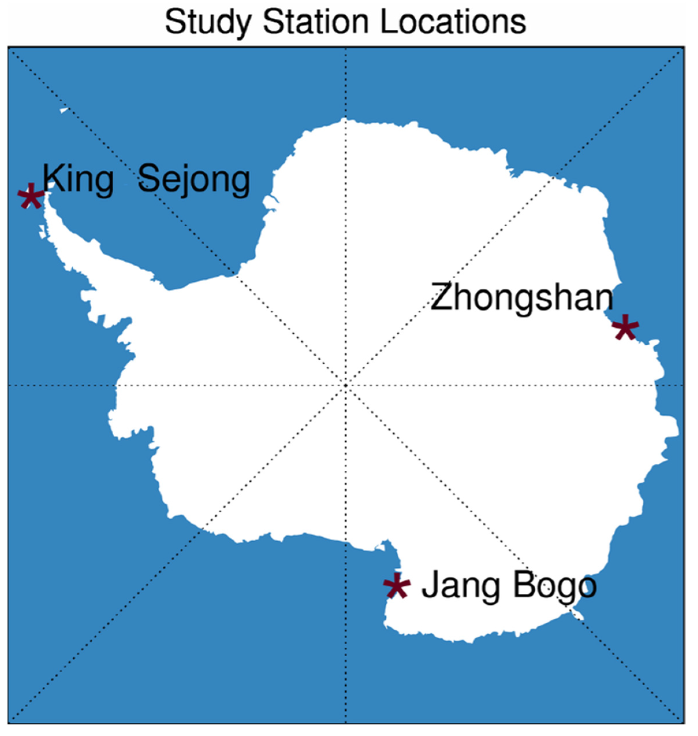
Figure 1. Three Antarctic TOC observation stations used in this study: King Sejong station on King George island (58.47°W, 62.13°S); Jang Bogo station adjacent to the Ross Sea (164.23°E, 74.62°S); and Zhongshan station adjacent to the Indian ocean (76.22°E, 69.22°S).
Remotesensing 13 01594 g001
Figure 2. Comparison for the Level 2 pixel sizes of five satellites over the King Sejong station: GOME-2 (green); OMPS and AIRS (yellow) which has same Level 2 pixel size; OMI (purple); and TROPOMI (red).
Remotesensing 13 01594 g002
Figure 3. Scatterplots for the TOC comparison between satellite measurements and the Brewer measurements at the King Sejong station: (a) Level 2; and (b) Level 3 TOC comparisons.
Remotesensing 13 01594 g003
Figure 4. Scatterplots for the TOC comparison between satellite measurements and the Brewer measurements at the Jang Bogo station: (a) Level 2; and (b) Level 3 TOC comparisons.
Remotesensing 13 01594 g004
Figure 5. Scatterplots for the TOC comparison between satellite measurements and the Brewer measurements at the Zhongshan station: (a) Level 2; and (b) Level 3 TOC comparisons.
Remotesensing 13 01594 g005
Figure 6. Monthly separated comparison between AIRS Level 2 TOCs and TOCs from the Brewer and satellite measurement at the King Sejong (left); Jang Bogo (middle); and Zhongshan (right) stations. Each month has different color: September (blue); October (red); November (cyan); December (black); January (pink); and February (yellow).
Remotesensing 13 01594 g006
Figure 7. Spatial distribution of OMI (left) and OMPS (middle) monthly mean TOC over the Antarctic area during September (top); October (middle); and November (bottom) 2019. The difference of monthly mean TOCs between OMI and OMPS are also examined (right). Here, Level 3 TOCs are used.
Remotesensing 13 01594 g007
Table 1. Summary of Brewer specifications for each station used in this study.
StationLongitudeLatitudeInstrument ModelInstrument NumberData Representative
King Sejong58.47°W62.13°SMK IV122Both DS and ZS
Jang Bogo164.23°E74.62°SMK III148Both DS and ZS
Zhongshan76.22°E69.22°SMK IV (~2010)
MK III (2010~)
74
193
Either DS or ZS
Either DS or ZS
Table 2. The MBE (MABE) values for satellite data at each station (unit: DU). Since TROPOMI does not provide Level 3 data, the value does not exist, so all tables are marked with blanks.
StationMeasure Type Product LevelOMITROPOMIOMPSAIRSGOME-2
King SejongDS26.5 (10.9)3.4 (8.9)1.0 (13.0)10.5 (19.7)10.1 (13.7)
ZS25.3 (11.4)−0.7 (8.9)−2.4 (12.2)8.8 (20.1)6.1 (12.3)
DS37.8 (13.5) 6.8 (13.1)11.2 (23.0)9.7 (13.6)
ZS35.5 (13.1) 3.2 (11.4)9.1 (23.8)5.8 (12.6)
Jang BogoDS22.9 (6.8)−0.1 (6.4)−8.8 (15.6)−11.7 (21.0)2.8 (10.3)
ZS22.0 (6.0)0.4 (5.9)−7.0 (13.4)−8.8 (19.1)3.8 (9.2)
DS30.3 (6.7) 2.7 (6.5)−12.5 (18.4)1.0 (9.7)
ZS3-0.1 (6.6) 2.5 (6.6)−9.4 (16.8)1.5 (8.1)
ZhongshanDS21.2 (6.1)8.6 (9.5)−8.5 (15.9)−10.2 (21.7)3.3 (10.7)
ZS2−7.7 (14.5)8.0 (9.5)−24.0 (25.4)−16.0 (30.9)−8.2 (14.3)
DS30.3 (5.9) 3.0 (6.9)−12.2 (19.4)3.4 (7.95)
ZS3−9.5 (16.1) −14.2 (17.4)−22.3 (31.1)1.0 (6.9)
Table 3. The RMSE values for satellite data at each station (unit: DU).
StationMeasure TypeProduct LevelOMITROPOMIOMPSAIRSGOME-2
King SejongDS215.412.517.626.217.4
ZS215.311.616.526.816.4
DS318.4 17.733.821.6
ZS317.4 14.532.021.5
Jang BogoDS211.19.023.729.715.1
ZS28.07.525.629.720.1
DS313.0 12.227.414.8
ZS319.8 19.429.221.0
ZhongshanDS210.013.320.930.714.6
ZS218.112.030.144.318.1
DS39.6 10.330.611.3
ZS319.8 22.446.68.6
Table 4. The number of data used only when comparing data that exist at the same time among all data calculated at each station.
StationMeasure TypeProduct LevelOMITROPOMIOMPSAIRSGOME-2
King SejongDS2466159375785629
ZS2110731676616901206
DS3696 373865486
ZS31599 7582002909
Jang BogoDS2164195345349332
ZS2246199449448432
DS3327 327343276
ZS3428 428442362
ZhongshanDS21376165107519401159
ZS215087121370
DS31678 10722064893
ZS3184 7125939
Publisher’s Note: MDPI stays neutral with regard to jurisdictional claims in published maps and institutional affiliations.

