
Estimating Aboveground Biomass Using Sentinel-2 MSI Data and Ensemble Algorithms for Grassland in the Shengjin Lake Wetland, China


1
School of Resources and Environmental Engineering, Anhui University, Hefei 230601, China
2
Anhui Province Key Laboratory of Wetland Ecosystem Protection and Restoration (Anhui University), Hefei 230601, China
3
Management Bureau of Anhui Shengjin Lake National Nature Reserve, Chizhou 247210, China
*
Author to whom correspondence should be addressed.
Remote Sens. 2021, 13(8), 1595; https://0-doi-org.brum.beds.ac.uk/10.3390/rs13081595
Submission received: 11 March 2021
/
Revised: 9 April 2021
/
Accepted: 13 April 2021
/
Published: 20 April 2021
(This article belongs to the Section Ecological Remote Sensing)
Abstract
:Wetland vegetation aboveground biomass (AGB) directly indicates wetland ecosystem health and is critical for water purification, carbon cycle, and biodiversity conservation. Accurate AGB estimation is essential for the monitoring and supervision of ecosystems, especially in seasonal floodplain wetlands. This paper explored the capability of spectral and texture features from the Sentinel-2 Multispectral Instrument (MSI) for modeling grassland AGB using random forest (RF) and extreme gradient boosting (XGBoost) algorithms in Shengjin Lake wetland (a Ramsar site). We use five-fold cross-validation to verify the model effectiveness. The results indicated that the RF and XGBoost models had a robust and efficient performance (with root mean square error (RMSE) of 126.571 g·m−2 and R2 of 0.844 for RF, RMSE of 112.425 g·m−2 and R2 of 0.869 for XGBoost), and the XGBoost models, by contrast, performed better. Both traditional and red-edge vegetation indices (VIs) obtained satisfactory results of AGB estimation (RMSE = 127.936 g·m−2, RMSE = 125.879 g·m−2 in XGBoost models, respectively), with the red-edge VIs contributed more to the AGB models. Moreover, we selected eight gray-level co-occurrence matrix (GLCM) textures calculated by four processing window sizes using the mean value of four offsets, and further analyzed the results of three analysis sets. Textures derived from traditional and red-edge bands using a 7 × 7 window size performed better in biomass estimation. This finding suggested that textures derived from the traditional bands were as important as the red-edge bands. The introduction of textures moderately improved the accuracy of modeling AGB, whereas the use of textures alo ne was not satisfactory. This research demonstrated that using the Sentinel-2 MSI and the two ensemble algorithms is an effective method for long-term dynamic monitoring and assessment of grass AGB in seasonal floodplain wetlands, which can support sustainable management and carbon accounting of wetland ecosystems.
1. Introduction
Wetlands are often transitional regions between terrestrial and aquatic ecosystems and serve extensive ecosystem functions, such as flooding and erosion reduction, ecological purification and protection, biodiversity conservation, and carbon storage [1,2,3]. Vegetation is a key component of wetland ecosystems and thus contributes to maintain ecosystem structure and function [4,5]. The biomass of wetland vegetation excellently indicates ecosystem health and has great significance in the global carbon cycle as an important parameter for evaluating the carbon sequestration capacity of wetlands [6,7]. Regional vegetation biomass changes are related to wetland ecosystem functional characteristics and carbon balance [8,9]. Accurate estimating for vegetation biomass is the basis of studying material circulation, energy flow, and bio-productivity. This allows a better understanding of the spatial temporal dynamics of wetland ecosystems and provides basic information for evaluating wetland ecological status and managing wetland natural resources sustainably [9,10,11], especially in floodplain wetlands where seasonal water level altering often result in potential variations in vegetation growth and distribution [12]. Therefore, the rapid and efficient biomass estimation of wetland vegetation, especially aboveground biomass (AGB), at a regional scale is required [13].
Traditionally, methods of vegetation biomass assessment are based on field surveying and these are very accurate which can be used for remote sensing-based AGB modeling. However, they are often time consuming and labor intensive in large-scale studying areas as wetlands have poor accessibility, especially in their core area [4,10]. Thus, traditional surveying methods are distinctly limited in both spatial and temporal scales [14]. Conversely, remote sensing technology, combined with a few field surveys in representative zones can realize rapid, dynamic, and regional-scale monitoring for AGB of dominant wetland vegetation [5,10,15,16]. Remote sensing images have become the efficient data sources of AGB estimation [8]. However, there are still challenges in selecting the appropriate remote sensing data, variables, and modeling algorithms for different ecological environments. Active remote sensing like light detection and ranging (LiDAR) and synthetic aperture radar (SAR) have various advantages [17,18]. Microwave-based SAR can determine the moisture content and canopy structure of vegetation as it can penetrate through clouds and vegetation. SAR is more suitable the inversion of vegetation parameters with evident structural characteristics. However, the saturation problem of the SAR backscattering coefficient in high biomass areas reduces the AGB modeling accuracy in wetlands [19]. LiDAR has incomparable advantages in acquiring objects’ horizontal and vertical information [20], which has been applied successfully for wetland biomass estimation, especially for mangroves in coastal intertidal zones [21]. Nevertheless, the application of LiDAR data is restricted in wetlands due to limited spatial and temporal coverage. LiDAR is also quite costly and lacks spectral information. Optical sensors remain one of the most interesting options for biomass estimation as newer sensors with finer spatial and temporal resolutions, as well as richer spectral information, have become available. Generally, biomass estimation using optical sensor data is based on vegetation indices (VIs), like difference vegetation index (DVI) [22], enhanced vegetation index (EVI) [23], and normalized difference vegetation index (NDVI) [24]. However, using conventional VIs for AGB estimation has limited success for areas with high-density vegetation [4]. Seasonal wetlands in the Yangtze River floodplain are characterized by grass species with high levels of productivity. Therefore, conventional vegetation indices predict biomass with limited precision in wetlands.
Texture provides the image information on the horizontal structure, spatial variation, and relativity of gray values, that help users identify ground objects or regions of interest in images [25,26]. The approaches to texture measure mainly include four categories: statistical, structural, model-based and transform-based methods [27]. The statistical methods can effectively describe the texture and are regarded as one of the earliest methods of image texture analysis [28,29]. The statistical methods are based on the spatial distribution of image gray levels, include gray-level co-occurrence matrix (GLCM), local binary pattern (LBP), autocorrelation function (ACF), and sum and difference histograms (SADH) [29,30]. As a statistical analysis method, the popular GLCM textures have strong adaptability and robustness, which were considered as efficient and promising technique for texture analysis [25,31]. Textures were considered as a solution to the problem of vegetation index saturation in dense biomass areas, and can be widely applied to remote sensing imagery, which may be an effective approach for improving the accuracy of modeling biomass at local and regional scales. Many studies have applied textures in biomass estimation using optical sensors or SAR data, mainly for forests [26,30,31,32,33,34]. Texture analysis is more effective in images with higher spatial resolution as finer structural details can be distinguished [33]. Thus, there is great potential to improve AGB estimation by integrating textures with red-edge bands. However, texture is a complex property that is greatly influenced by study objects and topographic conditions, as well as the processing window size [35,36]. Therefore, although textures have great potential in estimating AGB, relevant studies involving wetland vegetation are inadequate.
The emergence of newer generations of medium-resolution multispectral sensors such as those carried by Sentinel-2 series satellites provide new opportunities for grassland vegetation biomass estimation in wetlands. Moreover, data from Sentinel-2 satellites have been made freely available by the European Space Agency (ESA). The Sentinel-2 mission has two complementary satellites with a five-day revisiting period. The Sentinel-2 are multi-spectral imaging sensors, each carrying a multi-spectral instrument with 13 spectral bands including visible, near infrared (NIR), and short-wave infrared at fine spatial resolution (10, 20, and 60 m). Significantly, Sentinel-2 is the only multispectral sensor mission with four strategically positioned bands with 20 m spatial resolution in the red-edge region, namely bands 5, 6, 7 and 8A (705 to 865 nm) [37]. These red-edge bands are strongly effective for monitoring vegetation and can quantify grass AGB as well as map vegetation communities inside wetlands [38,39]. The Sentinel-2 sensors also provide finer spatial resolution, which may be more suitable for monitoring wetland AGB at a regional scale, compared to the Landsat TM. However, although images from Sentinel-2 have a higher spatial–temporal resolution and richer spectral information, data mining for wetland vegetation biomass deserves more attention, especially with the red-edge bands and its derivatives.
Recently, machine learning techniques, like artificial neural network (ANN), support vector regression (SVR), and decision tree have been more frequently applied in biomass estimation in integration of remote sensing data and sample surveying data [40,41,42,43]. Non-parametric models for AGB estimation with machine learning algorithms have been proved to be better than parametric models with linear algorithms in describing the nonlinear relationship between measured biomass and remote sensing-based variables [19,44]. Ensemble learning is a very popular and effective machine learning method, because of the improvement of the generalization ability and robustness by modeling and combining multiple base learners. Bagging and boosting are two typical and popular ensemble approaches. Random forest (RF), a classical bagging algorithm, is known as one of the best machine learning algorithms [45]. Some studies have also demonstrated that RF performed well in AGB estimation [5,46,47,48], because of its robustness and processing ability for high-dimensional features [49]. Another advantage of the RF algorithm is the evaluation of variable importance. The extreme gradient boosting (XGBoost), one of the boosting methods, is efficient and flexible to solve the regression, classification and ranking problems, thus has been widely recognized in machine learning and Kaggle competitions, especially for structured or tabular data [50]. However, there are few studies on XGBoost in biomass estimation, especially in estimating wetland grassland AGB. The selection of an optimal subset of variables can improve the performance of modeling AGB and contribute to understand the models [51]. Moreover, variable selection can reduce dimension and avoid overfitting of the model.
Shengjin Lake is a representative river-connected and seasonally shallow lake in the middle and lower Yangtze River floodplain in China. When the lake enters the dry season, it exposes a wide area of grassland and marshland which provide precious habitats and food for large number of wintering waterbirds (e.g., Grus monacha, Ciconia boyciana); thus, it was designated as a Ramsar site in 2015. Therefore, it has important practical significance to study the grassland AGB in the Shengjin Lake wetland. This study integrated Sentinel-2 MSI images and field biomass data for modeling grassland AGB using RF and XGBoost algorithms in Shengjin Lake wetland. Specifically, we: (i) explored the capability of Sentinel-2 images to estimate grassland AGB at Shengjin Lake using RF and XGBoost models respectively, (ii) compared the performance of Sentinel-2-based different variable combinations, as well as GLCM textures on different window sizes for modeling AGB, and (iii) compared the effect of variable selection on the RF and XGBoost models for AGB estimation.
2. Materials and Methods
2.1. Study Area
This study executed field surveys in the core area of the Anhui Shengjin Lake National Nature Reserve (30°15′–30°30′N, 116°55′–117°15′E, Figure 1). The lake is naturally divided into three connected water surfaces from south to north (upper, middle, and lower lake). The main source of incoming water for the lake comes from two tributaries (Zhangxi and Tangtian Rivers) and runs to the Yangtze River via the Huangpen sluice. Shengjin Lake belongs to subtropical monsoon climate region. This region has an annual average temperature of about 16.1 °C and abundant rainfall, averaging approximately 1600 mm annually. It is a typical seasonal and river-connected lake with a significant seasonal fluctuation in water levels. During the lake’s July–August wet season, the water level reaches its highest point of the year, and the lake area grows up to 138 km2. While as the advent of the drought period (October to the following March), the lake level has a sharp drop, leads to the area of the lake falling as low as 34 km2, exposing a wide range of tidal flats and grasslands, especially in the upper and lower lake. The distribution of the grassland, which is dependent on water level fluctuation, is characterized by irregular concentric rings along a moisture gradient with lower vegetation density closer to the lake shoreline. The grassland is mainly covered by three types of plants (Carex thunbergii, Carex cinerascens, and Polygonum criopolitanum). The Shengjin Lake wetland is an important wintering ground and migratory stopover for waterbirds and is designated as a Ramsar site.
2.2. Field Biomass Data
The grassland-growing period of the Shengjin Lake wetland is divided into spring and autumn. For the present study, field sampling was conducted from 8 to 13 November 2019, during the peak grass growing period. According to the distribution and growing trends of the grasslands, 78 sampling quadrats were set in the upper and lower lakes, the sample plots, namely, A, B and C, contain 24, 33, 21 quadrats respectively (Figure 1). The plants in the sample quadrats were mainly Cyperaceae with a small area of Polygonaceae. The quadrat size was 0.5 × 0.5 m, and the distance between sampling quadrats was 30–100 m to ensure that the main vegetation communities were covered. For each quadrat, we recorded detailed geographic coordinates and elevation information via a Garmin global positioning satellite (GPS) system and then identified the vegetation type and harvested all aboveground vegetation within the quadrat. After removing dead materials from clipped plants, we obtained the mean fresh AGB by weighing three times, as the observed biomass values.
2.3. Sentinel-2 Data Processing and Variables
In this study, we utilized the Sentinel-2A MSI Level-1C (L1C) products collected from the USGS Earth Explorer (https://earthexplorer.usgs.gov/, accessed on 11 March 2021). Considering cloud cover of images and field sampling date, two Sentinel-2A MSI images were obtained on 8 November 2019. The L1C product is an image of top-of-atmosphere (TOA) reflectance after ortho-rectification and geometric corrections at sub-pixel accuracy. Sentinel-2A MSI data have rich spectral information covering 13 bands including visible, near-infrared, red-edge, and shortwave infrared wavelengths with different spatial resolutions. This study selected 10 bands of Sentinel-2A MSI, excluding bands 1, 9, and 10, as they mainly relate to atmosphere and water elements (Table 1). The Sentinel-2A L1C ortho-rectified images were processed into orthoimage bottom-of-atmosphere (BOA) corrected reflectance products by the third-party plug-in Sen2Cor version 2.8 provided by ESA and then resampled from the 20 m resolution to 10 m of Sentinel-2A bands by ESA’s SNAP version 7.0.
To study the potential and characteristics of Sentinel-2 MSI for grassland AGB estimation in wetlands, we selected raw bands, VIs, and textures as input variables. For this paper, 20 VIs were finally chosen according to preliminary comparative analysis and relevant studies [16,38,46,52]. Ten conventional VIs were extracted from Sentinel-2A bands (band 2, 3, 4, 8, 11, 12). The near-infrared and red-edge bands are significant for monitoring wetland vegetation and the VIs of these bands showed strong correlations with biomass [4,46]. Thus, we selected 10 red-edge VIs as a special type of input variables owing to the availability of the three red-edge (band 5, 6, 7). It presents a detailed properties and corresponding equations for the VIs in the paper (Table 1).
Texture analysis based on the GLCM technique [25], which has strong adaptability and robustness, thus enjoy wide popularity. In this study, we derived the texture variables from Sentinel-2 MSI bands via the GLCM-based co-occurrence measures tool in ENVI 5.3 version. Eight frequently used texture metrics, namely, mean, variance, homogeneity, contrast, dissimilarity, entropy, second moment, and correlation were selected (Table 1), because they have already been proven to be effective for estimating AGB [26,33,42,43]. Proper window size selection is a critical factor in texture analysis. Smaller windows may exaggerate variations and increase the pixel noise, whereas larger windows may miss important information [26,30]. Therefore, to determine the optimal window size for accurate AGB estimation, we selected window sizes with high correlations between texture-estimated and observed AGB by referring to a previous study [26]. Textures were calculated on four different processing window sizes (3 × 3, 5 × 5, 7 × 7, and 9 × 9 pixels) at 64-bit gray-level quantization and a relative displacement vector (d, θ), which represents direction and displacement parameters, respectively. The co-occurrence shift (d) was set to 1 after compared the performance of other shifts in the models. In order to reduce the effects of direction parameters and the dimensions of input variables on modeling, the mean of the four directions (θ = 0°, 45°, 90°, 135°) for each texture calculation was selected, which are expressed in Cartesian coordinates as [1, 0], [1, 1], [0, 1], and [1, −1]. Considering Sentinel-2 MSI’s unique red-edge bands, we designed three analysis sets for each processing window size to further compare the performance between traditional and red-edge bands for predicting AGB. Analysis set 1 contains 48 input texture variables generated by only the ordinary bands (including band 2, 3, 4, 8, 11, 12). Analysis set 2 contains 32 input texture variables generated by only the red-edge bands (including band 5, 6, 7, 8A). Analysis set 3 includes both of the above.

Table 1.
Description and formula of input variables, including raw bands, traditional and red-edge vegetation indices, and textures, derived from Sentinel-2A MSI for modeling AGB in this study.
Table 1.
Description and formula of input variables, including raw bands, traditional and red-edge vegetation indices, and textures, derived from Sentinel-2A MSI for modeling AGB in this study.
| Variables | Equation | References | |
|---|---|---|---|
| Original spectral bands | |||
| Blue | B2 | 10 m | [53] |
| Green | B3 | 10 m | |
| Red | B4 | 10 m | |
| Red edge 1 | B5 | 20 m | |
| Red edge 2 | B6 | 20 m | |
| Red edge 3 | B7 | 20 m | |
| NIR | B8 | 10 m | |
| NIR narrow | B8A | 20 m | |
| SWIR | B11 | 20 m | |
| SWIR | B12 | 20 m | |
| Traditional spectral indices | |||
| ARVI | [54] | ||
| CIg | [55] | ||
| DVI | [56] | ||
| EVI | [57] | ||
| GNDVI | [58] | ||
| MSAVI | [59] | ||
| NDII | [60] | ||
| NDVI | [61] | ||
| SR | [62] | ||
| VARIg | [63] | ||
| Red-edge spectral indices | |||
| CIre | [64] | ||
| IRECI | [65] | ||
| MCARI | [66] | ||
| NDVIre1 | [67] | ||
| NDVIre2 | [68] | ||
| NDVIre3 | [68] | ||
| NDre1 | [67] | ||
| NDre2 | [69] | ||
| SRre | [70] | ||
| S2REP | [65] | ||
| Gray-level co-occurrence matrix (GLCM) | |||
| Mean (MEA) | [25] | ||
| Variance (VAR) | |||
| Homogeneity (HOM) | |||
| Contrast (CON) | |||
| Dissimilarity (DIS) | |||
| Entropy (ENT) | |||
| Second Moment (ASM) | |||
| Correlation (COR) | |||
ARVI: Atmospherically Resistant Vegetation Index; CIg: Green Chlorophyll Index; DVI: Difference Vegetation Index; EVI: Enhanced Vegetation Index; GNDVI: Green Normalized Difference Vegetation Index; MSAVI: Modified Soil Adjusted Vegetation Index; NDII: Normalized Difference Infrared Index; NDVI: Normalized Difference Vegetation Index; SR: Simple Ratio; VARIg: Visible Atmospherically Resistant Index green; Cire: Chlorophyll Index red-edge; IRECI: Inverted Red-edge Chlorophyll Index; MCARI: Modified Chlorophyll Absorption Ratio Index; NDVIre1: Normalized Difference Vegetation Index Red-edge 1; NDVIre2: Normalized Difference Vegetation Index Red-edge 2; NDVIre3: Normalized Difference Vegetation Index Red-edge 3; NDre1: Normalized Difference Red-edge 1; NDre2: Normalized Difference Red-edge 2; SRre: Simple Ratio Red-edge; S2REP: Sentinel-2 Red Edge Position.
2.4. Algorithms of Modeling AGB
The random forest (RF) algorithm, developed by Breiman, is an efficient bagging-based ensemble learning method for improving the regression and classification tree by combining multiple decision trees [71]. For each decision tree in RF modeling, we utilized bootstrapping method (random sampling with replacement) to select the original data set. Two-thirds of the data set was used to generate trees without pruning, the remaining third (out-of-bag (OOB) data), as internal validation sets, was used for calculating the OOB error [72]. The RF algorithm employs two methods for assessing predictor variable importance, %IncMSE and IncNodePurity. In the present study, we selected the first metric, which is to measure the decrease in accuracy on randomly permuting OOB data, because it was used in many studies [44]. A higher %IncMSE value indicates that the modeling variable is more important. Two important parameters must be optimized in the RF models: (i) ntree, the tree number contained in the RF model, and (ii) mtry, the variable number used during node splitting of each tree. We used grid-search approach with 5-fold cross-validation in term of root mean square error (RMSE) to adjust hyperparameters for more robust models. In our study, the optimal values of ntree are 500, and mtry ranged from 5 to 28 for the three analysis sets. In addition, the node sizes of all RF models were selected as the default value of 1.
XGBoost is an advanced ensemble learning algorithm based on the Gradient Boosting framework, which was developed by Chen et al [50]. This algorithm is, essentially, an improved gradient boosting decision tree (GBDT). Compared to GBDT, XGBoost performs well in avoiding overfitting and simplifying models by introducing regularization term into the objective function. Moreover, it applies the second-order Taylor expansion to the objective function and utilizes the first-order and second-order derivative at the same time for the faster and more accurate gradient descent of the model [44]. XGBoost has three common methods of evaluating feature importance, Gain, Weight and Cover. The first measure was used in this study, which is computing the mean gain of each feature used as split node across all trees [50]. The XGBoost hyperparameters can be divided into three groups: general, booster and learning task parameters. We also used grid-search approach with 5-fold cross-validation in term of RMSE values to tune the hyperparameters of the XGBoost models.
To investigate the effect and importance of different feature variables for modeling grass AGB in wetlands, we implemented four RF and XGBoost models with different combinations of variables: (i) raw bands + textures, (ii) raw bands + traditional VIs, (iii) raw bands + red-edge VIs, and (iv) raw bands + textures + traditional and red-edge VIs. It should be noted that this study constructed the RF and XGBoost models using the scikit-learn package in Python 3 (http://scikit-learn.org/stable/, accessed on 11 March 2021) [73].
2.5. Model Assessment
A total of 78 sampling biomass values were randomly divided into two subsets: 70% was used for the training data set for model learning and the remaining 30 percent as the testing set of rating. Cross-validation was applied to assess the generalization capability of the model when there is an inadequate number of sample points. In addition, we selected three criteria for evaluating the RF model effectiveness, namely, the RMSE (Formula (1)), the coefficient of determination (R2, Formula (2)), and the coefficient of variation of the root mean square error (CV-RMSE, Formula (3)). These were calculated using five-fold cross-validation. Generally, the higher R2 and the lower RMSE and CV-RMSE represents, the model fits better.
where , represents the field measured and estimated AGB values in the ith sample respectively, is the measured AGB averaged over all samples, and n represents the size of the samples in different data set.
3. Results
3.1. AGB Models Based on Image Textures
To determine the optimal Sentinel-2 imagery-based texture for estimating AGB for wetland grasslands, a comparative analysis of GLCM-based textures using three analysis sets and four window sizes with RF and XGBoost regression algorithms was summarized in Table 2. For the RF models, the results showed that textures calculated on a 3 × 3 window size for different analysis sets performed worst in AGB estimation according to the five-fold cross-validated of RMSE, R2, and CV-RMSE values. As observed from the other window sizes for different analysis sets, the RF models have more or less similar accuracy. On the other hand, when using XGBoost algorithm, these results suggested that all models of textures calculated on a 7 × 7 window size for different analysis sets performed best for estimating AGB with the lowest RMSE, CV-RMSE, and the highest R2 values. For the analysis set 3 (including both traditional and red-edge band texture variables), all XGBoost models of different window sizes yielded the best performance when compared to the other analysis sets, and it was found the highest accuracy for 7 × 7 window size, with an RMSE of 127.578 g·m−2, R2 of 0.849, and CV-RMSE of 0.133. Surprisingly, compared to the analysis set 1 (only including traditional band textures), the performance of XGBoost models for the analysis set 2 (only the red-edge textures) was poorer for 5 × 5, 7 × 7 and 9 × 9 window sizes. Moreover, for the 5 × 5 and 7 × 7 window sizes, the AGB models of the analysis set 3 performed strongly when compared to the 3 × 3 and 9 × 9 window sizes. Therefore, the integration of red-edge and traditional textures on a 7 × 7 window size was selected for further analysis in this study.
3.2. Variable Combinations for Modeling AGB
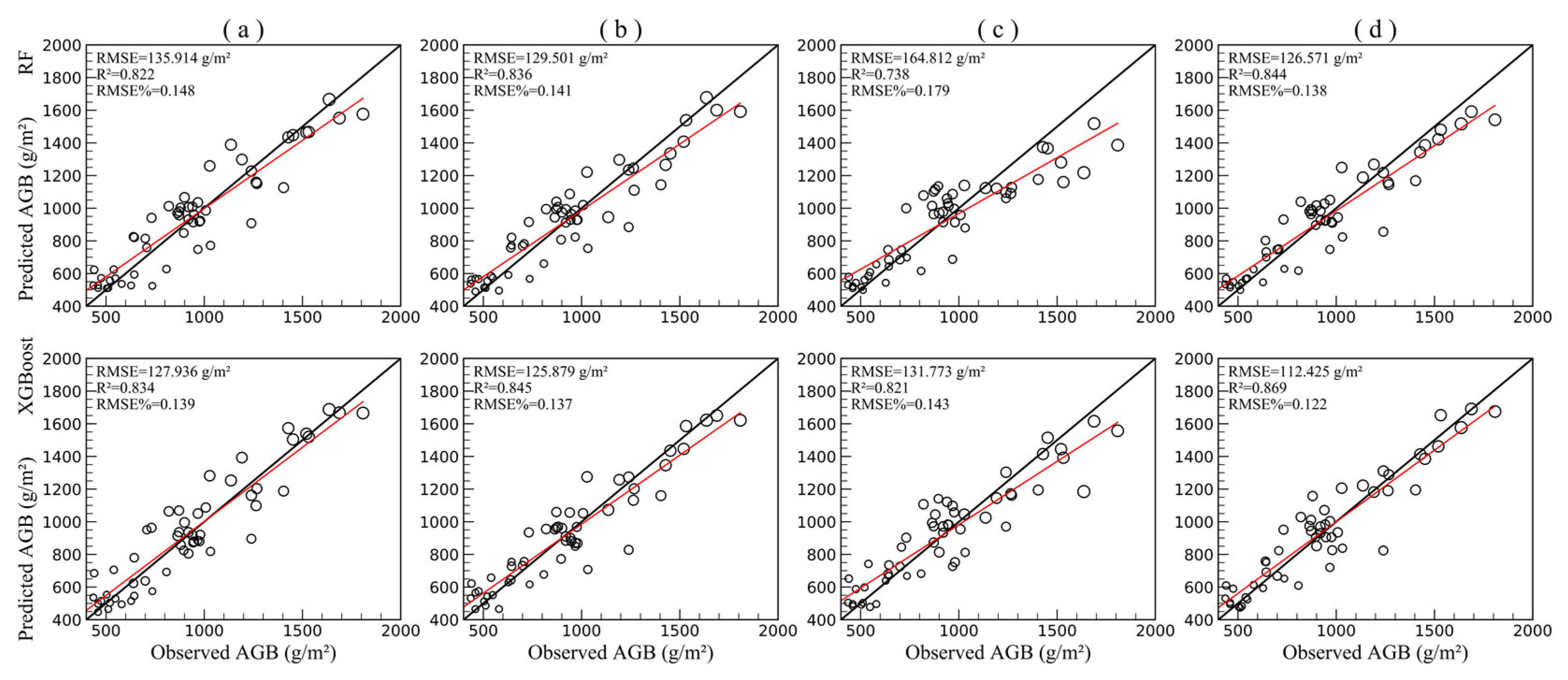
We repeatedly ran the RF and XGBoost models to optimize the values of hyperparameter according to the minimum RMSE values after five-fold cross-validation. The results presented statistical description for four AGB estimating models using the RF and XGBoost algorithms in Table 3. Obviously, these results suggested that the performance of estimating AGB using XGBoost algorithm was better than that of RF algorithm. In addition, Model 4 performed best with the highest accuracy for AGB estimation, producing the lowest RMSE and the highest R2 whether using RF model (R2 = 0.844, RMSE = 126.571 g·m−2) or XGBoost model (R2 = 0.869, RMSE = 112.425 g·m−2). When only red-edge vegetation indices and spectral bands were used as in Model 2, it achieved the second-best performance, whereas the values of R2 and RMSE of the Model 1 were 0.836, 129.501 g·m−2 for RF and 0.845, 125.879 g·m−2 for XGBoost respectively. These results indicated that the red-edge indices (Model 2) had a stronger advantage in biomass estimation than the traditional vegetation indices (Model 1). Model 3 (both RF and XGBoost algorithms) yielded the worst performance compared to the other models. Thus, the combination of all variables was applied to AGB estimation in this study area.
The relationships between observed and predicted biomass using various RF and XGBoost models were further analyzed and were shown as scatterplots in Figure 2. The results showed that Model 4 fitted better compared to the other models whether RF or XGBoost models. For all RF and XGBoost models, there were saturation problems, which indicated AGB underestimation in the high-biomass area. However, it was obvious that the use of XGBoost algorithm for estimating high biomass was stronger than the RF algorithm (more than 1300 g·m−2 for Model 4). Moreover, adding textures had positive effects on solving overestimate or underestimate problem for wetland AGB estimation, but using textures alone was not adequate. Overall, the mixture of bands, traditional and red-edge VIs, and textures resulted in the optimum variable combination for AGB estimation of wetland vegetation.
3.3. Variable Importance and Selection
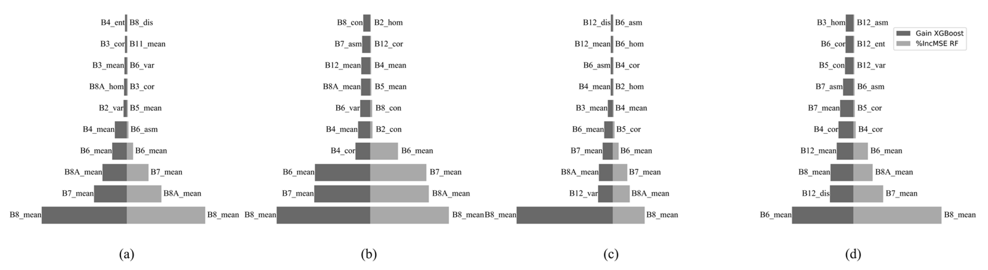
In this study, we utilized RF and XGBoost regression algorithm for the analysis set 3 to rank the texture variable importance of the models, based on %IncMSE and Gain respectively, and the top 10 textures of four different window sizes were shown in Figure 3. The results showed that the ranking of variable importance is not completely consistent, whereas all models included mean and correlation textures, which indicated that they correlated highly with AGB. The findings in our study were consistent with some previous studies, although those studies used different optical remote sensing data [26,44]. Moreover, the mean texture B8_mean, B7_mean, B8A_mean, and B6_mean appeared in the top 10 of all models ranking.
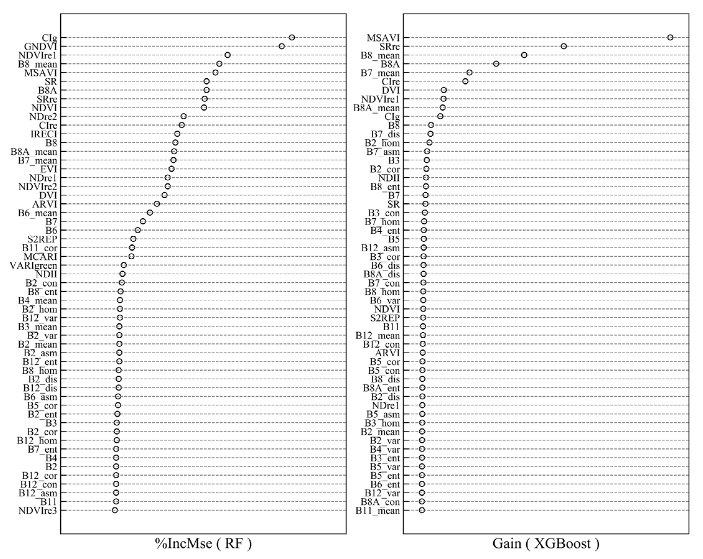
The relative importance of the input variables for Model 4 was determined using RF and XGBoost models. Figure 4 displayed the first half of the variable importance ranking (n = 55), which were measured by the decrease in %IncMSE and Gain respectively. The variable importance ranking of the RF model differed with that of the XGBoost model, but it was worth noting that SRre, NDVIre1, and MSAVI were important variables of both RF and XGBoost models, and the red-edge NDVI (NDVIre1) correlated strongly with biomass as compared with traditional NDVI. In addition, red-edge bands (B6, B7) and near-infrared bands (B8, B8A) had high importance for models than other bands. For GLCM textures, the mean of textures derived from Sentinel-2 imagery was one of the most important variables, namely, B8_mean, B7_mean, and B8A_mean.
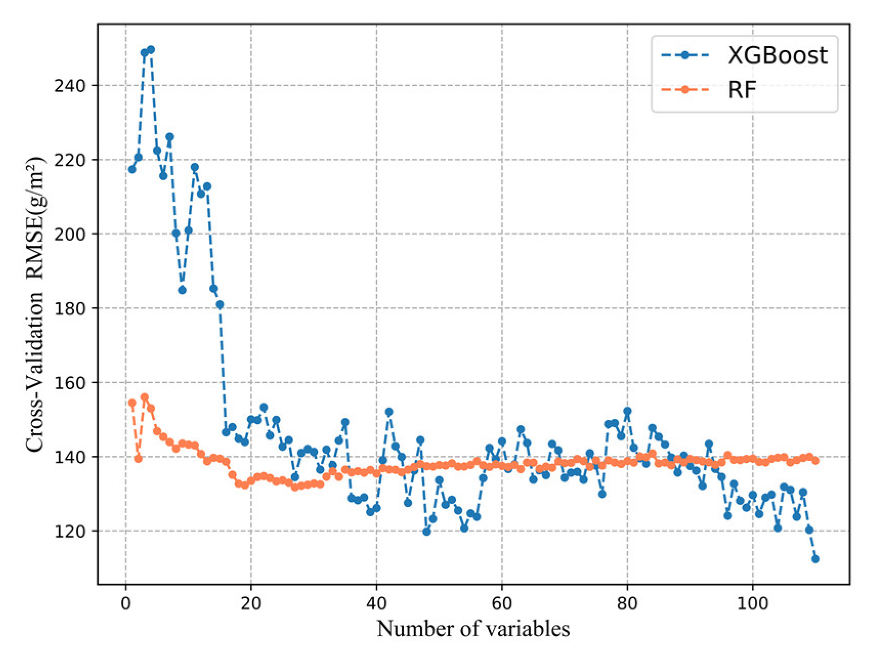
Furthermore, this study used recursive feature elimination (RFE) method with cross-validation to optimize the subset of predictor variables in Model 4. The results showed that the RMSE values of RF and XGBoost models slightly increased or decreased with feature elimination, as shown in Figure 5. Comparing the two models, the performance of XGBoost model was better than RF model, and the input variables had different effects on modeling performance. In addition, the number of input variables for XGBoost model affected relatively strongly performance when compared to the RF model. Finally, we selected the top 27 variables for the optimized RF model and all variables for the XGBoost model, as they provided the lowest RMSE values after five-fold cross-validation.
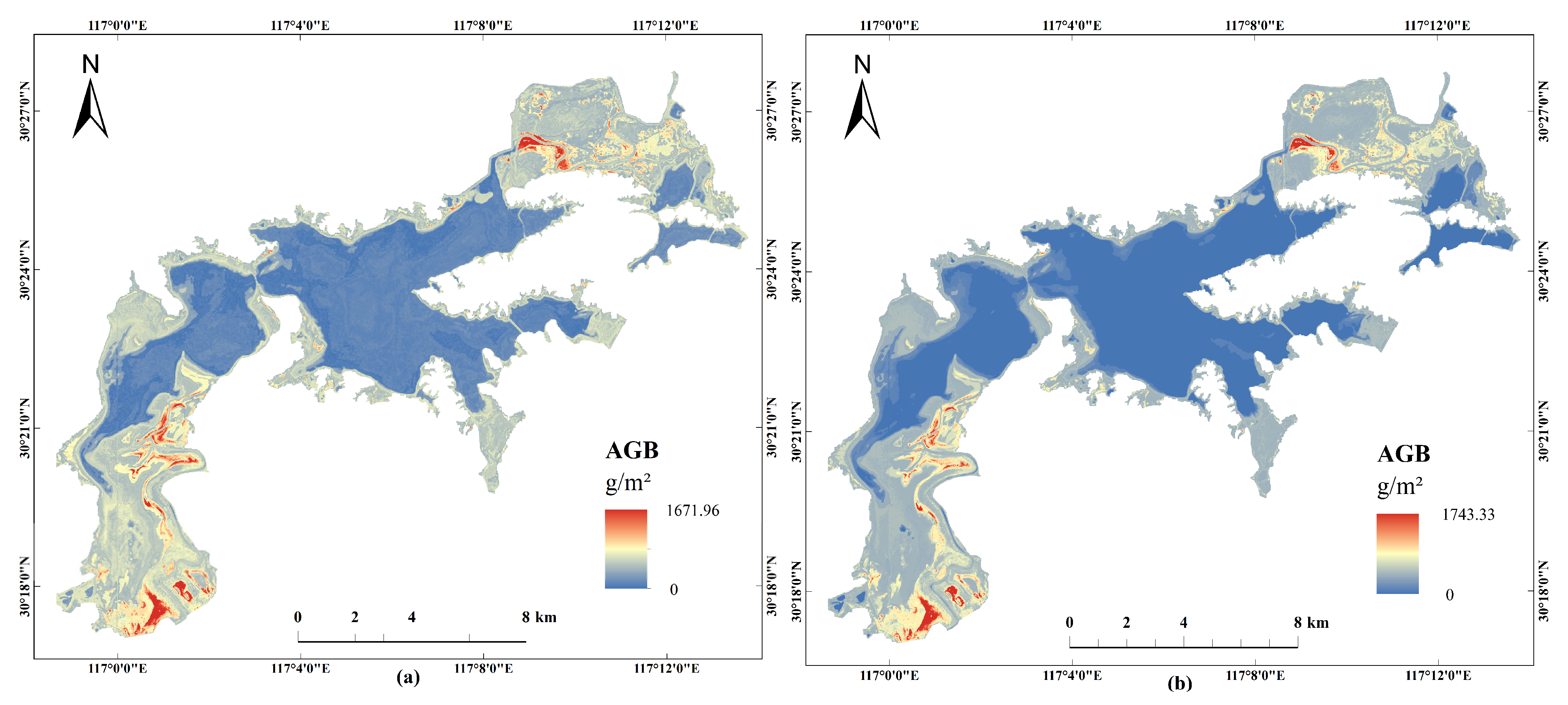
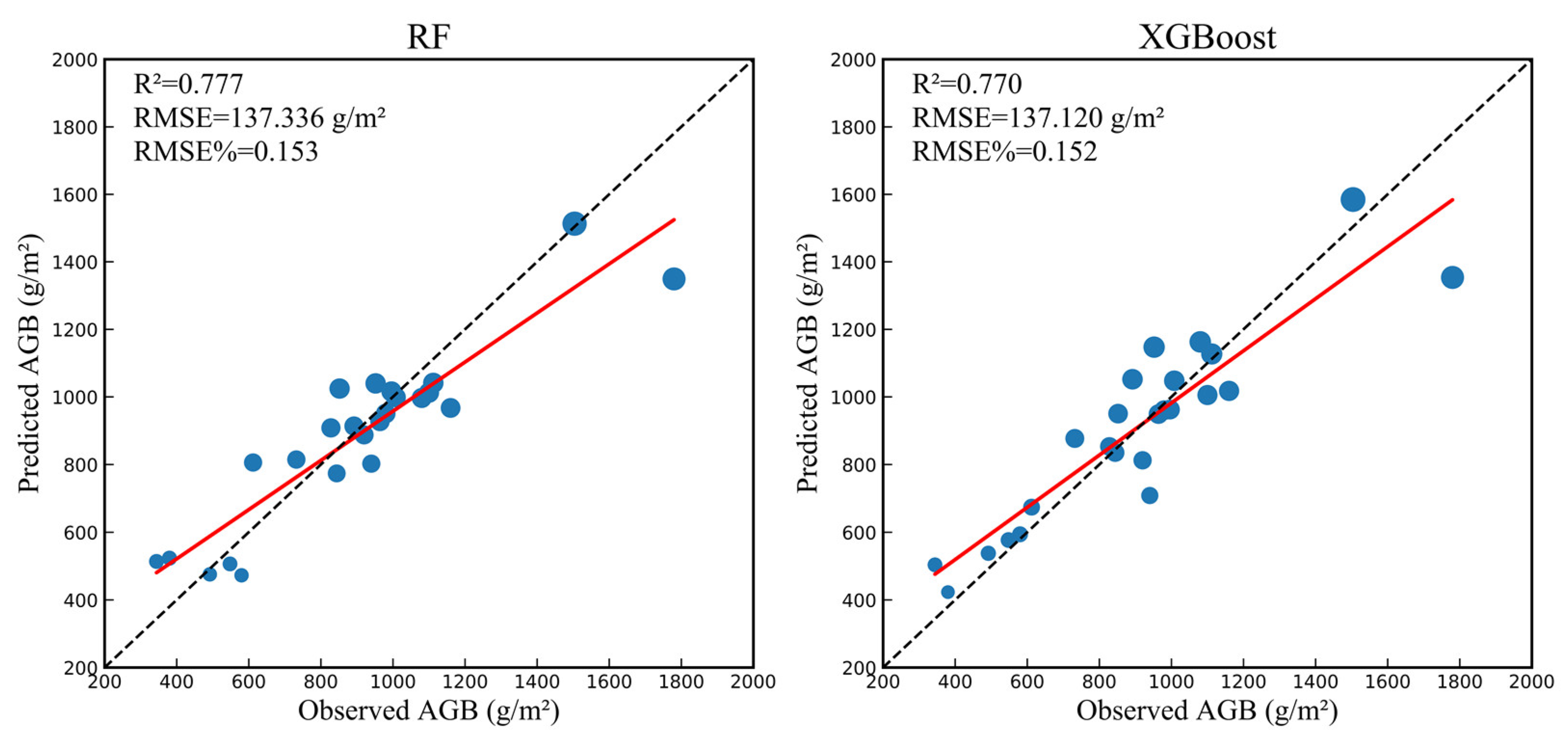
3.4. Spatial Pattern of AGB in the Shengjin Lake Wetland
In the paper, we utilized RF and XGBoost models with the optimized spectral and texture variables to map AGB in the Shengjin Lake wetland, respectively (Figure 6). The spatial distribution trends of the two AGB maps were similar. The AGB density value ranged from 0 to 1743.33 g·m−2 for XGBoost model, and 0 to 1671.96 g·m−2 for RF model. To validate the effectiveness of the RF and XGBoost models for estimating AGB, we used a testing data set of 24 sample quadrats to measure the model performance. The results showed plausible and strong explanatory statistical metrics for XGBoosot model (RMSE = 137.120 g·m−2, R2 = 0.770, CV-RMSE = 0.152), which was close to that for RF model (RMSE = 137.336 g·m−2, R2 = 0.777, CV-RMSE = 0.153) (Figure 7). The predicted AGB values were close to the observed AGB values in Figure 1. In conclusion, the lower AGB was overestimated, the higher AGB was underestimated. The XGBoost models performed better in solving underestimation and overestimation when compared to the RF models, whereas none of them can resolve the problems completely. The AGB map showed evident spatial heterogeneity; the higher AGB was mainly distributed in the upper and lower lake regions, and there was very sparse AGB distribution in the middle lake region.
4. Discussion
The application of remote sensing data in modeling herbaceous AGB in floodplain wetlands still faces some particular challenges due to species diversity, soil factors, and dense vegetation [4,74]. Although previous research achieved varying degrees of success by using optical sensors with various spatial and spectral resolution to estimate AGB in wetlands, the accuracies of these models were limited [8]. Previous studies have shown a saturation tendency when using traditional vegetation indices for AGB estimation in dense vegetation [8,46]. However, the new generation of medium-resolution optical sensors with strategically-positioned red-edge bands, like WorldView-2/3 and Sentinel-2, has effectively overcome this problem [34,48]. For example, Sibnada et al., investigated the performance of Sentinel-2 MSI and Landsat 8 OLI in grass AGB estimation under different fertilizer treatments, the results indicated that Sentinel-2 MSI performed better (R2 = 0.81, RMSE = 1.07 kg·m−2) compared with Landsat 8 OLI (R2 = 0.76, RMSE = 1.15 kg·m−2) [38]. Furthermore, previous study has found that the modeling accuracy of Sentinel-2 MSI (with 90.36% for bands, 85.54% for indices, and 88.61% for combined variables) and Worldview-2 (95.69%, 86.02%, and 87.09%) for distinguishing C3 and C4 grasses was comparable, and significantly better than that of Landsat 8 OLI (75.26%, 82.79%, and 82.79%), which demonstrated a great potential of new multispectral sensor with red-edge bands in grass species monitoring [37].
This study assessed the capacity of the Sentinel-2 MSI images in modeling grassland biomass using the RF and XGBoost models, respectively. The results showed acceptable accuracy of AGB estimation with an RMSE of 137.336 g·m−2 and R2 of 0.777 for RF and an RMSE of 137.120 g·m−2 and R2 of 0.770 for XGBoost. When compared with another study in a similar study area that using Landsat 8 OLI and RF algorithm for modeling grass biomass in the Poyang Lake wetland (R2 = 0.68, RMSE = 0.26 kg·m−2) [5], the results of using Sentinel-2 MSI were relatively better. Sentinel-2 MSI data are superior for estimating biomass than Landsat 8 OLI, which may be mainly attributed to higher resolution, unique red-edge bands and rich spectral information. These results demonstrated the potential of the strategically-positioned bands in strengthening the capability of the sensors for AGB estimation [75,76]. Additionally, some studies have proven that the availability of Sentinel-2 bandwidth and band position in vegetation monitoring [77]. These results pointed out that Sentinel-2 bands are more precise than that of Landsat 8 OLI or some other broadband sensors. Undoubtedly, the use of commercial hyperspectral data can provide much more vegetation spectral information than medium-resolution optical sensors, but this is greatly limited by its high cost, difficult availability, and complex processing [78]. Sentinel-2 MSI were obtained for free with an advanced open-source processing software (SNAP) and a professional user communication forum. The availability of Sentinel-2 data is critical to AGB estimation of wetland vegetation, especially in large scale areas. Overall, Sentinel-2 provides an effective alternative to low spatial resolution satellites or commercial sensors.
Some studies have demonstrated the effectiveness and robustness of VIs in estimating AGB [16,38,48], as they can decrease the effect of the background and environment on reflectivity [47]. However, the use of VIs to estimate vegetation AGB limited by saturation problems, especially in high density biomass areas [4,79]. Some studies have demonstrated that VIs derived from the NIR narrow and red-edge bands can yield higher accuracy of AGB estimation [46,79], and contribute to alleviate saturation problem [76]. In this paper, traditional and red-edge vegetation indices were used separately to model AGB, each producing satisfactory accuracy. It is a remarkable fact that the red-edge VIs performed better than those of the traditional, which is consistent with previous studies. Red-edge bands (B6, B7) and near-infrared bands (B8, B8A) had high importance of models in this study, which was similar to the results of Castillo et al. They found the Sentinel-2 red-edge (B6, B7) and near-infrared (B8, B8A) had a stronger correlation with AGB than visible and short-wave infrared bands, and the VIs from red-edge (B5, B6), NIR (B8) and SWIR (B12) correlated highly with AGB than combination of other bands [80]. This paper found SRre, NDVIre1 were the important variables for estimation biomass, previous studies have found similar results [46,48]. In addition, remote sensing data with finer spatial resolution and rich spectral information contribute to improving AGB modeling accuracy and overcoming saturation problems [19].
We also assessed the performance of Sentinel-2-based texture variables for modeling grassland AGB in wetlands. The results suggested the mixture of spectral and texture variables (on a 7 × 7 window size) improved accuracy in estimating AGB, which is consistent with other studies [34,42], whereas modeling performance with the use of textures alone to estimate AGB was relatively poor (Table 2). Some studies have found that the effect of texture and spectral variables on estimating forest AGB was greatly affected by stand structure, the models tended to choose spectral variables in forest with complex structure, and the textures are more important in the simple structure forest [18,44]. Wetland grassland presents high spatial and spectral variability as complex environmental gradients lead to short ecotones and obvious divisions between the vegetation units [4], which may limit textures in wetland AGB estimation. Moreover, this study found that the introduction of textures improved the modeling accuracy for AGB estimation. This result was consistent with previous studies, textures had a positive effect on biomass estimation [30,76].
Furthermore, this study investigated the accuracy of GLCM textures with different window sizes for AGB estimation (Table 2). The results indicated that the medium window sizes (5 × 5, 7 × 7) are more sensitive for estimating AGB than larger or smaller window sizes when using Sentinel-2 imagery, which is similar to previous studies [81]. In contrast, Dong et al. investigated GLCM textures with window sizes from 3 to 53 using Worldview-2 (a remote sensory data source with higher spatial resolution) and found that larger window sizes are potentially effective, and once the window size more than 43, the increasing effect of window size on textures began to be unstable [43]. Moreover, it was observed that the window size seems to be different even at the same sensor (Landsat-8 OLI) [26,82]. It is obvious that window sizes have a significant influence on textures to the accuracy of AGB models. The optimal window size is dependent on the image spatial resolution and vegetation coverage and should be calibrated for each study. Thus, our study demonstrated that the use of textures for AGB estimation is greatly affected by the window size, and special studies are required for different study environments. What surprised us was that the contribution of textures derived from traditional bands for biomass estimation is more than that of the red-edge bands. This result was contrary to expectation, but similar to previous research [81], probably because the raw resolution of the traditional bands is higher than that of the red-edge bands and there are more traditional bands.
As far as we know, the XGBoost has rarely been used to estimate AGB in the past, especially wetland grassland AGB. Previous studies have frequently used machine learning algorithms for modeling AGB in different environments with reliable accuracy, especially ANN, SVR, and RF [16,19,43]. In comparison, the XGBoost models performed better in AGB estimation and avoiding overfitting, as it explicitly adds regularization term to control the complexity of the XGBoost models [50]. In addition, variable selection is important for machine learning. It was found that the number of input variables has a greater influence on XGBoost than RF. The XGBoost algorithm is sensitive to outliers because the individual learners are in series relationship, whereas the RF algorithm is not sensitive to outliers because it is a parallel implementation of multiple decision trees [44]. The XGBoost algorithm benefits for solving the problem of overestimation and underestimation, but it cannot be completely eliminated.
In summary, the results demonstrated that Sentinel-2 MSI data have great potential in modeling wetland grassland AGB using different variable combinations. Moreover, the RF and XGBoost algorithms are efficient and robust for biomass estimation, and the XGBoost models have a stronger performance. However, there are some possible future works to be studied. Vegetation cover heterogeneity and vegetation community types may cause more impact on model accuracy [42,44], which should be considered for grassland AGB estimation in wetland. Additionally, using larger sample data sets with RF and XGBoost models to determine whether the modeling performance can be improved should be further investigated. The application of textures from larger range of window size in wetland AGB estimation also needs more research. Although Sentinel-2 data has a good performance, the fusion of multiple remote sensing data for estimating wetland grassland AGB should also be explored in future work. Finally, this paper provided an effective scheme for estimating grass AGB in a seasonal floodplain wetland, and other similar research environments, which can support wetland management and carbon accounting.
5. Conclusions
This study used ensemble learning algorithms, namely, RF and XGBoost, with different variable combinations from Sentinel-2 MSI imagery, to mapping grassland AGB in the Shengjin Lake wetland. In addition, we further investigated the performance of different window sizes of GLCM textures for modeling AGB.
- (a)
- The application of Sentinel-2 data with ensemble algorithms performed well in estimating AGB, but the XGBoost models have higher accuracies when compared to the RF models.
- (b)
- The influence of the number of variables for XGBoost on the model performance is greater than that of the RF. In addition, the XGBoost models performed better on saturation problems when compared to the RF models, but it cannot be completely eliminated.
- (c)
- Both traditional and red-edge vegetation indices positively affected wetland AGB estimation. Comparatively, red-edge indices produced a higher contribution to AGB estimation accuracy. The use of GLCM texture in combination with spectral data modestly improved the accuracy of modeling AGB, whereas using texture variables alone was not a good choice. Surprisingly, the contribution of textures based on traditional bands for biomass estimation was higher than that of the red-edge bands, combining the two is the best.
- (d)
- Combining field survey data with spectral and texture variables calculated from Sentinel-2 MSI data and using RF or XGBoost algorithm is a feasible and effective approach to predict grassland AGB in Shengjin Lake wetland, thereby providing basic parameters and technical support for ecological assessment, management, and carbon accounting of floodplain wetlands.
Author Contributions
Conceptualization, L.Z.; Data curation, C.L.; Funding acquisition, L.Z.; Investigation, C.L. and W.X.; Methodology, C.L.; Software, C.L.; Supervision, L.Z.; Validation, C.L.; Writing—original draft, C.L.; Writing—review and editing, C.L. and L.Z. All authors have read and agreed to the published version of the manuscript.
Funding
This research was funded by the National Natural Science Foundation of China (No. 31472020, 31772485).
Informed Consent Statement
Informed consent was obtained from all subjects involved in the study.
Data Availability Statement
No new data were created or analyzed in this study. Data sharing is not applicable to this article.
Acknowledgments
We gratefully acknowledge the Management Bureau of Anhui Shengjin Lake National Nature Reserve for support in the field investigation. We express sincere gratitude to Shenghong Nie and Jiawei Feng for their help in sampling and processing.
Conflicts of Interest
The authors declare no conflict of interest.
References
- Sader, S.A.; Ahl, D.; Liou, W. Accuracy of Landsat-TM and GIS rule-based methods for forest wetland classification in Maine. Remote Sens. Environ. 1995, 53, 133–144. [Google Scholar] [CrossRef]
- Nielsen, E.M.; Prince, S.D.; Koeln, G.T. Wetland change mapping for the US mid-Atlantic region using an outlier detection technique. Remote Sens. Environ. 2008, 112, 4061–4074. [Google Scholar] [CrossRef]
- Mu, S.; Li, B.; Yao, J.; Yang, G.; Wan, R.; Xu, X. Monitoring the spatio-temporal dynamics of the wetland vegetation in Poyang Lake by Landsat and MODIS observations. Sci. Total Environ. 2020, 725, 138096. [Google Scholar] [CrossRef] [PubMed]
- Adam, E.; Mutanga, O.; Rugege, D. Multispectral and hyperspectral remote sensing for identification and mapping of wetland vegetation: A review. Wetl. Ecol. Manag. 2010, 18, 281–296. [Google Scholar] [CrossRef]
- Wan, R.; Wang, P.; Wang, X.; Yao, X.; Dai, X. Mapping aboveground biomass of four typical vegetation types in the Poyang Lake wetlands based on random forest modeling and Landsat images. Front. Plant. Sci. 2019, 10, 1281. [Google Scholar] [CrossRef]
- Shen, G.; Liao, J.; Guo, H.; Liu, J. Poyang Lake wetland vegetation biomass inversion using polarimetric RADARSAT-2 synthetic aperture radar data. J. Appl. Remote Sens. 2015, 9, 096077. [Google Scholar] [CrossRef] [Green Version]
- Guo, M.; Li, J.; Sheng, C.; Xu, J.; Wu, L. A review of wetland remote sensing. Sensors 2017, 17, 777. [Google Scholar] [CrossRef] [PubMed] [Green Version]
- Lu, D. The potential and challenge of remote sensing-based biomass estimation. Int. J. Remote Sens. 2006, 27, 1297–1328. [Google Scholar] [CrossRef]
- Li, Y.; Yu, X.; Guo, Q.; Liu, Y.; Xia, S.; Zhang, G.; Zhang, Q.; Duan, H.; Zhao, L. Estimating the biomass of Carex cinerascens (Cyperaceae) in floodplain wetlands in Poyang Lake, China. J. Freshw. Ecol. 2019, 34, 379–394. [Google Scholar] [CrossRef]
- Lumbierres, M.; Méndez, P.F.; Bustamante, J.; Soriguer, R.; Santamaría, L. Modeling biomass production in seasonal wetlands using MODIS NDVI Land Surface Phenology. Remote Sens. 2017, 9, 392. [Google Scholar] [CrossRef] [Green Version]
- Sang, H.; Zhang, J.; Lin, H.; Zhai, L. Multi-polarization ASAR backscattering from herbaceous wetlands in Poyang Lake region, China. Remote Sens. 2014, 6, 4621–4646. [Google Scholar] [CrossRef] [Green Version]
- Tan, Z.; Jiang, J. Spatial-temporal dynamics of wetland vegetation related to water level fluctuations in Poyang Lake, China. Water 2016, 8, 397. [Google Scholar] [CrossRef] [Green Version]
- Wang, Y.; Yésou, H. Remote sensing of floodpath lakes and wetlands: A challenging frontier in the monitoring of changing environments. Remote Sens. 2018, 10, 1955. [Google Scholar] [CrossRef] [Green Version]
- Jobbágy, E.; Sala, O.; Paruelo, J.M. Patterns and controls of primary production in the Patagonian steppe: A remote sensing approach. Ecology 2002, 83, 307–319. [Google Scholar]
- Zhang, C.Y.; Denka, S.; Cooper, H.; Mishra, D.R. Quantification of sawgrass marsh aboveground biomass in the coastal Everglades using object-based ensemble analysis and Landsat data. Remote Sens. Environ. 2018, 204, 366–379. [Google Scholar] [CrossRef]
- Naidoo, L.; Van Deventer, H.; Ramoelo, A.; Mathieu, R.; Nondlazi, B.; Gangat, R. Estimating above ground biomass as an indicator of carbon storage in vegetated wetlands of the grassland biome of South Africa. Int. J. Appl. Earth Obs. Geoinf. 2019, 78, 118–129. [Google Scholar] [CrossRef]
- Greaves, H.E.; Vierling, L.A.; Eitel, J.U.; Boelman, N.T.; Magney, T.S.; Prager, C.M.; Griffin, K.L. High-resolution mapping of aboveground shrub biomass in Arctic tundra using airborne lidar and imagery. Remote Sens. Environ. 2016, 184, 361–373. [Google Scholar] [CrossRef]
- Lu, D.; Chen, Q.; Wang, G.; Liu, L.; Li, G.; Moran, E. A survey of remote sensing-based aboveground biomass estimation methods in forest ecosystems. Int. J. Digit. Earth. 2016, 9, 63–105. [Google Scholar] [CrossRef]
- Wan, R.; Wang, P.; Wang, X.; Yao, X.; Dai, X. Modeling wetland aboveground biomass in the Poyang Lake National Nature Reserve using machine learning algorithms and Landsat-8 imagery. J. Appl. Remote Sens. 2018, 12, 1–16. [Google Scholar] [CrossRef]
- Patenaude, G.; Hill, R.A.; Milne, R.; Gaveau, D.L.A.; Briggs, B.B.J.; Dawson, T.P. Quantifying forest above ground carbon content using LiDAR remote sensing. Remote Sens. Environ. 2004, 93, 368–380. [Google Scholar] [CrossRef]
- Wang, D.; Wan, B.; Liu, J.; Su, Y.; Guo, Q.; Qiu, P.; Wu, X. Estimating aboveground biomass of the mangrove forests on northeast Hainan Island in China using an upscaling method from field plots, UAV-LiDAR data and Sentinel-2 imagery. Int. J. Appl. Earth Obs. Geoinf. 2020, 85, 101986. [Google Scholar] [CrossRef]
- Jin, Y.; Yang, X.; Qiu, J.; Li, J.; Gao, T.; Wu, Q.; Zhao, F.; Ma, H.; Yu, H.; Xu, B. Remote sensing-based biomass estimation and its spatio-temporal variations in temperate grassland, Northern China. Remote Sens. 2014, 6, 1496–1513. [Google Scholar] [CrossRef] [Green Version]
- Yang, Y.; Fang, J.; Pan, Y.; Ji, C. Aboveground biomass in Tibetan grasslands. J. Arid Environ. 2009, 73, 91–95. [Google Scholar] [CrossRef]
- Xia, J.; Liu, S.; Liang, S.; Chen, Y.; Xu, W.; Yuan, W. Spatio-temporal patterns and climate variables controlling of biomass carbon stock of global grassland ecosystems from 1982 to 2006. Remote Sens. 2014, 6, 1783–1802. [Google Scholar] [CrossRef] [Green Version]
- Haralick, R.M.; Shanmugam, K.; Dinstein, I. Textural features for image classification. IEEE Trans. Syst. Man. Cybern. 1973, 3, 610–621. [Google Scholar] [CrossRef] [Green Version]
- Kelsey, K.C.; Neff, J.C. Estimates of aboveground biomass from texture analysis of Landsat imagery. Remote Sens. 2014, 6, 6407–6422. [Google Scholar] [CrossRef] [Green Version]
- Bharati, M.H.; Liu, J.J.; MacGregor, J.F. Image texture analysis: Methods and comparisons. Chemom. Intell. Lab. Syst. 2004, 72, 57–71. [Google Scholar] [CrossRef]
- Lu, D.; Batistella, M. Exploring TM image texture and its relationships with biomass estimation in Rondônia, Brazilian Amazon. Acta Amaz. 2005, 35, 249–257. [Google Scholar] [CrossRef]
- Ramola, A.; Shakya, A.K.; Pham, D.V. Study of statistical methods for texture analysis and their modern evolutions. Eng. Rep. 2020, 2, e12149. [Google Scholar] [CrossRef]
- Sarker, L.R.; Nichol, J.E. Improved forest biomass estimates using ALOS AVNIR-2 texture indices. Remote Sens. Environ. 2011, 115, 968–977. [Google Scholar] [CrossRef]
- Kuplich, T.M.; Curran, P.J.; Atkinson, P.M. Relating SAR image texture to the biomass of regenerating tropical forests. Int. J. Remote Sens. 2005, 26, 4829–4854. [Google Scholar] [CrossRef]
- Cutler, M.E.J.; Boyd, D.S.; Foody, G.M.; Vetrivel, A. Estimating tropical forest biomass with a combination of SAR image texture and Landsat TM data: An assessment of predictions between regions. ISPRS J. Photogramm. Remote Sens. 2012, 70, 66–77. [Google Scholar] [CrossRef] [Green Version]
- Eckert, S. Improved forest biomass and carbon estimations using texture measures from WorldView-2 satellite data. Remote Sens. 2012, 4, 810–829. [Google Scholar] [CrossRef] [Green Version]
- Sibanda, M.; Mutanga, O.; Rouget, M.; Kumar, L. Estimating biomass of native grass grown under complex management treatments using Worldview-3 spectral derivatives. Remote Sens. 2017, 9, 55. [Google Scholar] [CrossRef] [Green Version]
- Chen, D.; Stow, D.A.; Gong, P. Examining the effect of spatial resolution and texture window size on classification accuracy: An urban environment case. Inter. J. Remote Sens. 2004, 25, 2177–2192. [Google Scholar] [CrossRef]
- Franklin, S.E.; Hall, R.J.; Moskal, L.M.; Maudie, A.J.; Lavigne, M.B. Incorporating texture into classification of forest species composition from airborne multispectral images. Int. J. Remote Sens. 2000, 21, 61–79. [Google Scholar] [CrossRef]
- Shoko, C.; Mutanga, O. Examining the strength of the newly-launched Sentinel-2 MSI sensor in detecting and discriminating subtle differences between C3 and C4 grass species. ISPRS J. Photogramm. Remote Sens. 2017, 129, 32–40. [Google Scholar] [CrossRef]
- Sibanda, M.; Mutanga, O.; Rouget, M. Examining the potential of Sentinel-2 MSI spectral resolution in quantifying above ground biomass across different fertilizer treatments. ISPRS J. Photogramm. Remote Sens. 2015, 110, 55–65. [Google Scholar] [CrossRef]
- Bhatnagar, S.; Gill, L.; Regan, S.; Naughton, O.; Johnston, P.; Waldren, S.; Ghosh, B. Mapping vegetation communities inside wetlands using Sentinel-2 imagery in Ireland. Int. J. Appl. Earth Obs. Geoinf. 2020, 88, 102083. [Google Scholar] [CrossRef]
- Wu, C.; Shen, H.; Shen, A.; Deng, J.; Gan, M.; Zhu, J.; Xu, H.; Wang, K. Comparison of machine-learning methods for above-ground biomass estimation based on Landsat imagery. J. Appl. Remote Sens. 2016, 10, 035010. [Google Scholar] [CrossRef]
- Nandy, S.; Singh, R.; Ghosh, S.; Watham, T.; Kushwaha, S.P.S.; Kumar, A.S.; Dadhwal, V.K. Neural network-based modeling for forest biomass assessment. Carbon Manag. 2017, 8, 305–331. [Google Scholar] [CrossRef]
- Dang, A.T.N.; Nandy, S.; Srinet, R.; Luong, N.V.; Ghosh, S.; Kumar, A.S. Forest aboveground biomass estimation using machine learning regression algorithm in Yok Don National Park, Vietnam. Ecol. Inform. 2019, 50, 24–32. [Google Scholar] [CrossRef]
- Dong, L.; Du, H.; Han, N.; Li, X.; Zhu, D.; Mao, F.; Zhang, M.; Zheng, J.; Liu, H.; Huang, Z.; et al. Application of convolutional neural network on Lei Bamboo above-ground-biomass (AGB) estimation using Worldview-2. Remote Sens. 2020, 12, 958. [Google Scholar] [CrossRef] [Green Version]
- Li, Y.; Li, C.; Li, M.; Liu, Z. Influence of variable selection and forest type on forest aboveground biomass estimation using machine learning algorithms. Forests 2019, 10, 1073. [Google Scholar] [CrossRef] [Green Version]
- Iverson, L.R.; Prasad, A.M.; Matthews, S.N.; Peters, M. Estimating potential habitat for 134 eastern US tree species under six climate scenarios. For. Ecol. Manag. 2008, 254, 390–406. [Google Scholar] [CrossRef]
- Mutanga, O.; Adam, E.; Cho, M.A. High density biomass estimation for wetland vegetation using WorldView-2 imagery and random forest regression algorithm. Int. J. Appl. Earth Obs. Geoinf. 2012, 18, 399–406. [Google Scholar] [CrossRef]
- Adam, E.; Mutanga, O.; Abdel-Rahman, E.M.; Ismail, R. Estimating standing biomass in papyrus (Cyperus papyrus L.) swamp: Exploratory of in situ hyperspectral indices and random forest regression. Int. J. Remote Sens. 2014, 35, 693–714. [Google Scholar] [CrossRef]
- Ramoelo, A.; Cho, M.A.; Mathieu, R.; Madonsela, S.; Van De Kerchove, R.; Kaszta, Z.; Wolff, E. Monitoring grass nutrients and biomass as indicators of rangeland quality and quantity using random forest modeling and Worldview-2 data. Int. J. Appl. Earth Obs. Geoinf. 2015, 43, 43–54. [Google Scholar] [CrossRef]
- Belgiu, M.; Drăguţ, L. Random forest in remote sensing: A review of applications and future directions. ISPRS J. Photogramm. Remote Sens. 2016, 114, 24–31. [Google Scholar] [CrossRef]
- Chen, T.; Guestrin, C. Xgboost: A scalable tree boosting system. In Proceedings of the 22nd ACM SIGKDD International Conference on Knowledge Discovery and Data Mining, San Francisco, CA, USA, 13–17 August 2016; pp. 785–794. [Google Scholar]
- Karlson, M.; Ostwald, M.; Reese, H.; Sanou, J.; Tankoano, B.; Mattsson, E. Mapping tree canopy cover and aboveground biomass in Sudano-Sahelian woodlands using Landsat 8 and random forest. Remote Sens. 2015, 7, 10017–10041. [Google Scholar] [CrossRef] [Green Version]
- Hill, M.J. Vegetation index suites as indicators of vegetation state in grassland and savanna: An analysis with simulated Sentinel-2 data for a North American transect. Remote Sens. Environ. 2013, 137, 94–111. [Google Scholar] [CrossRef]
- European Space Agency. Sentinel-2 User Handbook, ESA Standard Document; European Space Agency: Paris, France, 2015. [Google Scholar]
- Kaufman, Y.; Tanre, D. Atmospherically resistant vegetation index (ARVI) for EOS-MODIS. IEEE Trans. Geosci. Remote Sens. 1992, 30, 261–270. [Google Scholar] [CrossRef]
- Gitelson, A.A.; Gritz, Y.; Merzlyak, M.N. Relationships between leaf chlorophyll content and spectral reflectance and algorithms for non-destructive chlorophyll assessment in higher plant leaves. J. Plant. Physiol. 2003, 160, 271–282. [Google Scholar] [CrossRef]
- Tucker, C.J. Red and photographic infrared linear combinations for monitoring vegetation. Remote Sens. Environ. 1979, 8, 127–150. [Google Scholar] [CrossRef] [Green Version]
- Huete, A.; Didan, K.; Miura, T.; Rodriguez, E.P.; Gao, X.; Ferreira, L.G. Overview of the radiometric and biophysical performance of the MODIS vegetation indices. Remote Sens. Environ. 2002, 83, 195–213. [Google Scholar] [CrossRef]
- Gitelson, A.A.; Merzlyak, M.N. Remote sensing of chlorophyll concentration in higher plant leaves. Adv. Space Res. 1998, 22, 689–692. [Google Scholar] [CrossRef]
- Qi, J.; Chehbouni, A.; Huete, A.R.; Kerr, Y.H.; Sorooshian, S. A modified soil adjusted vegetation index. Remote Sens. Environ. 1994, 48, 119–126. [Google Scholar] [CrossRef]
- Hardisky, M.A.; Klemas, V.; Smart, R.M. The influence of soil salinity, growth form, and leaf moisture on the spectral radiance of Spartina Alterniflora canopies. Photogramm. Eng. Remote Sens. 1983, 49, 77–83. [Google Scholar]
- Rouse, J.; Hass, R.; Schell, J.; Deering, D. Monitoring vegetation systems in the Great Plains with ERTS. Remote Sens. Environ. 1973, 44, 117–126. [Google Scholar]
- Jordan, C.F. Derivation of leaf-area index from quality of light on forest floor. Ecology 1969, 50, 663–666. [Google Scholar] [CrossRef]
- Gitelson, A.A.; Kaufman, Y.J.; Stark, R.; Rundquist, D. Novel algorithms for remote estimation of vegetation fraction. Remote Sens. Environ. 2002, 80, 76–87. [Google Scholar] [CrossRef] [Green Version]
- Gitelson, A.A.; Vina, A.; Ciganda, V.; Rundquist, D.C.; Arkebauer, T.J. Remote estimation of canopy chlorophyll content in crops. Geophys. Res. Lett. 2005, 32, L08403. [Google Scholar] [CrossRef] [Green Version]
- Frampton, W.J.; Dash, J.; Watmough, G.; Milton, E.J. Evaluating the capabilities of Sentinel-2 for quantitative estimation of biophysical variables in vegetation. ISPRS J. Photogramm. Remote Sens. 2013, 82, 83–92. [Google Scholar] [CrossRef] [Green Version]
- Daughtry, C.S.T.; Walthall, C.L.; Kim, M.S.; de Colstoun, E.B.; McMurtrey, J.E., III. Estimating corn leaf chlorophyll concentration from leaf and canopy reflectance. Remote Sens. Environ. 2000, 74, 229–239. [Google Scholar] [CrossRef]
- Gitelson, A.A.; Merzlyak, M.N. Spectral reflectance changes associated with autumn senescence of Aesculus hippocastanum L. and Acer platanoides L. leaves. Spectral features and relation to chlorophyll estimation. J. Plant. Physiol. 1994, 143, 286–292. [Google Scholar] [CrossRef]
- Fernández-Manso, A.; Fernández-Manso, O.; Quintano, C. Sentinel-2A red-edge spectral indices suitability for discriminating burn severity. Int. J. Appl. Earth Obs. Geoinf. 2016, 50, 170–175. [Google Scholar] [CrossRef]
- Barnes, E.M.; Clarke, T.R.; Richards, S.E. Coincident detection of crop water stress, nitrogen status and canopy density using ground based multispectral data. In Proceedings of the Fifth International Conference on Precision Agriculture, Bloomington, MN, USA, 16–19 July 2000. [Google Scholar]
- Sims, D.; Gamon, J. Relationships between leaf pigment content and spectral reflectance across a wide range of species, leaf structures and developmental stages. Remote Sens. Environ. 2002, 81, 337–354. [Google Scholar] [CrossRef]
- Breiman, L. Random forests. Mach. Learn. 2001, 45, 5–32. [Google Scholar] [CrossRef] [Green Version]
- Prasad, A.M.; Iverson, L.R.; Liaw, A. Newer classification and regression tree techniques: Bagging and random forests for ecological prediction. Ecosystems 2006, 9, 181–199. [Google Scholar] [CrossRef]
- Pedregosa, F.; Varoquaux, G.; Gramfort, A.; Michel, V.; Thirion, B.; Grisel, O.; Blondel, M.; Prettenhofer, P.; Weiss, R.; Dubourg, V.; et al. Scikit-learn: Machine learning in Python. J. Mach. Learn. Res. 2011, 12, 2825–2830. [Google Scholar]
- Han, M.; Pan, B.; Liu, Y.B.; Yu, H.Z.; Liu, Y.R. Wetland biomass inversion and space differentiation: A case study of the Yellow River Delta Nature Reserve. PLoS ONE 2019, 14, e0210774. [Google Scholar] [CrossRef]
- Immitzer, M.; Vuolo, F.; Atzberger, C. First experience with Sentinel-2 data for crop and tree species classifications in Central Europe. Rem. Sens. 2016, 8, 166. [Google Scholar] [CrossRef]
- Laurin, G.V.; Puletti, N.; Hawthorne, W.; Liesenberg, V.; Corona, P.; Papale, D.; Chen, Q.; Valentini, R. Discrimination of tropical forest types, dominant species, and mapping of functional guilds by hyperspectral and simulated multispectral Sentinel-2 data. Rem. Sens. Environ. 2016, 176, 163–176. [Google Scholar] [CrossRef] [Green Version]
- Dian, Y.; Le, Y.; Fang, S.; Xu, Y.; Yao, C.; Liu, G. Influence of spectral bandwidth and position on chlorophyll content retrieval at leaf and canopy levels. J. Indian Soc. Rem. Sens. 2016, 44, 583–593. [Google Scholar] [CrossRef]
- Adjorlolo, C.; Mutanga, O.; Choc, M.A. Predicting C3 and C4 grass nutrient variability using in situ canopy reflectance and partial least squares regression. Int. J. Remote Sens. 2015, 36, 1743–1761. [Google Scholar] [CrossRef]
- Mutanga, O.; Skidmore, A.K. Narrow band vegetation indices overcome the saturation problem in biomass estimation. Int. J. Remote Sens. 2004, 25, 3999–4014. [Google Scholar] [CrossRef]
- Castillo, J.A.A.; Apan, A.A.; Maraseni, T.N.; Salmo, S.G., III. Estimation and mapping of above-ground biomass of mangrove forests and their replacement land uses in the Philippines using Sentinel imagery. ISPRS J. Photogramm. Remote Sens. 2017, 134, 70–85. [Google Scholar] [CrossRef]
- Pandit, S.; Tsuyuki, S.; Dube, T. Exploring the inclusion of Sentinel-2 MSI texture metrics in above-ground biomass estimation in the community forest of Nepal. Geocarto Int. 2019, 6049, 1–18. [Google Scholar] [CrossRef]
- Safari, A.; Sohrabi, H. Ability of Landsat-8 OLI derived texture metrics in estimating aboveground carbon stocks of coppice Oak Forests. ISPRS Int. Arch. Photogramm. Remote Sens. Spat. Inf. Sci. 2016, XLI-B8, 751–754. [Google Scholar] [CrossRef]
Figure 1.
The location and scope of the Shengjin Lake wetland and the sampling quadrats distribution in this region. (A) Zhouhe, (B) Yangetou, and (C) Waipai.
Figure 1.
The location and scope of the Shengjin Lake wetland and the sampling quadrats distribution in this region. (A) Zhouhe, (B) Yangetou, and (C) Waipai.

Figure 2.
Relationship between observed and predicted biomass values of the training data set using RF and XGB regression models. (a) Bands and traditional VIs, (b) bands and red-edge VIs, (c) bands and textures, and (d) all variables combined.
Figure 2.
Relationship between observed and predicted biomass values of the training data set using RF and XGB regression models. (a) Bands and traditional VIs, (b) bands and red-edge VIs, (c) bands and textures, and (d) all variables combined.

Figure 3.
Variable importance of RF and XGBoost models for AGB estimation using analysis set 3 in four processing window sizes, (a) 3 × 3 window size, (b) 5 × 5 window size, (c) 7 × 7 window size, and (d) 9 × 9 window size.
Figure 3.
Variable importance of RF and XGBoost models for AGB estimation using analysis set 3 in four processing window sizes, (a) 3 × 3 window size, (b) 5 × 5 window size, (c) 7 × 7 window size, and (d) 9 × 9 window size.

Figure 4.
The first half of variable importance ranking for estimating AGB using the RF and XGB models in this study.
Figure 4.
The first half of variable importance ranking for estimating AGB using the RF and XGB models in this study.

Figure 5.
Optimization of a subset of predictor variables of the RF model based on the RMSE values after five-fold cross-validation.
Figure 5.
Optimization of a subset of predictor variables of the RF model based on the RMSE values after five-fold cross-validation.

Figure 6.
Spatial distribution of estimated AGB in the Shengjin Lake wetland using ensemble learning algorithms, including (a) the RF model and (b) the XGBoost model.
Figure 6.
Spatial distribution of estimated AGB in the Shengjin Lake wetland using ensemble learning algorithms, including (a) the RF model and (b) the XGBoost model.

Figure 7.
Observed vs. predicted AGB values in the Shengjin Lake wetland using the RF and XGBoost model in testing data set after five-fold cross-validation.
Figure 7.
Observed vs. predicted AGB values in the Shengjin Lake wetland using the RF and XGBoost model in testing data set after five-fold cross-validation.

Table 2.
The AGB estimation model accuracy of four window sizes for different analysis sets in the training set as demonstrated by R2, RMSE, and CV-RMSE.
Table 2.
The AGB estimation model accuracy of four window sizes for different analysis sets in the training set as demonstrated by R2, RMSE, and CV-RMSE.
| Windows Size | 3 × 3 | 5 × 5 | 7 × 7 | 9 × 9 | |||||
|---|---|---|---|---|---|---|---|---|---|
| RF | XGBoost | RF | XGBoost | RF | XGBoost | RF | XGBoost | ||
| Analysis Set 1 | RMSE | 196.393 | 164.063 | 167.640 | 148.729 | 181.038 | 129.261 | 188.796 | 147.589 |
| R2 | 0.642 | 0.759 | 0.749 | 0.814 | 0.705 | 0.855 | 0.661 | 0.809 | |
| RMSE% | 0.205 | 0.171 | 0.175 | 0.155 | 0.189 | 0.135 | 0.197 | 0.154 | |
| Analysis Set 2 | RMSE | 193.736 | 158.522 | 182.169 | 158.570 | 172.040 | 142.181 | 171.622 | 161.261 |
| R2 | 0.651 | 0.771 | 0.691 | 0.780 | 0.727 | 0.824 | 0.727 | 0.774 | |
| RMSE% | 0.202 | 0.165 | 0.190 | 0.165 | 0.180 | 0.148 | 0.179 | 0.168 | |
| Analysis Set 3 | RMSE | 184.658 | 146.245 | 172.429 | 128.209 | 174.128 | 127.578 | 181.690 | 141.771 |
| R2 | 0.684 | 0.802 | 0.729 | 0.857 | 0.726 | 0.849 | 0.687 | 0.815 | |
| RMSE% | 0.193 | 0.153 | 0.180 | 0.134 | 0.182 | 0.133 | 0.190 | 0.148 | |
Analysis Set 1: texture variables derived from the traditional bands; Analysis Set 2: texture variables derived from the red-edge bands; Analysis Set 3: texture variables derived from both traditional and red-edge bands. The units of RMSE are g·m−2.
Table 3.
Performance of the RF and XGBoost models for AGB estimation using the training data set.
| Model | RF | XGBoost | ||||
|---|---|---|---|---|---|---|
| RMSE/g·m−2 | R2 | %RMSE | RMSE/g·m−2 | R2 | %RMSE | |
| 1 Bands, traditional VIs | 135.914 | 0.822 | 0.148 | 127.936 | 0.834 | 0.139 |
| 2 Bands, red-edge VIs | 129.501 | 0.836 | 0.141 | 125.879 | 0.845 | 0.137 |
| 3 Bands, textures | 164.812 | 0.738 | 0.179 | 131.773 | 0.821 | 0.143 |
| 4 Bands, VIs, textures | 126.571 | 0.844 | 0.138 | 112.425 | 0.869 | 0.122 |
Publisher’s Note: MDPI stays neutral with regard to jurisdictional claims in published maps and institutional affiliations. |
© 2021 by the authors. Licensee MDPI, Basel, Switzerland. This article is an open access article distributed under the terms and conditions of the Creative Commons Attribution (CC BY) license (https://creativecommons.org/licenses/by/4.0/).
Share and Cite
MDPI and ACS Style
Li, C.; Zhou, L.; Xu, W. Estimating Aboveground Biomass Using Sentinel-2 MSI Data and Ensemble Algorithms for Grassland in the Shengjin Lake Wetland, China. Remote Sens. 2021, 13, 1595. https://0-doi-org.brum.beds.ac.uk/10.3390/rs13081595
AMA Style
Li C, Zhou L, Xu W. Estimating Aboveground Biomass Using Sentinel-2 MSI Data and Ensemble Algorithms for Grassland in the Shengjin Lake Wetland, China. Remote Sensing. 2021; 13(8):1595. https://0-doi-org.brum.beds.ac.uk/10.3390/rs13081595
Chicago/Turabian StyleLi, Chunhua, Lizhi Zhou, and Wenbin Xu. 2021. "Estimating Aboveground Biomass Using Sentinel-2 MSI Data and Ensemble Algorithms for Grassland in the Shengjin Lake Wetland, China" Remote Sensing 13, no. 8: 1595. https://0-doi-org.brum.beds.ac.uk/10.3390/rs13081595
Note that from the first issue of 2016, this journal uses article numbers instead of page numbers. See further details here.