Assessing Forest Phenology: A Multi-Scale Comparison of Near-Surface (UAV, Spectral Reflectance Sensor, PhenoCam) and Satellite (MODIS, Sentinel-2) Remote Sensing

Abstract

The monitoring of forest phenology based on observations from near-surface sensors such as Unmanned Aerial Vehicles (UAVs), PhenoCams, and Spectral Reflectance Sensors (SRS) over satellite sensors has recently gained significant attention in the field of remote sensing and vegetation phenology. However, exploring different aspects of forest phenology based on observations from these sensors and drawing comparatives from the time series of vegetation indices (VIs) still remains a challenge. Accordingly, this research explores the potential of near-surface sensors to track the temporal dynamics of phenology, cross-compare their results against satellite observations (MODIS, Sentinel-2), and validate satellite-derived phenology. A time series of Normalized Difference Vegetation Index (NDVI), Green Chromatic Coordinate (GCC), and Normalized Difference of Green & Red (VIgreen) indices were extracted from both near-surface and satellite sensor platforms. The regression analysis between time series of NDVI data from different sensors shows the high Pearson’s correlation coefficients (r > 0.75). Despite the good correlations, there was a remarkable offset and significant differences in slope during green-up and senescence periods. SRS showed the most distinctive NDVI profile and was different to other sensors. PhenoCam_GCC tracked green-up of the canopy better than the other indices, with a well-defined start, end, and peak of the season, and was most closely correlated (r > 0.93) with the satellites, while SRS-based VIgreen accounted for the least correlation (r = 0.58) against Sentinel-2. Phenophase transition dates were estimated and validated against visual inspection of the PhenoCam data. The Start of Spring (SOS) and End of Spring (EOS) could be predicted with an accuracy of <3 days with GCC, while these metrics from VIgreen and NDVI resulted in a slightly higher bias of (3–10) days. The observed agreement between UAV_NDVI vs. satellite_NDVI and PhenoCam_GCC vs. satellite_GCC suggests that it is feasible to use PhenoCams and UAVs for satellite data validation and upscaling. Thus, a combination of these near-surface vegetation metrics is promising for a holistic understanding of vegetation phenology from canopy perspective and could serve as a good foundation for analysing the interoperability of different sensors for vegetation dynamics and change analysis.

1. Introduction

Vegetation phenology describes the life cycle events that occur throughout the year and has been identified as a way of studying ecosystem processes [1]. In particular, the monitoring of phenology dynamics over the years at various ecological scales helps in understanding how the plants are responding to climate change [2,3,4].

The study of phenology has a long history [5,6] and is founded in field observations of phenological events (leaf shooting, flowering, leaf fall, etc.) that respond to internal molecular mechanisms of plants driven by photoperiod, temperature and other factors [7]. Hence, systematic observations of these events provide important evidence of changes and trends in the climatic variables [8,9,10]. Traditionally, plant phenology relied on human observations of these events made on a limited number of individual plant species, across a small geographic extent [5,6]. Vegetation phenology has also been studied at a larger scale using remote sensing [5,11]. The intermediate of these two platforms is ‘near-surface’ remote sensing of phenology. A specific remote sensor for this purpose is phenocameras (also known as PhenoCams), which are digital cameras configured to capture time-lapses of the environment, over years or even longer, and can provide a permanent and continuous visual record of vegetation status within that environment [12]. They can be used to monitor foliage and canopy changes, environmental conditions and, by means of spectral indices, quantify phenology [5,12]. Other remote sensors can also monitor phenology, such as multispectral ground sensors (Spectral Reflectance Sensor—SRS), Unmanned Aerial Vehicles (UAVs) and satellites [12]. These are not designed specifically for phenology monitoring, but can be used for that purpose. Particularly, satellites cover a larger area than PhenoCams, providing insights of phenology at regional and global scales [13,14].

Near-surface remote sensing sensors collect data close to the ground to supplement the satellite remote sensing data [15]. To detect the status of vegetation, the digital numbers (DN) of the captured data are usually converted into spectral reflectance, quantifying reflected radiation in different wavelength bands of the electromagnetic spectrum, typically red (R), green (G), blue (B) and near infrared (NIR). This reflectance is then used to compute vegetation indices (VIs) [16]. UAVs can carry multispectral cameras that are capable of generating orthomosaics, by means of photogrammetric techniques, that display vegetation canopy from zenith positions. The reliability of derived vegetation indices from consumer grade RGB (red, green, blue) and multispectral cameras mounted on UAV has been demonstrated in some case studies [17,18]. Several studies have already shown the enormous potential of UAV in monitoring the phenology dynamics in various tree species across forest communities [2,3,4]. PhenoCams capture the vegetation information in RGB bands in most of the cases, which is directly used to compute RGB VIs without converting the DN values to reflectance. SRS [19] are used in fixed installations and measure incident and reflected radiation from one or a few wavelength bands, as single signals, continuously in time [20]. The measured incoming and reflected radiation signals are converted to reflectance and used for calculation of VI products.

These near-surface platforms operate in different temporal and spatial scales and point to the vegetation with different viewing angles, affecting the observations. For instance, UAV cameras permit the imaging of large areas from above (nadir view), whereas PhenoCams view smaller areas, and are usually oriented towards the horizon. Therefore, UAVs represent the canopy and can see the understory of ecosystems (e.g., a forest), while the PhenoCams capture the lateral view of ecosystems (i.e., viewing the protected tree canopies vertically in a forest). Furthermore, SRS and PhenoCams present a much higher temporal resolution (sub-hourly) than UAVs. This makes them more appropriate for defining phenology temporal series.

Upscaling of phenology from field plots to regional and global scales can be achieved by means of satellite remote sensing [21,22,23]. However, differences in spatial and temporal scale as well as angles of observation between field and satellite sensors make upscaling and interpretability difficult. Therefore, it is fortunate that recent years have seen an increase in the availability of low-cost, high-quality sensor systems that can facilitate the step from ground to satellite (i.e., UAVs and SRS). These new systems enhance the possibility of expanding the understanding of ecological studies [12] and can be chosen according to the user’s specific needs [24]. The inter-comparison and upscaling from near-ground and satellite data is challenging for similar reasons to those among the cited near-surface sensors, as satellites present different spatial and temporal resolutions and the pre-processing is fairly different, as it involves atmospheric correction of large tiles. Several studies have found good agreement between satellite-based remote sensing and PhenoCams, based on different greenness indices [1,13,14,25]. However, to our knowledge, there is very little research comparing PhenoCam RGB-based vegetation indices to SRS, UAV and satellite-based VIs, especially in the case of evergreen forests.

Some commonly used indices from near-surface remote sensing instruments include the Normalized Difference Vegetation Indices (NDVI), Green Chromatic Coordinate (GCC), and the Normalized Difference of Green and Red (VIgreen). The NDVI is a ratio of the difference between red and infrared portions of the electromagnetic spectrum and is a measure of the state of plant health [16]. The GCC is a very common VI for PhenoCam studies [26,27] developed as a measure of vegetation greenness to overall image brightness [28], while the VIgreen uses the green band in place of near-infrared in NDVI formula [29] to mimic the NDVI values. These VIs have been found to correlate with phenology parameters [30,31,32]. The indices have largely proved their relation to vegetation productivity, biomass and phenology [14,18,33], and have also been used to estimate gross primary productivity of some vegetation types [34]. Furthermore, they can show how the seasonal cycles of a particular vegetation type influence carbon budgets associated with an ecosystem, or relate how such cycles differ from individual species to landscapes [26].

Comparison of data and VIs derived from different satellite platforms is a frequently studied topic [35,36,37]. These studies point to the challenge of sensor inter-comparison, as even sensors with similar spatial resolution and band configuration are not the generating same reflectance and VI values [36,38]. However, only a few studies have considered comparison of near-surface sensors, and near-surface against satellite sensors. Not only do the satellite-derived VI values differ from sensor to sensor, but these satellites also have different footprints, especially when compared to the SRS. Therefore, the challenge lies in how to make these comparable from the perspective of comparing time series of VIs from different sensors.

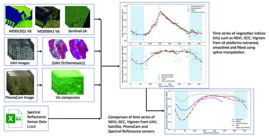
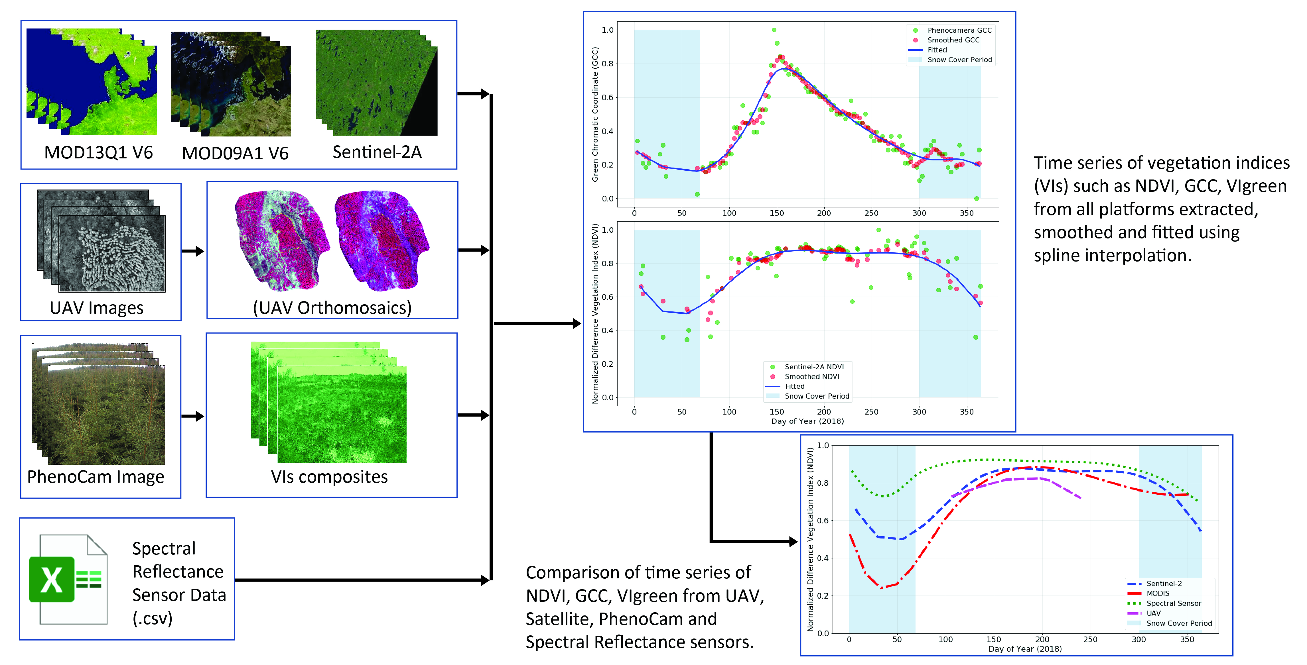
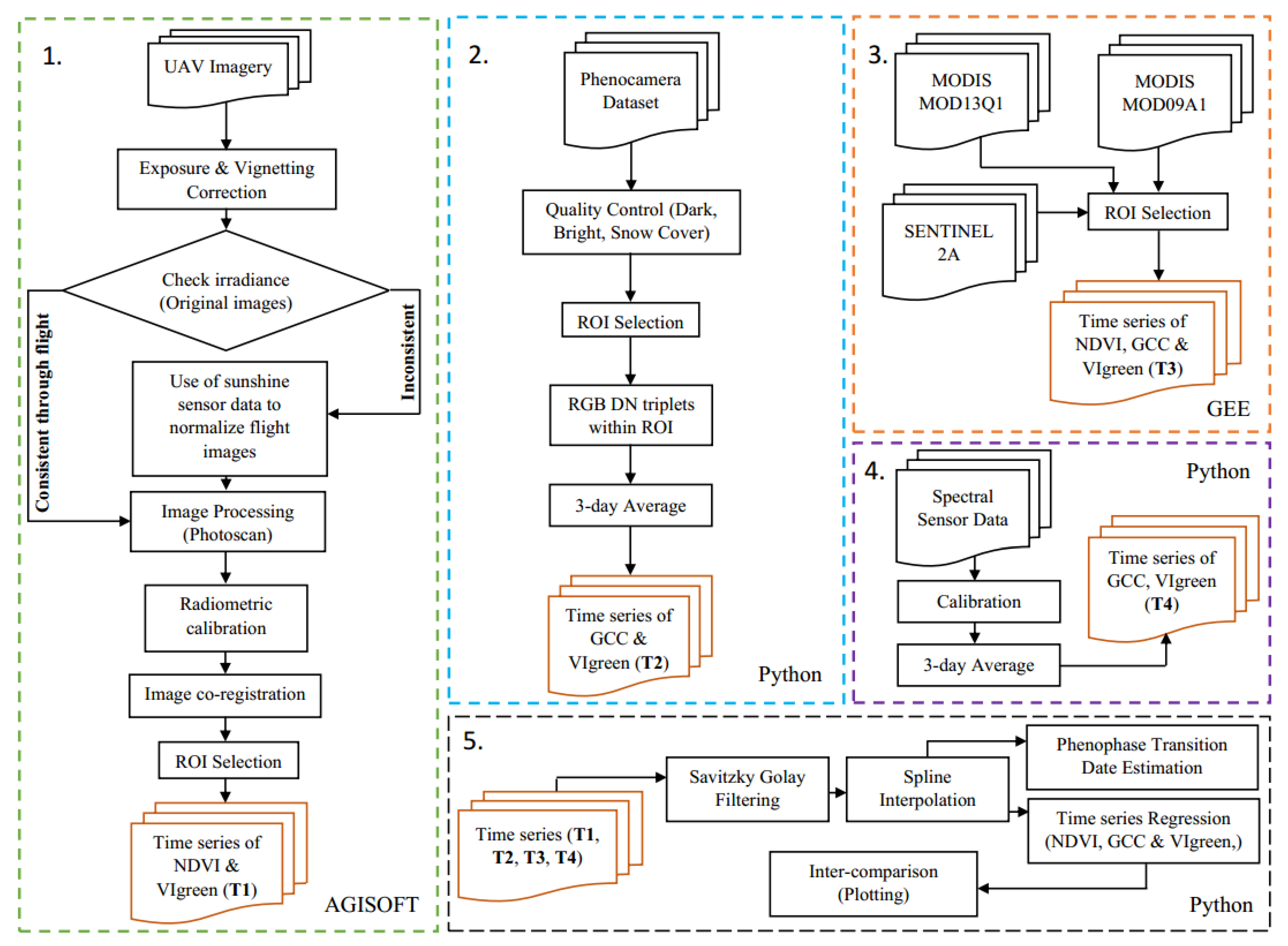
In recent years, the end-to-end (i.e., user to product) development strategy of different near-surface remote sensing systems have simplified the data processing and VI calculation, hence offering end-users the best decisions of use. With a view to further exploring the performance of such sensors building upon previous research, this study aims to test the ability of each sensor for tracking all-year phenology patterns. The main objective of this research is to explore the different aspects of vegetation phenology based on observations of different near-surface and satellite sensors, and to experimentally test and compare how consistent the time series of VIs obtained from different sensors are. Furthermore, the comparison provides insights on the reliability of VIs calculated from each sensor, the capability of each sensor to monitor seasonal dynamics, similarities and limitations of each index and platforms and the causes of these. This research considered three near-surface sensors (UAV, PhenoCam and SRS) and two satellite sensors of different spatial resolution (MODIS and Sentinel-2).

2. Study Area

The study area (Figure 1) consists of around 900 ha of mixed coniferous forest of spruce, pine and deciduous trees at Asa Forest Research Station [39], which is part of the Swedish Infrastructure for Ecosystem Science (SITES) project. Asa is located 37 km north of Växjö (57°8′59″ N, 14°44′17″ E). The study area is characterized by hemiboreal climate with mean annual temperature of 6.4 °C. The terrain within the area has flat topography in the south-eastern and western part, while the north-western part has a relatively elevated area with an altitude of approximately 212–248 metres above mean sea level (Figure 1b). The forest stand at Asa was planted in 2006 and it has been fertilized every second year since 2016. The variation in tree growth (height, diameter), field vegetation dynamics and phenology studies are routinely carried out. The area surveyed by the spectral sensors (SRS, UAV and PhenoCam) is a coniferous forest composed by Norway spruce (Picea abies). The forest is part of the Asa High Yield Experimental Forest, which addresses questions regarding intensive forest management at landscape level, such as fertilization and water quality, tree species introduction and their influence on flora and fauna.

3. Data

3.1. PhenoCam

The study used data from one facing south, mounted on a tower, at a height of 7.25 m above ground level, pointing 45° down from the horizontal, which captures digital imagery of the foreground canopy inside a field-of-view (FOV) of 60°. The PhenoCam images were acquired by a Mobotix 5 MP RGB camera. The camera captures a coloured three-layer R, G and B images at hourly temporal resolution from 5 a.m. to 8 p.m. all year long. The images for the year 2018 were downloaded from the SITES project server [40]. For this study, we used only images between 10 a.m. and 2 p.m., to avoid low solar elevation.

3.2. Unmanned Aerial Vehicles (UAVs)

For this study, we used data captured by a Parrot Sequoia multispectral camera (Parrot Drone SAS, Paris, France) [41] mounted on a Solo 3DR UAV (3DR Robotics, California, USA) [42]. The UAV system (UAS) payload capability comprises a Global Navigation Satellite System (GNSS), an Inertial Motion System (IMU), an accelerometer, a compass, and the camera system. The sensor onboard UAV captured data from an area covering around 10 hectares. Figure 2 illustrates the UAV platform and Parrot Sequoia sensor used in the study.

The Parrot Sequoia camera is designed to acquire images in four spectral bands: green (G), red (R), Red Edge (RE) and near-infrared (NIR), with wavelengths specified in

Table 1. Spectral band information for the near-surface multispectral sensors (Parrot Sequoia onboard UAV and Spectral Reflectance Sensors), satellite spectrometers (MODIS and Sentinel-2) and RGB PhenoCam. Only the spectral bands which were used in the research are mentioned here.

	Spectral Bands (nm)
Sensor	Blue (B)	Green (G)	Red (R)	Near-infrared (NIR)
Parrot Sequoia	-	550 ± 40	660 ± 40	790 ± 40
MODIS	469 ± 20	555 ± 20	645 ± 50	858.5 ± 35
Sentinel-2	490 ± 65	560 ± 35	665 ± 30	842 ± 115
SRS-NDVI	-	-	650 ± 10	810 ± 10
SRS-PRI	-	531 ± 10, 570 ± 10	-	-
PhenoCam	400–500	500–600	600–700	-

Note: B, G, R and NIR are defined by bands: B2, B3, B4, B8 for Sentinel-2, while B3, B4, B1, B2 for MODIS. Spectral bands in case of PhenoCam is presented as ranges, while it is central wavelength and bandwidth for the other sensors.

. The multispectral camera was installed under the drone facing the forest canopy. The images were captured by 1.2 MP monochrome sensors at a bit depth of 16 bit in raw format and later saved as .tif files.

The UAV flight frequency for the study period was roughly one flight per month from April to August 2018. The flights were not conducted in a fixed interval of time mainly because of weather conditions. The UAV was programmed to fly at a height of 80 m above ground level with frontal and side overlap of 80%. Most of the flights were conducted at midday (between 9 a.m. and 4 p.m.) on either clear days or evenly overcast days. The UAV was pre-programmed to follow the waypoints that would cover up the study area in two flights of approximately 10 min each. The camera and image settings were kept identical for all flights, in auto mode (i.e., camera chooses shutter speed and ISO value, while it has a fixed aperture) for exposure compensation. During the missions, the incoming radiation was measured and recorded by the sunshine sensor mounted on top of the UAV. The purpose of using the sunshine sensor was to normalize the images for variations in incoming sunlight, and for calculation of reflectance.

Three Spectralon reflectance panels (Labsphere, North Sutton, NH, USA), often defined as ground calibration targets (GCTs), and eight ground control points (GCPs) were placed within the UAV survey’s coverage on all flight dates for the purpose of radiometric calibration and georeferencing, respectively. Detailed information on all of the UAV flights carried out during the study period is listed in

Table 2. Information on the UAV missions conducted during 2018 with corresponding number of images and weather conditions. Note ‘*’represents one flight for which images were not processed due to large variation in irradiance data during the flight.

No.	Flight Date	Flying Height (m)	Flight Time (Local Time)	No. of Images	Weather Conditions	Status
1	2018-04-16	80	12:20	2233	Cloudy	✓
2	2018-04-25	80	10:30	2170	Cloudy	✓
3	2018-05-04	80	14:15	2088	Partly cloudy	✓
4	2018-05-15	80	13:00	2756	Cloudy	✓
5	2018-06-12	80	12:35	2716	Cloudy	✓
6	2018-06-26	80	09:45	2734	Mixed (Sunny, cloudy)	*
7	2018-07-09	80	12:15	2772	Sunny	✓
8	2018-07-26	80	12:00	2736	Sunny	✓
9	2018-08-28	80	13:45	2780	Cloudy	✓

Data Source: data.fieldsites.se. All datasets have unique PID which are mentioned in Appendix A (Table A1).

.

3.3. Spectral Reflectance Sensors (SRS)

The SRS used for this study were two two-band Decagon radiometers designed to measure the incident and reflected radiation in green, red and near-infrared (NIR) wavelengths suitable for the computation of NDVI (SRS-NDVI, hereafter) and photochemical reflectance index (PRI) (SRS-PRI, hereafter). The SRS-NDVI system is comprised of a pair of sensors: the SRS hemispherical, and the SRS field-stop lens sensor. The first type has a hemispherical 180° FOV, and is installed looking up to measure incident radiation, whereas the second type has a FOV confined to 36° for measuring downward reflected radiation from the forest canopy.

The SRS are mounted on the same tower as the PhenoCam, at the same height of 7.25 m, above the canopy of the spruce forest. Upward and downward-looking sensors measure the incident and reflected canopy radiance, respectively, simultaneously every 10 s, at a wavelength band specified in Table 1, with data aggregated to 10-min intervals. The data have been obtained from the SITES data portal [43].

3.4. Earth Observation Satellite Data

A time series of MODIS NDVI global product MOD13Q1 V6 [44] was obtained over the study area for the year 2018. This product, available as an image collection in Google Earth Engine (GEE) [45], provided NDVI values on a per-pixel basis generated every 16 days at 250 m spatial resolution. In addition, for greenness change estimates from visible bands, the MOD09A1 V6 [46] product, also available in GEE [47], was used, which provides surface spectral reflectance of MODIS Terra bands 1–7 at 500 m resolution corrected for atmospheric conditions.

In addition, from the GEE archive, a time series of surface reflectance in red and near-Infrared bands were derived from Sentinel-2A (bands 4 and 8, respectively) [48], which were used to compute NDVI at 10 metres spatial resolution. For the MODIS product, VI values of a single pixel were extracted. The comparison of UAV and Sentinel-2A vegetation indices with MODIS were based on a spatial average of all pixels that falls within ground projected footprint of the MODIS pixel. For the case of Sentinel-2A comparison against SRS, it was equivalent to the spatial average of all pixels within the ground projected footprint of the SRS.

4. Methodology

Our workflow comprised four processing steps: (1) data collection, (2) data extraction/processing, (3) data smoothing, and (4) phenophase transition dates estimation. Finally, an inter-comparison of smoothed time series information from all platforms and evaluation of correlations between data types was carried out. The details are described after the methodology chart (Figure 3). All the stated python script for PhenoCam image processing and Google Earth Engine (GEE) codes for extracting reflectance and different VIs that were written as a part of this research are available in https://github.com/shangharsha2929/ASA.git (accessed on 7 March 2021).

4.1. Phenocam Image Processing

First, the PhenoCam images that appeared disoriented, very bright (i.e., affected by solar glare), foggy, blurred, or had stripes covering more than 90% area of the image were removed manually before processing the images. In addition, snow-covered images were also filtered out so that the VI values from those could be computed separately. All the images that passed these quality control filters were used to compute the time series of vegetation indices. As per the experiment conducted by [31], the images captured at dawn and dusk experience low levels of diffuse sunlight, and are inclined to have lower VI values, compared to those recorded at middle day. With this finding in mind, of all valid images, only images between 10 a.m. to 3 p.m. (solar time) were used in the analysis.

Secondly, a rectangular region of interest (ROI) was defined within each digital image representing a sample of the spruce forest, from which the time series of RGB Digital Number (DN) triplets were extracted. The ROI was constant for all images. An effort was made to confirm that the time series was not affected by camera movements, which would result in a different ROI. When camera movements were detected, these images were processed separately by using a revised ROI that fit the same area of spruce forest. Figure 4 depicts the ROI selected for the study.

The DN values distributed across all the pixels in the corresponding ROI were extracted with a python code (involves use of OpenCV and NumPy module) that extracted the mean DN values of RGB bands across the defined ROIs. Then, the extracted mean DN values were fed into Equations (1) and (2) to compute GCC and VIgreen, respectively.

$$GCC=\frac{D{N}_G}{\left(D{N}_R+D{N}_G+D{N}_B\right)},$$

(1)

$$VIgreen=\frac{\left(D{N}_G-D{N}_R\right)}{\left(D{N}_G+D{N}_R\right)},$$

(2)

where $D{N}_R$ = mean red DN, $D{N}_G$ = mean green DN and $D{N}_B$ = mean blue DN for the chosen ROI.

With the calculation of these indices, the impact of variations in scene illumination is minimized [2,31,34,49].

For most of the applications, a very high temporal resolution (e.g., sub-hourly resolution, like in our study) seems unnecessary. This is because, in general, the vegetation colour over such short period of time remains relatively constant. With this consideration in mind, we preferred to calculate 3-day averages [49] of all the valid images for the vegetation indices mentioned above.

4.2. UAV Image Processing

First, the sunshine sensor data from all UAV flights were retrieved from the images’ metadata and then plotted, to check the incoming light conditions for each single band (G, R, RE and NIR).

The UAV flights that presented irregular and complex light variability during the flight (Figure 5c) were discarded. The data that presented constant light, under sunny (Figure 5a) or overcast sky (Figure 5b), were further processed. The information regarding the flights that were accepted or rejected for further processing is listed in Table 2. Based on this information, UAV data were characterized in three ways: (1) consistent sunny incoming light, (2) consistent cloudy incoming light, with slight variation, and (3) complex incoming light recorded during the mission. The three different cases are depicted as a, b and c in Figure 5, respectively.

After categorizing the flights, the individual images of each flight data were subjected to exposure calibration, vignetting correction and irradiance normalization. These corrections were carried out in accordance with a recently developed methodology [50]. To adjust for different exposure settings of images, exposure calibration according to Equation (3) provided by Parrot Sequoia was performed.

$$L_p=f^2\frac{DN-B}{A\epsilon \gamma +C},$$

(3)

where $L_p$ is pseudo-radiance defined in an arbitrary unit common to all Sequoia cameras, the aperture f-number (f = 2.2 for Sequoia), the digital number of a pixel (DN), exposure time (ε), ISO value (γ) and A, B, C are calibration coefficients provided in the image metadata.

Vignetting is defined as a radial fall-off in pixel values that results in darker areas near the edges of images [17]. The method for minimizing the vignetting effect was based on the use of vignetting polynomial [51] derived from the EXIF/XMP metadata of the Sequoia images. The vignetting polynomial estimation as explained in [50] was based on finding a correction factor for each pixel from a large number of images captured over a Lambertian surface and these pixel-wise correction factors fitted by a polynomial.

Only flight data showing the consistent irradiance throughout the mission (Figure 6a) was processed for the exposure and vignetting correction. Similarly, the flight data that showed variation in irradiance data that could be handled by normalizing for incoming light condition from sunshine sensor data (Figure 6b) were normalized using a polynomial trend of degree ‘n’ or spline trend, based on the nature of the data [50]. The best fit polynomial or splines were selected based on visual inspection by manually fitting to the data. The degree of polynomial was chosen in such a way that it fit the irradiance data with coherence at the start and end of each flight. This is because the GCT images were captured only at the beginning and end of the mission, which were later used for radiometric calibration of the derived orthophotos. The detailed process regarding the exposure, vignetting and irradiance normalization are explained in [50].

A significant number of pixels reached the top of the spectral range (saturation) in the images of each flight, mostly in the G band and least in the NIR band. This problem is also mentioned by [50,52]. The saturated pixels were generally over bright surfaces (i.e., rocks or gravel soil) on the ground. As these saturated pixels influence the orthophotos, they were masked out [50].

All the flight images that had undergone the process of these corrections were thereafter imported into Photoscan 1.4.2 (Agisoft, St. Petersburg, Russia), a photogrammetry software package for image orthorectification (

Table 3. Main parameters used in Agisoft Photoscan 1.4.2. under different steps of image processing to create orthophotos from each set of flight data.

Steps	Parameters
Align Photos	Accuracy: High; Pair selection: Ground control; Point limit: 40,000; Constrain features by mask: No.
Build Dense Point Cloud	Quality: High; Depth filtering: Aggressive; Reuse depth maps: No.
Build DEM	Source data: Dense point cloud; Interpolation: Enabled.
Build Orthophoto	Surface: DEM data; Blending mode: Mosaic(default).

).

Five out of eight GCPs were used to produce a georeferenced orthomosaic with a nominal spatial resolution of 0.07 m. The other three GCP markers were used as check points, which resulted in a root mean squared error (RMSE) of 0.02 m. Only one orthomosaic (dated 2018-07-17) was georeferenced in Photoscan and this was then used as a reference to co-register the rest of the orthomosaics (eight in total) by using same GCP markers.

Finally, the orthomosaics were subjected to radiometric calibration using the empirical line method suggested by [53]. The method relies on mean pixel values of three Spectralon reflectance panels (GCTs) present in the images and their standard reflectance values. The standard reflectance values were black (5%), dark grey (20%) and light grey (50%). The standard reflectance value of these panels, together with the mean DN of the same panel extracted from a set of images, were used to convert the orthomosaics into reflectance, by establishing a linear relationship between the measurements.

The radiometrically corrected orthomosaics were then used to compute NDVI maps, for all flights. NDVI, with a dynamic range of −1 to +1 [16] was calculated according to Equation (4):

$$NDVI=\frac{{\rho }_{NIR}-{\rho }_{RED}}{{\rho }_{NIR}+{\rho }_{RED}},$$

(4)

where ${\rho }_{NIR}$ = near-infrared reflectance, and ${\rho }_{RED}$ = visual red reflectance. The values around 0 represent bare soil and values of 1 refers to vigorous vegetation. The footprint of the SRS was projected on top of the NDVI maps to extract the values of NDVI of the UAV flights, for comparison with other sensors.

Figure 6 shows the spatial variation of NDVI over the study area. Low-lying areas in the NE part of the region represent wet bare lands, which are characterized by intermediate NDVI values. The patterns of trees are clearly visible and are characterized by high NDVI values. It shows low NDVI values within the forest representing bare soil. Higher NDVI values in open areas refer to the presence of low-lying vegetation such as bushes and ferns. Lower values are in the SW, representing rock outcrop, and along a barren stream on the eastern side.

4.3. Satellite Data Processing

An automated approach was developed to extract the NDVI values for the study area, from the global MODIS NDVI product MOD13Q1 on the GEE platform (Figure 7). The NDVI from Sentinel-2A was not directly available in GEE; therefore, the corresponding band values required to compute NDVI (R and NIR reflectance from bands 4 and 8, respectively) were used. In addition, all three RGB band values of MODIS (MOD09A1 product) and Sentinel-2A, for the common area similar to SRS were extracted and later used to compute GCC and VIgreen by using GEE. These GCC and VIgreen values were downloaded as .csv files, which were further used on to compute the seasonality events. The cloudy pixels, in the case of Sentinel-2 images, were masked out using available cloud mask band ‘QA60’ within GEE platform.

4.4. Spectral Reflectance Sensor Data Processing

The irradiance data from SRS were calibrated using calibration factors of 0.250 (R) and 0.260 (NIR) in the case of SRS-NDVI sensor, and 0.259 (570 nm) for the SRS-PRI sensor following methodology in [54]. A subset of measurements was extracted from the full time series, which covered exactly between the same hours as the period used for the PhenoCam (9 a.m. to 3 p.m.). The calculation of SRS-NDVI was done on reflectance, calculated as a ratio from incoming and reflected radiation, by dividing the downward-looking by the upward-looking sensor data. The data was averaged in similar time aggregates as the PhenoCam, i.e., 3-day averaged NDVI values. In addition to the NDVI, VIgreen was computed in a similar fashion to the PhenoCam, combining the red band from the NDVI-SRS and one of the green bands at 570 nm from the SRS-PRI sensor. The footprint of the SRS was computed using the sensor characteristics (i.e., FOV: 36°, height: 7.25 m, off-nadir angle: 45°) and the tower coordinates. The same footprint was used across all sensors to extract time series of VI values for effective comparison.

4.5. Curve Fitting to Time Series Data

The original time series data obtained from different platforms (UAV, PhenoCam, satellite and SRS) were processed with the Savitzky-Golay filter [4,55,56] to remove residual irregular changes of VI values in the annual cycle. This process was performed using a first-degree polynomial with a window size of 3 (in the case of UAV-derived NDVI time series) and 5 (in case of the PhenoCam, satellite and SRS-based VI time series). Of all the different curve fitting methods explained in [57], univariate spline interpolation was used to fit the time series data [49] from all studied platforms, as it led to the best fit.

The phenology transition dates estimation was based on the fitted spline curves, which were calculated based on the rate of change in curvature [4,57,58]. The rate of change in curvature (k) is defined in Equation (4) as:

$$k=\frac{f^{″}\left(t\right)}{{\left(1+{\left(f^{\prime }\left(t\right)\right)}^2\right)}^{3/2}}$$

(5)

where $f^{\prime }\left(t\right)$ and, $f″\left(t\right)$ are the first and second order derivatives, respectively of the spline fit.

The phenological transition dates for the green-up phase were defined as the times at which the rate of change in curvature exhibits local minima or maxima. These extremes were used to extract start, end, and middle of the spring season (SOS, MOS, and EOS, respectively), in a similar fashion to [11,57]. The local extreme values approximately correspond to 10, 50 and 90% of amplitude in the spring green-up phase of vegetation growth [57].

4.6. Sensor Inter-Comparison

The time series data and phenophase transition dates from the studied platforms were analysed at three levels: (1) graphical comparison of VI time series from the different sensors, (2) regression analyses between the time series information, and (3) estimation of the biases in number of days of the transition dates, compared to visual inspection of PhenoCam photos. All three steps were applied to curve-fitted time series data. For regression analysis, using root mean square deviation (RMSD) and Pearson’s correlation coefficient were used.

NDVI was originally planned as the common VI to compare across the different studies sensors, as it has been widely used in many remote sensing studies. However, since NDVI cannot be calculated from PhenoCam data, as it does not have NIR band, GCC was used instead to compare PhenoCam VIs against satellite derived indices. In the same manner, GCC cannot be calculated for SRS, as a blue band is not available. Therefore, VIgreen was used as a common VI to compare data from all platforms, as red and green bands were available for all studied sensors. Since the different VI ranges are expressed in different units and scale, they were normalized by using the min-max normalization [59], as a means to match all the values to be in the range of 0–1, for graphical comparison of VIs across different sensors, except for the comparison of NDVI from different platforms (Section 5.2.). For NDVI, we used the original values (between −1 and 1) and not the normalized ones. For the regression analysis, also original VI values were used.

The calculation of RMSD and correlation coefficients included fitted time series data during the green-up, growing and senescence phases (DOY 70−300) across all systems. This was done to avoid the snow season and focus on the vegetation growing season.

For estimating bias in transition dates, SOS was defined as the DOY when the green sprouts started to be visible on the PhenoCam images, while EOS was defined as the day when sprouts were fully developed and could no longer be differentiated from the rest of the branches. In SOS, the sprouts are easily recognizable as they are bright green, while EOS was defined when the sprouts get a darker colour, similar to the rest of the tree (Figure 8).

Since the studied forest was evergreen and the changes in vegetation could not be differentiated with a human eye, it was not possible to define the dates for other seasonality events (i.e., end of the growing season and beginning of the senescence phase). The agreement between the phenophase dates from all sensors were compared against visual inspection data in the PhenoCam imagery, and the phenophase dates calculated statistically, expressed as bias in number of days.

5. Results

5.1. Spline Fit Time Series of VIs Derived from Different Sensors

The time series of different VIs fitted with the spline interpolation technique are depicted in Figure 9. The snow period at the beginning and end of the year (blue rectangles in the figure based on PhenoCam images) influenced the VI values in almost all of the sensor types. The middle of the season peak is much more pronounced in GCC (Figure 9a–c) and VIgreen (Figure 9d–f), with well-defined seasonal start, peak, and end, and similar in shape, in general, across different sensors. The exception is VIgreen for SRS (Figure 9g), which does not show a clear peak in the middle of the growing season, nor pronounced slopes at the beginning and end of it. The fitted curve for Sentinel-2 NDVI (Figure 9i) is flatter compared to VIgreen and GCC, with less pronounced slopes at the beginning and end of the growing season. Nevertheless, as per VIgreen and GCC, the shape of NDVI is similar across sensors. UAV-based VI values show the spline fit only during the middle part of growing season as the flights were conducted only during that period (Figure 9k).

In the following sections, we plot each of the VIs for the different sensors, for a more detailed comparison.

5.2. Comparison of NDVI Derived from Different Sensors

Figure 10 shows a plot of spline fitted curves from UAV_NDVI, SRS_NDVI, MODIS_NDVI and Sentinel-2_NDVI. The plot indicates that the four datasets follow the similar trend in general throughout the growing season. However, they differ at the start and end of the time series, as they show significant different slopes and offset. The discrepancy between the SRS_NDVI, Sentinel-2_NDVI and MODIS_NDVI is most pronounced at the beginning of the year until end of February, being the satellite_NDVI values lower than the SRS_NDVI values, and significantly lower for Sentinel-2_NDVI also at the end of the season, from October to December. These low NDVI values could be due to the snow cover, higher decline in satellite data as they are viewing more snow-covered ground than the SRS_NDVI, which also show reflectance leaves and branches. Additionally, there can be a different light scattering at the top of the atmosphere, observed by the satellites, than near the ground, as observed by the SRS_NDVI. After May, we observe a stabilization of NDVI values until the end of October (please note that, for the UAV_NDVI sensor, the time series ends in September). There is, however, certain offset between NDVI values across sensors, ranging from 0.8 (UAV_NDVI) to 0.9 (SRS_NDVI) at the peak of the season. As NDVI ranges from −1 to 1, this difference accounts for a 5% difference in reflectance between UAV_NDVI and SRS_NDVI. The green-up phase (March to May) is depicted very differently across sensors. In this time of the year, the differences cannot be attributed to snow. The slope for satellite data is significantly higher than for SRS_NDVI, and the offset rises to a 25% between MODIS_NDVI (0.4) and SRS_NDVI (0.9).

According to the Pearson’s regression analysis, the NDVI values from all sensors were positively correlated with each other (

Table 4. Pearson’s correlation coefficient (r) and RMSD in NDVI units computed between UAVNDVI, SRSNDVI, MODISNDVI and Sentinel-2NDVI. N is sample size (total number of time series data).

Sensor A vs. Sensor B	Pearson’s Correlation Coefficient (r)	RMSD	N
UAV—SRS	0.84 *	0.14	42
UAV—MODIS	0.75 *	0.08	18
UAV—Sentinel-2	0.77 *	0.06	44
MODIS—Sentinel-2	0.92 **	0.08	21
SRS—MODIS	0.81 **	0.09	28
SRS—Sentinel-2	0.79 **	0.07	61

** p < 0.001; * p < 0.05.

). The correlation between UAV_NDVI and MODIS_NDVI was the lowest (r = 0.75; RMSD = 0.08), while the highest correlation was found between MODIS_NDVI and Sentinel-2_NDVI (r = 0.92; RMSE = 0.08), indicating a better fit between the two satellite datasets.

5.3. Comparison of GCC from Different Sensor Types

The PhenoCam_GCC, MODIS_GCC and Sentinel-2_GCC followed quite similar seasonal pattern (Figure 11). The plot shows that the canopy GCC signal followed a similar green-up response, while the GCC trajectories separate a little after reaching the peak of the growing season (PhenoCam_GCC vs. satellite_GCC) and during the senescence phase (MODIS_GCC against the rest). Additionally, the peak of PhenoCam_GCC is separated by a vertical offset of around 0.2 units from the satellite_GCC (0.78–0.9). Moreover, the peak of the season is slightly different for PhenoCam_GCC (around June 1st) than for satellite_GCC (around 24 June).

The Pearson’s correlation coefficients computed between the GCC values from these sensors are presented in

Table 5. Pearson’s correlation coefficient (r) and RMSD between PhenoCam_GCC, MODIS_GCC and Sentinel-2_GCC. N is sample size.

Sensor A vs. Sensor B	Pearson’s Correlation Coefficient (r)	RMSD	N
PhenoCam—MODIS	0.93 **	0.11	42
PhenoCam—Sentinel-2	0.97 **	0.09	88
MODIS—Sentinel-2	0.93 **	0.10	43

** p < 0.001; * p < 0.05.

. PhenoCam_GCC was in good agreement with MODIS_GCC and Sentinel-2_GCC as reflected in high positive correlation coefficients (0.93 and 0.97, respectively) with approximately 10% deviation on an average.

5.4. Comparison of VIgreen from Different Sensor Types

Plots of VIgreen for all the sensor types are shown in Figure 12. The time series obtained from PhenoCam_VIgreen, UAV_VIgreen, MODIS_VIgreen, and Sentinel-2_VIgreen appeared to follow a similar seasonal pattern, compared to the one obtained from SRS_VIgreen, where the time series are flatter along the growing season. A detailed comparison shows that for PhenoCam_VIgreen the green-up phase starts later (DOY~ 125) and the slope is almost vertical. Another significant difference is observed in UAV_VIgreen, which peaks later than PhenoCam_VIgreen and satellite_VIgreen data, around DOY = 200 vs. DOY~150. Additionally, the VIgreen values differ in the senescence phase; the slope is more pronounced and starts earlier for PhenoCam_VIgreen; it is a gradual slope for MODIS_VIgreen, and also a steep slope and later slope for Sentinel-2_VIgreen and UAV_VIgreen.

The Pearson’s correlation coefficients computed for VIgreen from these sensors are presented in

Table 6. Pearson’s correlation coefficient (r) and RMSD for PhenoCam_VIgreen, MODIS_VIgreen, Sentinel-2_VIgreen, SRS_VIgreen, and UAV_VIgreen. N is sample size.

Sensor A vs. Sensor B	Pearson’s Correlation Coefficient (r)	RMSD	N
PhenoCam—MODIS	0.83 **	0.13	25
PhenoCam—Sentinel-2	0.79 **	0.22	23
PhenoCam—SRS	0.63 **	0.44	70
PhenoCam—UAV	0.85 *	0.58	8
MODIS—Sentinel-2	0.92 **	0.14	41
MODIS—SRS	0.64 **	0.35	37
MODIS—UAV	0.89 *	0.42	8
Sentinel-2—SRS	0.58 *	0.46	84
Sentinel-2—UAV	0.71 *	0.38	8
SRS—UAV	0.91 *	0.14	8

** p < 0.001; * p < 0.05.

. PhenoCam_VIgreen, MODIS_VIgreen and Sentinel-2_VIgreen were not so strongly correlated (r = 0.63, 0.64 and 0.58, respectively) with SRS_VIgreen, while the rest of sensor types are moderately correlated among each other (r > 0.7).

5.5. Evaluating Phenophase Transition Dates from All Platforms

Phenological transition dates derived from visual inspection were compared with those from spline fitted time VIs from the different platforms to detect the different phases of the growing season in the studied spruce forest. The bias (in number of days) between the reference start and end of season (based on visual inspection) compared to the phenophase transition dates calculated from VIs, for all the platforms except the SRS, are shown in

Table 7. Estimates of Start of Spring (SOS), Middle of Spring (MOS), and End of Spring (EOS), in day of year, computed using spline fitted time series of GCC, VIgreen, NDVI from all the platforms studied, and bias in number of days, with respect to visual inspection. Note ‘*’ represents no UAV flight data, thereby no bias.

		Seasonality Parameters (DOY)			Visual Inspection (DOY)		Bias (days)
Vegetation Indices	Sensor	SOS	MOS	EOS	SOS	EOS	∆SOS	∆EOS
GCC	PhenoCam	93	132	147	90	150	3	−3
	MODIS	96	123	153			6	3
	Sentinel-2	93	129	153			3	3
VIgreen	PhenoCam	99	132	147			9	−3
	MODIS	96	123	147			6	−3
	Sentinel-2	96	123	147			6	−3
	UAV	*	130	154			*	4
NDVI	MODIS	98	129	158			8	8
	Sentinel-2	80	129	150			−10	0
	UAV	*	124	154			*	4

and Figure 9. SRS-based phenophase dates are not mentioned in the table and are not considered in the comparison with phenophase from other platforms. Irregular patterns of SRS-based VIs did not allow us to extract meaningful phenophase dates from the spline fitted curves, due to the flat nature of the SRS-VI profiles and the method employed for phenophase extraction (change in curvature).

According to the visual inspection of PhenoCam images, the Start of the Spring (SOS) happened in DOY: 90 (31 March) and ended in DOY: 150 (30 May). Seasonality parameters, mainly the SOS, MOS, and EOS extracted from all the platforms using the spline fitted time series of GCC, VIgreen and NDVI were observed to be consistently similar, except for the VIgreen from Sentinel-2, which showed very early SOS when compared to visual inspection data. Visually assessed dates (SOS and EOS) compared against dates estimated from other sensors showed a bias ranging from 3–10 days. The negative bias refers to earlier SOS and EOS. The maximum bias in SOS and EOS was observed in seasonality extracted from MODIS and Sentinel derived NDVI values, which accounted for 8 days in case of MODIS and 10 days in case of Sentinel-2. The minimum bias across all sensor types were the ones extracted from GCC with bias ranging between 3 and 6 days, while in case of VIgreen, the biases in SOS and EOS ranged between 3 and 9 days. No UAV flights were conducted as early as the SOS; hence, it was not possible to compute the bias.

6. Discussion

Using remote sensors to study vegetation phenology at different scales opens up the opportunity to gather information on different aspects of the life cycle of plants to better understand the interaction between climate change and the biosphere. While different near-surface and satellite sensors are available for vegetation phenology monitoring, few studies provide sensor overview and inter-comparisons [1,4,24,25]. In this research, an effort has been made to compare the performance of different remote sensors to characterize the phenology of a forest. Using combined methods of UAV photogrammetry, phenocamera data analysis, and multispectral sensor data analysis (SRS and satellite), we explored the difference between phenological time series obtained from these platforms, by means of spectral vegetation indices such as NDVI, VIgreen and GCC.

In this study, we observed the complementarity of the data from the studied remote sensors for characterizing vegetation phenology in an evergreen coniferous forest. PhenoCams and SRS offer the flexibility of defining regions of interest within very fine spatio-temporal resolution images (hourly, tree level), and thus allows researchers to model the phenology dynamics of the observed ecosystem, for either individual or a group of species within the landscape. On the other hand, satellite observations cover large regions for global observations [5], at coarser spatial (decametres to kilometres) and temporal resolutions (days to months). UAVs have the benefit of a fine pixel size (nominally, a few centimetres) and can be operated frequently and avoid atmospheric effects [4].

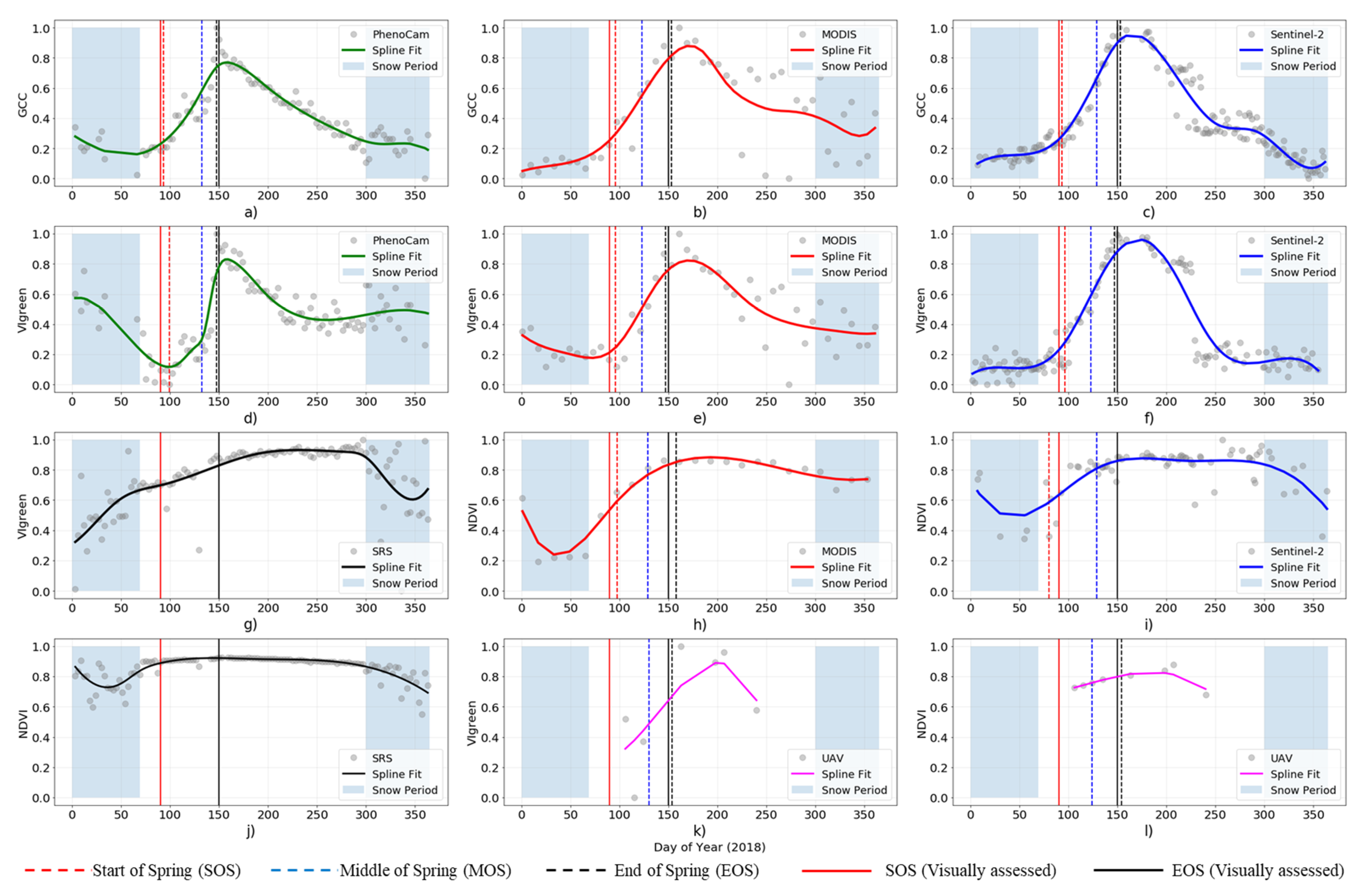
Our results show that there are similarities between VIs of the different studied sensors in terms of shape of the phenology curves as indicated by Pearson’ correlation and RMSD showing good agreement between the VIs across the studied sensors. However, there are significant differences in slopes and offsets when comparing the time series of different sensors, for a given VI. As expected, the time series of satellite data (i.e., MODIS and Sentinel-2) are closely correlated and follow a similar time series shape. On the other hand, depending on the VI (NDVI, VIgreen or GCC), we observed different behaviours among sensors. For instance, we noted that UAV_NDVI data show a similar pattern to MODIS_NDVI and Sentinel-2_NDVI during the summertime (April to August). Additionally, there is a good agreement between PhenoCam_GCC and satellite_GCC for the green-up season (April to May). Regarding VIgreen, there is a relatively good match in determining the peak of the growing season (DOY ~150) between PhenoCam_VIgreen, MODIS_VIgreen and Sentinel-2_VIgreen, while the green-up slope of UAV_VIgreen and satellite_VIgreen also follow similar patterns. However, these are the only agreements between sensors; apart from these, all sensors differ in slopes on the green-up and senescence, the maximum VI value at the peak of the season, and the phenology transition dates (i.e., beginning, end and length of the growing season). A remarkable difference was observed in the behaviour of SRS sensors; SRS_NDVI and SRS_VIgreen show significantly higher values than any other sensors, and the length of the growing season is notably longer than for the rest of sensors. Additionally, RMSD related to SRS versus other sensors were generally large.

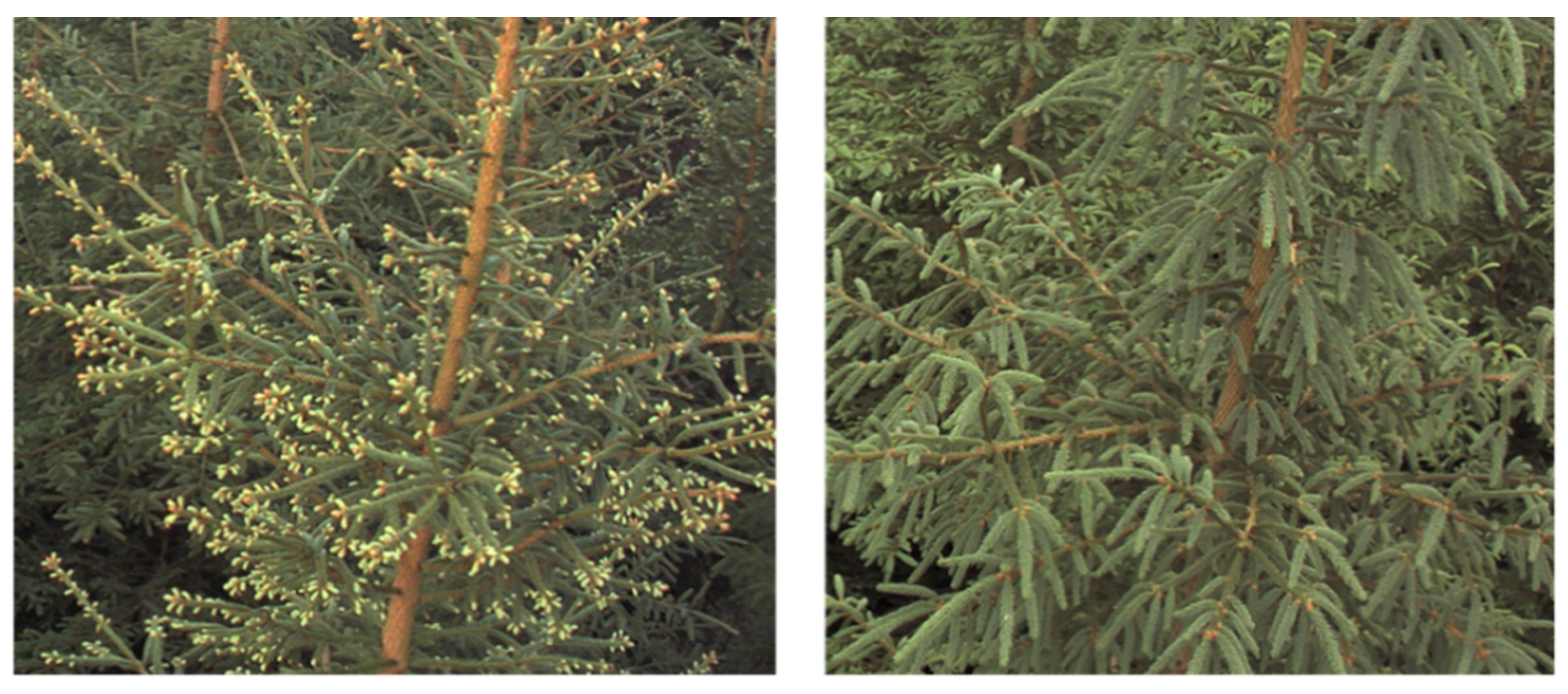
There are many reasons for the differences between the phenology time series, as described by the different VIs and sensor types. Primarily, it must be noted that the visual seasonal cycle is considerably weaker in evergreen forests than in deciduous forests, and the low annual production of green buds in boreal coniferous forests, in combination with the influence of snow, presents considerable difficulties for detecting the green-up and senescence phases using remote sensing [60]. Further reasons for the different performances of the sensors are the different spatial resolutions, different spectral band configurations, sensor calibrations, different viewing angles, or differences in data processing [14,24,25,32]. In addition, the spectral sensors have different spectral response functions, which could cause systematic deviations in the time series of spectral VIs derived from them [24,61]. One important factor that might cause differences in the VIs is the viewing angle. In particular, the PhenoCam points towards the horizon and views the canopies of the studied trees (i.e., profile view), while the other studied sensors view from the zenith, viewing the canopy of the trees vertically, including the understory vegetation, soil and snow, through the forest clearings. The varying viewing angles of the studied sensors influence the bidirectional reflectance distribution function (BRDF) [16]. This affects the spectral and VI values captured by each sensor type [4]. Moreover, the sun-sensor target viewing geometry is different between the near-ground sensors and the satellites. If we consider the geometry of a typical spruce forest as a collection of conical trees, the shadows projected by the trees influence the reflectance of the forest very differently [62,63], depending on the position of the observer (the sensor). If the sensor and the sun are aligned, the sunlight side of the forests is in the view field, whereas, if the observed target is between the sensor and the sun, the shaded side of the forest is in the view field [62].

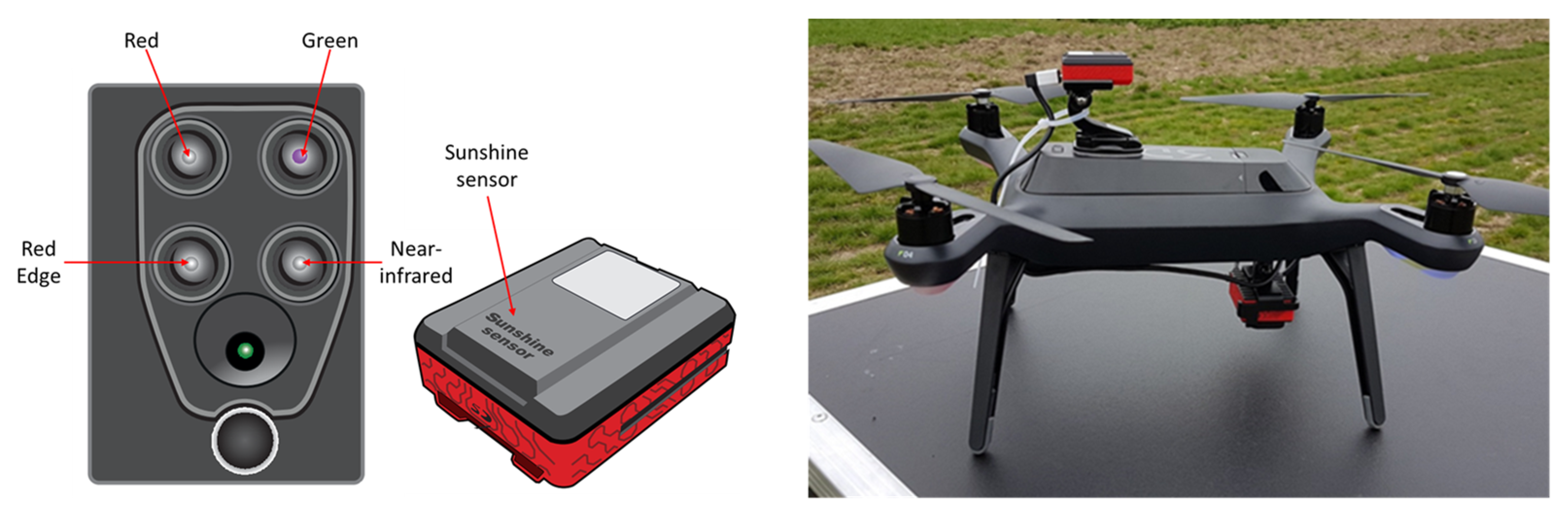
Another potential reason for the offset in VIs is the difference in the spectral range and bandwidth of each sensor. The highest difference in bandwidth range is observed in NIR and R (Sequoia: 40 nm; MODIS: 35 nm; Sentinel-2: 106 nm; SRS: 10 nm, for R and NIR). Additionally, the central wavelengths of the NIR bands are different (Table 2). Even though the central wavelengths of G and R bands were close in all sensors, there are significant differences in bandwidth (Sequoia: 40/40 nm, MODIS: 20/50 nm, Sentinel-2: 36/31 nm, and SRS: 10/10 nm for G and R, respectively). These differences affect the spectral VI values (NDVI, GCC and VIgreen) among sensors. Another reason for deviations in values of the VI time series could be the mixed reflectance characteristics caused by the different spatial resolution of the observed sensors. In addition, the specific days used for image compositing, observation time, and solar elevation angle might add differences in the measured spectral values [64]. In this study, there was a huge difference in spatial resolution of the sensors (MODIS: 250 m and 500 m, Sentinel-2: 10 m, UAV: ~8 cm, PhenoCam: ~17 m and SRS: ~8 m). With the increase or decrease of remote sensing image scale, the observed targets within a pixel at the ground surface, as seen by each of these sensors, are quite different. This will result in generation of mixed pixels [16] causing different signal intensities of mixed objects, when compared with the signal intensity of large-scale images. Despite the relative homogeneity of the analysed spruce forest, it is likely that data from the satellite sensors are affected by mixed targets, e.g., understory vegetation and soil. In addition, even though we selected the same observation time for UAV, SRS and PhenoCam for inter-comparison, there was a different acquisition time for the satellite sensors.

Despite the different performance of the selected VIs and studied platforms, we can conclude that different sensors address different aspects of the vegetation. These platforms are complementary when characterising phenology and they should be used for different purposes. As observed in our study, we found strong correlation and similar curve fitting between UAV_NDVI and satellite_NDVI. Therefore, UAV can be a solid tool for upscaling from near-ground observations to satellite data. Despite the differences in pixel size, Parrot Sequoia has a similar band configuration as MODIS and Sentinel-2 [41]. That is not the case for UAV_VIgreen versus MODIS_VIgreen and Sentinel-2_VIgreen, where the time series offset and slopes are very different. Our results coincide with the findings of [59], where VIgreen index from multiple cameras had the lowest correlation to MODIS in comparison to the GCC. Despite VIgreen being a normalized index like NDVI, the NIR band seem to play an important role in differentiating vegetation productivity [65,66]. We also observed a good agreement between PhenoCam_GCC and the satellites_GCC, especially in the green-up phase, as was also observed by [57,67], despite GCC not using the NIR band, and both sensor types having different viewing angles and pixel sizes [14]. This finding validates MODIS and Sentinel-2 as useful sensors for characterizing vegetation phenology at the landscape scale. In summary, the results suggest that VIgreen is not a good proxy for phenology, while NDVI and GCC are, as was previously observed by [2,4,13].

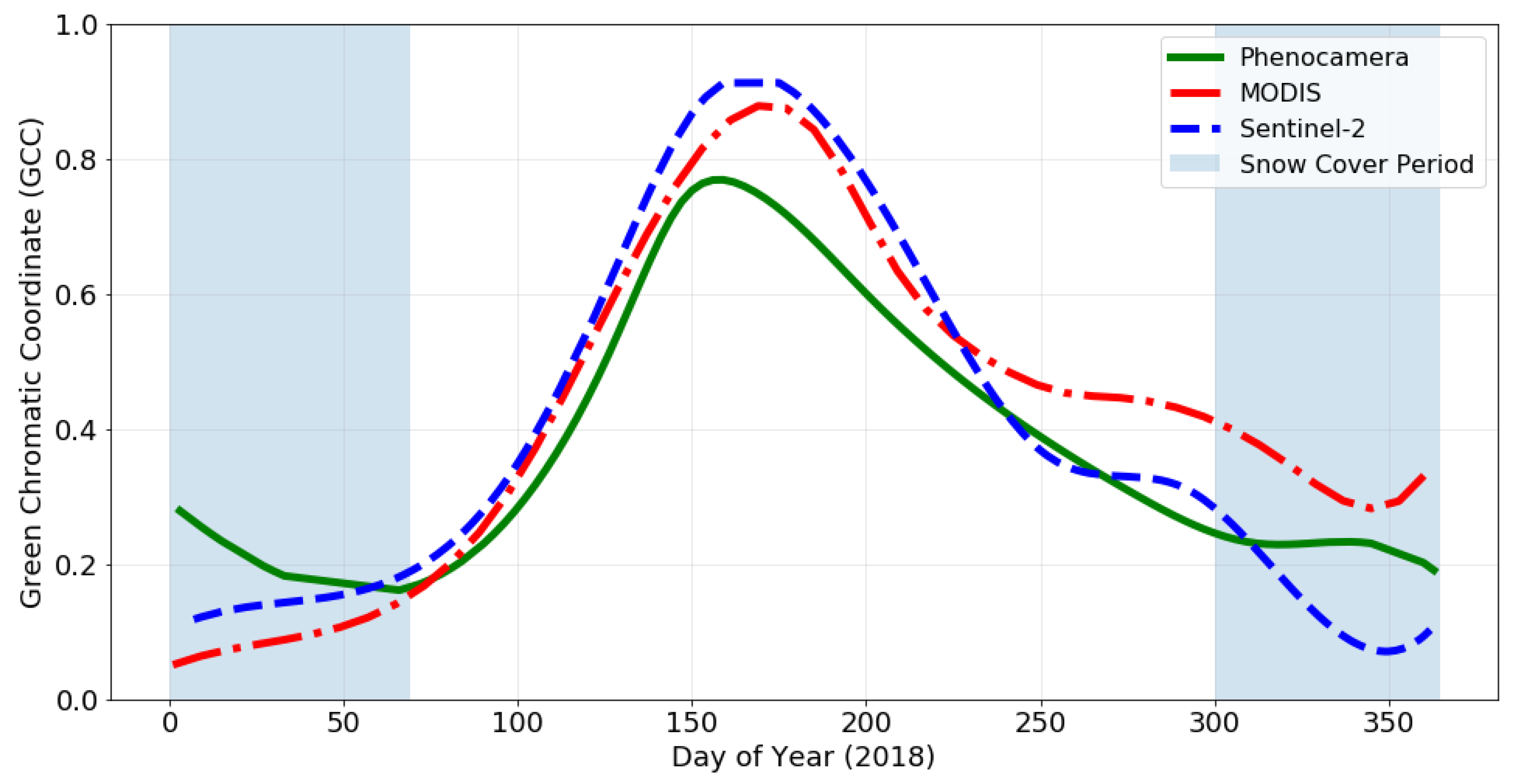
We observed strongly significant different time series pattern between NDVI and GCC (Figure 9). NDVI saturates at a high value throughout the growing season, with a short green-up and senescence phases. Additionally, for SRS_NDVI there is not a significant increase in NDVI between the green and the non-green seasons. On the contrary, GCC presents a sharper peak in the middle of the growing season, with steep slopes for the senescence phase, and especially for the green-up phase. Therefore, we hypothesize that NDVI, through its sensitivity to red light absorption, is more sensitive to the overall albedo change going from a snowy landscape to the fully developed green canopy. The sensitivity of NDVI is well documented [60,68,69]. On the other hand, the GCC normalizes for albedo and thereby amplifies the green signal of the canopy that relates more directly to the phenology phases. These VIs relate to different aspects of the changing landscape during spring. To note is that both VIs work well at both near-surface and landscape scales, as shown by the agreement between UAV_NDVI vs. satellite_NDVI and PhenoCam_GCC vs. satellite_GCC. Therefore, PhenoCams and UAVs have important and complementary roles for satellite data validation and upscaling [26,30,57,59,70].

An important observation of this study is the differences in offset between platforms. As mentioned, the shapes of the time series and correlations among VIs across sensors was strong, especially in summer time. However, we found significant differences in the slopes of the green-up and senescence phases, as well as significant offset in VI values, across sensor types. This suggests that these remote sensors can be interchangeable for qualitative characterization of vegetation phenology, especially of the growing season, but cannot be used indistinctively for quantitative studies or accurate determination of phenology phases [4,59,70]. Another result that supports this is that the statistical calculation of the phenology transition dates (SOS, MOS and EOS) using fitted time series curves from VIs shows certain biases with the real dates, captured in the PhenoCam images by visual inspection. The bias in estimating SOS and EOS was around three days for GCC, while it was up to 8–10 days for NDVI. For VIgreen, the bias ranged between 3 and 8 days. This supports the conclusion that NDVI and VIgreen may be less appropriate estimators of phenology phases than GCC [4,14,59].

A second conclusion of our study is that there is a large uncertainty and differences in VI performance among sensors during the winter season, when there is snow on the ground and trees. The presence of snow beneath the forest canopy is assumed to remain longer compared to the canopy mostly during the spring and can be detected differently across near-surface and satellite sensors [71]. This eventually affects SOS events derived from time series obtained from different platforms [72]. While the VI time series are somehow comparable when there is only vegetation present, the behaviour of the VIs is quite random from sensor to sensor in the presence of snow. Complex light scattering and viewing geometry, as well as the likelihood of snow on up-looking sensors, affect the different VI signals observed for snow [16,73,74].

7. Conclusions

In the present paper, near-surface and satellite remote sensors at different scales were inter-compared for the purpose of vegetation phenology characterization. We defined phenology time series from multispectral ground sensors (SRS), PhenoCam, UAV, Sentinel-2 and MODIS data, depicted by three different spectral vegetation indices (VIs), i.e., NDVI, GCC and VIgreen. These platforms differ significantly in spatial and temporal resolutions, viewing angles and observation scales. The aim of this study was therefore to explore differences in the time series phenology curves from sensor to sensor and for different Vis, and their performances in determining the transition dates in phenology along the year.

Based on the results, we conclude that the studied remote sensing platforms (SRS, UAV, PhenoCam, MODIS and Sentinel-2) and VIs (NDVI, GCC and VIgreen) all produce useful data for phenology research, although the platforms and indices serve different purposes. GCC is the recommended VI for characterizing phenology phases and transition dates, whereas NDVI is suitable for detecting when the landscape changes from winter to summer following snow-melt and canopy green-up. The tested satellite data were validated by the near-surface remote sensors as useful tools for phenology and productivity studies, since PhenoCam_GCC and satellite_GCC correlate well, similarly to UAV_NDVI and satellite_NDVI, which show good agreement. This proves the potential for upscaling vegetation phenology from near-surface to landscape level by using a combination of sensor systems.

References

1. Richardson, A.D.; Hufkens, K.; Milliman, T.; Frolking, S. Intercomparison of Phenological Transition Dates Derived from the PhenoCam Dataset V1.0 and MODIS Satellite Remote Sensing. Sci. Rep. 2018, 8, 1–12. [Google Scholar] [CrossRef] [Green Version]
2. Klosterman, S.; Richardson, A.D. Observing Spring and Fall Phenology in a Deciduous Forest with Aerial Drone Imagery. Sensors 2017, 17, 2852. [Google Scholar] [CrossRef] [Green Version]
3. Park, J.Y.; Muller-Landau, H.C.; Lichstein, J.W.; Rifai, S.W.; Dandois, J.P.; Bohlman, S.A. Quantifying Leaf Phenology of Individual Trees and Species in a Tropical Forest Using Unmanned Aerial Vehicle (UAV) Images. Remote Sens. 2019, 11, 1534. [Google Scholar] [CrossRef] [Green Version]
4. Berra, E.F.; Gaulton, R.; Barr, S. Assessing Spring Phenology of a Temperate Woodland: A Multiscale Comparison of Ground, Unmanned Aerial Vehicle and Landsat Satellite Observations. Remote Sens. Environ. 2019, 223, 229–242. [Google Scholar] [CrossRef]
5. Schwarz, M.D. Phenology: An Integrative Environmental, Science; Springer: Dordrecht, The Netherlands, 2013. [Google Scholar] [CrossRef]
6. Lieth, H. Phenology and Seasonality Modelling; Springer: Berlin/Heidelberg, Germany, 1974. [Google Scholar] [CrossRef]
7. Singh, R.K.; Svystun, T.; AlDahmash, B.; Jönsson, A.M.; Bhalerao, R.P. Photoperiod-and Temperature-Mediated Control of Phenology in Trees–a Molecular Perspective. New Phytol. 2017, 213, 511–524. [Google Scholar] [CrossRef] [PubMed] [Green Version]
8. Menzel, A. Trends in Phenological Phases in Europe Between 1951 and 1996. Int. J. Biometeorol. 2000, 44, 76–81. [Google Scholar] [CrossRef]
9. Scheifinger, H.; Menzel, A.; Koch, E.; Peter, C. Trends of Spring Time Frost Events and Phenological Dates in Central Europe. Theor. Appl. Clim. 2003, 74, 41–51. [Google Scholar] [CrossRef]
10. Templ, B.; Koch, E.; Bolmgren, K.; Ungersböck, M.; Paul, A.; Scheifinger, H.; Busto, M.; Chmielewski, F.-M.; Hájková, L.; Hodzić, S. Pan European Phenological Database (PEP725): A Single Point of Access for European Data. Int. J. Biometeorol. 2018, 62, 1109–1113. [Google Scholar] [CrossRef]
11. Zhang, X.; Friedl, M.A.; Schaaf, C.B. Global Vegetation Phenology from Moderate Resolution Imaging Spectroradiometer (MODIS): Evaluation of Global Patterns and Comparison with in Situ Measurements. J. Geophys. Res. Biogeosci. 2006, 111. [Google Scholar] [CrossRef]
12. Brown, T.B.; Hultine, K.R.; Steltzer, H.; Denny, E.G.; Denslow, M.W.; Granados, J.; Henderson, S.; Moore, D.; Nagai, S.; SanClements, M.; et al. Using Phenocams to Monitor our Changing Earth: Toward a Global Phenocam Network. Front. Ecol. Environ. 2016, 14, 84–93. [Google Scholar] [CrossRef] [Green Version]
13. Cui, T.; Martz, L.; Lamb, E.G.; Zhao, L.; Guo, X. Comparison of Grassland Phenology Derived from MODIS Satellite and PhenoCam Near-Surface Remote Sensing in North America. Can. J. Remote Sens. 2019, 45, 707–722. [Google Scholar] [CrossRef]
14. Snyder, K.A.; Huntington, J.L.; Wehan, B.L.; Morton, C.G.; Stringham, T.K. Comparison of Landsat and Land-Based Phenology Camera Normalized Difference Vegetation Index (NDVI) for Dominant Plant Communities in the Great Basin. Sensors 2019, 19, 1139. [Google Scholar] [CrossRef] [Green Version]
15. Rossi, S.; Zhang, S.; Deslauries, A.; Butto, V.; Morin, H.; Huang, J.-G.; Ren, H.; Khare, S. Linking phenocam derived phenology with field observations in the boreal forest. In Proceedings of the 2019 IEEE International Workshop on Metrology for Agriculture and Forestry (MetroAgriFor), Portici, Italy, 24–26 October 2019; pp. 132–133. [Google Scholar] [CrossRef]
16. Chuvieco, E. Fundamentals of Satellite Remote Sensing: An Environmental Approach; CRC Press: Boca Raton, FL, USA, 2016. [Google Scholar] [CrossRef]
17. Kelcey, J.; Lucieer, A. Sensor Correction of a 6-Band Multispectral Imaging Sensor for UAV Remote Sensing. Remote Sens. 2012, 4, 1462–1493. [Google Scholar] [CrossRef] [Green Version]
18. Berra, E.F.; Gaulton, R.; Barr, S. Commercial Off-the-Shelf Digital Cameras on Unmanned Aerial Vehicles for Multitemporal Monitoring of Vegetation Reflectance and NDVI. IEEE Trans. Geosci. Remote Sens. 2017, 55, 4878–4886. [Google Scholar] [CrossRef] [Green Version]
19. Spectral Reflectance Sensor-NDVI/PRI. Available online: https://www.metergroup.com/environment/products/spectral-reflectance-sensor/ (accessed on 21 June 2020).
20. Eklundh, L.; Jin, H.; Schubert, P.; Guzinski, R.; Heliasz, M. An Optical Sensor Network for Vegetation Phenology Monitoring and Satellite Data Calibration. Sensors 2011, 11, 7678–7709. [Google Scholar] [CrossRef] [PubMed]
21. Justice, C.; Townshend, J.R.G.; Holben, B.N.; Tucker, C.J. Analysis of the phenology of global vegetation using meteorological satellite data. Int. J. Remote Sens. 1985, 6, 1271–1318. [Google Scholar] [CrossRef]
22. White, M.A.; De Beurs, K.M.; Didan, K.; Inouye, D.W.; Richardson, A.D.; Jensen, O.P.; O’Keefe, J.; Zhang, G.; Nemani, R.R.; Van Leeuwen, W.J.D.; et al. Intercomparison, interpretation, and assessment of spring phenology in North America estimated from remote sensing for 1982–2006. Glob. Chang. Biol. 2009, 15, 2335–2359. [Google Scholar] [CrossRef]
23. Piao, S.; Liu, Q.; Chen, A.; Janssens, I.A.; Fu, Y.; Dai, J.; Liu, L.; Lian, X.; Shen, M.; Zhu, X. Plant phenology and global climate change: Current progresses and challenges. Glob. Chang. Biol. 2019, 25, 1922–1940. [Google Scholar] [CrossRef]
24. Lu, H.; Fan, T.; Ghimire, P.; Deng, L. Experimental Evaluation and Consistency Comparison of UAV Multi-spectral Minisensors. Remote Sens. 2020, 12, 2542. [Google Scholar] [CrossRef]
25. Liu, Y.; Hill, M.J.; Zhang, X.; Wang, Z.; Richardson, A.D.; Hufkens, K.; Filippa, G.; Baldocchi, D.D.; Ma, S.; Verfaillie, J.; et al. Using data from Landsat, MODIS, VIIRS and PhenoCams to monitor the phenology of California oak/grass savanna and open grassland across spatial scales. Agric. For. Meteorol. 2017, 237–238, 311–325. [Google Scholar] [CrossRef]
26. Hufkens, K.; Friedl, M.; Sonnentag, O.; Braswell, B.H.; Milliman, T.; Richardson, A.D. Linking near-surface and satellite remote sensing measurements of deciduous broadleaf forest phenology. Remote Sens. Environ. 2012, 117, 307–321. [Google Scholar] [CrossRef]
27. Tang, J.; Körner, C.; Muraoka, H.; Piao, S.; Shen, M.; Thackeray, S.J.; Yang, X. Emerging Opportunities and Challenges in Phenology: A Review. Ecosphere 2016, 7, e01436. [Google Scholar] [CrossRef] [Green Version]
28. Gillespie, A.R.; Kahle, A.B.; Walker, R.E. Color Enhancement of Highly Correlated Images. II. Channel Ratio and “Chromaticity” Transformation Techniques. Remote Sens. Environ. 1987, 22, 343–365. [Google Scholar] [CrossRef]
29. Rouse, J.; Haas, R.H.; Schell, J.A.; Deering, D.W. Monitoring Vegetation Systems in the Great Plains with ERTS. In Proceedings of the Third ERTS Symposium, Washington, DC, USA, 10–14 December 1973; pp. 309–317. Available online: https://ntrs.nasa.gov/citations/19740022614 (accessed on 21 June 2020).
30. Richardson, A.D.; Jenkins, J.P.; Braswell, B.H.; Hollinger, D.Y.; Ollinger, S.V.; Smith, M.-L. Use of Digital Webcam Images to Track Spring Green-Up in a Deciduous Broadleaf Forest. Oecologia 2007, 152, 323–334. [Google Scholar] [CrossRef] [PubMed]
31. Sonnentag, O.; Hufkens, K.; Teshera-Sterne, C.; Young, A.M.; Friedl, M.; Braswell, B.H.; Milliman, T.; O’Keefe, J.; Richardson, A.D. Digital Repeat Photography for Phenological Research in Forest Ecosystems. Agric. For. Meteorol. 2012, 152, 159–177. [Google Scholar] [CrossRef]
32. Zhao, J.; Zhang, Y.; Tan, Z.; Song, Q.; Liang, N.; Yu, L.; Zhao, J. Using Digital Cameras for Comparative Phenological Monitoring in an Evergreen Broad-Leaved Forest and a Seasonal Rain Forest. Ecol. Inform. 2012, 10, 65–72. [Google Scholar] [CrossRef]
33. Zeng, L.; Wardlow, B.D.; Xiang, D.; Hu, S.; Li, D. A review of Vegetation Phenological Metrics Extraction Using Time-Series, Multispectral Satellite Data. Remote Sens. Environ. 2020, 237, 111511. [Google Scholar] [CrossRef]
34. Toomey, M.; Friedl, M.A.; Frolking, S.; Hufkens, K.; Klosterman, S.; Sonnentag, O.; Baldocchi, D.D.; Bernacchi, C.J.; Biraud, S.C.; Bohrer, G.; et al. Greenness Indices from Digital Cameras Predict the Timing and Seasonal Dynamics of Canopy-Scale Photosynthesis. Ecol. Appl. 2015, 25, 99–115. [Google Scholar] [CrossRef] [Green Version]
35. Ahmadian, N.; Ghasemi, S.; Wigneron, J.-P.; Zölitz, R. Comprehensive Study of the Biophysical Parameters of Agricultural Crops Based on Assessing Landsat 8 OLI and Landsat 7 ETM+ Vegetation Indices. GISci. Remote Sens. 2016, 53, 337–359. [Google Scholar] [CrossRef]
36. Roy, D.; Kovalskyy, V.; Zhang, H.; Vermote, E.; Yan, L.; Kumar, S.; Egorov, A. Characterization of Landsat-7 to Landsat-8 Reflective Wavelength and Normalized Difference Vegetation Index Continuity. Remote Sens. Environ. 2016, 185, 57–70. [Google Scholar] [CrossRef] [Green Version]
37. Zhang, H.K.; Roy, D.P.; Yan, L.; Li, Z.; Huang, H.; Vermote, E.; Skakun, S.; Roger, J.-C. Characterization of Sentinel-2A and Landsat-8 Top of Atmosphere, Surface, and Nadir BRDF Adjusted Reflectance and NDVI Differences. Remote Sens. Environ. 2018, 215, 482–494. [Google Scholar] [CrossRef]
38. Chastain, R.; Housman, I.; Goldstein, J.; Finco, M.; Tenneson, K. Empirical Cross Sensor Comparison of Sentinel-2 and 2B MSI, Landsat-8 OLI, and Landsat-7 ETM+ top of Atmosphere Spectral Characteristics over the Conterminous United States. Remote Sens. Environ. 2019, 221, 274–285. [Google Scholar] [CrossRef]
39. Asa Experimental Forest & Research Station. Available online: https://www.slu.se/en/departments/field-based-forest-research/experimental-forests/asa-experimental-forest-and-research-station/ (accessed on 21 June 2020).
40. Asa Research Station. 2018. Available online: https://hdl.handle.net/11676.1/Iim5udRy2QCN34L1BYyfIbXY (accessed on 7 March 2021).
41. Parrot. Available online: https://support.parrot.com/us/support/products/parrot-sequoia/ (accessed on 21 June 2020).
42. 3DR Solo Drone Review: Features, Specifications, Prices, Competitors. Available online: https://www.mydronelab.com/reviews/3dr-solo.html (accessed on 21 June 2020).
43. Asa Research Station. 2020. Available online: https://hdl.handle.net/11676.1/FZ0j-kiflon1j4NfPRvGaf-l (accessed on 7 March 2021).
44. Didan, K. MOD13Q1 MODIS/Terra Vegetation Indices 16-Day L3 Global 250m SIN Grid V006, V006 ed.; NASA EOSDIS Land Processes DAAC. 2015. Available online: https://0-doi-org.brum.beds.ac.uk/10.5067/MODIS/MOD13Q1.006 (accessed on 25 October 2020).
45. MOD13Q1.006 Terra Vegetation Indices 16-Day Global 250M. Available online: https://developers.google.com/earth-engine/datasets/catalog/MODIS_006_MOD13Q1 (accessed on 15 October 2020).
46. Vermote, E. MOD09A1 MODIS/Terra Surface Reflectance 8-Day L3 Global 500m SIN Grid V006 [Data set]. NASA EOSDIS Land Processes DAAC. 2015. Available online: https://0-doi-org.brum.beds.ac.uk/10.5067/MODIS/MOD09A1.006 (accessed on 25 October 2020).
47. MOD09A1.006 Terra Surface Reflectance 8-Day Global 500M. Available online: https://developers.google.com/earth-engine/datasets/catalog/MODIS_006_MOD09A1 (accessed on 15 October 2020).
48. Sentinel-2 MSI: Multispectral Instrument, Level-2A. Available online: https://developers.google.com/earth-engine/datasets/catalog/COPERNICUS_S2_SR (accessed on 15 October 2020).
49. Richardson, A.D.; Hufkens, K.; Milliman, T.; Aubrecht, D.M.; Chen, M.; Gray, J.M.; Johnston, M.R.; Keenan, T.F.; Klosterman, S.T.; Kosmala, M.; et al. Tracking Vegetation Phenology Across Diverse North American Biomes Using PhenoCam Imagery. Sci. Data 2018, 5, 180028. [Google Scholar] [CrossRef] [PubMed]
50. Olsson, P.-O.; Vivekar, A.; Adler, K.; Millan, V.G.; Koc, A.; Alamrani, M.; Eklundh, L. Radiometric Correction of Multispectral UAS Images: Evaluating the Accuracy of the Parrot Sequoia Camera and Sunshine Sensor. Remote Sens. 2021, 13, 577. [Google Scholar] [CrossRef]
51. Yu, W. Practical Anti-Vignetting Methods for Digital Cameras. IEEE Trans. Consum. Electron. 2004, 50, 975–983. [Google Scholar] [CrossRef]
52. Poncet, A.M.; Knappenberger, T.; Brodbeck, C.; Fogle, J.M.; Shaw, J.N.; Ortiz, B.V. Multispectral UAS Data Accuracy for Different Radiometric Calibration Methods. Remote Sens. 2019, 11, 1917. [Google Scholar] [CrossRef] [Green Version]
53. Smith, G.M.; Milton, E.J. The Use of the Empirical line Method to Calibrate Remotely Sensed Data to Reflectance. Int. J. Remote Sens. 1999, 20, 2653–2662. [Google Scholar] [CrossRef]
54. Hongxiao, J.; Eklundh, L. In Situ Calibration of Light Sensors for Long-Term Monitoring of Vegetation. IEEE Trans. Geosci. Remote Sens. 2015, 53, 3405–3416. [Google Scholar] [CrossRef]
55. Chen, J.; Jönsson, P.; Tamura, M.; Gu, Z.; Matsushita, B.; Eklundh, L. A Simple Method for Reconstructing a High-Quality NDVI Time-Series Data Set Based on the Savitzky–Golay Filter. Remote Sens. Environ. 2004, 91, 332–344. [Google Scholar] [CrossRef]
56. Lhermitte, S.; Verbesselt, J.; Verstraeten, W.; Coppin, P. A Comparison of Time Series Similarity Measures for Classification and Change Detection of Ecosystem Dynamics. Remote Sens. Environ. 2011, 115, 3129–3152. [Google Scholar] [CrossRef]
57. Klosterman, S.T.; Hufkens, K.; Gray, J.M.; Melaas, E.; Sonnentag, O.; LaVine, I.; Mitchell, L.; Norman, R.; Friedl, M.A.; Richardson, A.D. Evaluating Remote Sensing of Deciduous Forest Phenology at Multiple Spatial Scales Using PhenoCam Imagery. Biogeosciences 2014, 11, 4305–4320. [Google Scholar] [CrossRef] [Green Version]
58. Zhang, X.; Friedl, M.A.; Schaaf, C.B.; Strahler, A.H.; Hodges, J.C.F.; Gao, F.; Reed, B.C.; Huete, A. Monitoring Vegetation Phenology Using MODIS. Remote Sens. Environ. 2003, 84, 471–475. [Google Scholar] [CrossRef]
59. Peter, J.S.; Hogland, J.; Hebblewhite, M.; Hurley, M.A.; Hupp, N.; Proffitt, K. Linking Phenological Indices from Digital Cameras in Idaho and Montana to MODIS NDVI. Remote Sens. 2018, 10, 1612. [Google Scholar] [CrossRef] [Green Version]
60. Jönsson, A.M.; Eklundh, L.; Hellström, M.; Bärring, L.; Jönsson, P. Annual Changes in MODIS Vegetation Indices of Swedish Coniferous Forests in Relation to Snow Dynamics and Tree Phenology. Remote Sens. Environ. 2010, 114, 2719–2730. [Google Scholar] [CrossRef]
61. Ghimire, P.; Lei, D.; Juan, N. Effect of Image Fusion on Vegetation Index Quality—A Comparative Study from Gaofen-1, Gaofen-2, Gaofen-4, Landsat-8 OLI and MODIS Imagery. Remote Sens. 2020, 12, 1550. [Google Scholar] [CrossRef]
62. Millán, V.E.G.; Azofeifa, G.A.S.; Malvárez, G.C.; Moré, G.; Pons, X.; Yamanaka-Ocampo, M. Effects of to-Pography on the Radiometry of CHRIS/PROBA Images of Successional Stages within Tropical Dry Forests. IEEE J. Sel. Top. Appl. Earth Obs. Remote Sens. 2013, 6, 1584–1595. [Google Scholar] [CrossRef]
63. Millán, V.E.G.; Sánchez-Azofeifa, G.A.; Malvarez, G.C. Mapping Tropical Dry Forest Succession With CHRIS/PROBA Hyperspectral Images Using Nonparametric Decision Trees. IEEE J. Sel. Top. Appl. Earth Obs. Remote Sens. 2014, 8, 1–14. [Google Scholar] [CrossRef]
64. Barsi, J.A.; Lee, K.; Kvaran, G.; Markham, B.L.; Pedelty, J.A. The Spectral Response of the Landsat-8 Operational Land Imager. Remote Sens. 2014, 6, 10232–10251. [Google Scholar] [CrossRef] [Green Version]
65. Chen, Z.M.; Babiker, I.S.; Komaki, K.; Mohamed, M.A.A.; Kato, K.; Chen, Z.X. Estimation of Interannual Variation in Productivity of Global Vegetation Using NDVI data. Int. J. Remote Sens. 2004, 25, 3139–3159. [Google Scholar] [CrossRef]
66. Pettorelli, N.; Vik, J.O.; Mysterud, A.; Gaillard, J.-M.; Tucker, C.J.; Stenseth, N.C. Using the Satellite-Derived NDVI to Assess Ecological Responses to Environmental Change. Trends Ecol. Evol. 2005, 20, 503–510. [Google Scholar] [CrossRef]
67. Snyder, K.A.; Wehan, B.L.; Filippa, G.; Huntington, J.L.; Stringham, T.K.; Snyder, D.K. Extracting Plant Phenology Metrics in a Great Basin Watershed: Methods and Considerations for Quantifying Phenophases in a Cold Desert. Sensors 2016, 16, 1948. [Google Scholar] [CrossRef] [PubMed] [Green Version]
68. Jin, H.; Jönsson, A.M.; Bolmgren, K.; Langvall, O.; Eklundh, L. Disentangling Remotely-Sensed Plant Phenology and Snow Seasonality at Northern Europe Using MODIS and the Plant Phenology Index. Remote Sens. Environ. 2017, 198, 203–212. [Google Scholar] [CrossRef]
69. Delbart, N.; Kergoat, L.; Le Toan, T.; Lhermitte, J.; Picard, G. Determination of Phenological Dates in Boreal Regions Using Normalized Difference Water Index. Remote Sens. Environ. 2005, 97, 26–38. [Google Scholar] [CrossRef] [Green Version]
70. Klosterman, S.; Melaas, E.; Wang, J.A.; Martinez, A.; Frederick, S.; O’Keefe, J.; Orwig, D.A.; Wang, Z.; Sun, Q.; Schaaf, C.; et al. Fine-Scale Perspectives on Landscape Phenology from Unmanned Aerial Vehicle (UAV) Photography. Agric. For. Meteorol. 2018, 248, 397–407. [Google Scholar] [CrossRef]
71. Xie, J.; Hüsler, F.; de Jong, R.; Chimani, B.; Asam, S.; Sun, Y.; Schaepman, M.E.; Kneubühler, M. Spring Temperature and Snow Cover Climatology Drive the Advanced Springtime Phenology (1991–2014) in the European Alps. J. Geophys. Res. Biogeosci. 2021, 126, 1–15. [Google Scholar] [CrossRef]
72. Yu, Z.; Liu, S.; Wang, J.; Sun, P.; Liu, W.; Hartley, D.S. Effects of seasonal snow on the growing season of temperate vegetation in China. Glob. Chang. Biol. 2013, 19, 2182–2195. [Google Scholar] [CrossRef]
73. Foster, J.L.; Hall, D.K.; Chang, A.T.C. Remote Sensing of Snow. Trans. Am. Geophys. Union 1987, 68, 682-684–684. [Google Scholar] [CrossRef]
74. Sims, D.A.; Rahman, A.F.; Vermote, E.F.; Jiang, Z. Seasonal and Inter-Annual Variation in View Angle Effects on MODIS Vegetation Indices at Three Forest Sites. Remote Sens. Environ. 2011, 115, 3112–3120. [Google Scholar] [CrossRef]
Figure 1. Map showing the location of Asa Research Station (a), Digital Surface Model (DSM) of the site (b), a sample PhenoCam image (c) and a UAV Orthomosaic (d). PhenoCam and SRS sensors are installed on tower and the ellipse south to tower refers to the ground projected SRS footprint.
Remotesensing 13 01597 g001
Figure 2. 3DR SOLO UAV and Parrot Sequoia multispectral sensor [41] (left) carried on the Solo 3DR quadcopter [42] (right).
Remotesensing 13 01597 g002
Figure 3. Graphical representation of the data processing methods (steps 1–4). T1, T2, T3 and T4 refers to time series of different VIs obtained from (1) UAV, (2) PhenoCam, (3) MODIS and Sentinel-2A, and (4) SRS, respectively. Time series from these platforms are then treated with Savitzky Golay filtering to remove residual irregular change in VIs, curve fitting, phenophase transition estimations and intercomparison following step 5.
Remotesensing 13 01597 g003
Figure 4. ROI (red rectangle) for extracting time series of RGB DN. (Image Source: SITES Spectral).
Remotesensing 13 01597 g004
Figure 5. Sunshine sensor data plot showing variation of irradiance within UAV missions. These plots (ac) refers to UAV flights during sunny, overcast sky, and complex light conditions respectively.
Remotesensing 13 01597 g005
Figure 6. NDVI map of flight conducted in April 2018. Yellow marker represents fixed tower with PhenoCam and SRS sensors. Dashed ellipse (red) refers to the projected spectral sensor footprint.
Remotesensing 13 01597 g006
Figure 7. MODIS NDVI time series of the year 2018 extracted using GEE platform. NDVI values in y-axis are expressed at a scale factor of 10,000.
Remotesensing 13 01597 g007
Figure 8. Bright green sprouts in spruce tree indicating the Start of Spring (SOS) (left), while the sprouts get a darker colour on maturation indicating the End of Spring (EOS) (right).
Remotesensing 13 01597 g008
Figure 9. Time series and corresponding spline fit of normalized values of (a) PhenoCam-GCC, (b) MODIS-GCC, (c) Sentinel-2-GCC, (d) PhenoCam-VIgreen, (e) MODIS-VIgreen, (f) Sentinel-2-VIgreen, (g) SRS-VIgreen, (h) MODIS-NDVI, (i) Sentinel-2-NDVI, (j) SRS-NDVI, (k) UAV-VIgreen, and (l) UAV-NDVI. Grey circles represent the normalized raw VI values from respective sensors. Phenophase dates are marked by the vertical dashed lines (legend). The SOS and EOS from visual assessments of PhenoCam images are also shown for comparison purposes.
Remotesensing 13 01597 g009
Figure 10. NDVI values comparing seasonal trends from Sentinel-2NDVI, MODISNDVI, SRSNDVI and UAVNDVI. All the NDVI values are computed for the ground projected footprint of the SRS (dashed red polygon in Figure 6).
Remotesensing 13 01597 g010
Figure 11. GCC values are presented to compare seasonal trends derived from PhenoCamGCC (green), MODISGCC (red), and Sentinel-2GCC (blue) sensors. The y axis is a normalized scale from indices’ minimum to maximum values (to make it easy for effective visualization and comparison with other VI profiles).
Remotesensing 13 01597 g011
Figure 12. VIgreen values are presented to compare seasonal trends of greenness derived from PhenoCamVIgreen (green), MODISVIgreen (red), Sentinel-2VIgreen (blue), SRSVIgreen (black), and UAVVIgreen (magenta) sensors. The y axis is a normalized scale from indices’ minimum to maximum values (to make it easy for effective visualization and comparison with other VI profiles).
Remotesensing 13 01597 g012