
Representative Learning via Span-Based Mutual Information for PolSAR Image Classification


1
Key Laboratory of Intelligent Perception and Image Understanding of Ministry of Education, Xidian University, Xi’an 710071, China
2
International Research Center for Intelligent Perception and Computation, Xidian University, Xi’an 710071, China
*
Author to whom correspondence should be addressed.
Remote Sens. 2021, 13(9), 1609; https://0-doi-org.brum.beds.ac.uk/10.3390/rs13091609
Submission received: 15 March 2021
/
Revised: 9 April 2021
/
Accepted: 12 April 2021
/
Published: 21 April 2021
(This article belongs to the Section Remote Sensing Image Processing)
Abstract
:The optimal parameters of polarimetric scattering decomposition are critical to classify the pixels in polarimetric synthetic aperture radar (PolSAR) images by utilizing the method of machine learning. Therefore, span-based mutual information (Sp-MI) is proposed to lighten the dependence on labeling information, and then a heuristic representative learning scheme is also given by artificial neural network (ANN) to classify parameters separately with the increasing sequence according to the values of Sp-MI. Furthermore, an innovative method of using the sine function is presented to map the parameters of angular, and a min-max scaling method is applied to complete the procedure of normalization. Except for the support vector machine, three ANN-based classifiers are implemented to verify the rationality and effectiveness of the proposed representative learning and normalization scheme. Meanwhile, the classification method is compared with four similar comparison methods on three real PolSAR images. Finally, the classification results show the effectiveness of the proposed Sp-MI and the validation of the representative learning scheme in the aspect of classification overall accuracy and visual effect.
1. Introduction
PolSAR image classification aims to use rich polarization measurement data to accurately calibrate the categories of each pixel in the image. For SAR image information processing, PolSAR image classification is an important research direction and has wide application prospects in, for example, land cover and land use, disaster monitoring and assessment, urban planning and vegetation cover assessment, etc. In recent years, many related methods have been proposed. They can be roughly divided into the following two situations: the scattering mechanism and the statistical property of PolSAR data and classification method based on machine learning. Furthermore, polarimetric target decomposition has become one of the most effective methods for PolSAR image classification. It is a technique to characterize the scattering mechanism from polarization synthetic aperture radar data. The techniques of target decomposition are roughly made up of two types [1,2]: one is the coherent target decomposition (CTD) [3,4,5], which taken advantage of the information of target scattering matrix [S], and the other is incoherent target decomposition (ICTD), using second-order statistics in coherency matrix . Besides, the ICTD methods could be further divided into eigenvector-based decomposition (EVBD) [6,7,8,9,10] and model-based decomposition (MBD) [11,12,13].
EVBD was introduced separately by Cloude [14] and Barnes [15] in the context of polarimetric radar imaging. The Cloude–Pottier decomposition [8,16] is one of the most widely used EVBD methods. Each scattering vector can be represented by five polarization scattering parameters. Moreover, the scattering-type parameter with entropy H together constitute the most commonly used Cloude–Pottier decomposition [8]. However, a few concerns have come up in terms of the parameter alpha and orientation in [6]. Therefore, it is necessary to make further efforts to evaluate the compatibility of parameters of Cloude–Pottier decomposition in the condition that the polarization basis changes. The Touzi decomposition utilizes the projection of the Kennaugh–Huynen scattering matrix con-diagonalization [5,16,17] into the Pauli basis to derive a new scattering vector model. As a roll-invariant coherent scattering model—the Touzi scattering vector model [6,18] (TSVM)—is used to parameterize each eigenvector in terms of four independent parameters. The representation of the scattering type and the helicity can solve the ambiguity of scattering-type alpha and orientation in Cloude–Pottier decomposition [18,19,20,21].
However, not all parameters are beneficial to the task of classification [22,23]. Some studies have been done to explore the optimal subset of the decomposition parameters. In [24], a decision tree classifier is used to verify the effect of various parameters of Touzi decomposition on classification accuracy. The result demonstrates that the first component of each parameter along with span is good at classifying various land features in RADASAT-2 C-band and ALOS-1-PALSAR L-band Mumbai data. Then, the supervised classification result of maximum likelihood [25] indicates that parameters of Touzi decomposition proved to be effective for land cover classification and the join of parameter phase seems to be significant. Besides, SVM is used for parameters of Touzi decomposition corresponding to principal scattering vector [26]. Finally, the optimal Touzi decomposition parameters are also presented in [24], and an ANN-based classifier is utilized to verify the performance of classification.
In recent years, more attention has been paid to the application of mutual information (MI) in PolSAR image classification. A filter method based on mutual information criteria [27,28] is applied to rank and select the optimal subset parameters of Touzi decomposition and is then used for an accurate classification of an urban site in Ottawa [29]. Moreover, a third-order class-dependent MI-based method (TOCD-MI) has been introduced for selecting the optimum set of TSVM parameters [30]. In addition, feature selection based on mutual information [31] is employed to optimally select a subset of features to improve the indexing performances and minimize the classification error. Tested through a k-nearest neighbors classifier, the method obtains fairly good results. Further, a mutual information-based self-supervised learning model is given to learn an implicit representation from unlabeled samples of PolSAR data in [32]. The self-supervised learning idea is first applied to PolSAR data processing. Then, a reasonable pretext task is designed to extract mutual information for classification tasks. Note that these methods are combined either with machine learning algorithms or from the construction process of MI. MI is often used to evaluate the general dependence of random variables. There is no need to make any assumptions about the nature of their intrinsic relationship. Besides, it can also be used as a basis for nonlinear transformation. However, the main problem of taking advantage of mutual information is the computational cost. Due to the situation of directly realizing the maximum dependence condition of mutual information, several identical variants have been presented to optimize the features in recent decades, for example, MI-based feature selection [33], joint MI [34], and conditional MI [35].
Nevertheless, most of these modified MI construction methods are completed through the addition of interactions between parameters of Touzi decomposition. Meanwhile, almost all the commonly used MI construct methods seriously rely on the labeling information of pixels. If the number of samples in the data set is small, it may not be appropriate to calculate the class prior probability for the construct of mutual information. What is more serious is that the values of MI for Touzi parameters cannot be measured in the case of class label deficiency. Therefore, a simple and feasible MI construction method based on the parameter itself is put forward. Due to its good correlation with Touzi parameters, the span is chosen as a specific instance to complete the process of representative learning of parameters for classification. Given the excellent performance of eigenvalue parameters in the classification task, they are also used as input for classifiers along with the span. Furthermore, a heuristic representative learning scheme is also proposed to get the optimal parameter subset for classification; it is determined by the influence of the increasing of parameters set size on the performance of a classifier. As ANN has a relatively simple structure and fast running speed, it was chosen as the classifier to finish the parameters representative learning scheme. Any classification method is acceptable. In addition, the SVM [36,37,38,39] classifier is selected to verify the representative ability of the learned parameters.
As is well known, the input parameters contain different physical meanings. The parameters related to eigenvalues are defined on the set of real number fields, whereas other parameters are essential angles in polar coordinates. Thus, the parameters should be normalized to a similar scale before as the input of the classifier. It is clear that mapping parameters to real number field are simple and easy to implement. Simultaneously, the sine function is presented to map the angular parameter and a min-max scaling method is given to complete the normalization of all parameters. Finally, two classification methods based on autoencoder (AE) [40,41] feature extraction network are applied to further verify the expressiveness of the learned parameters for all parameter of Touzi decomposition. Meanwhile, four comparison methods are selected to verify the effect of the proposed classification method.
The rest of the paper is organized as follows. Section 2 provides a detailed explanation of the normalization of Touzi decomposition parameters, the construct method of mutual information based on span (Sp-MI), and the representative learning scheme of parameters. The effectiveness of the proposed methods is verified by four classifiers on three real PolSAR images and compared with the four similar classification methods in Section 3. A discussion of the influence of execution time is shown in Section 4. Section 5 concludes the paper with pointers to some of the possible future directions of the proposed methods.
2. Proposed Methods
2.1. Normalization of Parameter of Touzi Decomposition
The Touzi decomposition was introduced as an extension of the Kennaugh–Huynen coherent target decomposition [18]. The Kennaugh–Huynen scattering matrix con-diagonalization is projected into the Pauli basis to derive a new scattering vector model for the representation of coherent target scattering [6]. To extend the Kennaugh–Huynen CTD to the ICTD, the Touzi decomposition relies on the EVBD. For a reciprocal target, the characteristic decomposition of the Hermitian positive semidefinite target coherency matrix permits a unique representation of the incoherent sum of up to three coherency matrices . Three coherence matrices correspond to three different single scatter mechanisms (dominant, secondary, and tertiary), respectively. Each scatter is weighted by its proper positive real (non-complex) eigenvalue as follows:
A roll-invariant coherent scattering model—the Touzi scattering vector model (TSVM)—is used for the parameterization of each coherency eigenvector ( vector presentation of ) in terms of four independent parameters (, , , and ). The scattering type in terms of the polar coordinates ( and ). The symmetric scattering-type magnitude describes the strength and type of radar backscatter. Symmetric scattering-type phase quantifies the phase offset between odd and even bounce scattering [20]. The Kennaugh–Huyen maximum polarization orientation angle () describes the orientation angle of the target scatter. The Huynen helicity () is used for the assessment of the symmetric nature of target scattering. Therefore, the Touzi decomposition is an EVBD that uses the CTD parameters provided by the TSVM for each eigenvector, as well as the eigenvalues provided by the EVBD.
Like the Cloude–Pottier ICTD [8], the Touzi decomposition permits solving for the Huynen skip angle and helicity ambiguities. Eventually, each scattering is represented in terms of five independent parameters and the input features of the classifiers used in this paper are 16 parameters, marked by a vector.
As is stated in the literature [30], the value of parameter lies in the range of 0 °C and 90 °C, whereas the parameter value of and is among minus and plus 90 °C and 45 °C, respectively. According to their range of values, it is easy to think of trigonometric functions for the transformation of angles. We choose to use the simplest way to complete the process. Therefore, the following sine function is used to transform the above parameters.
where i from 4 to 12.
As the influence of parameters, , on classification is not very clear, most of the references [18,23,30] do not make use of these parameters. What is more, some directly exclude them during the parameterization of the coherency eigenvectors. However, their roles are also discussed in some other applications, such as rice mapping and monitoring [22] and wetland classification [42]. Despite all this, there is no detailed analysis on values of parameters in almost all references. For simplicity, we will also use these parameters by applying the same mapping method without taking their intrinsic physical meanings into account. Then, the normalization process is completed by implementing the maximum and minimum scaling methods for all dimensions of parameters. Eventually, the function transforms the original data linearization method to the range of .
2.2. Span-Based Mutual Information
Mutual information (MI) measures the amount of information shared by two random variables, X and Y.
where defines the probability of the event x and is the joint probability of x∈X and y∈Y. It is non-negative and symmetric, i.e., and . Mutual information has significant importance in pattern recognition applications for feature selection even if the features undergo any kind of transformation or scaling.
Given n features , the foremost feature selection method using the concept of MI is known as maximum MI (MIM) [27,30] and is defined by
where defines an individual feature and Y is a random variable representing the target class label. A greedy approach is generally adopted to rank the features based on the corresponding values. The prior probabilities for the classes are calculated based on the relative frequencies of them from the training set. The joint probability of the feature vectors and the class labels is obtained using the law of total probability.
However, the MIM approach does not state anything about the mutual correlation of the features among each other. Peng et al. [29] proposed maximum relevance and minimum redundancy (MRMR) criteria, which select a candidate feature that has MIM or relevancy and minimum joint MI or redundancy in each iteration. The class prior probabilities are handled in the same way as the MIM approach.
A greedy approach similar to MIM can be used here to rank the features. It should be emphasized that both the techniques are suboptimal, and as such they are not guaranteed to provide consistently a better solution to the feature selection problem.
A third-order approximation , which is arguably simple yet effective, has been used to select a feature subset. It adds up the inter-feature correlation conditioned on each class to .
According to the previous content, most of the improvement in the mutual information calculation method is completed by considering the mutual correlation of the features among each other. In fact, mutual information computation essentially depends on the prior probabilities of classes. The selection of a training set plays a crucial role in the computation process of mutual information.
As a result, it is difficult to take advantage of these methods to measure the mutual information among the variables when labeling information is very scarce or even missing. Nevertheless, the situation of fewer labeled pixels is often encountered in the task of PolSAR image classification. Instead of the labeling variable information, some other variables are considered as the reference in the computation of mutual information. The use of this variable should be related to our specific application. As the object of the task of classification is on the parameters of Touzi decomposition, the simplest way can be used to select any one of the parameters as a reference variable. We only provide a specific solution for the proposed idea to carry out the analysis of MI. In practice, a relevant parameter span is selected as the reference parameter to calculate the mutual information. Therefore, the proposed method for calculating mutual information corresponding to Touzi decomposition parameters is as follows:
where means each parameter obtained by ICTD decomposition and span is derived from the sum of eigenvalues.
In the following, three real PolSAR images are utilized to verify the effectiveness of the proposed span-based MI. Simultaneously, the contrast with three commonly used MI calculation methods is also provided. The details of the three images are displayed in Section 3.
Table 1 shows the ranking results of the parameters of Touzi decomposition for the Flevoland image based on different mutual information construction methods, i.e., MIM, MRMR, TOCD-MI, and the proposed Sp-MI. The following conclusions can be drawn from the comparison of the four columns of data in Table 1. Regardless of the order in which the parameters appear, the first four results of all MI methods are parameters related to eigenvalues. In addition, the ranking of the first nine parameters by these four methods is almost consistent. Furthermore, these rules can also be obtained from a similar analysis of the last four parameters and the last seven parameters, respectively. These conclusions fully illustrate that the ordering result of the proposed Sp-MI is equivalent to that of the three calculation methods of mutual information. Similarly, the ordering result of parameters of Touzi decomposition for Oberpfaffenhofen image and Xi’an area based on different mutual information construction methods is given in Table 2 and Table 3, respectively. A similar conclusion can be obtained from the arrangement of parameters in all construction methods of MI.
On the one hand, the Sp-MI only considers the information between the parameter of Touzi decomposition and span. Consequently, compared with other methods introducing different additional constraints, the execution efficiency has been greatly improved. On the other hand, the Sp-MI does not use any labels in comparison with the other three MI methods. More importantly, this largely avoids the dependence of the parameter-sorting process on the labeling information. Except for the order of a few parameters, the ranking result of the proposed Sp-MI for the remaining parameters is consistent with that of MIM. This is because both of them only consider the influence of parameter characteristics and reference variables. The difference is that MIM considers using labeling information as a reference variable, while the proposed Sp-MI utilizes the span parameter. The other two MI construction methods are completely different in the ordering result of the remaining parameters. To a large extent, the reason is that MRMR and TOCD-MI further consider the mutual correlation of the parameters among each other and the inter-parameter correlation conditioned on each label, respectively.
The parameter ordering result of the proposed Sp-MI for three PolSAR images is discussed in the following. Briefly speaking, according to the sorting of parameters of TSVM decomposition by utilizing the proposed Sp-MI, a consistent analysis is obtained from the aforesaid three Tables. More specifically, the parameters with a larger mutual information value relative to the span include the span and eigenvalues of three components. This is in line with the theoretical analysis of the definition of span. Besides, the parameters’ mutual information of dominant and secondary of the symmetric scattering-type magnitude and phase are in the middle. Then, the same rule applies to the parameters of the orientation angle of the target scatterer. Finally, the parameters of tertiary components and Huynen helicity constitute a set with smaller mutual information. As a result, the ranking of Touzi parameters by the proposed Sp-MI for three PolSAR images is roughly as follows: span, , , , , , , , , , , , , , , .
2.3. Representative Learning Scheme
The proposed Sp-MI only represents the correlation of the decomposition parameters with respect to span. Parameters with large mutual information are expected to have relatively good representation. However, there are still some key problems to be noted in the process of obtaining representative parameters. For example, whether there is information redundancy between parameters corresponding to larger mutual information, and which parameters should be reserved. In view of these situations, a novel representative learning scheme of parameters of TSVM is proposed in this section. According to the ordering obtained by the proposed Sp-MI, the parameters of TSVM are used as the input of the classifier in a sequential increasing way. The adding of parameters that are beneficial to the classification performance should be retained in each execution. Obviously, it is a heuristic representation learning process. In addition, the overall accuracy of the ANN and classification is, respectively, chosen as classifier and evaluation criteria to accomplish the representative learning process of parameters.
In brief, the proposed representative learning scheme of parameters of Touzi decomposition is summarized as Algorithm 1.
| Algorithm 1: Representative Learning Scheme (The proposed representative learning scheme). |
Input: Coherence matrix [T]
|
Figure 1 depicts the overall accuracy of the ANN on the increasing parameter size for three PolSAR images, respectively. The sequence of parameter increases depends on the order of proposed Sp-MI. The reason for choosing ANN as a classifier is that it contains fewer hyperparameters that need to be set in advance and runs faster. Meanwhile, to lessen the impact of randomness on the performance of ANN, the average result of thirty executions is shown in Figure 1.
The following conclusions can be drawn from the result images given in Figure 1. The classification overall accuracy (OA) increases with increasing number of parameters. It indicates that parameters with a large amount of mutual information can promote classification performance. Furthermore, there is some redundant information between the parameters. These parameters keep the classification overall accuracy unchanged. Thus, the optimum number of parameters that make the OA no longer increase is chosen as the representative parameter set. In practice, we can also regard parameters with little growth in overall accuracy as redundant parameters. In the form of the curve in Figure 1a, the representative parameter set for the Flevoland image is composed of the first eight parameters and the twelfth parameter. In the light of the result displayed in Figure 1b,c, the optimum number of parameters required for representativeness for Oberpfaffenhofen image and Xi’an area is 8 and 7, respectively.
3. Experimental Analysis and Results
3.1. Introduction of Data Sets
3.1.1. Flevoland Image
The Flevoland image is obtained from a subset of an L-band, multi-look PolSAR data, acquired by the AIR-SAR platform on 16 August 1989, with a size of 750 × 1024. The ground resolution of the image is 6.6 m × 12.1 m. It contains fifteen land use classes. Each class indicates a type of land cover and is identified by one color. The Pauli color-coded image is shown in Figure 2a. Figure 2b,c display the corresponding ground-truth map of the dataset with the legends. Pixel labeling has been performed manually with expert opinion. The total number of labeled pixels in the ground truth is 167,712.
3.1.2. Oberpfaffenhofen Image
The second image is an L-band PolSAR data of Oberpfaffenhofen of size 1300 × 1200 obtained by the ESAR airborne platform provided by the German Aerospace Center. The Pauli RGB image and the ground-truth map with label description are given in the Figure 2d, Figure 2e,f, respectively. The scene is categorized into three basic classes: Built-up area, Wood land, and Open area. The total number of labeled pixels in the ground truth is 1,374,298.
3.1.3. Xi’an Area
The last database is obtained from a subset of a C-band single-look PolSAR image, acquired by RADARSAT-2 in 2010 with a resolution of 8 m × 8 m. We choose a sub-image delimited in this image. The size is 512 × 512. The Pauli RGB image and the corresponding ground truth map are displayed in Figure 2g, Figure 2h,i, respectively. There are three categories: Bench land, Urban, and River. The total number of labeled pixels is 237,416 in the ground truth map.
Besides, more detailed information on the Oberpfaffenhofen image and Flevoland image can be obtained from the website: https://earth.esa.int/web/polsarpro/data-sources/sample-datasets, accessed on 14 March 2021. The data of the Xi’an area come from our project, which can be found in the literature [43,44]. Finally, the information about these PolSAR images is summarized in Table 4.
3.2. Experiments Settings
For classification, SVM with one-against-one multi-class support has been considered. For a n-class problem, one-against-one setup requires binary SVMs. In the training process of SVM, the following two parameters need to be optimized to achieve better classification results. C is the penalty coefficient, which represents the tolerance of errors. If it is too large or too small, the generalization ability becomes poor. is a parameter of the RBF kernel. It implicitly determines the distribution of data mapped to the new feature space. In the experiments, both parameters use a coarse grid search strategy by exponential growth with a base of 2, in which the range of power exponent is set −10 to 10 with step size 1. Besides, after a better region is determined, a finer grid search can also be carried out on that region in a similar manner. As it is impossible to traverse all possible parameter combinations, only a coarse grid search is applied to obtain a better result here considering the complexity and runtime. In addition, overall accuracy (OA) is the ratio between the number of samples correctly predicted by the classifier and the total number of predicted samples. OA is used to assess the performance of the classifier.
The parameter optimization of SVM classifier is realized by using coarse grid search with 5-fold cross-validation. It includes the following steps. First, each class of the training samples is initially divided into five equal-sized subsets. Second, for parameters of each pair of combinations, SVM classifiers are implemented five times. For each execution, one of the subsets is held out in turn as a validation set, while the rest of the subsets are used to train the SVM. Subsequently, the trained SVM classifier is utilized for the prediction of the validation set and the corresponding OA is calculated. The generalization performance of the SVM classifier is estimated by averaging the classification OA of five executions. Finally, the corresponding parameters are simultaneously adopted after finding the SVM classifier with the best generalization ability.
As is well known, a small number of training samples is conducive to speed up the training process of SVM. Furthermore, pixel-by-pixel labeling for the PolSAR image is time-consuming and requires expert knowledge. Therefore, only a few of the labeled pixels are known for practical application. For the Oberpfaffenhofen image and Xi’an area, the number of all kinds of objects in the ground truth map is approximately uniform. Thus, 0.1% of the labeled pixels in the ground truth map is randomly selected as the training samples. However, the pixels of buildings in the ground truth map of the Flevoland image is just over seven-hundred, which is obviously much less than that of other kinds of objects. As in most kinds of literatures [43,45], the proportion of training samples is set to 5% for the Flevoland image. At last, the remaining pixels in the ground truth map corresponding to three real PolSAR images are used as the testing samples. Consequently, Table 5, Table 6 and Table 7 display the distribution of training samples in each category for SVM classifier in the real PolSAR image of Flevoland, Oberpfaffenhofen, and Xi’an, respectively.
In addition, three classifiers based on neural network are also applied to discuss the effectiveness of the proposed parameter normalization method and representative learning scheme. The first is ANN, which is used in the previous process of representative learning. The second is the classifier based on AE. That is, the Touzi parameter first performs feature learning via autoencoder network, and then the obtained features are classified through ANN. The last is to implement the fine-tuning process on the learned parameters in terms of the classifier based on AE (AEFT). As the main task is to discuss the influence of the proposed normalization method and representative learning scheme on the classification performance of classifiers, the network structure and the value of hyperparameters are fixed in the whole process according to the previous researches on AE [44,46]. The number of the hidden nodes and sparsity parameter for the AE network is set to 30 and 0.05, respectively. Like the previous SVM, 5% of the labeled pixels are selected to constitute the training sample set for Flevoland image. On the one hand, the number of labeled pixels in the ground truth image of Oberpfaffenhofen image and Xi’an area is quite large. On the other hand, the number of pixels in each type of ground object is relatively uniform. Thus, 1% and 5% of the labeled pixels for each category are chosen to form the corresponding training set, respectively. As the distribution of training samples in each category for these classifiers is similar to that of SVM, we will not repeat it here.
For unbiased estimation of the ICTD parameters, a window with a minimum of 60 independent samples is required for the computation of the coherency matrix [47]. Therefore, the ICTD with a window size of 9 has been applied to the coherency matrix. The ICTD has been applied to the real PolSAR dataset and 15 parameters are generated for the dominant, medium, and low scattering components.
3.3. Experimental Results and Analysis
3.3.1. Performance of the Proposed Normalization
Table 8 shows the correct rate of each category in the Flevoland image and the overall accuracy. To reduce the impact of randomness, the mean and standard deviation of thirty executions are given simultaneously. The odd rows represent the classification result of four classifiers on all original parameters, while the adjacent even row below indicates the corresponding result of all normalized parameters, respectively. The following conclusions can be drawn from the comparison of the data in Table 8.
Whether for each type of ground object or the whole image, it is easy to know that the classification accuracy of SVM on the parameters obtained by the proposed normalization method is consistent with that of SVM on the original parameters. Besides, the correct rate of all types of ground objects for the other three classifiers on all normalized parameters is significantly better than those on all original parameters. Therefore, the comparative analysis of the data shows that the proposed normalization method is effective for the classifier, especially for the classification method based on a neural network. Although several experiments demonstrate that increasing the number of training samples can improve the classification ability of the classifier for all the original parameters to a certain extent. However, the effectiveness of the proposed normalized method has been verified under the actual situation of fewer training samples. Among all the classifiers, the classification performance on all normalized parameters by AE with fine-tuning is the highest, which is up to 98%. The overall accuracy of SVM on all normalized parameters follows closely, and there is not much difference between them. The network structure of the classifier based on AE is much more complicated than that of ANN. Five percent of the training samples may be insufficient for the training of the former classifier. Therefore, the overall accuracy of the classifier based on AE for all normalized parameters is merely 88.6%, which is approximately 6% less than that of ANN for all normalized parameters. More importantly, the proposed normalization method can improve the classification ability of the classifier in varying degrees.
Table 9 displays the correct rate of each category in the Oberpfaffenhofen image. It is clear that the normalization of parameters has little effect on SVM and ANN. Nevertheless, for the two classifiers based on the AE network, it is beneficial to the classification of almost all types of ground objects, which is consistent with the results of the previous Flevoland image. Compared with the above images, the proposed normalization method has little influence on the classification performance of ANN. The reason for this is that the distribution of the three types of ground objects in the data set is relatively uniform, and 1% of the training samples are enough to make the training process of ANN with a simple network structure more sufficient.
As mentioned above, Table 10 exhibits the correct rate of different classifiers for all categories in the Xi’an area. The conclusion is consistent with that of the Oberpfaffenhofen image.
Figure 3 shows the classification results of the ground-truth map of the Flevoland image obtained by the four classifiers on the original Touzi decomposition parameters and the normalized parameters. According to the known labeled blocks in the ground-truth map, it is clear that there is almost no difference between the classification results of Figure 3a,e. This illustrates that the proposed normalization method of input parameters has little effect on the classification results of SVM. Compared with the result images of the other three classifiers, it is easy to find that the classification effect of the blocks in Figure 3f–h is much better than that of the corresponding regions in Figure 3b–d. The above analysis shows that for the ANN-based classifiers, the proposed normalization method of the parameter of Touzi decomposition is effective and can improve the classification performance to some extent. Consequently, the subjective analysis of visual effect verifies the correctness of the objective indicators in Table 8 above.
The prediction results of different classifiers for all pixels of the Flevoland image are given in Figure 4. It can be seen from the comparison between Figure 4a,e that whether or not parameters are normalized by the proposed method, SVM has little influence on the classification results. However, the impact of normalization on other classifiers is relatively large according to the comparison of other cases, shown in Figure 4b–d,f–h. In particular, this influence is obvious for the latter two classifiers based on AE. Moreover, there is no doubt that the visual effect of classification results given in Figure 4c,d is inferior to that given in Figure 4g,h, respectively. To sum up, the subjective comparison of the visual effect of image classification can get the same conclusion as the objective evaluation in view of the corresponding ground truth map and PauliRGB image.
Figure 5 presents the resulting image of different classification methods for the Oberpfaffenhofen image. Except for ANN, the other three classifiers have no difference in the classification performance of the aforementioned Flevoland image. Furthermore, each sample includes sixteen dimensions of characteristic information, which is composed of parameters obtained by Touzi decomposition. Thus, the network structure of ANN for classifying the Oberpfaffenhofen image only contains about fifty parameters that need to be trained, while there is a large number of samples in each kind of ground object in the corresponding ground truth map. Consequently, 1% of the samples is enough for training this ANN, and further normalization operation may not be so important. The truth is that the classification result image acquired by AE is worse than that of ANN in terms of visual perception. The reason is that the number of parameters of network structure of AE is relatively large. The training sample set is not enough to train the classification network well. An appropriate increase in the ratio of training samples can improve the situation.
Figure 6 shows the classification result of different classification methods for the Xi’an area. We can get a conclusion that is consistent with the images above. Therefore, the repeated language description here is no longer used. In a word, the effect of the proposed normalization method on different classification methods is verified again.
3.3.2. Performance of Representative Learning Scheme
Table 11 reveals the objective indicators of four classifiers with different parameter combinations of the Flevoland image, such as the correct rate of each type of ground object and overall accuracy. Similarly, the odd rows represent the classification result for the learned partial normalized parameters, while the adjacent even rows in the right match the corresponding result for all normalized parameters, respectively. As above, Table 11 also displays the average and standard deviation of 30 times to reduce the influence of randomization on classification performance.
From the data given in the Table 11, we can come to the following conclusions. The classification overall accuracy of SVM for all parameters of the Touzi decompose is 95%, while that of SVM on the parameters obtained by the proposed representation learning method is improved by nearly 2%. Moreover, the proposed representation learning of parameters of Touzi decomposition shows that the overall classification accuracy of ANN has almost no change, which is approximately 94%. As mentioned before, the overall classification accuracy of the classifier based on AE for the parameters of Touzi decomposition is over 88%. Obviously, the overall accuracy of the classifier based on AE with parameters acquired by the proposed learning representation method is higher than that of the former. The difference between them is more than three percentage points. Therefore, the learning representation can improve the OA of the classification method based on AE to a certain extent. Likewise, the proposed representation learning process of Touzi parameters has consistent expression in OA of the classifier based on AE with the fine-tuning process. In short, the effectiveness of the proposed representative learning method has been verified on four classifiers from the analysis of objective indicators.
Figure 7 displays the classification result of the ground-truth map of the Flevoland image obtained by four classifiers on different forms of parameters of Touzi decomposition, respectively. In general, it can be seen that the resulting images of the SVM on two forms of parameter combinations are the same from the block areas shown in Figure 7a,e. However, through careful observation, the result of Figure 7a is smoother than that of Figure 7e for some regions, for example, land cover types with orange, light brown, and gray-blue. The result images shown in Figure 7b,f have similar classification performance on almost all regions. This is because the proposed representative learning scheme for parameters of Touzi decomposition is acquired by heuristic learning with ANN. Furthermore, the classification results of some regions in the two result images show different degrees of misclassification, such as green, brown, and yellow-colored blocks. Figure 7c,g represents the classification results of ANN on features obtained by autoencoder network with the learned parameters and all the parameters of Touzi decomposition, respectively. Obviously, the classification effect of most of the regions in Figure 7c is better than those given in Figure 7g. However, both reveal more incorrectly classified pixels in the green and orange zones. The result images of the fine-tuning process on the above two classification methods are shown in Figure 7d,h, respectively. The results of their comparison are consistent with the above conclusions. Note that the classification results of all regions in these result images are better than those of the former. The phenomenon of misclassification is well restrained. To sum up, the results of these comparisons display that the proposed representative learning scheme is valid and the ANN-based classifier on the AE feature learning process can improve the classification effect to a certain extent. Further, these subjective analyses verify the rationality of the classification for all kinds of ground objects in the above objective indicators.
Figure 8 shows the classification results of four classifiers on different combinations of Touzi parameters for the Flevoland image. The images shown in the first row are the result of classifiers on all parameters of Touzi decomposition, while those of the second row indicate the result images of classifiers on the Touzi parameters obtained by the proposed learning representation method. By comparing the corresponding ground truth image and Pauli RGB image, the conclusion is consistent with the above objective analysis. The visual effect of the classification result image shown in Figure 8a,c is obviously better than that given in Figure 8e,g. Among them, black ellipses are used to emphasize the obvious difference. Through the comparison of Figure 8f,h with the corresponding Figure 8b,d separately, the difference between them may not be found by the naked eye. In general, the analysis of the visual effect verifies the rationality of the above objective indicators.
Table 12 indicates the overall accuracy and the correct rate of each type of ground object in the Oberpfaffenhofen image obtained by four classifiers under different Touzi parameter combinations. The implication of the contents shown in the Table 12 is the same as those in Table 11 above. The correct rate of the built-up area of SVM on the learned parameters is nearly same as the that on all Touzi parameters. The gap between them is at the order of one-thousandth. For both Woodland and Open areas, the accuracy of SVM on learned parameters is approximately 1% higher than that on all parameters. Therefore, the overall accuracy of SVM on the learned parameters is slightly higher. This expounds that the proposed representative learning method for Touzi parameters is effective for SVM. To verify the influence of the number of training samples on the classification method based on neural network, the proportion of the training sample is reduced from 1% to 0.1%. In terms of overall accuracy, ANN for learned parameters and all parameters is almost the same: both are 85%. Thus, the proposed representative learning method has the same influence on the classification of Touzi parameters with ANN. Furthermore, from the point of view of each type of ground object, the proposed representative learning method has better classification performance for Wood land and Open area. However, the correct rate of Built-up area acquired by ANN on learned parameters is approximately 3% lower than that by ANN on all parameters. For Built-up area and Open areas, it is obvious that the correct rate of classifier based on AE for learned parameters is over 5% lower than that for all parameters. Besides, the correct rate of classifier based on AE for learned parameters and that for all parameters is almost the same for Woodland. In conclusion, the overall accuracy of classifier based on AE with learned parameters is reduced by 3% compared with that of all parameters. It seems that the reduction of the number of training samples leads to the insufficient training process of classifier based on AE. For all types of ground objects, the correct rate of classifier based on AE with fine-tuning process on the learned parameters is at least 4% higher than that on all parameters. Therefore, the OA of the classifier based on AE with fine-tuning process for the learned parameters is 87%, which is 5% higher than that for all parameters. Through the analysis with the above classification method based on a neural network, we can draw the following conclusions. In the case of a lower training sample rate, the classification performance of the classifier based on AE for learned parameters will decrease, but the overall accuracy will be increased after the fine-tuning process. Furthermore, the representative learning process of Touzi parameters can at least keep the classification performance of the ANN on the all parameters. To sum up, the validity of the proposed representation learning of Touzi parameters is further verified by objective analysis on Oberpfaffenhofen image.
Figure 9 shows the classification results of four classification methods on different combinations of Touzi parameters for the Oberpfaffenhofen image. Through the comparison with the corresponding ground truth image and Pauli RGB image, the conclusion is consistent with the above objective analysis. There is no essential difference in the visual effect of the classification result image shown in Figure 9a,e. Consequently, SVM has an almost identical influence on the classification performance of three kinds of ground objects. Through the comparison of Figure 9b,f, the same conclusion can be obtained in terms of ANN. This explains that the parameters used by the proposed representative learning method can express all the parameters well for SVM and ANN. As illustrated in Figure 9c,g, the overall visual effect of the classification result image is not satisfactory, especially in the Built-up area and Open area. The visual effect of all types of ground objects for the classifier with the AE after fine-tuning process has been improved according to the resulting image shown in the Figure 9d,h. On the whole, the analysis of visual effect validates the aforementioned theoretical analysis. Once more, the effectiveness of the proposed representative learning scheme of parameters of Touzi decomposition is testified.
Table 13 indicates the overall accuracy and correct rate of each type of ground object in the Xi’an obtained by four classifiers under different Touzi parameter combinations. Similarly, the proportion of training samples decreases to 1% to verify the influence of the number of training samples on classification methods based on neural networks. For Urban and River, the classification accuracy of SVM for the learned parameters is at least 3% higher than that of SVM for all parameters. However, there is little difference in the accuracy of Bench land between the two. Thus, the OA of SVM on the learned parameters is approximately 86%, which is nearly 3% higher than that of SVM on all parameters. This shows that the learned parameters can well represent all the parameters in the application of classification with SVM. For each type of ground object, the correct rate of ANN for the learned parameters is almost the same as that for all parameters. It means that the expression ability of parameters acquired by the proposed representative learning method is also suitable for ANN. Meanwhile, for all kinds of ground objects, the accuracy of the classifier with AE on the parameters obtained by the proposed representation learning method is higher than that on the all parameters. As a result, the overall accuracy of classifier with AE on learned parameters is approximately 3% higher than that of classifier with AE on all parameters. Besides, the results of these analyses are also applicable to the classifier with AE after the fine-tuning process. In brief, the analysis of objective indicators proves that the parameters obtained by the proposed representative learning method have a good expressiveness to all Touzi parameters for the classification application of at least four given methods.
The prediction result images for all pixels in Xi’an image of four classifiers on different combinations of Touzi parameters are shown in Figure 10. Some conclusions can be drawn from the comparison of the predicted result image with the corresponding ground truth image and PauliRGB image, respectively. As shown in Figure 10e, there are a lot of misclassifications of other types of pixels in the River. It makes the visual effect of the area more chaotic, while the classification effect of the corresponding River area in Figure 10a is better than that of the former. Consistent with the above, there are different degrees of misclassified pixels in each type of ground object block in Figure 10h, which makes the visual effect of the whole classification result image very poor. Besides, the visual effects of the corresponding blocks in Figure 10d have been improved to a certain extent. By comparing the classification result images in Figure 10b,f, it is difficult to find inconsistencies through intuitive perception. Moreover, the same conclusion is also applicable to the comparison result of Figure 10c,g. Based on the above comparative analysis, the parameters obtained by the proposed representative learning method have better expression ability for all Touzi parameters in terms of four classifiers.
3.3.3. Comparison Results of Five Classification Methods
In the following, the introduction of five comparison algorithms is briefly described. An SVM classifier is used to verify the classification effect of the parameters obtained by the proposed representative learning scheme with ANN. This method is abbreviated as SVM_LP. SVM [26] on parameters corresponding to principal vectors of Touzi decomposition (SVM_PP) is selected as a comparison method to illustrate the classification effect of the aforesaid SVM_LP. Furthermore, the proposed representative learning scheme of Touzi decomposition parameters is based on ANN. Thus, the ANN classifier for parameters obtained by the representative learning scheme based on the value of Sp-MI (ANN-SpMI) is used to complete the classification of PolSAR image. Then, a similar classification method for parameters obtained by the representative learning scheme based on the value of MIM is chosen as a comparison algorithm (ANN-MIM). Finally, another contrast method [24] is provided by utilizing the ANN classifies for the optimum Touzi decomposition parameters (ANN-Opt).
Table 14 displays the objective indicators of three ANN-based classifiers and two SVM classifiers on different forms of parameters of Touzi decomposition of the Flevoland image, such as the correct rate of each type of ground object and overall accuracy. As mentioned above, it shows the mean and standard deviation of 30 executions to reduce the influence of randomization on classification performance.
From the data comparison of the second and third columns in Table 14, the following conclusions can be drawn. The classification accuracy of SVM_PP for Grasses is approximately 92%, which is approximately 2% higher than that of our SVM_LP. However, the correct rate of the proposed SVM_LP is higher than that of SVM_PP for the rest types of the ground objects. In particular, the accuracy of Stem beans, Potatoes, Forest, Beet, Rapeseed, and Wheat2 is at least 3% higher. As a result, in terms of the classification overall accuracy, SVM_LP reaches 97.7% and is 2% higher than that of SVM_PP. It can be seen from the data comparison of the last three columns in Table 14 that the correct rate of ANN_SpMI is higher than that of the other two classification methods for almost all types of ground objects. Furthermore, for grassland, the correct rate of all three classification methods is merely 60%, which is not a satisfactory result. Besides, the classification accuracy of Wheat2 and Rapeseed acquired by ANN_Opt is also not very high. Except for Buildings, the correct rate of ANN_SpMI on other ground objects is higher than that of ANN_MIM in different degrees. Therefore, the OA of ANN_SpMI is up to 94%. It is the highest of three ANN-based classifiers. What is more, there is only a 1% difference in the OA of ANN_MIM; both have the same classification process. Nevertheless, the OA obtained by ANN_Opt is only approximately 90.4%. To sum up, these objective indicators prove that the learned parameters have better classification performance than those of the other two selection methods, whether for SVM or ANN. The validity of the proposed representative learning scheme has been verified again.
Figure 11 shows the classification results of five classification methods on the ground truth map of the Flevoland image. Figure 11a gives the ground-truth map of Flevoland image. The classification result image of SVM_PP is displayed in Figure 11b. In contrast, most of the labeled blocks in the Figure 11b appear as misclassified pixels. Especially, there are relatively more other pixels in the yellow, red, and orange regions. The classification image of SVM_LP is shown in Figure 11c. It can be seen clearly that the classification effect of most blocks is very good in comparison with the result in Figure 11a. The wrong classification has been suppressed to varying degrees. However, there are more misclassified pixels in the light blue areas than those of the Figure 11b. The classification result images of three ANN-based classifiers are presented in Figure 11d–f, respectively. Obviously, there are a lot of misclassified pixels in the orange, light purple, and green areas of Figure 11d, which seriously affect the visual effect. In Figure 11e, this kind of misclassification is restrained except for the green regions. However, there are more pixels of other labels in other blocks, such as brown and cyan areas. There is no doubt that the classification effect of the result given in Figure 11f is the best among the three ANN-based classifiers. Nevertheless, the visual effect of the classification of green blocks is still unsatisfactory. In a word, these subjective analyses verify the correctness of the above objective analysis and again demonstrate the effectiveness of the proposed ANN-based classifiers.
Table 15 exhibits the objective indicators of three ANN-based classifiers and two SVM classifiers on different forms of parameters of Touzi decomposition of the Oberpfaffenhofen image, such as the correct rate of each type of ground object and overall accuracy. In the same way, it provides the mean and standard deviation of 30 executions to reduce the influence of randomization on classification performance. It can come to the following conclusions according to the data in Table 15. The classification accuracy of SVM for the Built-up area is approximately 10% higher than that of ANN-based classifiers. In addition, the correct rate of the Built-up area by SVM_PP reaches approximately 86% and is 2% higher than that of the proposed SVM_LP. However, the accuracy of SVM_LP for the Open area is up to 68%, which is the highest among all the classifiers and over 3% higher than that of SVM_PP. Moreover, for Woodland, the classification result of SVM_LP is also higher than that of SVM_PP. Ultimately, the overall accuracy of SVM_LP is more than 87%. The gap between the two SVM classifiers is close to 1%. For the classifier of ANN_Opt, the classification accuracy of the three ground objects is the lowest. In particular, the correct rate of Open area is only 51%, which is an unsatisfactory classification result. Compared with the classification method of ANN_MIM, the classification accuracy of ANN_SpMI for all ground objects is slightly higher. Therefore, the classification overall accuracy of ANN_SpMI is higher than that of ANN_MIM. Once again, the objective indicators of the Oberpfaffenhofen image verify the fairly classification performance of the learned parameters in terms of SVM and ANN.
Figure 12 presents the classification results of five classification methods on the ground truth map of the Oberpfaffenhofen image. It is hard to determine which result image is the best for the yellow regions, which correspond to the pixels in the Open area. For the pixels in Woodland with green color, the classification result images given in Figure 12b,c contain fewer misclassified pixels, which mainly show scattered spot distribution. However, as shown in Figure 12d–f, the number of wrong classification pixels is relatively more, and they appear concentrated patches. All the classifiers mistakenly classify the green pixels as red ones. It is difficult to intuitively determine which one is better for two SVM classifiers. While there is no doubt that for the three ANN-based classifiers, the performance of ANN_SpMI for Woodland regions is the best, for the classification results of Built-up area with red color, the classification effect of ANN_Opt is the worst in terms of vision. The resulting image of SVM_LP given in Figure 12c is obviously the best. Above all, the subjective analyses verify the correctness of the above objective analysis again and present the effectiveness of the proposed ANN-based classifiers a second time.
Table 16 indicates the objective indicators of three ANN-based classifiers and two SVM classifiers on different forms of parameters of Touzi decomposition for the Xian area. For the pixels in Urban regions, the correct rate of proposed SVM_LP is approximately 5% higher than that of SVM_PP. For the three ANN-based classifiers, the accuracy of ANN_SpMI reaches 85.8%, which is a little higher than that of different optimization parameters of ANN_Opt and even 4% higher than that of similar classification process of ANN_MIM. The classification accuracy of five classifiers is approximately the same for the Bench land. The ANN_Opt is the highest and the correct rate is 89.2%, while that of the proposed ANN_SpMI is only 0.2% difference from the best. Furthermore, the classification accuracy of SVM_LP is slightly higher than that of SVM_PP. For the classification of River, the correct rate of SVM_PP is merely 65.8%; this is not a satisfactory classification result. Although the classification result of the proposed SVM_LP for River is 7% larger than that of the former, it is not the best among the five classifiers. Among the three ANN-based classifiers, the accuracy of River of ANN_MIM is the highest and over 78%. However, the standard deviation of the corresponding results is large, and relatively speaking, the classification results are not stable enough. Despite that the accuracy of the proposed ANN_SpMI for River is less than 1% lower than the optimal one, it shows a better stability. From the perspective of OA, SVM_LP and ANN_SpMI are the best among the corresponding comparison classifiers; both are about 86%. In a word, the objective analysis shows that the Touzi parameters obtained by the proposed representation learning scheme indeed have a good classification effect on both classifiers compared with the given comparison algorithms.
The classification results of five comparison methods on the ground truth map of the Xian area are shown in the Figure 13. Figure 13a presents the ground-truth map of Xian area. For the pixels in River and Urban, the classification results given in Figure 13b are obviously worse than those in Figure 13c. Besides, it is difficult to find out which one is good for Bench land from the two result images. Therefore, this explains that SVM has a better classification effect on the Touzi parameters obtained by the proposed representative learning scheme than that of parameters corresponding to the principal scattering vectors in [26]. Figure 13d,f demonstrates the classification results of the ANN classifier on the optimal Touzi parameters given in [24] and the learned parameters by the proposed representative learning scheme, respectively. No doubt, the two result images are not much different between the three ground objects. The result of ANN_MIM is given in Figure 13e. For the regions of Water, the classification performance is the worst; it is not a satisfactory result. In addition, compared with the proposed classifier of ANN_SpMI with a similar structure, it also has poor visual effects for the other two types of ground objects. The result of this comparison also illustrates the correctness and effectiveness of the proposed Sp-MI. In short, these visual subjective analyses validate the objective analysis.
4. Discussion
The execution efficiency of the proposed parameter normalization and representative learning scheme is discussed from two aspects: the training time of the classifier and the prediction time of all pixels.
4.1. Training Time of Classifier
Table 17 and Table 18 show the training time of the four classifiers with different parameter combinations as input to test the efficiency of the proposed parameter normalization and representative learning schemes, respectively. Furthermore, the unit of data displayed in the following tables is in seconds. For the sake of alleviating the impact of randomness, the results provided in these tables are the mean and standard deviation of 30 execution times. The value of zeros in each table is caused by the accuracy of two bits after the decimal point.
It can be seen from Table 17 that normalization has little effect on the training time of three images for all the classifiers. The training time required for images containing more training samples is relatively longer. Without considering the process of superparameter optimization, the training time of SVM is the least. Taking the Flevoland image as an example, the training time of ANN is as little as 3.8 s among the other three classifiers; it is the least. A classifier based on AE needs a certain amount of time in the process of feature extraction. Therefore, the time is much higher than that of ANN and it is up to 60 s. Finally, it takes another 27 s to complete the fine-tuning process of the classifier based on AE.
It can be concluded from Table 18 that the process of parameter representative learning indeed influences the training time of all the classifiers. In general, the training time of four classifiers is reduced to different degrees for the three images. Other conclusions are consistent with those of the above Table 17.
4.2. Predicting Time
The time needed for the prediction of all the pixels in three PolSAR datasets by the four classifiers on different input combinations of parameters of Touzi decomposition is given in Table 19. The following conclusions can be drawn from the comparative analysis of data in Table 19. For each PolSAR image, the parameter normalization method makes no difference in the prediction time of the four classifiers. For SVM, it costs approximately 120 s to predict all pixels in the Flevoland image, and it is the longest among all the classification methods, while the prediction time for the remaining three classifiers is less than one second. Compared with SVM, the efficiency prediction process is greatly improved. In addition, the time required for SVM is significantly related to the number of pixels to be predicted, whereas ANN’s prediction of millions of pixels is in seconds.
The prediction time on the learned parameters and all parameters of Touzi decomposition acquired by four classifiers is given in Table 20. It can come to the following conclusions according to the comparison of data in Table 20. In all classification methods, the time for completing the prediction process of SVM and ANN is the longest and shortest, respectively. Nevertheless, the prediction time of the two classifiers based on AE is almost the same, which lies somewhere between those of the former two classifiers. A detailed exposition illustration is given by taking the Oberpfaffenhofen image as an instance. It takes approximately 38 s to fulfill the prediction procedure of SVM on the learned parameters, while SVM costs 60 s on the predicting of all parameters of Touzi decomposition. Moreover, the prediction time of ANN in the case of two inputs is the same, which is less than 0.1 s. At last, the prediction time of classifiers based on AE and its fine-tuning process is almost one second.
5. Conclusions
In view of the inherent implication of different parameters of Touzi decomposition, this paper proposes a method to convert the angle to a natural number space by using a trigonometric function, and implements the maximum and minimum scaling for all parameters to complete the normalization process. As the existing calculation methods of MI are related to label information, most of them cannot be well utilized in the case of fewer labeled samples, or are even absent. Combining the parameter information of Touzi decomposition, an innovative construction method of mutual information based on parameter span is also presented. In light of the fact that not all polarization parameters are beneficial to the classification task, a heuristic representative learning scheme is proposed based on the influence of adding Touzi parameters sequentially on the classification performance of ANN. Including SVM, four classifiers are used to verify the effect of the proposed parameter normalization and representative learning scheme. The experimental results on three real PolSAR images show the validity of the proposed parameter normalization and the good expression of the learned parameters to all parameters.
Future work will focus on the study of the intrinsic physical meaning of the parameters of polarization scattering decomposition and propose a more reasonable method of parameter mapping space. Further application of mutual information in machine learning method is also one of the key research directions. Besides, the combination of representative learning of parameters of Touzi decomposition and spatial information is also a research aspect of PolSAR image classification.
Author Contributions
J.W. theoretically proposed these original methods and made experiments on PolSAR data. B.H. provided a reasonable guidance in the derivation of formulas and the implementation of method. L.J. and S.W. gave some suggestions. All authors have read and agreed to the published version of the manuscript.
Funding
This work was supported in part by the Key Scientific Technological Innovation Research Project by Ministry of Education; the National Natural Science Foundation of China under Grants 61671350, 61771379, and 61836009; the Foundation for Innovative Research Groups of the National Natural Science Foundation of China under Grant 61621005; and the Key Research and Development Program in Shaanxi Province of China under Grant 2019ZDLGY03-05.
Institutional Review Board Statement
Not applicable.
Informed Consent Statement
Not applicable.
Data Availability Statement
Data sharing not applicable.
Acknowledgments
The authors would like to thank the anonymous reviewers for their helpful suggestions and constructive comments on this paper. Especially, we are thankful for the works about the analysis of TSVM parameters from Touzi [6,18] and the content of mutual information-related methods [27,30], which give us motivations to explore their representative learning. We also want to thank the PolSAR data information provided by https://earth.esa.int/ (accessed on 14 March 2021) and partially related codes of artificial neural network and auto encoder network obtained from the homepage of the Department of computer science of Stanford University. Moreover, we would also like to thank Chih-Jen Lin [39] for the implementation of libsvm.
Conflicts of Interest
The authors declare no conflict of interest.
Abbreviations
The following abbreviations are used in this manuscript:
| PolSAR | Polarimetric synthetic aperture image |
| CTD | Coherent target decomposition |
| ICTD | Incoherent target decomposition |
| EVBD | Eigenvector-based decomposition |
| MBD | Model-based decomposition |
| TSVM | Touzi scattering vector model |
| ANN | Neural networks |
| SVM | Support vector machine |
| AE | Autoencoder |
| AEFT | Autoencoder with finetune |
| MI | Mutual information |
| MIM | Maximum MI |
| MRMR | Maximum relevance and minimum redundancy |
| TOCD-MI | Third-order class-dependent MI |
| Sp-MI | Span MI |
| OA | Overall accuracy |
| RBF | Radial basis function |
References
- Touzi, R.; Omari, K.; Sleep, B.; Jiao, X. Scattered and Received Wave Polarization Optimization for Enhanced Peatland Classification and Fire Damage Assessment Using Polarimetric PALSAR. IEEE J. Sel. Top. Appl. Earth Observ. Remote Sens. 2018, 11, 4452–4477. [Google Scholar] [CrossRef]
- Touzi, R.; Charbonneau, F. Characterization of Target Symmetric Scattering Using Polarimetric SARs. IEEE Trans. Geosci. Remote Sens. 2002, 40, 2507–2516. [Google Scholar] [CrossRef]
- Cameron, W.L.; Youssef, N.; Leung, L.K. Simulated polarimetric signatures of primitive geometrical shapes. IEEE Trans. Geosci. Remote Sens. 1996, 34, 793–803. [Google Scholar] [CrossRef]
- Huynen, J.R. Measurement of the target scattering matrix. Proc. IEEE 1965, 53, 936–946. [Google Scholar] [CrossRef]
- Krogager, E. New decomposition of the radar target scattering matrix. Electron. Lett. 1990, 26, 1525–1527. [Google Scholar] [CrossRef]
- Touzi, R. Target scattering decomposition in terms of roll invariant target parameters. IEEE Trans. Geosci. Remote Sens. 2007, 45, 73–84. [Google Scholar] [CrossRef]
- Cloude, S.R.; Pottier, E. A review of target decomposition theorems in radar polarimetry. IEEE Trans. Geosci. Remote Sens. 1996, 34, 498–518. [Google Scholar] [CrossRef]
- Cloude, S.R.; Pottier, E. An entropy based classification scheme for land application of polarimetric SAR. IEEE Trans. Geosci. Remote Sens. 1997, 35, 68–78. [Google Scholar] [CrossRef]
- Corr, D.; Rodrigues, A. Alternative basis matrices for polarimetric decomposition. In Proceedings of the EUSAR, Cologne, Germany, 4–6 June 2002. [Google Scholar]
- Paladini, R.; Famil, L.F.; Pottier, E.; Martorella, M.; Berizzi, F.; Mese, E.D. Loss less and sufficient Psi-invariant decomposition of random reciprocal target. IEEE Trans. Geosci. Remote Sens. 2012, 50, 3487–3501. [Google Scholar] [CrossRef]
- Freeman, A.; Durden, S.L. A three-component scattering model for polarimetric SAR data. IEEE Trans. Geosci. Remote Sens. 1998, 36, 963–973. [Google Scholar] [CrossRef] [Green Version]
- Yamaguchi, Y.; Moriyama, T.; Ishido, M.; Yamada, H. Four component scattering model for polarimetric SAR image decomposition. IEEE Trans. Geosci. Remote Sens. 2005, 43, 1699–1706. [Google Scholar] [CrossRef]
- Zyl, J.V.; Arii, M.; Kim, Y. Model-based decomposition of polarimetric SAR covariance matrices constrained for nonnegative eigenvalues. IEEE Trans. Geosci. Remote Sens. 2011, 49, 3452–3459. [Google Scholar]
- Cloude, S. The Characterization of Polarization Effect in EM Scattering. Ph.D. Thesis, University of Birmingham, Birmingham, UK, 1986. [Google Scholar]
- Barnes, R. Detection of a Randomly Polarized Target. Ph.D. Thesis, Northeastern University, Boston, MA, USA, 1984. [Google Scholar]
- Muhuri, A.; Manickam, S.; Bhattacharya, A. Scattering Mechanism Based Snow Cover Mapping Using RADARSAT-2 C-Band Polarimetric SAR Data. IEEE J. Sel. Topics Appl. Earth Observ. Remote Sens. 2017, 10, 3213–3224. [Google Scholar] [CrossRef]
- Kennaugh, K. Effects of Type of Polarization on Echo Characteristics; Tech. Rep.; Antenna Laboratory, Ohio State University: Columbus, OH, USA, 1951; pp. 4–389. [Google Scholar]
- Touzi, R.; Deschamps, A.; Rother, G. Phase of target scattering for wetland characterization using polarimetric C-band SAR. IEEE Trans. Geosci. Remote Sens. 2009, 47, 3241–3261. [Google Scholar] [CrossRef]
- Ulaby, F.T.; L-Rayes, M.A.E. Microwave dielectric spectrum of vegetation—Part II: Dual-disperson model. IEEE Trans. Geosci. Remote Sens. 1987, GE-25, 550–557. [Google Scholar] [CrossRef]
- White, L.; McGovern, M.; Hayne, S.; Touzi, R.; Pasher, J.; Duffel, J. Investigating the Potential Use of RADARSAT-2 and UAS imagery for Monitoring the Restoration of Peatlands. Remote Sens. 2020, 12, 2383. [Google Scholar] [CrossRef]
- Lee, J.; Schuler, D.L.; Ainsworth, T.L. Polarimetric SAR data compensation for terrain azimuth slope variation. IEEE Trans. Geosci. Remote Sens. 2000, 38, 2153–2163. [Google Scholar]
- Li, K.; Brisco, B.; Yun, S.; Touzi, R. Polarimetric decomposition with RADARSAT-2 for rice mapping and monitoring. Can. J. Remote Sens. 2012, 38, 169–179. [Google Scholar] [CrossRef]
- Bhattacharya, A.; Touzi, R. Polarimetric SAR urban classification using the Touzi target scattering decomposition. Can. J. Remote Sens. 2012, 37, 323–332. [Google Scholar] [CrossRef]
- Turkar, V.; Rao, Y.S.; Das, A. Land Cover Classification For Various Features Using Optimum Touzi Decomposition Parameters. In Proceedings of the IEEE International Geoscience and Remote Sensing Symposium (IGARSS), Fort Worth, TX, USA, 23–28 July 2017; pp. 4542–4545. [Google Scholar]
- Li, X.; Touzi, R.; Guo, H. Land Cover Characterization and Classification using Polarimetric ALOS PALSAR. In Proceedings of the IGARSS 2008—2008 IEEE International Geoscience and Remote Sensing Symposium, Boston, MA, USA, 7–11 July 2008; pp. 1276–1279. [Google Scholar]
- Muthukumarasamy, I.; Shanmugam, R.S.; Kolanuvada, S.R. Sar polarimetric decomposition with alos palsar-1 for agricultural land and other land use/cover classification: Case study in rajasthan, india. Environ. Earth Sci. 2017, 76, 455.1–455.3. [Google Scholar] [CrossRef]
- Kwak, N.; Choi, C.-H. Input Feature Selection for Classification Problems. IEEE Trans. Neural Netw. 2002, 13, 143–159. [Google Scholar] [CrossRef]
- Kwak, N.; Choi, C.-H. Input Feature Selection by Mutual Information Based on Parzen Window. IEEE Trans. Pattern Anal. Mach. Intell. 2002, 24, 1667–1671. [Google Scholar] [CrossRef] [Green Version]
- Peng, H.; Long, F.; Ding, C. Feature selection based on mutual information criteria of max-dependency, max-relevance, and min-redundancy. IEEE Trans. Pattern Anal. Mach. Intell. 2005, 27, 1226–1238. [Google Scholar] [CrossRef]
- Banerjee, B.; Bhattacharya, A.; Buddhiraju, K.M. A Generic Land-Cover Classification Framework for Polarimetric SAR Images Using the Optimum Touzi Decomposition Parameter Subset—An Insight on Mutual Information-Based Feature Selection Techniques. IEEE J. Sel. Top. Appl. Earth Observ. Remote Sens. 2014, 7, 1167–1176. [Google Scholar] [CrossRef]
- Tanase, R.; Rădoi, A.; Datcu, M.; Răducanu, D. Polarimetric Sar Data Feature Selection Using Measures Of Mutual Information. In Proceedings of the IEEE International Geoscience and Remote Sensing Symposium (IGARSS), Milan, Italy, 26–31 November 2015; pp. 1140–1143. [Google Scholar]
- Ren, B.; Zhao, Y.; Hou, B.; Chanussot, J.; Jiao, L. A Mutual Information-Based Self-Supervised Learning Model for PolSAR Land Cover Classification. IEEE Trans. Geosci. Remote Sens. 2021, 1–14. [Google Scholar] [CrossRef]
- Battiti, R. Using mutual information for selecting features in supervised neural net learning. IEEE Trans. Neural Netw. 1994, 5, 537–550. [Google Scholar] [CrossRef] [Green Version]
- Yang, H.; Moody, J. Feature selection based on joint mutual information. In Proceedings of the International ICSC Symposium on Advances in Intelligent Data Analysis; Citeseer: Rochester, NY, USA, 1999; pp. 22–25. [Google Scholar]
- Fleuret, F. Fast binary feature selection with conditional mutual information. J. Mach. Learn. Res. 2004, 5, 1531–1555. [Google Scholar]
- Lardeux, C.; Frison, P.; Rudant, J.; Souyris, J.; Tison, C.; Stoll, B. Use of The SVM Classification with Polarimetric Sar Data for Land Use Cartography. In Proceedings of the EEE International Symposium on Geoscience and Remote Sensing, Denver, CO, USA, 31 July–4 August 2006; pp. 497–500. [Google Scholar]
- Maghsoudi, Y.; Collins, M.J.; Leckie, D.G. Radarsat-2 Polarimetric SAR Data for Boreal Forest Classification Using SVM and a Wrapper Feature Selector. IEEE J. Sel. Topics Appl. Earth Observ. Remote Sens. 2013, 6, 1531–1538. [Google Scholar] [CrossRef]
- Maghsoudi, Y.; Collins, M.; Leckie, D.G. Nonparametric Feature Selection And Support Vector Machine For Polarimetric Sar Data Classification. In Proceedings of the IEEE International Geoscience and Remote Sensing Symposium, Vancouver, BC, Canada, 24–29 July 2011; pp. 2857–2860. [Google Scholar]
- Chang, C.-C.; Lin, C.-J. LIBSVM: A library for support vector machines. ACM T. Intel. Syst. Tec. 2011, 2, 27:1–27:27, (Software). Available online: http://www.csie.ntu.edu.tw/~cjlin/libsvm (accessed on 14 March 2021). [CrossRef]
- Chen, W.; Gou, S.; Wang, X.; Li, X.; Jiao, L. Classification of PolSAR Images Using Multilayer Autoencoders and a Self-Paced Learning Approach. Remote Sens. 2018, 10, 110. [Google Scholar] [CrossRef] [Green Version]
- Wang, R.; Wang, Y. Classification of PolSAR Image Using Neural Nonlocal Stacked Sparse Autoencoders with Virtual Adversarial Regularization. Remote Sens. 2019, 11, 1038. [Google Scholar] [CrossRef] [Green Version]
- Gosselin, G.; Touzi, R.; Cavayas, F. Polarimetric Radarsat-2 wetland classification using the Touzi decomposition: Case of the Lac Saint-Pierre Ramsar wetland. Can. J. Remote Sens. 2013, 36, 491–506. [Google Scholar] [CrossRef]
- Liu, F.; Jiao, L.; Hou, B.; Yang, S. POL-SAR image classification based on Wishart DBN and local spatial information. IEEE Trans. Geosci. Remote Sens. 2016, 54, 3292–3308. [Google Scholar] [CrossRef]
- Xie, W.; Jiao, L.; Hou, B.; Ma, W.; Zhao, J.; Zhang, S.; Liu, F. POL-SAR image classification via Wishart-AE model or Wishart-CAE model. IEEE J. Sel. Top. Appl. Earth Obs. Remote Sens. 2017, 10, 3604–3615. [Google Scholar] [CrossRef]
- Wang, J.; Hou, B.; Jiao, L.; Wang, S. POL-SAR Image Classification Based on Modified Stacked Autoencoder Network and Data Distribution. IEEE Trans. Geosci. Remote Sens. 2020, 58, 1678–1695. [Google Scholar] [CrossRef]
- Hou, B.; Wang, J.; Jiao, L.; Wang, S. Auto Encoder Feature Learning with Utilization of Local Spatial Information and Data Distribution for Classification of PolSAR Image. Remote Sens. 2019, 11, 1313. [Google Scholar] [CrossRef] [Green Version]
- Touzi, R. Speckle effect on Polarimetric target scattering decomposition of SAR imagery. Can. J. Remote Sens. 2007, 33, 60–68. [Google Scholar] [CrossRef]
Figure 1.
Classification overall accuracy (OA) of artificial neural network (ANN) with increasing parameter subset (a) Flevoland, (b) Oberpfaffenhofen, and (c) Xi’an.
Figure 1.
Classification overall accuracy (OA) of artificial neural network (ANN) with increasing parameter subset (a) Flevoland, (b) Oberpfaffenhofen, and (c) Xi’an.

Figure 2.
Three fully polarimetric images. (a) PauliRGB image of Flevoland, (b) ground-truth map with (c) legend; (d) PauliRGB image of Oberpfaffenhofen, (e) ground-truth map with (f) legend; and (g) PauliRGB image of Xi’an area, (h) ground-truth map with (i) legend.
Figure 2.
Three fully polarimetric images. (a) PauliRGB image of Flevoland, (b) ground-truth map with (c) legend; (d) PauliRGB image of Oberpfaffenhofen, (e) ground-truth map with (f) legend; and (g) PauliRGB image of Xi’an area, (h) ground-truth map with (i) legend.

Figure 3.
Classification result of the ground-truth map of Flevoland image obtained by four classifiers on different forms of Touzi decomposition parameters, including (a) SVM on original parameters, (b) ANN on original parameters, (c) autoencoder (AE) on original parameters, (d) classifier based on AE (AEFT) on original parameters, (e) SVM on normalized parameters, (f) ANN on normalized parameters, (g) AE on normalized parameters, and (h) AEFT on normalized parameters.

Figure 4.
Prediction result of Flevoland image obtained by four classifiers on different forms of Touzi decomposition parameters, including (a) SVM on original parameters, (b) SVM on normalized parameters, (c) ANN on original parameters, (d) ANN on normalized parameters, (e) AE on original parameters, (f) AE on normalized parameters, (g) AEFT on original parameters, and (h) AEFT on normalized parameters.

Figure 5.
Prediction result of Oberpfaffenhofen image obtained by four classifiers on different forms of Touzi decomposition parameters, including (a) SVM on original parameters, (b) SVM on normalized parameters, (c) ANN on original parameters, (d) ANN on normalized parameters, (e) AE on original parameters, (f) AE on normalized parameters, (g) AEFT on original parameters, and (h) AEFT on normalized parameters.


Figure 6.
Prediction result of Xi’an area obtained by four classifiers on different forms of Touzi decomposition parameters, including (a) SVM on original parameters, (b) SVM on normalized parameters, (c) ANN on original parameters, (d) ANN on normalized parameters, (e) AE on original parameters, (f) AE on normalized parameters, (g) AEFT on original parameters, and (h) AEFT on normalized parameters.

Figure 7.
Prediction result of Flevoland image obtained by different methods, including (a) SVM on the learned parameters, (b) SVM on all the parameters, (c) ANN on the learned parameters, (d) ANN on all the parameters, (e) AE on the learned parameters, (f) AE on all the parameters, (g) AEFT on the learned parameters, and (h) AEFT on all the parameters.

Figure 8.
Prediction result of Flevoland image obtained by different methods, including (a) SVM on the learned parameters, (b) SVM on all the parameters, (c) ANN on the learned parameters, (d) ANN on all the parameters, (e) AE on the learned parameters, (f) AE on all the parameters, (g) AEFT on the learned parameters, and (h) AEFT on all the parameters.

Figure 9.
Prediction result of Oberpfaffenhofen image obtained by different methods, including (a) SVM on the learned
parameters, (b) SVM on all the parameters, (c) ANN on the learned parameters, (d) ANN on all the parameters, (e) AE on the learned parameters, (f) AE on all the parameters, (g) AEFT on the learned parameters, and (h) AEFT on all the parameters.


Figure 10.
Prediction result of Xi’an area obtained by different methods, including (a) SVM on the learned parameters, (b) SVM on all the parameters, (c) ANN on the learned parameters, (d) ANN on all the parameters, (e) AE on the learned parameters, (f) AE on all the parameters, (g) AEFT on the learned parameters, and (h) AEFT on all the parameters.

Figure 11.
Classification results of five classifiers on the ground-truth map of Flevoland image: (a) Ground-truth map, (b) SVM_PP, (c) SVM_LP, (d) ANN_Opt, (e) ANN_MIM, and (f) ANN_SpMI.
Figure 11.
Classification results of five classifiers on the ground-truth map of Flevoland image: (a) Ground-truth map, (b) SVM_PP, (c) SVM_LP, (d) ANN_Opt, (e) ANN_MIM, and (f) ANN_SpMI.

Figure 12.
Classification results of five classifiers on the ground-truth map of Oberpfaffenhofen image: (a) Ground-truth map, (b) SVM_PP, (c) SVM_LP, (d) ANN_Opt, (e) ANN_MIM and (f) ANN_SpMI.
Figure 12.
Classification results of five classifiers on the ground-truth map of Oberpfaffenhofen image: (a) Ground-truth map, (b) SVM_PP, (c) SVM_LP, (d) ANN_Opt, (e) ANN_MIM and (f) ANN_SpMI.

Figure 13.
Classification results of five classifiers on the ground-truth map of Xian area: (a) Ground-truth map, (b) SVM_PP, (c) SVM_LP, (d) ANN_Opt, (e) ANN_MIM, and (f) ANN_SpMI.
Figure 13.
Classification results of five classifiers on the ground-truth map of Xian area: (a) Ground-truth map, (b) SVM_PP, (c) SVM_LP, (d) ANN_Opt, (e) ANN_MIM, and (f) ANN_SpMI.


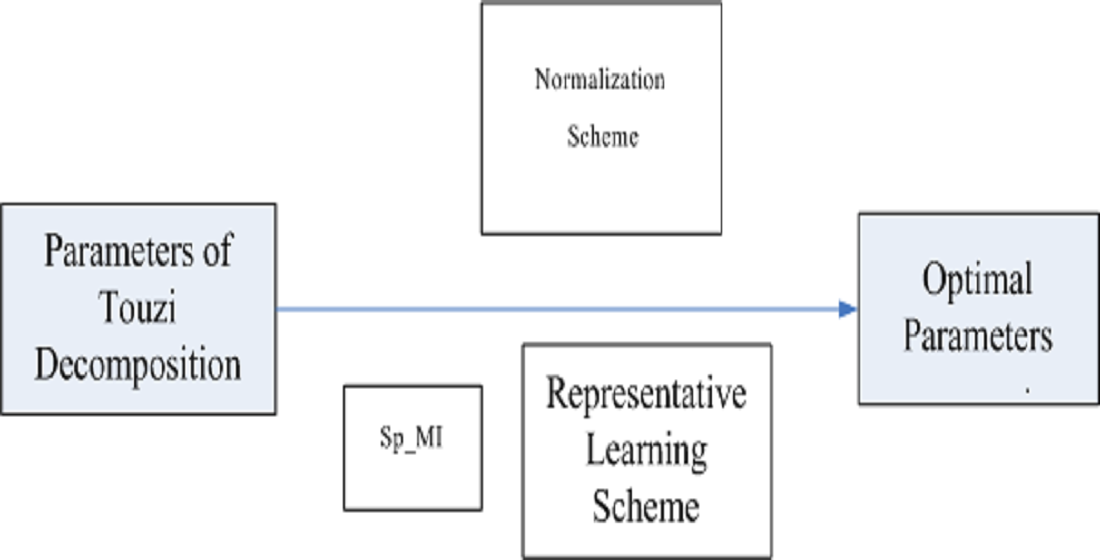
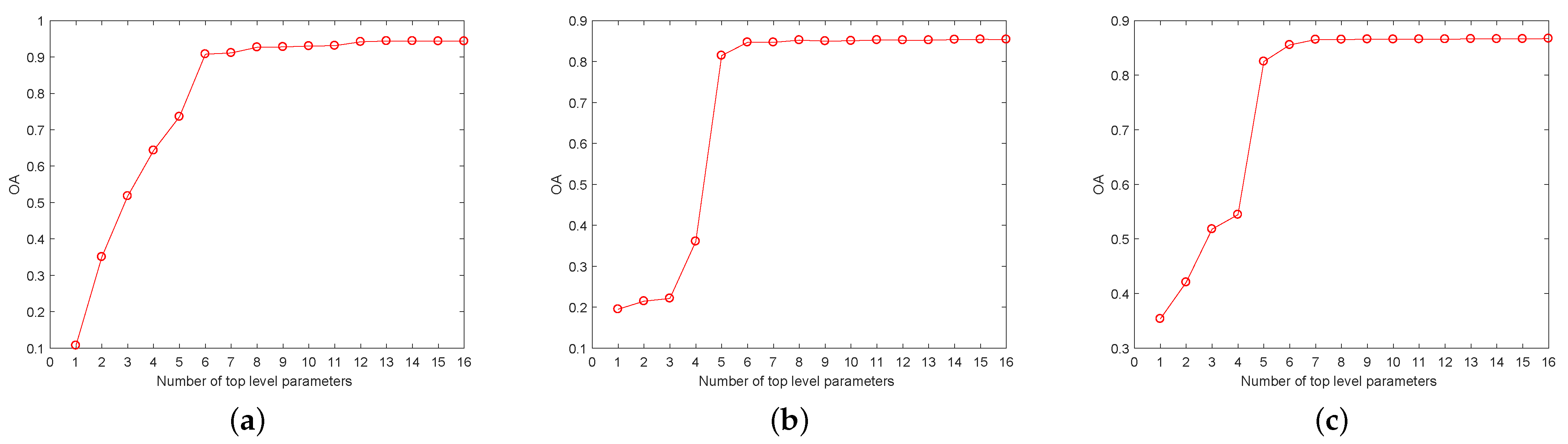
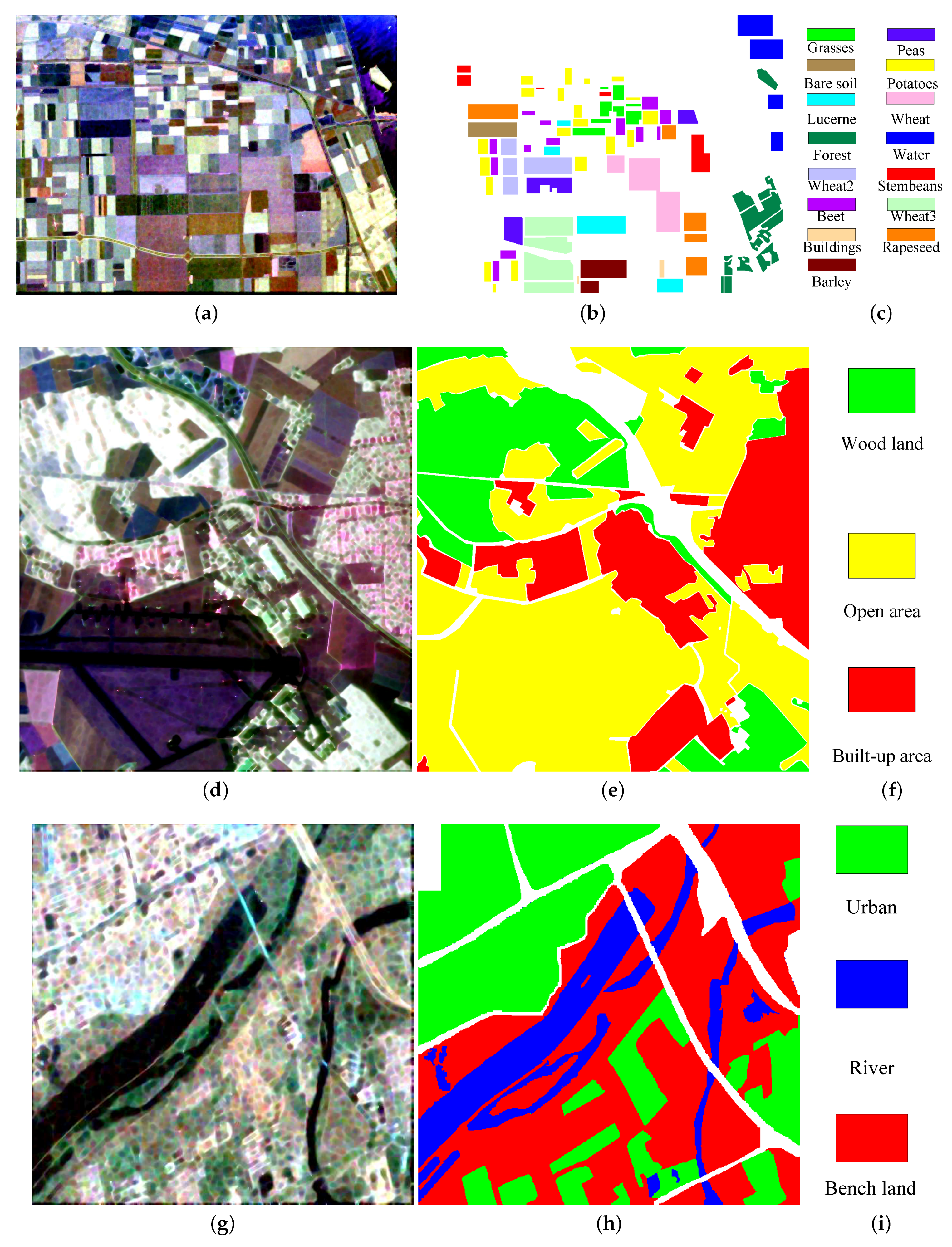
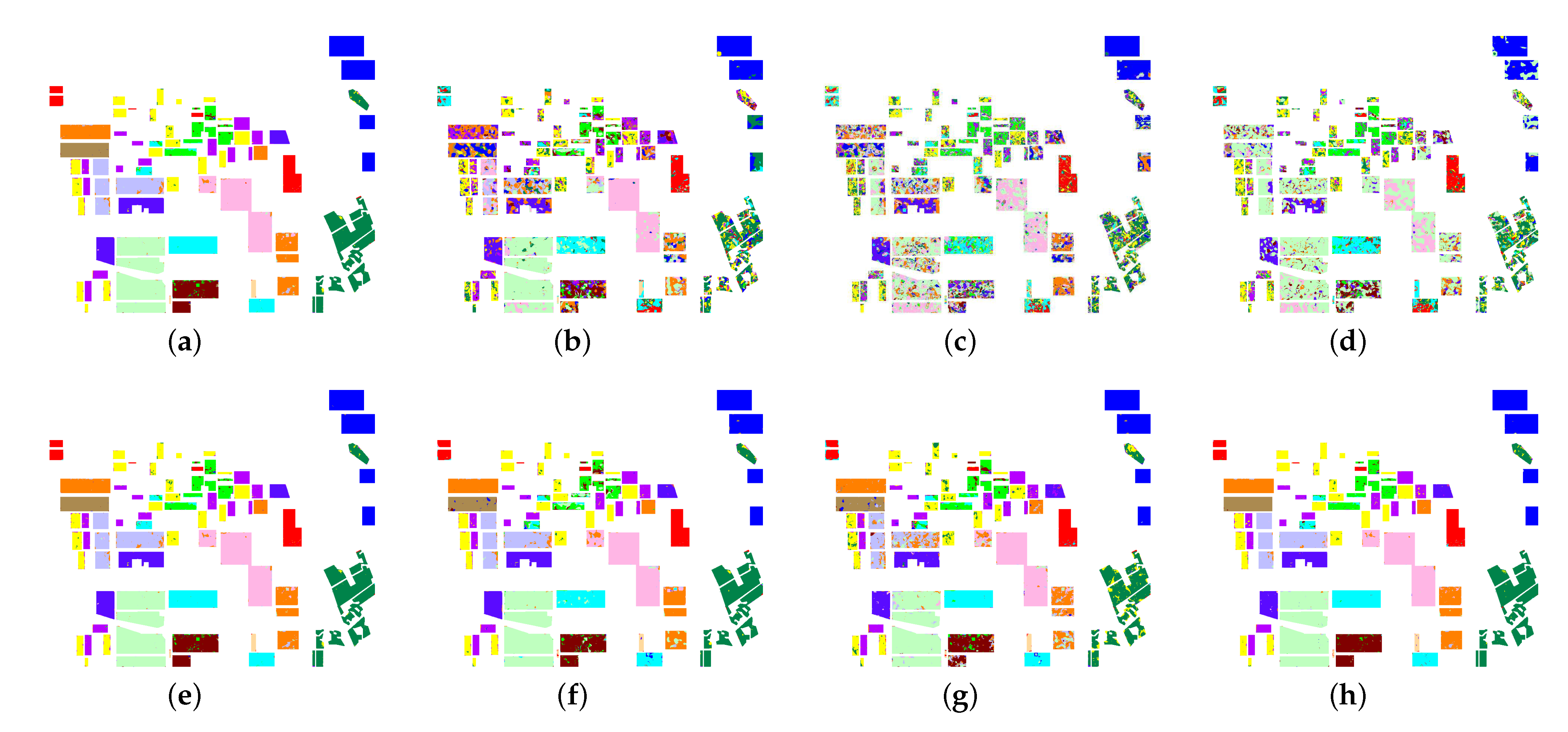
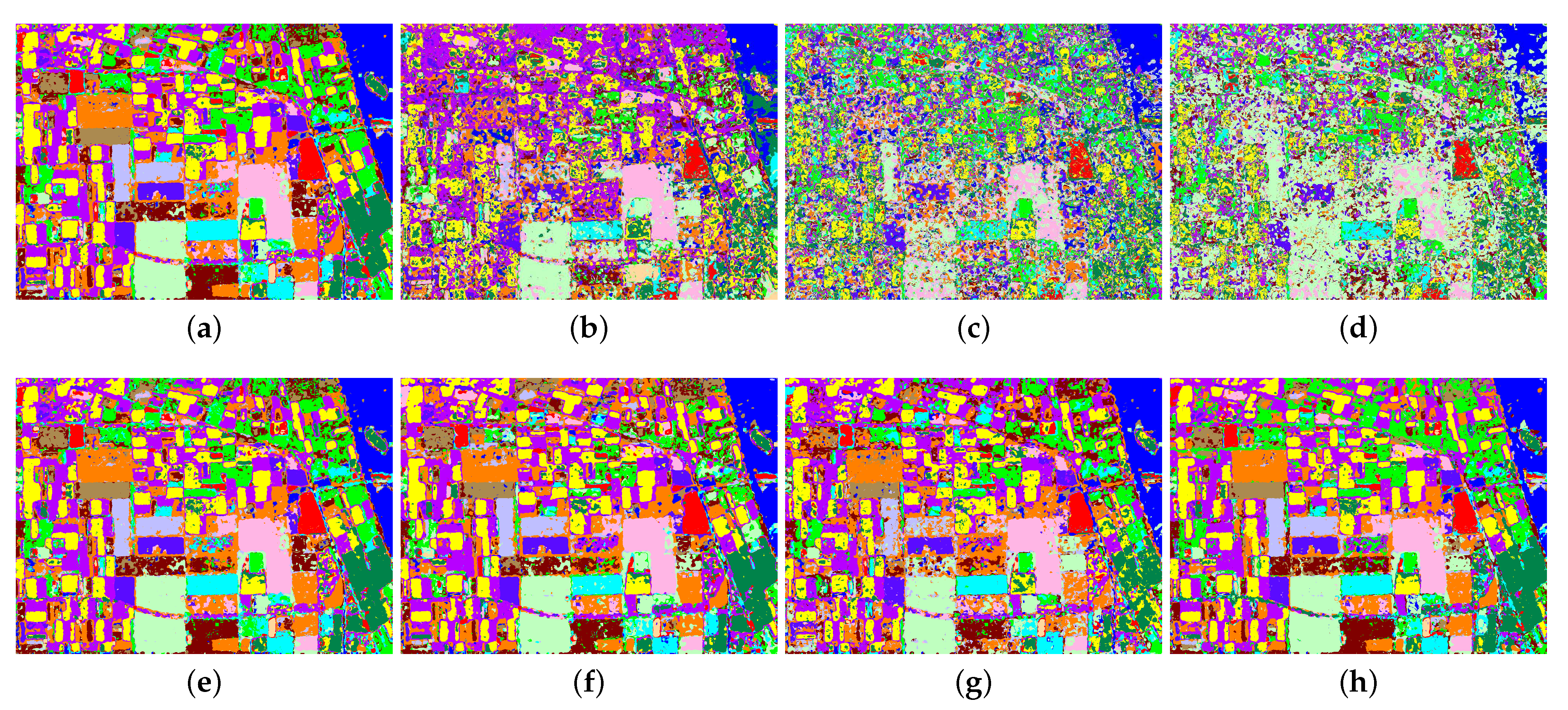
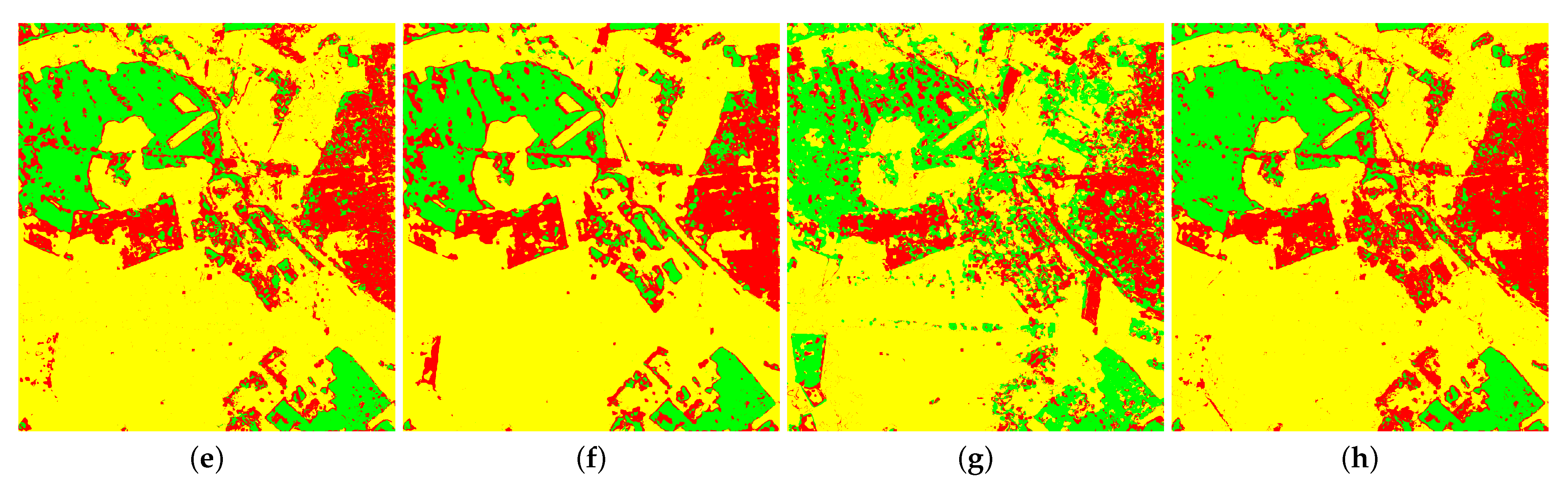
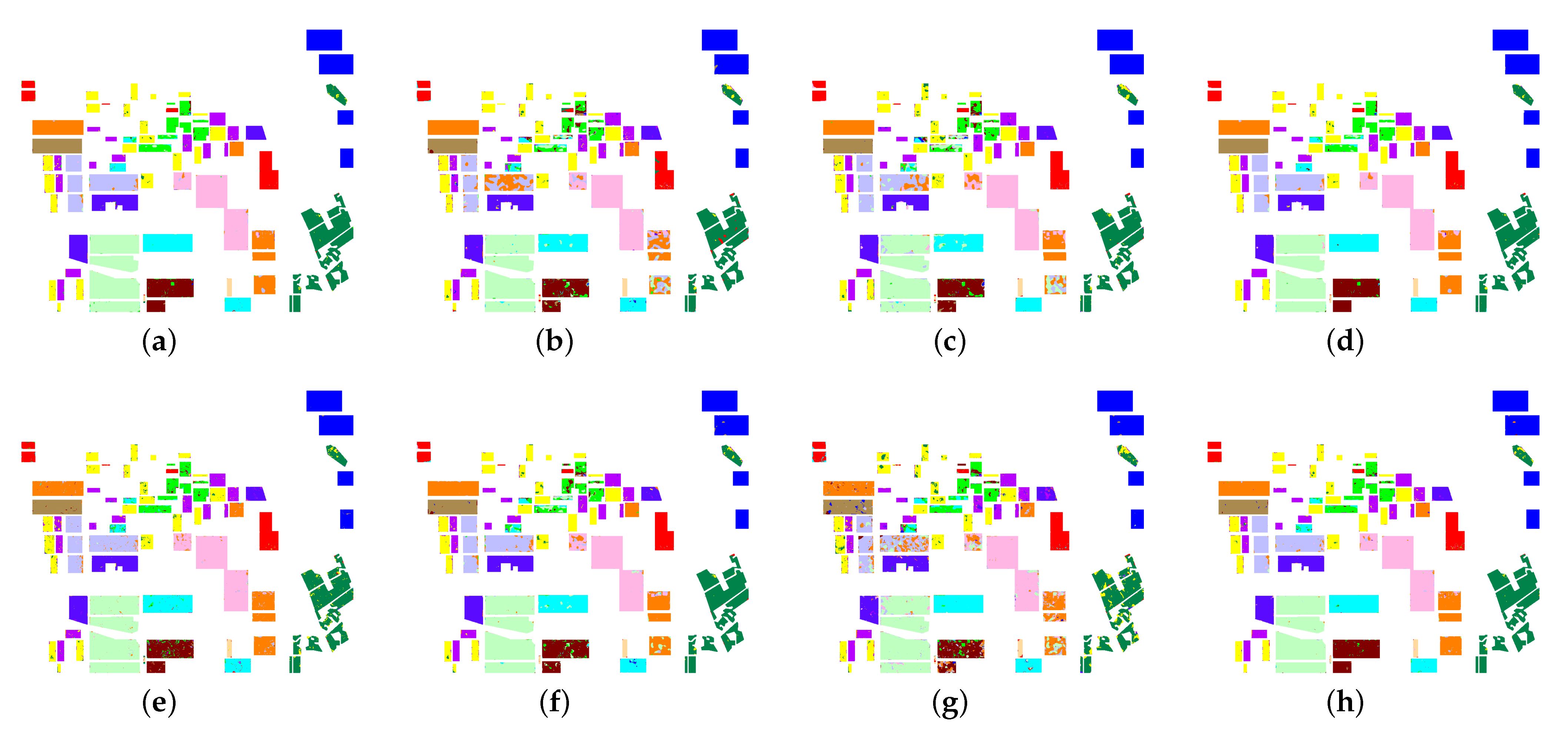
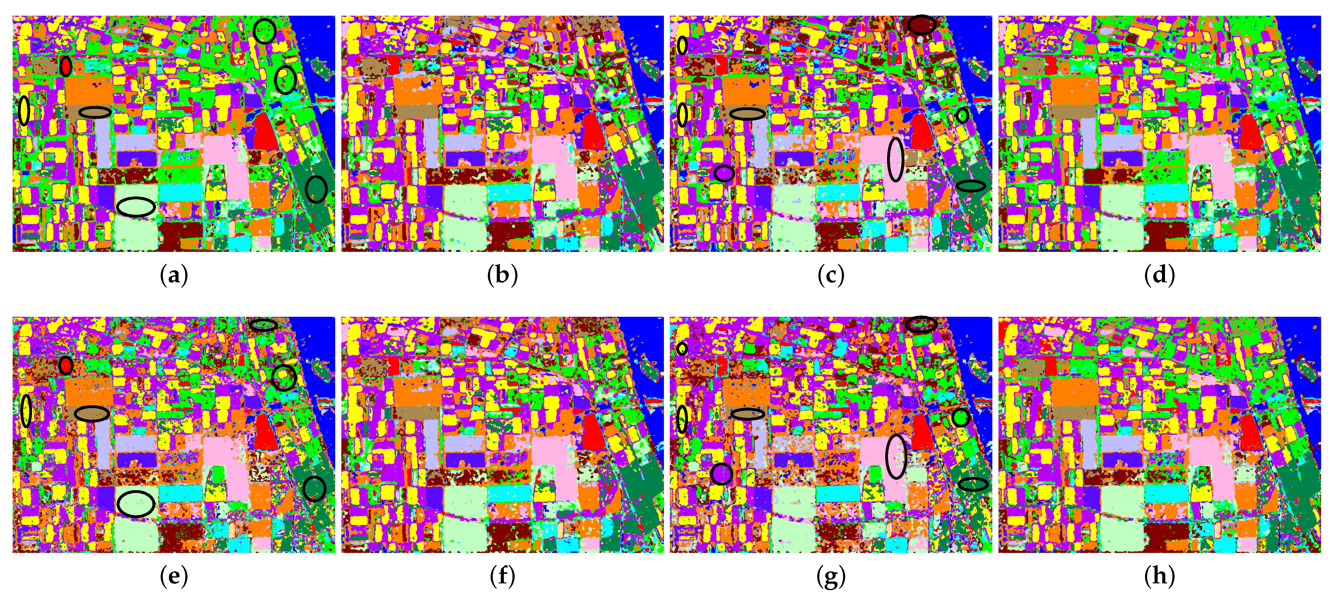
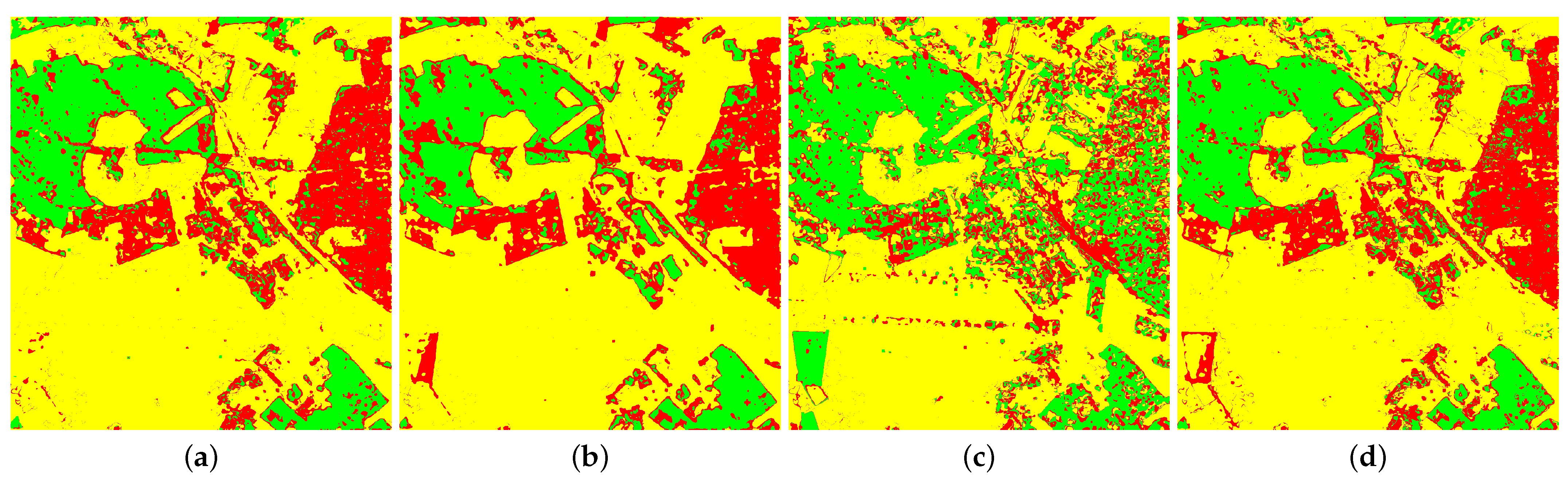
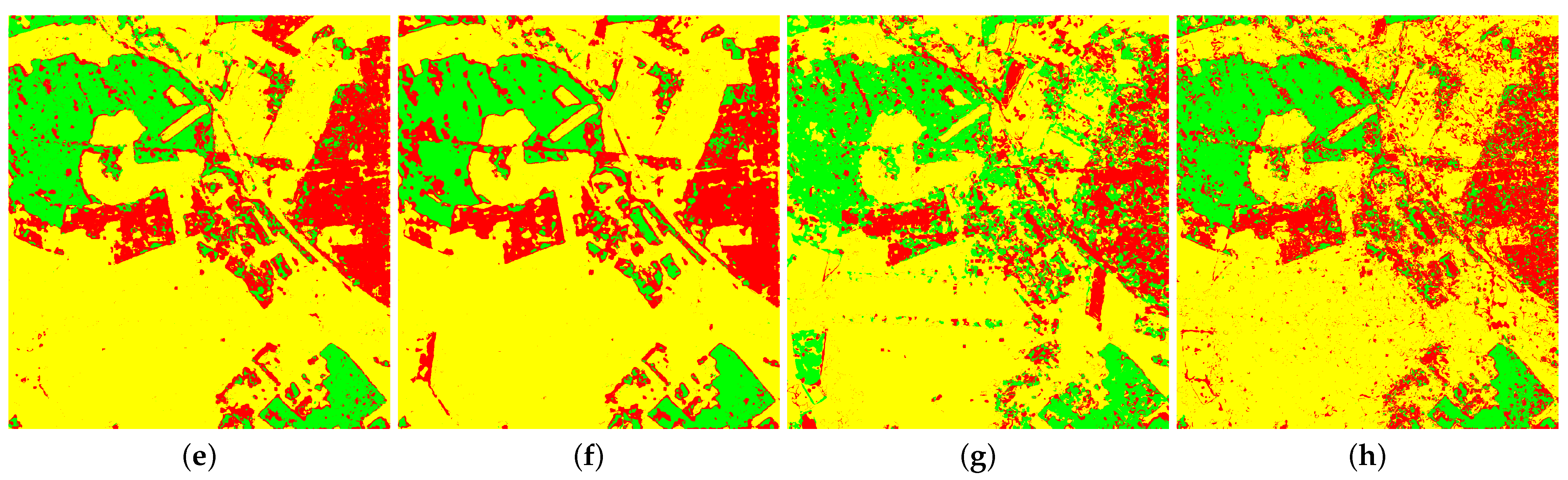
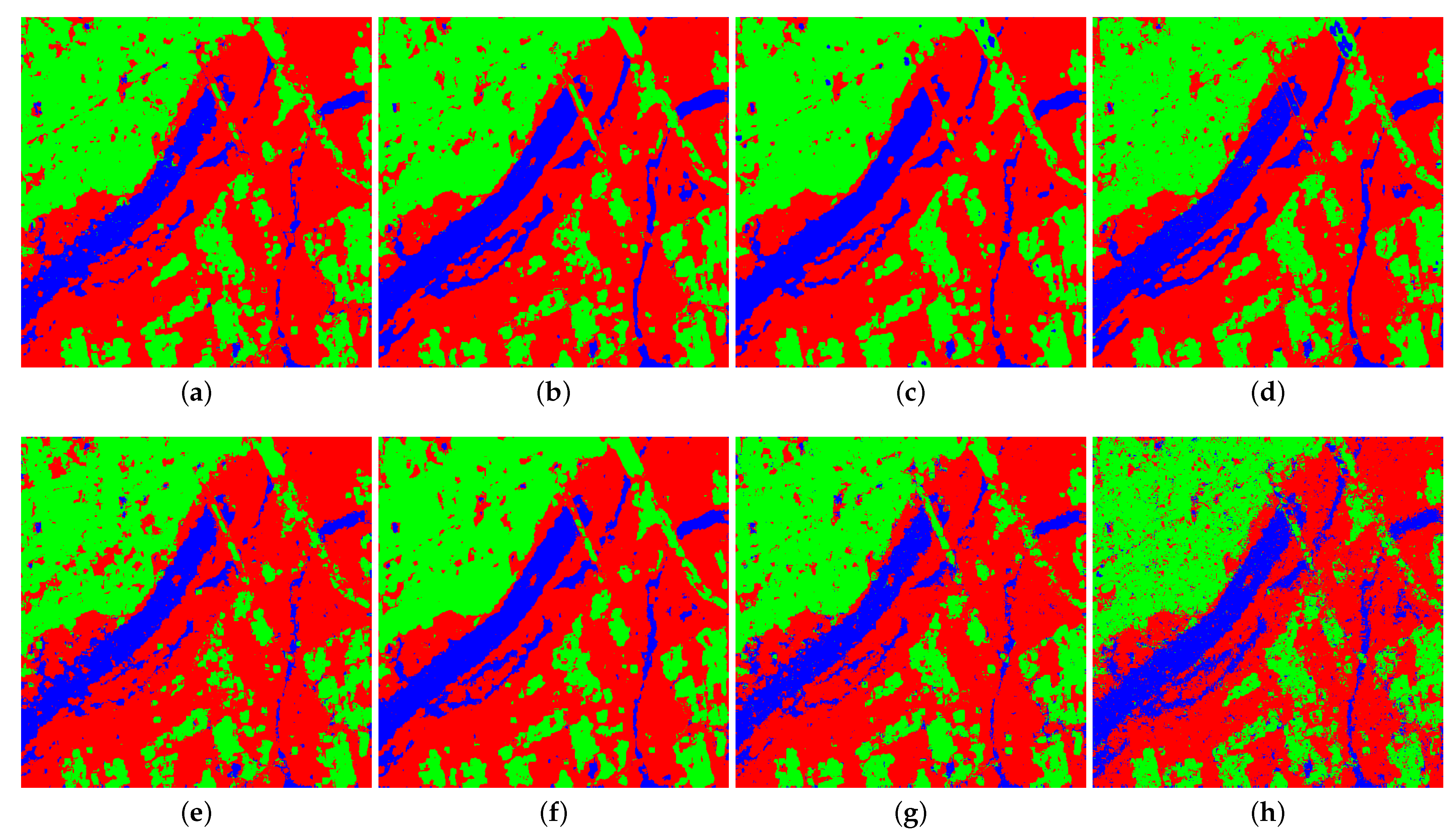
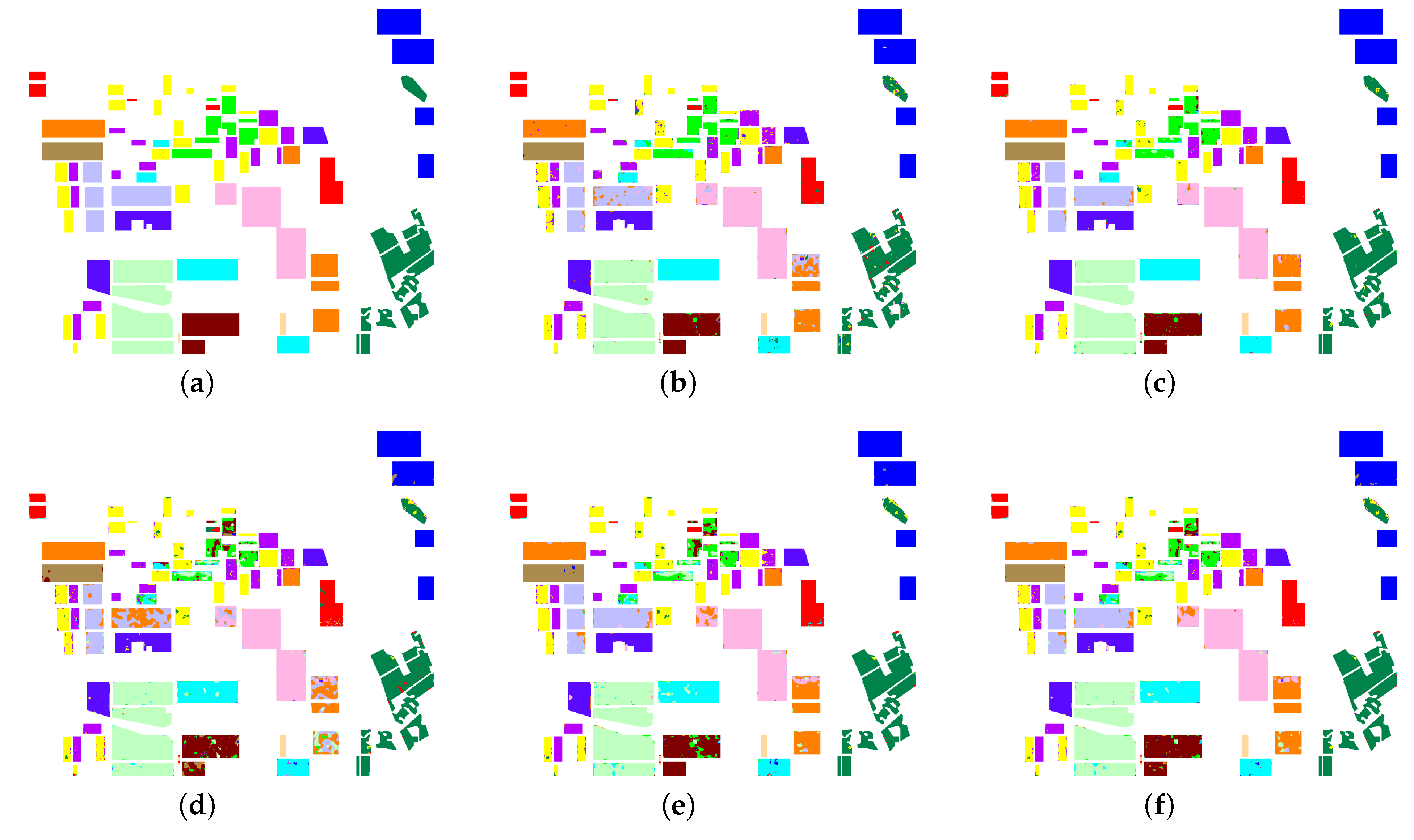
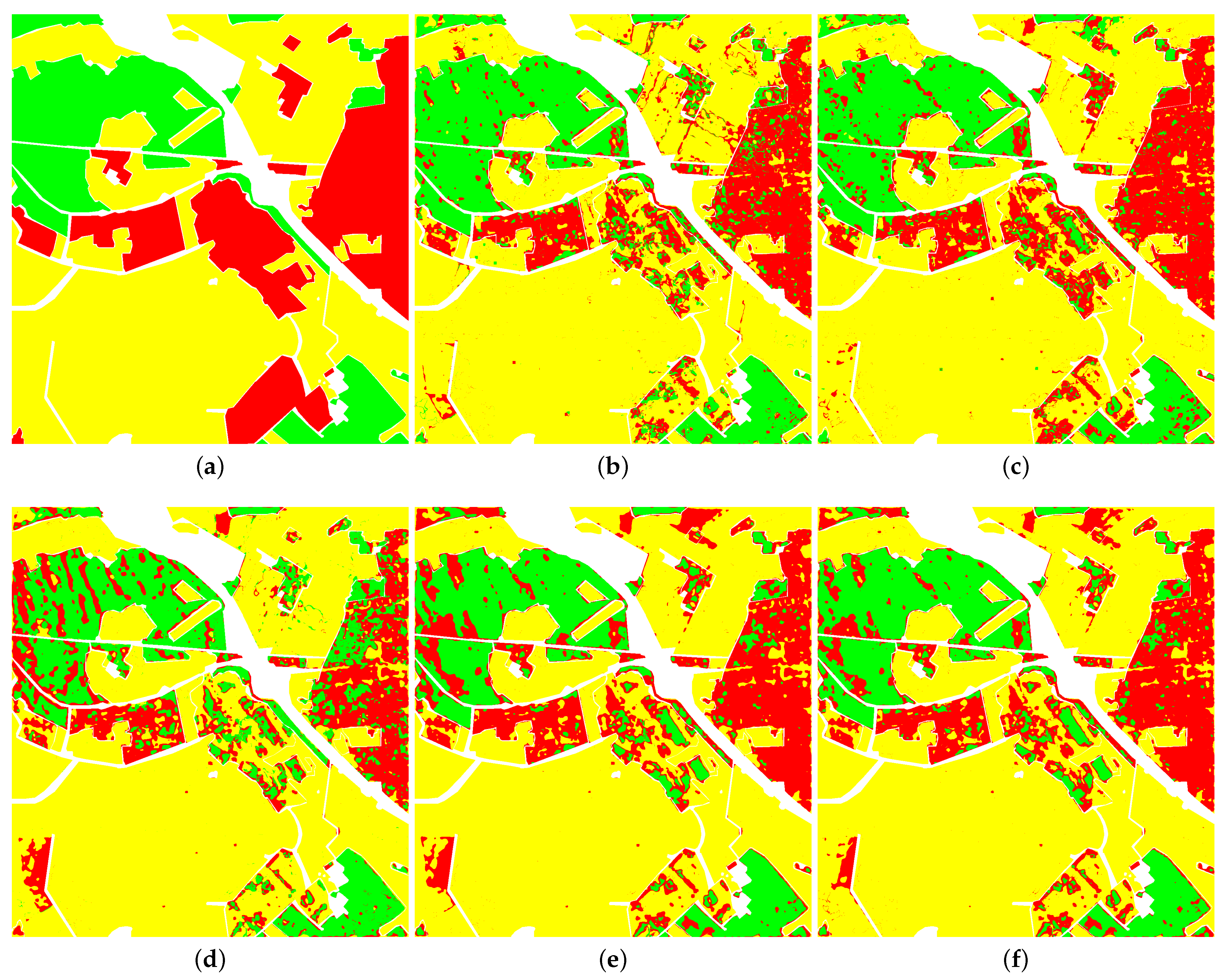
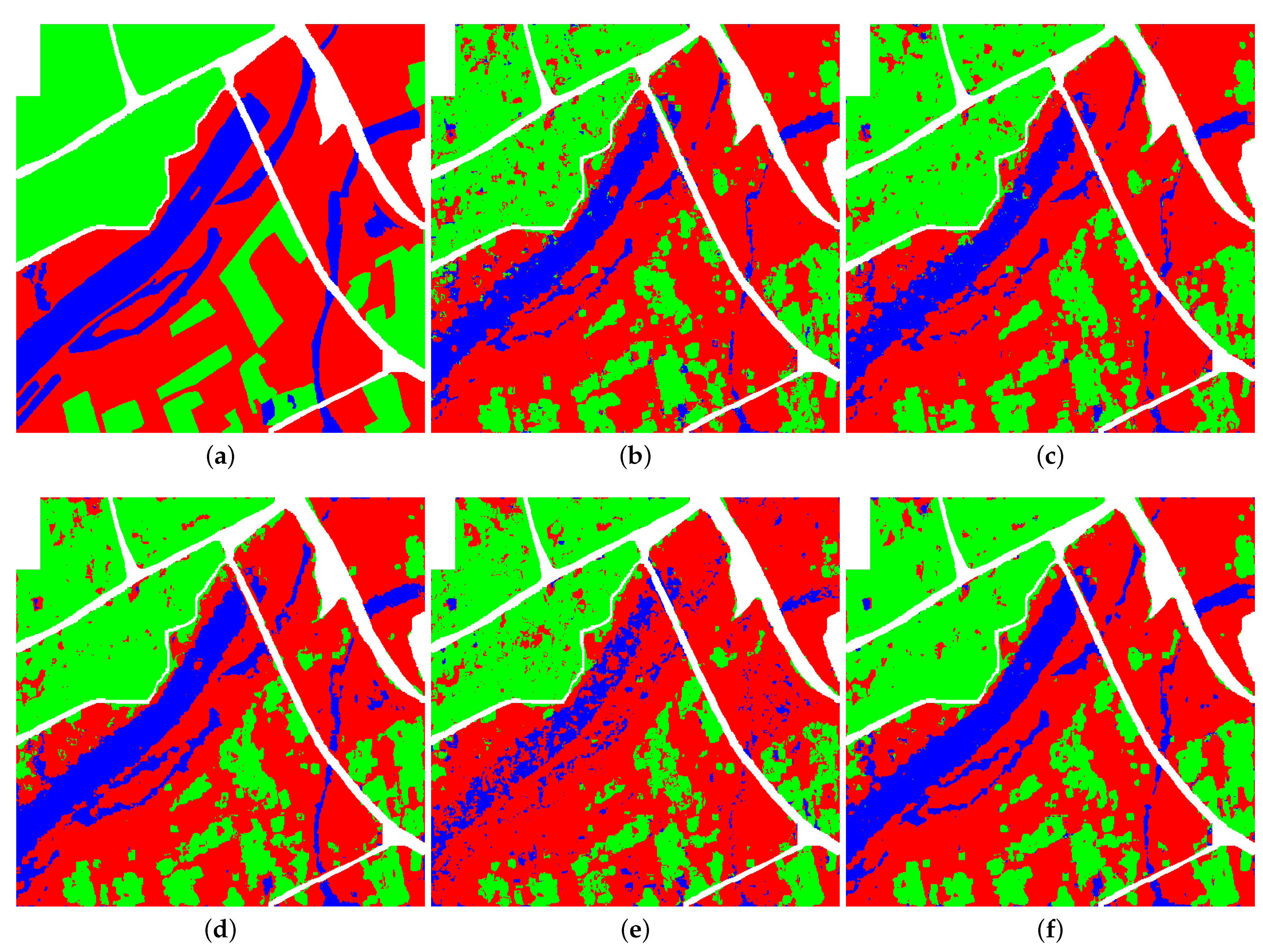
Table 1.
Parameter ranking result of Flevoland image based on different methods of mutual information.
Table 1.
Parameter ranking result of Flevoland image based on different methods of mutual information.
| MIM | MRMR | TOCD-MI | Sp-MI |
|---|---|---|---|
| span | |||
| span | span | span | |
Table 2.
Parameter ranking result of Oberpfaffenhofen image based on different methods of mutual information.
Table 2.
Parameter ranking result of Oberpfaffenhofen image based on different methods of mutual information.
| MIM | MRMR | TOCD-MI | Sp-MI |
|---|---|---|---|
| span | |||
| span | span | ||
| span | |||
Table 3.
Parameter ranking result of the Xi’an area based on different methods of mutual information.
Table 3.
Parameter ranking result of the Xi’an area based on different methods of mutual information.
| MIM | MRMR | TOCD-MI | Sp-MI |
|---|---|---|---|
| span | span | ||
| span | span | ||
Table 4.
Information on three PolSAR data sets.
| Radar | Band | Year | Resolution | Size | Categories | |
|---|---|---|---|---|---|---|
| Flevoland | AIRSAR | L | 1989 | 6.6 × 12.1 m | 750 × 1024 pixels | 15 |
| Oberpfaffenhofen | E-SAR | L | 2002 | 3.0 × 2.2 m | 1300 × 1200 pixels | 3 |
| Xi’an area | RADARSAT-2 | C | 2010 | 8 × 8 m | 512 × 512 pixels | 3 |
Table 5.
The distribution of training samples in each category for the scattering vector model (SVM) in Flevoland image.
Table 5.
The distribution of training samples in each category for the scattering vector model (SVM) in Flevoland image.
| Category | Number of Training Samples | Number of Testing Samples |
|---|---|---|
| Water | 662 | 13,232 |
| Stem beans | 317 | 6338 |
| Potatoes | 808 | 16,156 |
| Forest | 902 | 18,044 |
| Grasses | 353 | 7058 |
| Beet | 502 | 10,033 |
| Rapeseed | 693 | 13,863 |
| Peas | 479 | 9582 |
| Lucerne | 509 | 10,181 |
| Bare soil | 255 | 5109 |
| Wheat2 | 558 | 11,159 |
| Wheat | 819 | 16,386 |
| Wheat3 | 1112 | 22,241 |
| Buildings | 37 | 735 |
| Barely | 380 | 7595 |
| Total | 8386 | 167,712 |
Table 6.
The distribution of training samples in each category for the SVM in Oberpfaffenhofen image.
Table 6.
The distribution of training samples in each category for the SVM in Oberpfaffenhofen image.
| Category | Number of Training Samples | Number of Testing Samples |
|---|---|---|
| Built-up area | 268 | 267,742 |
| Wood land | 767 | 765,737 |
| Open area | 340 | 339,444 |
| Total | 1375 | 1,372,923 |
Table 7.
The distribution of training samples in each category for the SVM in Xi’an area.
| Category | Number of Training Samples | Number of Testing Samples |
|---|---|---|
| Urban | 84 | 83,862 |
| Bench land | 118 | 117,664 |
| River | 36 | 35,652 |
| Total | 238 | 237,178 |
Table 8.
Objective evaluation indicators of four classifiers on the normalized parameters and the original parameters of Touzi decomposition for Flevoland image.
Table 8.
Objective evaluation indicators of four classifiers on the normalized parameters and the original parameters of Touzi decomposition for Flevoland image.
| Water | Stem Beans | Potatoes | Forest | Grasses | Beet | |
|---|---|---|---|---|---|---|
| SVM_Ori | 0.9995 ± 0.0007 | 0.9902 ± 0.0033 | 0.9742 ± 0.0033 | 0.9781 ± 0.0039 | 0.9044 ± 0.0119 | 0.9739 ± 0.0054 |
| SVM_Uni | 0.9995 ± 0.0007 | 0.9884 ± 0.0042 | 0.9737 ± 0.0037 | 0.9776 ± 0.0036 | 0.9042 ± 0.0104 | 0.9733 ± 0.0060 |
| ANN_Ori | 0.8241 ± 0.0088 | 0.6553 ± 0.0130 | 0.6550 ± 0.0087 | 0.4859 ± 0.0100 | 0.5077 ± 0.0112 | 0.5622 ± 0.0101 |
| ANN_Uni | 0.9947 ± 0.0005 | 0.9811 ± 0.0029 | 0.9652 ± 0.0016 | 0.9763 ± 0.0016 | 0.6186 ± 0.0146 | 0.9694 ± 0.0035 |
| AE_Ori | 0.8103 ± 0.0541 | 0.5775 ± 0.0664 | 0.5753 ± 0.0633 | 0.4605 ± 0.0413 | 0.4698 ± 0.1058 | 0.2797 ± 0.0517 |
| AE_Uni | 0.9956 ± 0.0008 | 0.9574 ± 0.0077 | 0.8924 ± 0.0112 | 0.8493 ± 0.0087 | 0.7955 ± 0.0093 | 0.9182 ± 0.0092 |
| AEFT_Ori | 0.7655 ± 0.1698 | 0.6232 ± 0.0588 | 0.6593 ± 0.0486 | 0.4070 ± 0.0577 | 0.6711 ± 0.0713 | 0.4115 ± 0.0541 |
| AEFT_Uni | 0.9988 ± 0.0011 | 0.9914 ± 0.0031 | 0.9782 ± 0.0024 | 0.9854 ± 0.0023 | 0.9255 ± 0.0065 | 0.9783 ± 0.0037 |
| Rapeseed | Peas | Lucerne | Bare soil | Wheat2 | Wheat | |
| SVM_Ori | 0.9591 ± 0.0053 | 0.9908 ± 0.0031 | 0.9688 ± 0.0051 | 0.9954 ± 0.0035 | 0.9445 ± 0.0059 | 0.9731 ± 0.0036 |
| SVM_Uni | 0.9604 ± 0.0043 | 0.9899 ± 0.0029 | 0.9663 ± 0.0064 | 0.9954 ± 0.0033 | 0.9455 ± 0.0057 | 0.9724 ± 0.0042 |
| ANN_Ori | 0.4743 ± 0.0098 | 0.6921 ± 0.0107 | 0.5854 ± 0.0128 | 0.2282 ± 0.0194 | 0.3448 ± 0.0316 | 0.8467 ± 0.0033 |
| ANN_Uni | 0.9221 ± 0.0026 | 0.9864 ± 0.0017 | 0.8944 ± 0.0042 | 0.9619 ± 0.0074 | 0.9230 ± 0.0031 | 0.9508 ± 0.0033 |
| AE_Ori | 0.2720 ± 0.0669 | 0.5524 ± 0.0511 | 0.4914 ± 0.0807 | 0.2592 ± 0.0584 | 0.0541 ± 0.0454 | 0.5805 ± 0.1055 |
| AE_Uni | 0.8073 ± 0.0218 | 0.9490 ± 0.0086 | 0.9132 ± 0.0047 | 0.9333 ± 0.0126 | 0.7220 ± 0.0222 | 0.9020 ± 0.0090 |
| AEFT_Ori | 0.2496 ± 0.0637 | 0.5406 ± 0.0742 | 0.6453 ± 0.0663 | 0.2230 ± 0.0677 | 0.0610 ± 0.0518 | 0.4286 ± 0.2283 |
| AEFT_Uni | 0.9678 ± 0.0033 | 0.9913 ± 0.0021 | 0.9830 ± 0.0034 | 0.9966 ± 0.0023 | 0.9602 ± 0.0028 | 0.9777 ± 0.0029 |
| Wheat3 | Buildings | Barely | OA | |||
| SVM_Ori | 0.9929 ± 0.0018 | 0.9411 ± 0.0268 | 0.9403 ± 0.0099 | 0.9730 ± 0.0012 | ||
| SVM_Uni | 0.9925 ± 0.0019 | 0.9421 ± 0.0256 | 0.9404 ± 0.0078 | 0.9726 ± 0.0009 | ||
| ANN_Ori | 0.8899 ± 0.0028 | 0.5054 ± 0.0961 | 0.4296 ± 0.0165 | 0.6267 ± 0.0034 | ||
| ANN_Uni | 0.9890 ± 0.0012 | 0.9621 ± 0.0112 | 0.9056 ± 0.0066 | 0.9445 ± 0.0010 | ||
| AE_Ori | 0.4576 ± 0.1018 | 0.1031 ± 0.1194 | 0.1341 ± 0.0574 | 0.4465 ± 0.0186 | ||
| AE_Uni | 0.9466 ± 0.0059 | 0.8549 ± 0.0550 | 0.7801 ± 0.0227 | 0.8861 ± 0.0048 | ||
| AEFT_Ori | 0.7154 ± 0.1477 | 0.1911 ± 0.2031 | 0.2733 ± 0.0761 | 0.4956 ± 0.0223 | ||
| AEFT_Uni | 0.9946 ± 0.0012 | 0.9500 ± 0.0222 | 0.9767 ± 0.0053 | 0.9804 ± 0.0007 |
Table 9.
Objective evaluation indicators of four classifiers on the normalized parameters and the original parameters of Touzi decomposition for Oberpfaffenhofen image.
Table 9.
Objective evaluation indicators of four classifiers on the normalized parameters and the original parameters of Touzi decomposition for Oberpfaffenhofen image.
| Built-Up Area | Wood Land | Open Area | OA | |
|---|---|---|---|---|
| SVM_Ori | 0.8385 ± 0.0174 | 0.9663 ± 0.0087 | 0.6849 ± 0.0193 | 0.8718 ± 0.0045 |
| SVM_Uni | 0.8407 ± 0.0144 | 0.9663 ± 0.0096 | 0.6774 ± 0.0181 | 0.8704 ± 0.0051 |
| ANN_Ori | 0.7766 ± 0.0070 | 0.9691 ± 0.0015 | 0.6681 ± 0.0048 | 0.8571 ± 0.0013 |
| ANN_Uni | 0.7834 ± 0.0077 | 0.9752 ± 0.0011 | 0.6387 ± 0.0039 | 0.8546 ± 0.0010 |
| AE_Ori | 0.6484 ± 0.0517 | 0.8819 ± 0.0108 | 0.3581 ± 0.0469 | 0.7069 ± 0.0096 |
| AE_Uni | 0.7673 ± 0.0120 | 0.8417 ± 0.0065 | 0.4682 ± 0.0111 | 0.7349 ± 0.0048 |
| AEFT_Ori | 0.6493 ± 0.0801 | 0.9290 ± 0.0449 | 0.4177 ± 0.1147 | 0.7481 ± 0.0189 |
| AEFT_Uni | 0.8823 ± 0.0043 | 0.9704 ± 0.0021 | 0.7512 ± 0.0046 | 0.8990 ± 0.0014 |
Table 10.
Objective evaluation indicators of four classifiers on the normalized parameters and the original parameters of Touzi decomposition for Xi’an area.
Table 10.
Objective evaluation indicators of four classifiers on the normalized parameters and the original parameters of Touzi decomposition for Xi’an area.
| Urban | Bench Land | River | OA | |
|---|---|---|---|---|
| SVM_Ori | 0.8653 ± 0.0222 | 0.8822 ± 0.0192 | 0.6290 ± 0.0750 | 0.8382 ± 0.0124 |
| SVM_Uni | 0.8616 ± 0.0262 | 0.8798 ± 0.0204 | 0.6205 ± 0.0748 | 0.8344 ± 0.0138 |
| ANN_Ori | 0.8578 ± 0.0029 | 0.9004 ± 0.0023 | 0.7696 ± 0.0157 | 0.8657 ± 0.0021 |
| ANN_Uni | 0.8564 ± 0.0034 | 0.9026 ± 0.0021 | 0.7729 ± 0.0106 | 0.8668 ± 0.0016 |
| AE_Ori | 0.6696 ± 0.0435 | 0.8738 ± 0.0182 | 0.0962 ± 0.0227 | 0.6847 ± 0.0111 |
| AE_Uni | 0.8811 ± 0.0098 | 0.8942 ± 0.0040 | 0.6969 ± 0.0453 | 0.8599 ± 0.0096 |
| AEFT_Ori | 0.6235 ± 0.0651 | 0.8969 ± 0.0073 | 0.2013 ± 0.0483 | 0.6956 ± 0.0251 |
| AEFT_Uni | 0.9081 ± 0.0031 | 0.8926 ± 0.0023 | 0.8313 ± 0.0046 | 0.8889 ± 0.0009 |
Table 11.
Objective evaluation indicators of four classifiers on the learned parameters and all parameters of Touzi decomposition for the Flevoland image.
Table 11.
Objective evaluation indicators of four classifiers on the learned parameters and all parameters of Touzi decomposition for the Flevoland image.
| Water | Stem Beans | Potatoes | Forest | Grasses | Beet | |
|---|---|---|---|---|---|---|
| SVM_LP | 1.0000 ± 0.0001 | 0.9928 ± 0.0046 | 0.9737 ± 0.0035 | 0.9809 ± 0.0036 | 0.8992 ± 0.0145 | 0.9814 ± 0.0056 |
| SVM_AP | 0.9986 ± 0.0011 | 0.9759 ± 0.0063 | 0.9457 ± 0.0060 | 0.9431 ± 0.0056 | 0.8750 ± 0.0098 | 0.9373 ± 0.0063 |
| ANN_LP | 0.9934 ± 0.0021 | 0.9748 ± 0.0050 | 0.9621 ± 0.0028 | 0.9729 ± 0.0020 | 0.6140 ± 0.0267 | 0.9611 ± 0.0043 |
| ANN_AP | 0.9948 ± 0.0010 | 0.9777 ± 0.0044 | 0.9639 ± 0.0031 | 0.9752 ± 0.0019 | 0.6151 ± 0.0196 | 0.9666 ± 0.0046 |
| AE_LP | 0.9999 ± 0.0001 | 0.9784 ± 0.0033 | 0.9407 ± 0.0140 | 0.9480 ± 0.0103 | 0.6185 ± 0.0130 | 0.9624 ± 0.0055 |
| AE_AP | 0.9950 ± 0.0010 | 0.9523 ± 0.0107 | 0.8882 ± 0.0128 | 0.8451 ± 0.0100 | 0.7887 ± 0.0142 | 0.9109 ± 0.0114 |
| AEFT_LP | 0.9990 ± 0.0013 | 0.9874 ± 0.0057 | 0.9741 ± 0.0035 | 0.9821 ± 0.0032 | 0.8731 ± 0.0097 | 0.9806 ± 0.0036 |
| AEFT_AP | 0.9980 ± 0.0016 | 0.9846 ± 0.0058 | 0.9699 ± 0.0029 | 0.9800 ± 0.0029 | 0.8979 ± 0.0121 | 0.9638 ± 0.0076 |
| Rapeseed | Peas | Lucerne | Bare soil | Wheat2 | Wheat | |
| SVM_LP | 0.9654 ± 0.0037 | 0.9889 ± 0.0034 | 0.9732 ± 0.0063 | 0.9988 ± 0.0007 | 0.9597 ± 0.0034 | 0.9787 ± 0.0026 |
| SVM_AP | 0.9425 ± 0.0056 | 0.9749 ± 0.0033 | 0.9433 ± 0.0071 | 0.9803 ± 0.0078 | 0.9342 ± 0.0076 | 0.9653 ± 0.0037 |
| ANN_LP | 0.9263 ± 0.0035 | 0.9750 ± 0.0018 | 0.8848 ± 0.0081 | 0.9946 ± 0.0008 | 0.9239 ± 0.0032 | 0.9484 ± 0.0033 |
| ANN_AP | 0.9220 ± 0.0038 | 0.9851 ± 0.0021 | 0.8938 ± 0.0057 | 0.9607 ± 0.0092 | 0.9240 ± 0.0053 | 0.9492 ± 0.0049 |
| AE_LP | 0.8072 ± 0.0159 | 0.9624 ± 0.0046 | 0.8476 ± 0.0059 | 0.9959 ± 0.0010 | 0.8765 ± 0.0230 | 0.9420 ± 0.0069 |
| AE_AP | 0.8030 ± 0.0170 | 0.9478 ± 0.0098 | 0.9136 ± 0.0061 | 0.9340 ± 0.0148 | 0.7141 ± 0.0343 | 0.9036 ± 0.0102 |
| AEFT_LP | 0.9611 ± 0.0060 | 0.9810 ± 0.0033 | 0.9799 ± 0.0051 | 0.9984 ± 0.0011 | 0.9551 ± 0.0034 | 0.9767 ± 0.0023 |
| AEFT_AP | 0.9613 ± 0.0049 | 0.9876 ± 0.0040 | 0.9732 ± 0.0048 | 0.9947 ± 0.0034 | 0.9579 ± 0.0048 | 0.9755 ± 0.0039 |
| Wheat3 | Buildings | Barely | OA | |||
| SVM_LP | 0.9905 ± 0.0017 | 0.9733 ± 0.0153 | 0.9682 ± 0.0052 | 0.9770 ± 0.0010 | ||
| SVM_AP | 0.9841 ± 0.0024 | 0.9039 ± 0.0275 | 0.9050 ± 0.0110 | 0.9538 ± 0.0013 | ||
| ANN_LP | 0.9817 ± 0.0017 | 0.9322 ± 0.0276 | 0.9399 ± 0.0074 | 0.9432 ± 0.0015 | ||
| ANN_AP | 0.9882 ± 0.0013 | 0.9488 ± 0.0224 | 0.9015 ± 0.0106 | 0.9432 ± 0.0014 | ||
| AE_LP | 0.9547 ± 0.0037 | 0.9053 ± 0.0190 | 0.8621 ± 0.0114 | 0.9516 ± 0.0049 | ||
| AE_AP | 0.9453 ± 0.0070 | 0.8333 ± 0.0776 | 0.7775 ± 0.0259 | 0.8831 ± 0.0066 | ||
| AEFT_LP | 0.9891 ± 0.0016 | 0.9487 ± 0.0292 | 0.9750 ± 0.0042 | 0.9749 ± 0.0007 | ||
| AEFT_AP | 0.9932 ± 0.0019 | 0.9153 ± 0.0506 | 0.9638 ± 0.0078 | 0.9739 ± 0.0014 |
Table 12.
Objective evaluation indicators of four classifiers on the learned parameters and all parameters of Touzi decomposition for Oberpfaffenhofen image.
Table 12.
Objective evaluation indicators of four classifiers on the learned parameters and all parameters of Touzi decomposition for Oberpfaffenhofen image.
| Built-Up Area | Wood Land | Open Area | OA | |
|---|---|---|---|---|
| SVM_LP | 0.8357 ± 0.0180 | 0.9733 ± 0.0048 | 0.6807 ± 0.0157 | 0.8741 ± 0.0050 |
| SVM_AP | 0.8381 ± 0.0210 | 0.9686 ± 0.0072 | 0.6672 ± 0.0192 | 0.8686 ± 0.0054 |
| ANN_LP | 0.7488 ± 0.0180 | 0.9733 ± 0.0048 | 0.6542 ± 0.0110 | 0.8506 ± 0.0028 |
| ANN_AP | 0.7752 ± 0.0202 | 0.9730 ± 0.0049 | 0.6342 ± 0.0140 | 0.8507 ± 0.0032 |
| AE_LP | 0.6608 ± 0.0664 | 0.8477 ± 0.0113 | 0.3981 ± 0.0485 | 0.7001 ± 0.0072 |
| AE_AP | 0.7497 ± 0.0214 | 0.8448 ± 0.0123 | 0.4576 ± 0.0230 | 0.7305 ± 0.0064 |
| AEFT_LP | 0.8442 ± 0.0124 | 0.9557 ± 0.0062 | 0.6987 ± 0.0142 | 0.8704 ± 0.0048 |
| AEFT_AP | 0.8015 ± 0.0135 | 0.9087 ± 0.0104 | 0.6373 ± 0.0159 | 0.8207 ± 0.0071 |
Table 13.
Objective evaluation indicators of four classifiers on the learned parameters and all parameters of Touzi decomposition for Xi’an area.
Table 13.
Objective evaluation indicators of four classifiers on the learned parameters and all parameters of Touzi decomposition for Xi’an area.
| Urban | Bench Land | River | OA | |
|---|---|---|---|---|
| SVM_LP | 0.8841 ± 0.0227 | 0.8837 ± 0.0250 | 0.7262 ± 0.0726 | 0.8602 ± 0.0104 |
| SVM_AP | 0.8531 ± 0.0217 | 0.8892 ± 0.0170 | 0.6100 ± 0.0712 | 0.8345 ± 0.0105 |
| ANN_LP | 0.8542 ± 0.0094 | 0.9021 ± 0.0055 | 0.7588 ± 0.0286 | 0.8636 ± 0.0039 |
| ANN_AP | 0.8542 ± 0.0084 | 0.9004 ± 0.0048 | 0.7680 ± 0.0241 | 0.8642 ± 0.0028 |
| AE_LP | 0.8979 ± 0.0052 | 0.9018 ± 0.0048 | 0.7893 ± 0.0197 | 0.8835 ± 0.0018 |
| AE_AP | 0.8775 ± 0.0097 | 0.8916 ± 0.0061 | 0.6779 ± 0.0402 | 0.8545 ± 0.0079 |
| AEFT_LP | 0.8906 ± 0.0063 | 0.8924 ± 0.0051 | 0.8265 ± 0.0096 | 0.8819 ± 0.0024 |
| AEFT_AP | 0.8508 ± 0.0078 | 0.8489 ± 0.0079 | 0.7709 ± 0.0153 | 0.8379 ± 0.0042 |
Table 14.
The objective indicators of three ANN-based classifiers and two SVM classifiers on different forms of parameters of Touzi decomposition for the Flevoland image.
Table 14.
The objective indicators of three ANN-based classifiers and two SVM classifiers on different forms of parameters of Touzi decomposition for the Flevoland image.
| SVM_PP | SVM_LP | ANN_Opt | ANN_MIM | ANN_SpMI | |
|---|---|---|---|---|---|
| Water | 0.9987 ± 0.0011 | 1.0000 ± 0.0001 | 0.9931 ± 0.0015 | 0.9951 ± 0.0009 | 0.9938 ± 0.0017 |
| Stem beans | 0.9520 ± 0.0080 | 0.9928 ± 0.0046 | 0.9105 ± 0.0065 | 0.9721 ± 0.0061 | 0.9755 ± 0.0035 |
| Potatoes | 0.9482 ± 0.0048 | 0.9737 ± 0.0035 | 0.9544 ± 0.0028 | 0.9568 ± 0.0032 | 0.9607 ± 0.0031 |
| Forest | 0.9333 ± 0.0062 | 0.9809 ± 0.0036 | 0.9603 ± 0.0029 | 0.9709 ± 0.0030 | 0.9735 ± 0.0025 |
| Grasses | 0.9219 ± 0.0090 | 0.8992 ± 0.0145 | 0.5762 ± 0.0261 | 0.6183 ± 0.0253 | 0.6286 ± 0.0280 |
| Beet | 0.9319 ± 0.0101 | 0.9814 ± 0.0056 | 0.9394 ± 0.0060 | 0.9616 ± 0.0030 | 0.9614 ± 0.0040 |
| Rapeseed | 0.8885 ± 0.0096 | 0.9654 ± 0.0037 | 0.7618 ± 0.0132 | 0.9230 ± 0.0038 | 0.9265 ± 0.0041 |
| Peas | 0.9793 ± 0.0045 | 0.9889 ± 0.0034 | 0.9712 ± 0.0026 | 0.9688 ± 0.0018 | 0.9756 ± 0.0019 |
| Lucerne | 0.9594 ± 0.0086 | 0.9732 ± 0.0063 | 0.8897 ± 0.0058 | 0.8638 ± 0.0090 | 0.8836 ± 0.0087 |
| Bare soil | 0.9956 ± 0.0030 | 0.9988 ± 0.0007 | 0.9731 ± 0.0034 | 0.9875 ± 0.0056 | 0.9945 ± 0.0005 |
| Wheat2 | 0.9108 ± 0.0091 | 0.9597 ± 0.0034 | 0.6853 ± 0.0235 | 0.9197 ± 0.0022 | 0.9231 ± 0.0031 |
| Wheat | 0.9633 ± 0.0035 | 0.9787 ± 0.0026 | 0.9381 ± 0.0052 | 0.9358 ± 0.0057 | 0.9485 ± 0.0038 |
| Wheat3 | 0.9935 ± 0.0019 | 0.9905 ± 0.0017 | 0.9893 ± 0.0014 | 0.9778 ± 0.0017 | 0.9819 ± 0.0021 |
| Buildings | 0.9531 ± 0.0270 | 0.9733 ± 0.0153 | 0.9335 ± 0.0191 | 0.9404 ± 0.0187 | 0.9327 ± 0.0368 |
| Barely | 0.9677 ± 0.0061 | 0.9682 ± 0.0052 | 0.8913 ± 0.0123 | 0.8696 ± 0.0187 | 0.9353 ± 0.0101 |
| OA | 0.9535 ± 0.0014 | 0.9770 ± 0.0010 | 0.9035 ± 0.0012 | 0.9354 ± 0.0013 | 0.9435 ± 0.0013 |
Table 15.
The objective indicators of three ANN-based classifiers and two SVM classifiers on different forms of parameters of Touzi decomposition for the Oberpfaffenhofen image.
Table 15.
The objective indicators of three ANN-based classifiers and two SVM classifiers on different forms of parameters of Touzi decomposition for the Oberpfaffenhofen image.
| SVM_PP | SVM_LP | ANN_Opt | ANN_MIM | ANN_SpMI | |
|---|---|---|---|---|---|
| Wood land | 0.8575 ± 0.0144 | 0.8357 ± 0.0180 | 0.7033 ± 0.0270 | 0.7412 ± 0.0163 | 0.7557 ± 0.0179 |
| Open area | 0.9629 ± 0.0107 | 0.9733 ± 0.0048 | 0.9713 ± 0.0061 | 0.9724 ± 0.0038 | 0.9743 ± 0.0040 |
| Built-up area | 0.6475 ± 0.0245 | 0.6807 ± 0.0157 | 0.5120 ± 0.0135 | 0.6491 ± 0.0096 | 0.6511 ± 0.0132 |
| OA | 0.8644 ± 0.0043 | 0.8741 ± 0.0050 | 0.8055 ± 0.0043 | 0.8474 ± 0.0024 | 0.8518 ± 0.0024 |
Table 16.
The objective indicators of three ANN-based classifiers and two SVM classifiers on different forms of parameters of Touzi decomposition for the Xian area.
Table 16.
The objective indicators of three ANN-based classifiers and two SVM classifiers on different forms of parameters of Touzi decomposition for the Xian area.
| SVM_PP | SVM_LP | ANN_Opt | ANN_MIM | ANN_SpMI | |
|---|---|---|---|---|---|
| Urban | 0.8389 ± 0.0284 | 0.8841 ± 0.0227 | 0.8491 ± 0.0233 | 0.8190 ± 0.0247 | 0.8575 ± 0.0334 |
| Bench land | 0.8817 ± 0.0176 | 0.8837 ± 0.0250 | 0.8926 ± 0.0143 | 0.8794 ± 0.0171 | 0.8902 ± 0.0122 |
| River | 0.6576 ± 0.0664 | 0.7262 ± 0.0726 | 0.7624 ± 0.0450 | 0.7842 ± 0.1024 | 0.7793 ± 0.0437 |
| OA | 0.8329 ± 0.0115 | 0.8602 ± 0.0104 | 0.8576 ± 0.0092 | 0.8438 ± 0.0197 | 0.8620 ± 0.0088 |
Table 17.
Training time of four classifiers for parameter normalization on three PolSAR datasets.
| Flevoland | Oberpfaffenhofen | Xi’an | |
|---|---|---|---|
| SVM_Ori | 1.38 ± 0.04 | 0.12 ± 0.03 | 0.00 ± 0.00 |
| SVM_Uni | 1.38 ± 0.05 | 0.13 ± 0.03 | 0.00 ± 0.00 |
| ANN_Ori | 3.80 ± 0.03 | 0.31 ± 0.02 | 0.35 ± 0.05 |
| ANN_Uni | 3.79 ± 0.04 | 0.36 ± 0.02 | 0.31 ± 0.02 |
| AE_Ori | 60.13 ± 0.56 | 19.59 ± 0.44 | 3.21 ± 0.11 |
| AE_Uni | 63.92 ± 0.22 | 21.83 ± 0.35 | 4.54 ± 0.12 |
| AEFT_Ori | 26.46 ± 0.17 | 15.57 ± 0.30 | 13.91 ± 0.13 |
| AEFT_Uni | 27.26 ± 0.08 | 16.40 ± 0.32 | 14.55 ± 0.08 |
Table 18.
Training time of four classifiers for parameter representative learning on three PolSAR datasets.
Table 18.
Training time of four classifiers for parameter representative learning on three PolSAR datasets.
| Flevoland | Oberpfaffenhofen | Xi’an | |
|---|---|---|---|
| SVM_LP | 0.63 ± 0.03 | 0.11 ± 0.02 | 0.00 ± 0.00 |
| SVM_AP | 1.79 ± 0.07 | 0.15 ± 0.04 | 0.00 ± 0.00 |
| ANN_LP | 1.23 ± 0.08 | 0.08 ± 0.01 | 0.09 ± 0.01 |
| ANN_AP | 1.64 ± 0.03 | 0.12 ± 0.02 | 0.13 ± 0.01 |
| AE_LP | 53.01 ± 1.57 | 15.94 ± 0.38 | 2.90 ± 0.04 |
| AE_AP | 64.18 ± 0.20 | 22.79 ± 1.20 | 4.65 ± 0.08 |
| AEFT_LP | 13.57 ± 0.49 | 1.93 ± 0.07 | 3.20 ± 0.04 |
| AEFT_AP | 13.76 ± 0.05 | 2.47 ± 0.26 | 3.55 ± 0.05 |
Table 19.
Prediction time of four classifier for parameter normalization on three PolSAR datasets.
| Flevoland | Oberpfaffenhofen | Xi’an | |
|---|---|---|---|
| SVM_Ori | 119.50 ± 4.40 | 54.29 ± 4.07 | 2.21 ± 0.26 |
| SVM_Uni | 120.11 ± 3.48 | 55.32 ± 3.71 | 2.22 ± 0.28 |
| ANN_Ori | 0.04 ± 0.00 | 0.03 ± 0.00 | 0.01 ± 0.00 |
| ANN_Uni | 0.03 ± 0.00 | 0.03 ± 0.00 | 0.01 ± 0.00 |
| AE_Ori | 0.47 ± 0.01 | 0.77 ± 0.02 | 0.12 ± 0.00 |
| AE_Uni | 0.51 ± 0.01 | 0.82 ± 0.02 | 0.13 ± 0.01 |
| AEFT_Ori | 0.48 ± 0.01 | 0.75 ± 0.02 | 0.13 ± 0.00 |
| AEFT_Uni | 0.51 ± 0.01 | 0.81 ± 0.02 | 0.13 ± 0.01 |
Table 20.
Prediction time of four classifier for parameter representative learning on three PolSAR datasets.
Table 20.
Prediction time of four classifier for parameter representative learning on three PolSAR datasets.
| Flevoland | Oberpfaffenhofen | Xi’an | |
|---|---|---|---|
| SVM_LP | 59.42 ± 4.40 | 37.87 ± 4.89 | 1.72 ± 0.29 |
| SVM_AP | 172.87 ± 5.41 | 59.18 ± 4.36 | 2.44 ± 0.29 |
| ANN_LP | 0.03 ± 0.00 | 0.02 ± 0.00 | 0.01 ± 0.00 |
| ANN_AP | 0.04 ± 0.00 | 0.03 ± 0.00 | 0.01 ± 0.00 |
| AE_LP | 0.54 ± 0.02 | 0.85 ± 0.03 | 0.15 ± 0.01 |
| AE_AP | 0.53 ± 0.01 | 0.89±0.06 | 0.15 ± 0.01 |
| AEFT_LP | 0.53 ± 0.02 | 0.84 ± 0.03 | 0.15 ± 0.00 |
| AEFT_AP | 0.53 ± 0.01 | 0.89 ± 0.08 | 0.15 ± 0.00 |
Publisher’s Note: MDPI stays neutral with regard to jurisdictional claims in published maps and institutional affiliations. |
© 2021 by the authors. Licensee MDPI, Basel, Switzerland. This article is an open access article distributed under the terms and conditions of the Creative Commons Attribution (CC BY) license (https://creativecommons.org/licenses/by/4.0/).
Share and Cite
MDPI and ACS Style
Wang, J.; Hou, B.; Jiao, L.; Wang, S. Representative Learning via Span-Based Mutual Information for PolSAR Image Classification. Remote Sens. 2021, 13, 1609. https://0-doi-org.brum.beds.ac.uk/10.3390/rs13091609
AMA Style
Wang J, Hou B, Jiao L, Wang S. Representative Learning via Span-Based Mutual Information for PolSAR Image Classification. Remote Sensing. 2021; 13(9):1609. https://0-doi-org.brum.beds.ac.uk/10.3390/rs13091609
Chicago/Turabian StyleWang, Jianlong, Biao Hou, Licheng Jiao, and Shuang Wang. 2021. "Representative Learning via Span-Based Mutual Information for PolSAR Image Classification" Remote Sensing 13, no. 9: 1609. https://0-doi-org.brum.beds.ac.uk/10.3390/rs13091609
Note that from the first issue of 2016, this journal uses article numbers instead of page numbers. See further details here.