
Mapping Arctic Lake Ice Backscatter Anomalies Using Sentinel-1 Time Series on Google Earth Engine


1
b.geos, 2100 Korneuburg, Austria
2
Austrian Polar Research Institute, c/o Universität Wien, 1010 Vienna, Austria
3
Department of Geoinformatics—Z_GIS, DK GIScience, Paris Lodron University of Salzburg, 5020 Salzburg, Austria
*
Author to whom correspondence should be addressed.
Remote Sens. 2021, 13(9), 1626; https://0-doi-org.brum.beds.ac.uk/10.3390/rs13091626
Submission received: 25 March 2021
/
Revised: 16 April 2021
/
Accepted: 16 April 2021
/
Published: 21 April 2021
(This article belongs to the Special Issue Google Earth Engine: Cloud-Based Platform for Earth Observation Data and Analysis)
Abstract
:Seepage of geological methane through sediments of Arctic lakes might contribute conceivably to the atmospheric methane budget. However, the abundance and precise locations of such seeps are poorly quantified. For Lake Neyto, one of the largest lakes on the Yamal Peninsula in Northwestern Siberia, temporally expanding regions of anomalously low backscatter in C-band SAR imagery acquired in late winter and spring have been suggested to be related to seepage of methane from hydrocarbon reservoirs. However, this hypothesis has not been verified using in-situ observations so far. Similar anomalies have also been identified for other lakes on Yamal, but it is still uncertain whether or how many of them are related to methane seepage. This study aimed to document similar lake ice backscatter anomalies on a regional scale over four study regions (the Yamal Peninsula and Tazovskiy Peninsulas; the Lena Delta in Russia; the National Petroleum Reserve Alaska) during different years using a time series based approach on Google Earth Engine (GEE) that quantifies changes of from the Sentinel-1 C-band SAR sensor over time. An algorithm for assessing the coverage that takes the number of acquisitions and maximum time between acquisitions into account is presented, and differences between the main operating modes of Sentinel-1 are evaluated. Results show that better coverage can be achieved in extra wide swath (EW) mode, but interferometric wide swath (IW) mode data could be useful for smaller study areas and to substantiate EW results. A classification of anomalies on Lake Neyto from EW images derived from GEE showed good agreement with the classification presented in a previous study. Automatic threshold-based per-lake counting of years where anomalies occurred was tested, but a number of issues related to this approach were identified. For example, effects of late grounding of the ice and anomalies potentially related to methane emissions could not be separated efficiently. Visualizations of images likely reflect the temporal expansions of anomalies and are expected to be particularly useful for identifying target areas for future field-based research. Characteristic anomalies that clearly resemble the ones observed for Lake Neyto could be identified solely visually in the Yamal and Tazovskiy study regions. All data and algorithms produced in the framework of this study are openly provided to the scientific community for future studies and might potentially aid our understanding of geological lake seepage upon the progression of related field-based studies and corresponding evaluations of formation hypotheses.
1. Introduction
Millions of lakes cover vast areas of the Arctic permafrost region [1] and are critical components of the global carbon cycle [2,3]. Methane (CH4) emissions associated with many of these lakes contribute significantly to the global emissions [4,5]. Ecosystem CH4 is continuously formed by microorganisms in the lake sediments and released to the atmosphere predominantly through ebullition (up-ward bubbling) in the water column [3,6]. Emissions from these superficial seeps [2] can be monitored and scaled using existing field-based (e.g., [6,7,8,9]) and remote sensing [10,11] methods. Geological lake seeps emit methane at much higher rates [2], but are less well quantified and cannot be considered in climate models [12] due to spatial and temporal heterogeneity [2]. Geologic methane accumulated in sub-surface hydrocarbon reservoirs (e.g., conventional natural gas reservoirs, coal beds and buried organics associated with glacial sequences or methane hydrates), previously sealed by permafrost or glaciers acting as a cryosphere cap, can seep into the atmosphere through lake sediments and the water column [2]. Large quantities of geological lake seeps are especially assumed in Western Siberia [13,14,15,16].
Satellite-based “dar” (SAR) measurements are of critical importance for the monitoring of Arctic lakes, especially regarding lake ice, given that these lakes are covered by a thick layer of ice through most of the year. SAR sensors can acquire data independently of cloud cover and sun illumination, which makes these data well suited for studying the Arctic environment in general. SAR data have been particularly useful for the monitoring of lake ice phenology (e.g., [17,18,19]) and for distinguishing floating lake ice from lake ice that froze to the lake bed (ground-fast or bed-fast lake ice) [1,20,21,22,23] during previous studies. Recently, a striking correlation between whole lake CH4 emissions from superficial seeps and the whole lake surface scattering component of a polarimetric decomposition from L-band ALOS PALSAR-2 data has been demonstrated [11]. The correlation can be exploited to monitor methane emissions over large geographic extents in case of superficial seeps. However, to our knowledge, the applicability to geological seeps has not been demonstrated so far.
In case of C-band SAR, high backscatter from floating lake ice is commonly observed due to significant differences in the relative permittivity of water and ice [10,24], and scattering from a rough ice–water interface [25,26]. For Lake Neyto on the Yamal Peninsula in Western Siberia, patches of anomalously low backscatter surrounded by regions of significantly higher backscatter were identified in C-band Sentinel-1 SAR imagery and suggested to be related to strong geological methane emissions [14]. A recent study [27] investigated the phenomenon in greater detail and found holes in the ice (potentially caused by emissions of geological CH4) in very high resolution (VHR) optical imagery, from which the backscatter anomalies seemed to expand over time in late winter and spring (temperatures still below the freezing point). The expansion was similar in all of the studied years of 2015 to 2019, but anomalies varied spatially between years, although some overlap was always evident when compared between single years [28]. The anomalously low backscatter was attributed to wetting and/or slushing of the snow on top of the lake ice around the holes, as water may flood the ice surface through the holes due to lake ice subsidence caused by increasing snow load during late winter and spring [27,29]. This explanation was inferred from observed flooding of the ice layer during lake ice drilling on another lake in Central Yamal [27]. However, this hypothesis has yet to be verified using in-situ data, and it is also not certain that the observed holes were indeed caused by methane emissions, although this would be consistent with previous studies [2,13,15,30]. Similar backscatter anomalies were pointed out for other lakes on Yamal [14,27], but field-based studies are needed to test the hypotheses and ultimately understand the phenomenon in detail.
The aims of this study are to identify similar anomalies as those on Lake Neyto on other lakes over regional geographic extents for future field work and potentially other remote sensing studies, and share the developed algorithms and datasets with the scientific community. In this regard, an algorithm that takes the spatio-temporal dynamics of the backscatter anomalies (as shown for Lake Neyto [27]) into account was developed on the Google Earth Engine (GEE) platform [31] using C-band Sentinel-1 time series analysis, and anomalies were mapped considering single lake objects to analyze differences between study regions. If the hypothesis mentioned above is correct, the produced datasets and algorithms might be beneficial for better understanding of the geological methane seepage of Arctic lakes in future studies.
2. Study Sites
In this study, the timing of melt-onset had to be considered, which varies regionally and between years and thus a uniform pan-Arctic account was not feasible. We therefore chose to focus on four lake-rich study regions (Figure 1) within the Arctic that we considered particularly interesting. Three of these regions have been in focus of many previous lake and lake ice related studies: the Yamal Peninsula in Russia (e.g., [13,14,15,27,28,32,33]), the Lena Delta in Russia (e.g., [19,34,35,36,37,38]) and the National Petroleum Reserve Alaska (NPRA), United States (e.g., [39,40,41,42,43,44]). The Tazovskiy Peninsula in Northwestern Siberia has been less well studied, but seemed interesting due to its proximity to the Yamal Peninsula and some similar characteristics. As on Yamal, large gas fields occur on the Tazovskiy Penisula and craters on the bottom of lakes potentially associated with gas emissions have been found on both peninsulas [16]. Terrestrial gas emission craters (GECs) (e.g., [13,45,46,47,48]) have to date only been documented on Yamal and Tazovskiy [16].
3. Data
3.1. Sentinel-1 Synthetic Aperture Radar Ground Range Detected (GRD) Data
As part of the European Union’s (EU) Copernicus program, Sentinel-1A (launched in April 2014) and Sentinel-1B (launched in April 2016) carry an identical C-band (5.405 GHz) SAR sensor that can be operated in different modes. Imagery acquired in different modes differ from each other in terms of swath width, ground resolution and polarization [50]. Acquisitions are most commonly taken in interferometric wide swath (IW) mode (default mode over land) with vertical–vertical (VV) and vertical-horizontal (VH) polarization, or extra wide swath (EW) mode with horizontal–horizontal (HH) and horizontal–vertical (HV) polarization [50]. The swath width is 250 km in IW mode and 410 km in EW mode [50].
Ground resolution on GEE is 40 m for EW mode and 10 m for IW mode (https://developers.google.com/earth-engine/datasets/catalog/COPERNICUS_S1_GRD, last access: 20 April 2021). Pre-processing of the Sentinel-1 datasets available on GEE includes thermal noise removal, radiometric calibration to backscatter coefficient , terrain-correction and conversion to decibels (dB). Due to higher spatial and regionally better temporal [27] coverage (see also Section 5.1), imagery aqcuired in EW mode with HH- and HV-polarization were the primary data used in this study. However, the same calculations were performed on IW data with VV- and VH-polarization and a comparison between EW and IW results is given.
No “optimum” start dates for the time series analyses could be defined in this study. The vast majority of anomalies on Lake Neyto start to emerge in late winter or spring, but the timing varies between years and also for single anomaly regions within one year (i.e., some connected regions of pixels of low backscatter appear later than others) [28]. We therefore propose to provide two versions with two different start dates in this study.
Grounding of the lake ice must be considered for the selection of the start dates. Low radar backscatter is returned from ground-fast lake ice [18], similar to backscatter from observed anomalies on Lake Neyto. Maximum ice thickness in the Arctic commonly occurs in April [23,27], but ice can thicken until melt-onset and therefore periods of (slowed) ice growth in late winter and spring and analysis periods are expected to overlap. As a trade-off between the number of images available for time series analyses and potential effects of late grounding of the ice, we therefore chose 1 April as the start date for the time series analyses in all of the years for all study regions for most quantitative analyses. However, we encountered that in many cases, anomalies emerged before April, that could not be captured using this setting. Hence, we computed a second version with 1 March as the start date for visual interpretations and for a classification of anomalies on Lake Neyto from 2016 data, where no signs of grounding were identified visually with start date 1 March. For IW data, only 1 March was considered as start date as they were only used for visual interpretations and due to file size constraints of the data repository where the supplementary material was stored [51].
Figure 2 illustrates the effect of different start dates on -images deduced from GEE (for details on the calculation see Section 4.1.2). With start dates 1 January and 1 February (Figure 2a,b, respectively), the effect of late grounding of lake ice is visible in parallel to the shoreline, as many Arctic lake are characterized by shallow shelf zones and deeper central parts [33]. While this effect seems to be largely mitigated with start dates 1 March and 1 April (Figure 2c,d, respectively), it cannot be ruled out with any start date as ice might thicken until melt-onset and might affect some lakes more than others due to differences in bathymetry. Too early start dates result in fewer anomalies being detected, but also with start date 1 April, some anomalies that emerged early are missed (bright spots in dark regions in Figure 2d).
In order to use as many observations of backscatter anomalies as possible, the end dates for the time series analysis are marked by melt-onset, which was identified visually for all study regions. After melt-onset, very low backscatter was observed from whole lake surfaces over large regions [18]. Table 1 shows the time series analysis end dates with respect to year and study site.
From 23 April to 5 May 2016, a period where low backscatter (likely induced by melt) on lakes on Yamal was observed, followed by a period of regular lake ice acquisitions [27]. The scenes acquired over Yamal and Tazovskiy during this period were thus excluded from the analysis (i.e., two image collections before and after the event were merged). This was important in order to compare the results for Lake Neyto in this study to results in [27].
3.2. Joint Research Centre (JRC) Global Surface Water (GSW) Mapping Layers, v1.1
Global maps of the location and temporal distribution of water bodies are included in the Joint Research Centre (JRC) Global Surface Water Mapping (GSW) Layers product [52]. The dataset was produced from more than three million Landsat 5, 7 and 8 acquisitions, where each pixel of these scenes was classified as water or no water. The product of GEE (https://developers.google.com/earth-engine/datasets/catalog/JRC_GSW1_1_GlobalSurfaceWater, last access: 20 April 2021) contains seven bands representing temporal statistics for each pixel. The spatial resolution is 30 m. In this study, we used the “occurrence” band to infer where water was present in most of the acquisitions and for subsequent masking of the lakes.
3.3. Large Scale International Boundary (LSIB) Polygons 2017, Detailed
In order to constrain the analysis on GEE to inland water bodies, we used the Large Scale International Boundary (LSIB) Polygons 2017 dataset (https://developers.google.com/earth-engine/datasets/catalog/USDOS_LSIB_2017, last access: 20 April 2021) for clipping the Sentinel-1 raster data. It was provided by the United States Office of the Geographer and was deduced merging individual datasets, including the World Vector Shorelines (WVS) from the National Geospatial-Intelligence Agency (NGA).
3.4. Study Region Boundaries
Lake object-based analyses were performed on a local computer after the time series related computations on GEE. In order to constrain the analyses to defined boundaries representing the study regions, we used auxiliary vector data. For Yamal and Tazovskiy, data from the Database of Global Administrative Areas (GADM, https://gadm.org/download_country_v3.html, last access: 3 February 2021) were used. The polygons corresponding to the level 2 name “Yamal’skiy rayon” and “Tazovskiy rayon” were therefore extracted. For the Lena Delta we used the shapefile downloaded from http://www.globaldeltarisk.net/data.html (last access: 3 February 2021) which was produced in a risk and sustainability study of coastal deltas in the world [49]. A shapefile for the NPRA boundary was provided by the North Slope Science Initiative (NSSI, http://catalog.northslopescience.org/catalog/entries/4511-npra-boundary, last access: 3 February 2021).
3.5. Backscatter Anomaly Related Data for Lake Neyto
As mentioned earlier, the backscatter anomalies discussed above were first identified [14] and mapped for Lake Neyto on Yamal. In an earlier study [27], the locations of 718 holes in the ice of Lake Neyto from WorldView-2 imagery acquired on 22 May 2016 were mapped and spatially compared to classified anomalies deduced from a single Sentinel-1 EW HH and HV-polarized acquisition of 16 May 2016 using a variety of image processing methods. Here, we used these data (locations of holes and classified anomalies) for a comparison to the results in this study.
4. Methods
4.1. Google Earth Engine Algorithms
The aim of the processing on GEE was to create single raster files for multiple years that may be used to identify anomalies in the study regions using a regression on Sentinel-1 time series data. Several key parameters were defined for the selection of the data used for the time series analysis. These parameters include the start and end dates mentioned above. In order to mask areas with insufficient spatio-temporal coverage, the number of observations and the maximum number of days between observations were additionally considered. As for the start dates, defining values for these parameters was to some degree arbitrary. As a trade-off between spatial and temporal coverage, we here chose to have a minimum number of 5 observations. Maximum allowed days between observations were set to 12, which is the nominal revisit time of Sentinel-1.
4.1.1. Coverage Maps
As a first step, coverage maps were calculated for all combinations of start (1 March and 1 April) and end dates (Table 1), and the selected minimum number of observations (5) and maximum allowed number of days between observations (12). This allowed for a first assessment of differences between EW and IW coverage. We used the method ee.Reducer.count() to compute the number of observations on the Sentinel-1 image collections. For calculating the maximum number of observations, we first used the method ee.Reducer.fixedHistogram() to compute the number of acquisitions per day. A cumulative sum was then calculated over the time period per day (e.g., when 5 days lie between to observations, the cumulative sum stays on the same value for 5 days). The maximum number of days between observations was then derived counting the occurrences of the mode of the cumulative sum values. For the detailed implementation please see [51]. All areas where maximum number of days between observations was greater or equal to 12 or the minimum number of observations was smaller or equal to 5 were masked. To limit file sizes, coverage maps were produced at 1 km spatial resolution.
4.1.2. Sentinel-1 Backscatter Regression Analysis
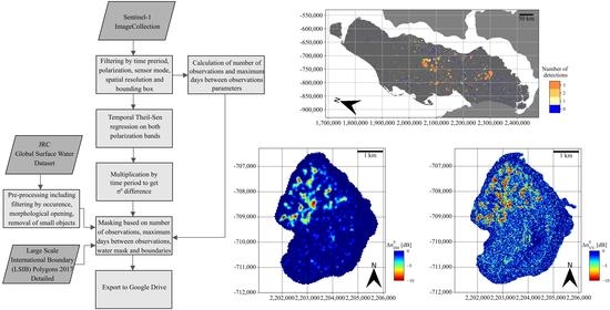
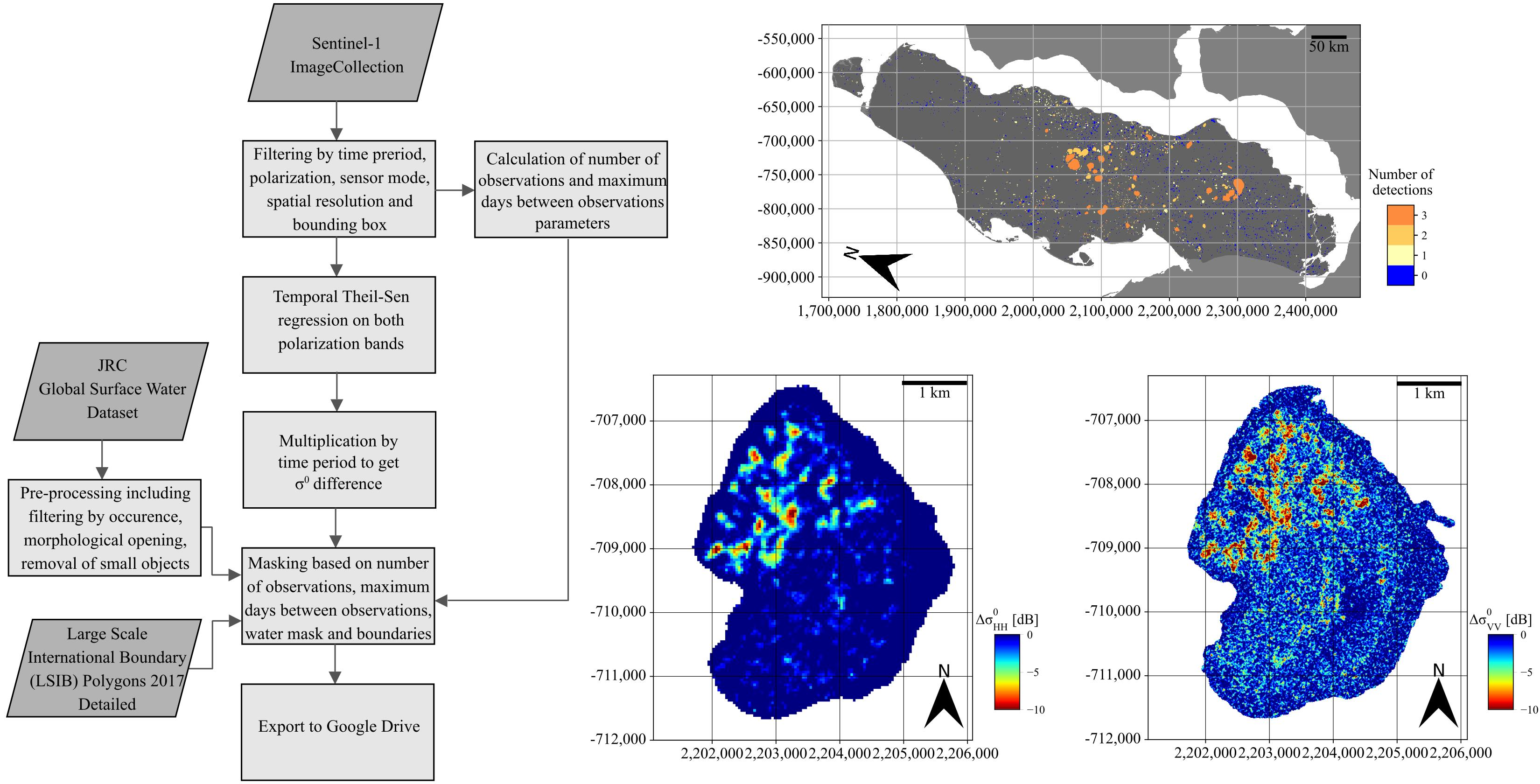
It has been shown that most backscatter anomalies on Lake Neyto first occur in late winter and spring and expand spatially over time in the years concerned [27]. We therefore sought a robust approach to characterize changes in backscatter coefficient over time. We used a temporal Theil–Sen regression [53,54] on the Sentinel-1 image collections, which was implemented on GEE through the ee.Reducer.sensSlope() method. With this method, the slope was calculated as the median of the slopes of all lines through pairs of data points. We applied this regression to both polarization channels (HH and HV in the case of EW mode; VV and VH in the case of IW mode data) independently. The lengths of the used observation periods vary between years and study sites (see Table 1). We therefore multiplied the slope output of the Theil–Sen regression by the length of the observation period to get estimates of changes in backscattering coefficient . For masking the lakes, we used the JRC GSW product. The lake mask was defined where water was detected in the majority of observations used for calculating the JRC GSW dataset (occurrence greater than 50%). In order to be able to conduct analyses on a lake object basis, the connections of river pixels to lake pixels had to be removed. We therefore used a morphological opening operation with a circular kernel and a radius of five pixels, which was implemented on GEE using the focal_min() and focal_max methods on the binary JRC GSW mask. focal_min() replaces each pixel value of the lake mask with the minimum of its neighbors defined by the kernel; focal_max() achieves the opposite. Hence, these operations can be used to remove river connections that are usually only a few pixels wide from the binary mask. A significant number of pixels should be present for each lake object in order to detect potential anomalies, and thus a minimum object size was defined using the connectedPixelCount() method on GEE. For the definition of the minimum number of connected pixels that should be retained, we considered a water body raster product of comparable resolution. The Advanced Spaceborne Thermal Emission and Reflection Radiometer (ASTER) Global Water Bodies Database (ASTWBD) product [55] contains a global coverage of water bodies larger than 0.2 km2 at a spatial resolution of approximately 30 m. Taking the differences in spatial resolution into account (30 m for ASTWBD, 40 m for Sentinel-1 EW, 10 m for Sentinel-1 IW), lake objects smaller than 222 pixels were removed (200,000 m2/302 m2 = 222). The resulting images were clipped using the LSIB dataset and the same masking as for the coverage maps using the minimum number of observations, and the maximum allowed number of days between observations was applied (see the previous section). Afterwards, the images were exported to Google Drive for further analyses on a local computer. A simplified flowchart describing the processing on GEE is shown in Figure 3.
4.2. Classification of Backscatter Anomalies on Lake Neyto, Yamal, Russia in 2016
A simple test was conducted on a local computer to see whether similar results as the classification of backscatter anomalies on Lake Neyto in [27] could be achieved on the image generated from the 2016 Sentinel-1 EW regression analysis for Lake Neyto in this study. A single Sentinel-1 EW acquisition from 16 May 2016 and a variety of image processing techniques to mask and classify the anomalies were used in [27]. Here, we used a threshold of −4 dB on both channels ( and ) and a logical OR on the binary classifications resulting from the threshold on the two channels. The threshold was defined by visual assessment. The classification was then quantitatively and visually compared to the one in [27]. Further, the locations of 718 holes in lake ice from a WorldView-2 acquisition of 22 May 2016 in [27] were also compared to the resulting classification in this study.
4.3. Object-Based Identification of Lakes with Potential Backscatter Anomalies
On a local computer, we used the Python packages of the Geospatial Data Abstraction Library (GDAL) version 3.1.4 [56], numpy version 1.19.4 [57], scikit-image (skimage) version 0.17.2 [58] and geopandas version 0.8.1 [59] for the identification of potential anomalies on single lake objects. Here, we used a more conservative approach than the one described in the previous section. Thresholds were defined as the minimum value identified by the Yen-threshold method [60] on the Sentinel-1 EW regression results of all years 2015 to 2020 on Lake Neyto (−4.04 dB in case of , −4.97 in case of ). The Yen threshold algorithm implements thresholding based on a maximum correlation criterion and is more computationally efficient than entropy measures that are similarly used for automatic thresholding. Yen-thresholding has been shown to be applicable to effectively distinguishing between anomalies and regular floating lake ice from single Sentinel-1 acquisitions and is thus expected to be also applicable here. The thresholds identified here are considered conservative since anomalies on Lake Neyto show a particularly high contrast to surrounding regular floating lake ice pixels when compared to other lakes [28]. A logical AND was used on the two outcomes to keep only pixels that were identified as potential anomalies in both channels. Connected components smaller than five pixels were removed from the classification. This conservative approach was chosen due to the lack of validation data and to potentially mitigate effects of late grounding. A shapefile containing single lake objects was produced for each year and study region, and lake polygons where potential anomalies were identified according to the method described above were assigned an attribute value of one. In order to assess the occurrence of anomalies in multiple years, a spatial join (sjoin() method in geopandas) was used to identify the number of years in which potential anomalies were mapped for each lake if the study region concerned was fully covered in more than one year. With the spatial join, the attribute values from different years were joined for each lake object based on spatial intersection, and these values were afterwards summed to get the number of years in which potential anomalies have been detected. Only years for which a full coverage of the study region was achieved were considered for consistency. Three years of full coverage were available for Yamal, and four years of full coverage for the Lena Delta. For Tazovskiy and the NPRA, only one year with full coverage was achieved. Remaining river and ocean fragments were removed manually from the resultant dataset. From these cleaned final shapefiles, the total number of lake objects considered in this study was estimated. In total, 10,838 lake objects were considered (3760 for Yamal, 3016 for Tazovskiy, 3165 for the NPRA and 897 for the Lena Delta).
5. Results
5.1. Coverage Maps
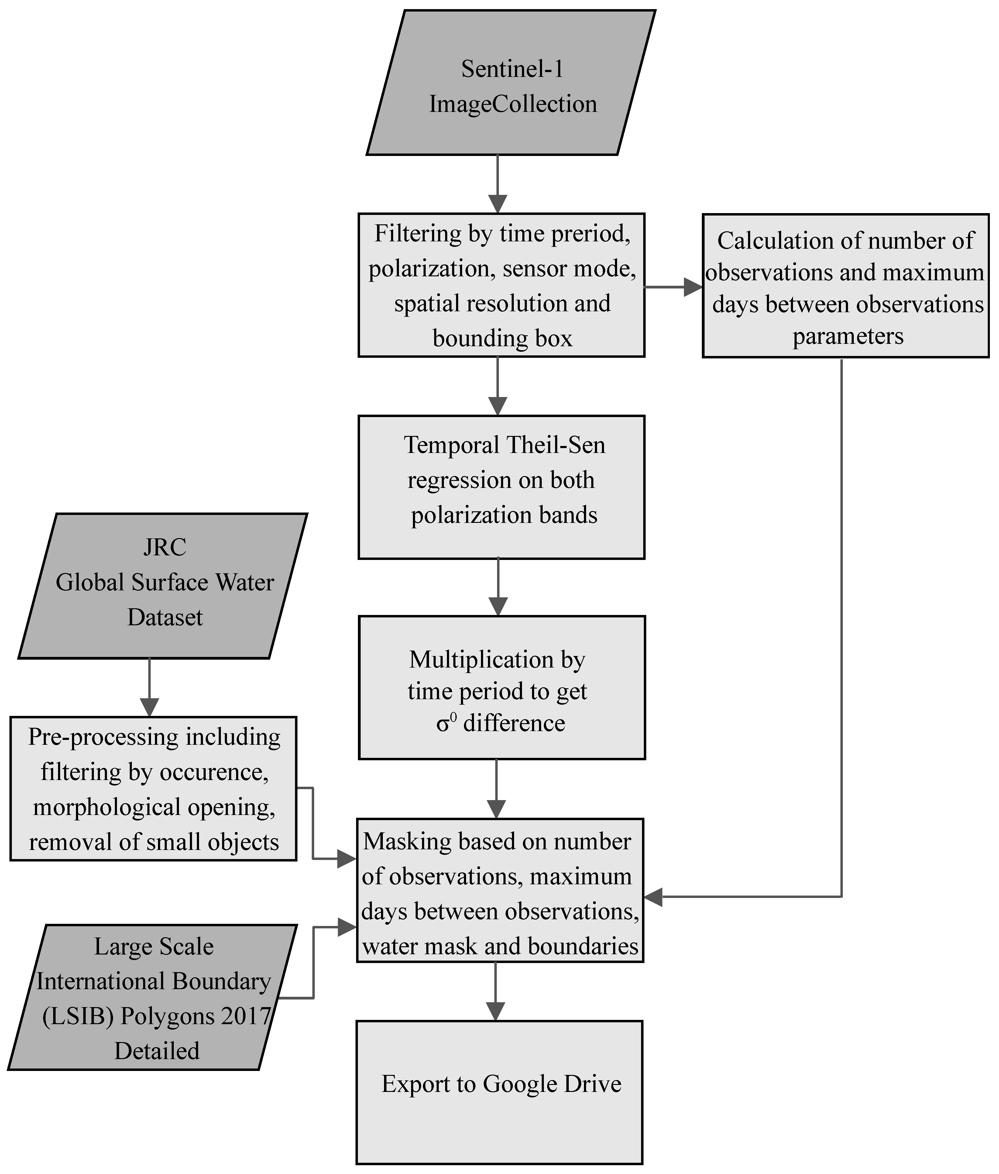
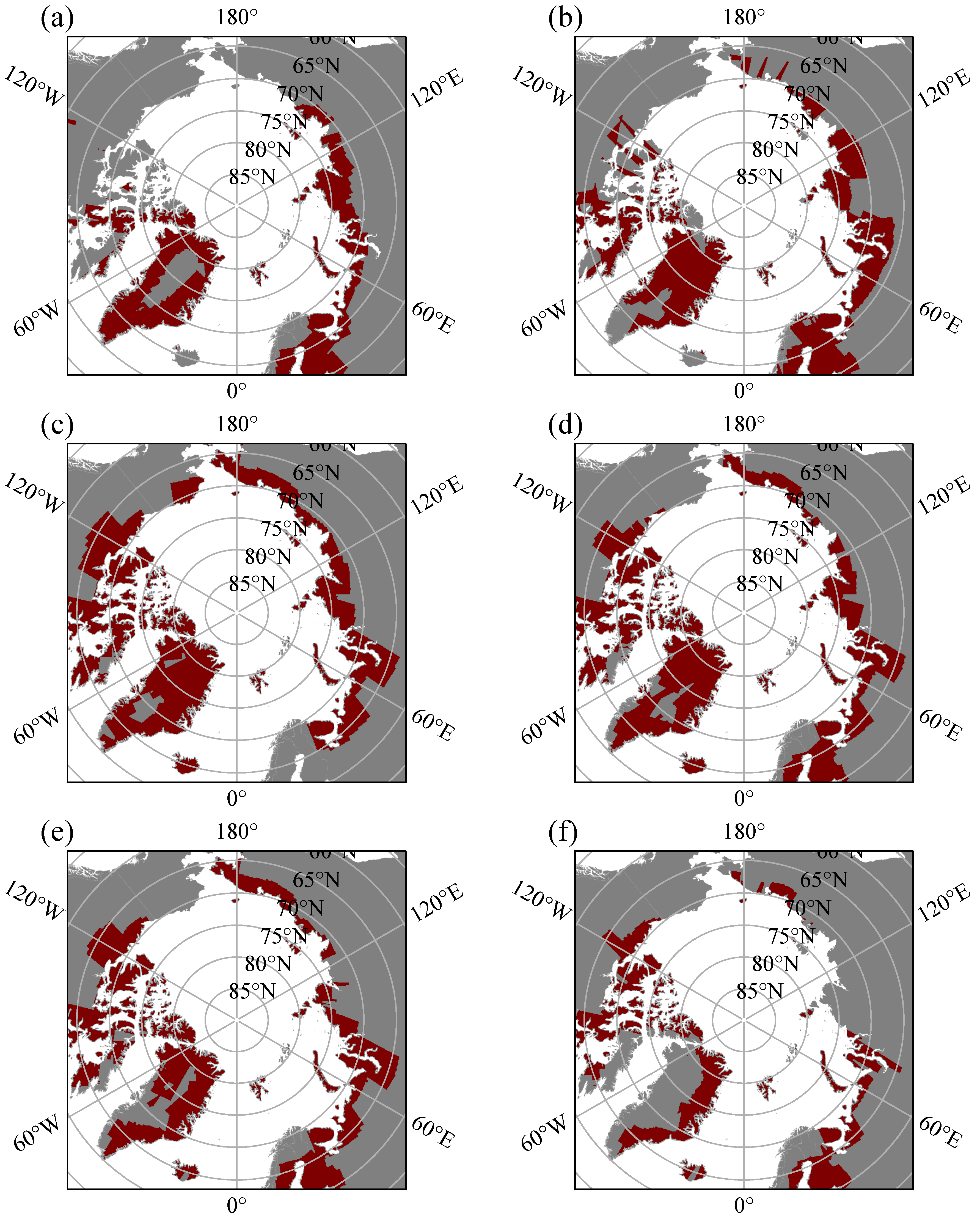
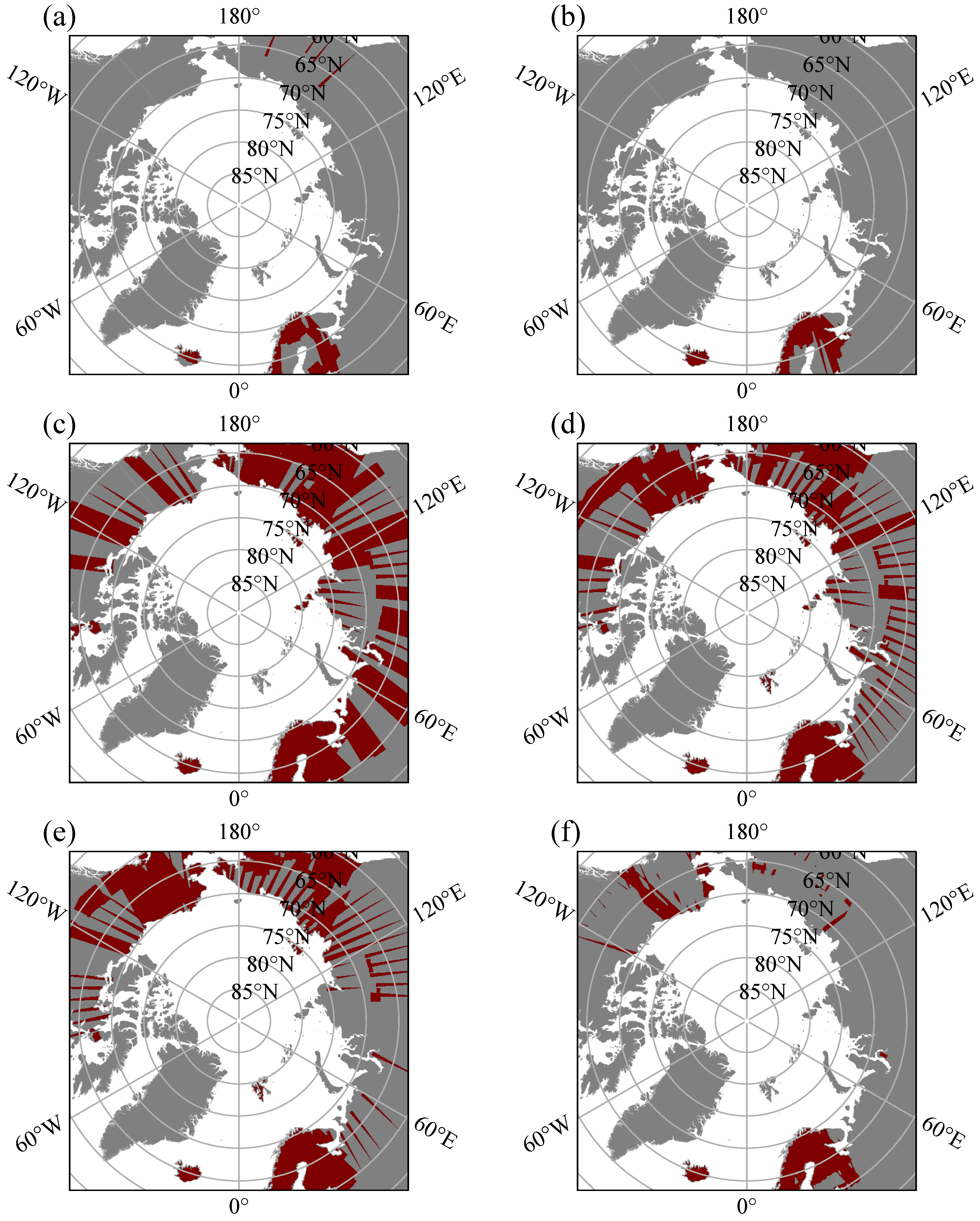
Examples of coverage maps based on the chosen parameters for the minimum number of observations (5), the maximum days allowed between observations (12), start date 1 April and the end dates (melt-onset) as identified for the Yamal Peninsula (Table 1) are shown in Figure 4 for EW mode with HH and HV polarization, and in Figure 5 for IW mode with VV and VH polarization. The panels (a) to (f) indicate the analyzed years 2015 to 2020, respectively. In addition to the maps presented here, coverage maps were calculated for all time periods considered in this study (see the supplement to this article [51]), and similar patterns could be identified as for the examples in Figure 4 and Figure 5. Covered regions vary significantly between years. IW coverage extends further south, but in many cases, only narrow stripes of coverage are apparent. No IW coverage of any parts of our study regions was achieved in 2015 or 2016. Higher coverage of our study sites in EW mode in general is apparent.
5.2. Lake Neyto and Comparison to Previous Study
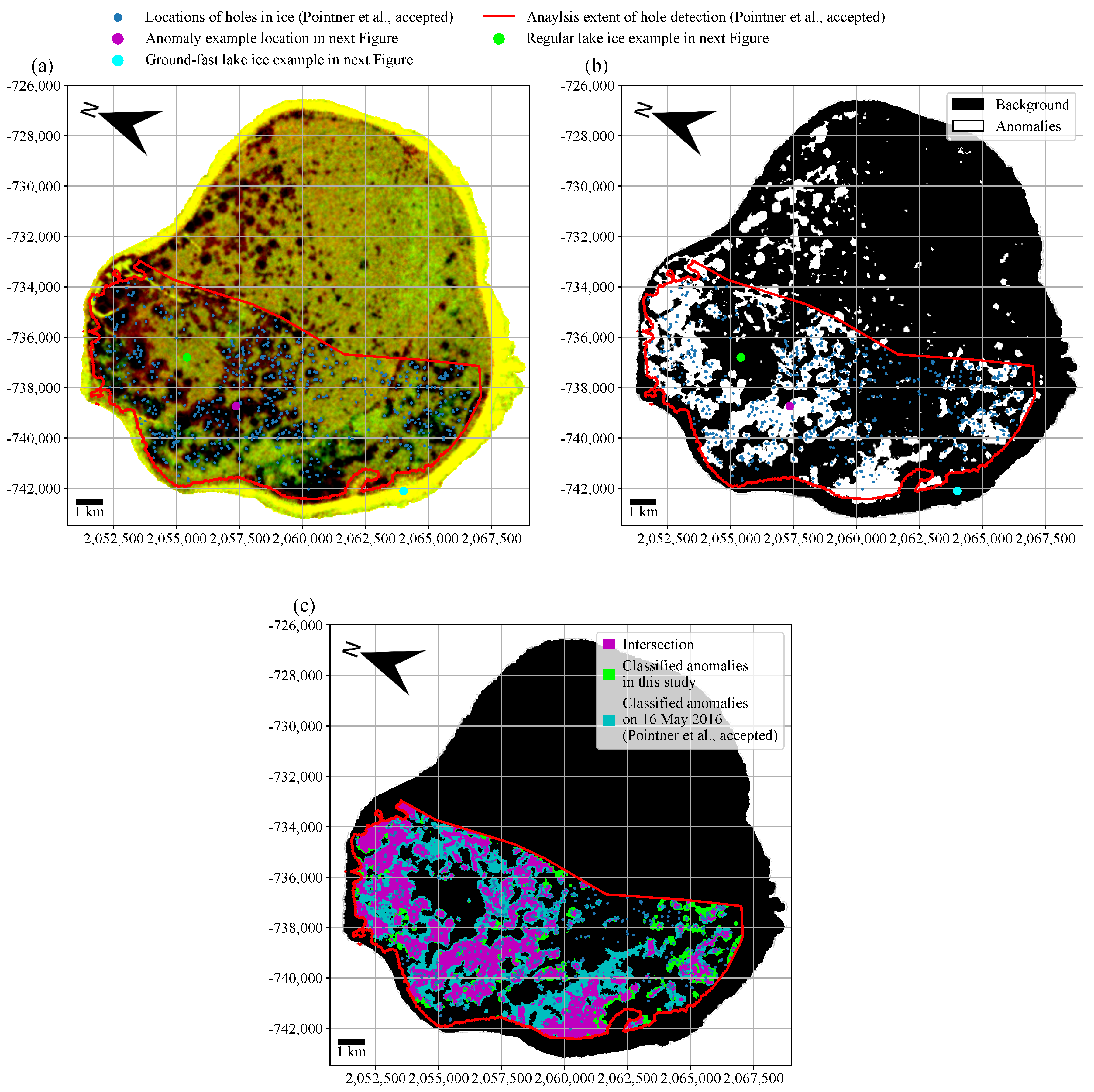
Visualizations of results for Lake Neyto, where characteristic anomalies were first identified and described [14], are depicted in Figure 6 for the year 2016 with start date 1 March. A color composite (red channel: , green channel: , blue channel: constant 0, scaling for and between −5 and 5 dB) is shown in Figure 6a. The classification result from thresholding (−4 dB threshold) and subsequent logical OR on the two bands is shown in Figure 6b. Figure 6c indicates a comparison between the classification in this study (Figure 6b) and the one in [27], showing intersecting areas and areas that were only classified in one of the two studies. Locations of mapped holes in the lake ice from VHR optical data from 22 May 2016 (blue dots [27]) are shown in all panels (a)–(c). The analysis extent for the mapping of the holes and comparison to SAR classification results in [27] (red outline) is indicated in all panels (a)–(c) as well. For the comparison to results in [27], this analysis extent was considered. Example locations of a point considered regular floating lake ice (green dot), a point considered ground-fast lake ice (cyan dot) and a hole identified in [27] (magenta dot) are shown in panels (a) and (b) and were used for showing time series examples in the following Figure 7. Seventy-five percent of the holes lay within the classified regions shown in Figure 6b. In comparison, 71% of the holes lay in the classified regions of [27].
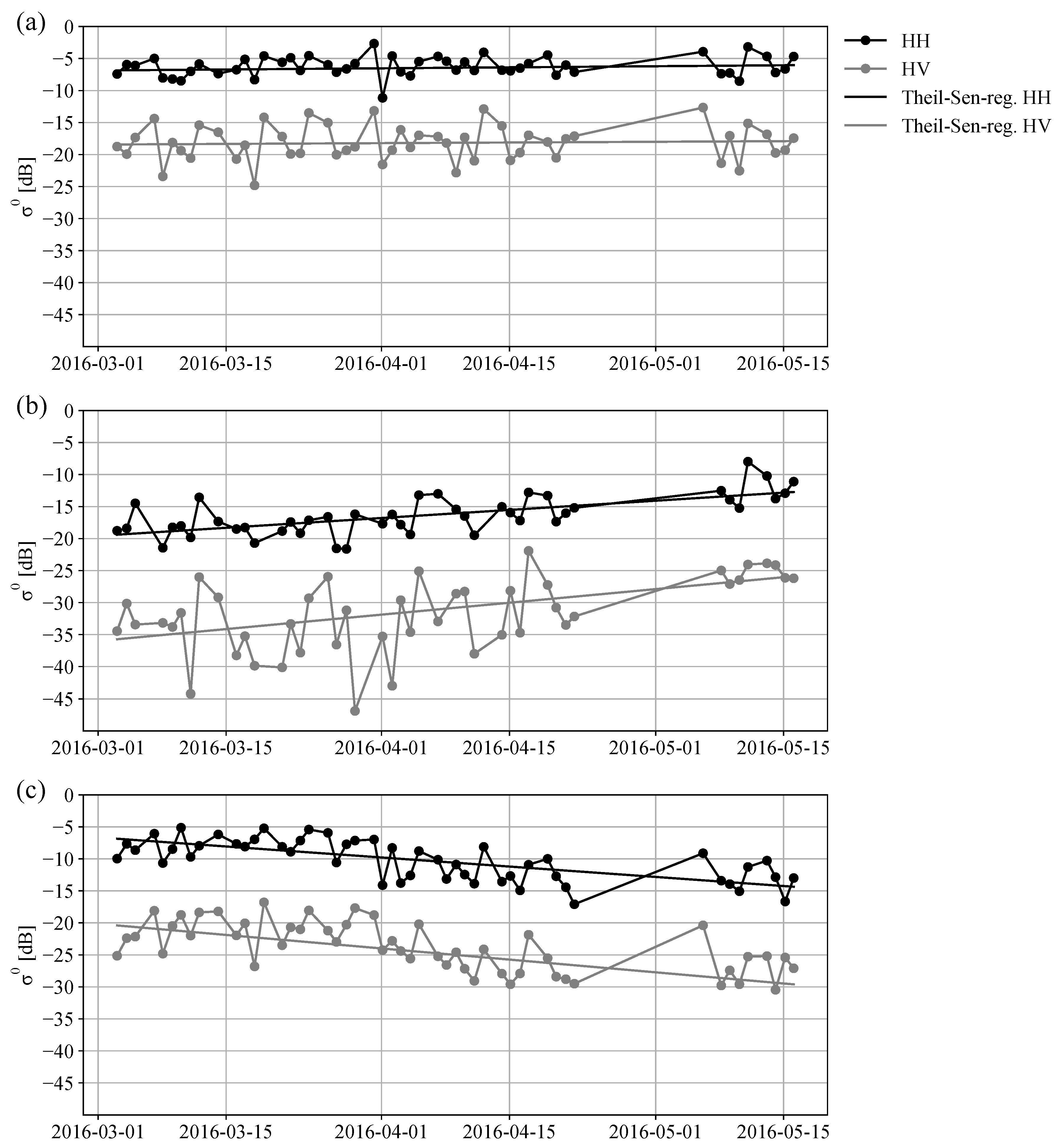
Figure 7a shows time series for the green dot (regular floating lake ice) in Figure 6, Figure 7b shows time series for the cyan dot (ground-fast lake ice) in Figure 6 and Figure 7c shows time series for the magenta dot (backscatter anomalies) in Figure 6. HH and HV-channel data and associated temporal Theil–Sen regression lines are depicted. The slopes are similar among the polarization channels in all panels (a), (b) and (c). The slope of for the regular floating lake ice location is close to zero, while a clear change in backscatter is indicated by the slope of for the anomaly location. Similar values for at the beginning of the time series can be identified when comparing Figure 7a,c. The slope of the example for ground-fast lake ice in Figure 7b indicates a significant increase of backscatter over time, but such an increase was only observed in 2016 and was potentially related to the period of melt that also led to the exclusion of several acquisitions (the backscatter after the gap in the time series in Figure 7b is higher than before). In other years, slopes similar to floating lake ice were observed [51].
5.3. Lake Object-Based Counts of Years with Potential Anomalies Detected
Lake object-based detection of potential anomalies was performed for each year separately, and the number of years with detections was identified for each lake over all years where the entire study region was covered for consistency (see Section 4.3). Hence, the number of years that could be considered varies between study regions. For Yamal, the years 2017, 2018 and 2019 could be used. For the Lena Delta, the years 2015, 2016, 2017 and 2018 could be used. Only a single year of entire coverage could be considered for Tazovskiy (2016) and the NPRA (2017). The results of the number of years with detection per lake are shown in Figure 8. Strong differences between study regions can be observed: on Yamal (Figure 8a) relatively many lakes with potential anomalies detected in multiple years were found. The number of classes in Figure 8a–d reflects the number of years that could be considered.
Percentages of lakes where potential anomalies were detected in a specific number of years with respect to the total number of lakes are shown in Table 2 for all study regions. For Tazovskiy and the NPRA, where only one year could be considered, 8% and 4% of lakes with anomalies were identified, respectively. For the Lena Delta (4 years considered), for 13% and 2% of lakes, potential anomalies were detected in 1 and 2 years, respectively, but no lakes were identified where potential anomalies were detected in 3 or 4 years. For Yamal, for more than 30% of lakes potential anomalies were detected in at least 1 of 3 years.
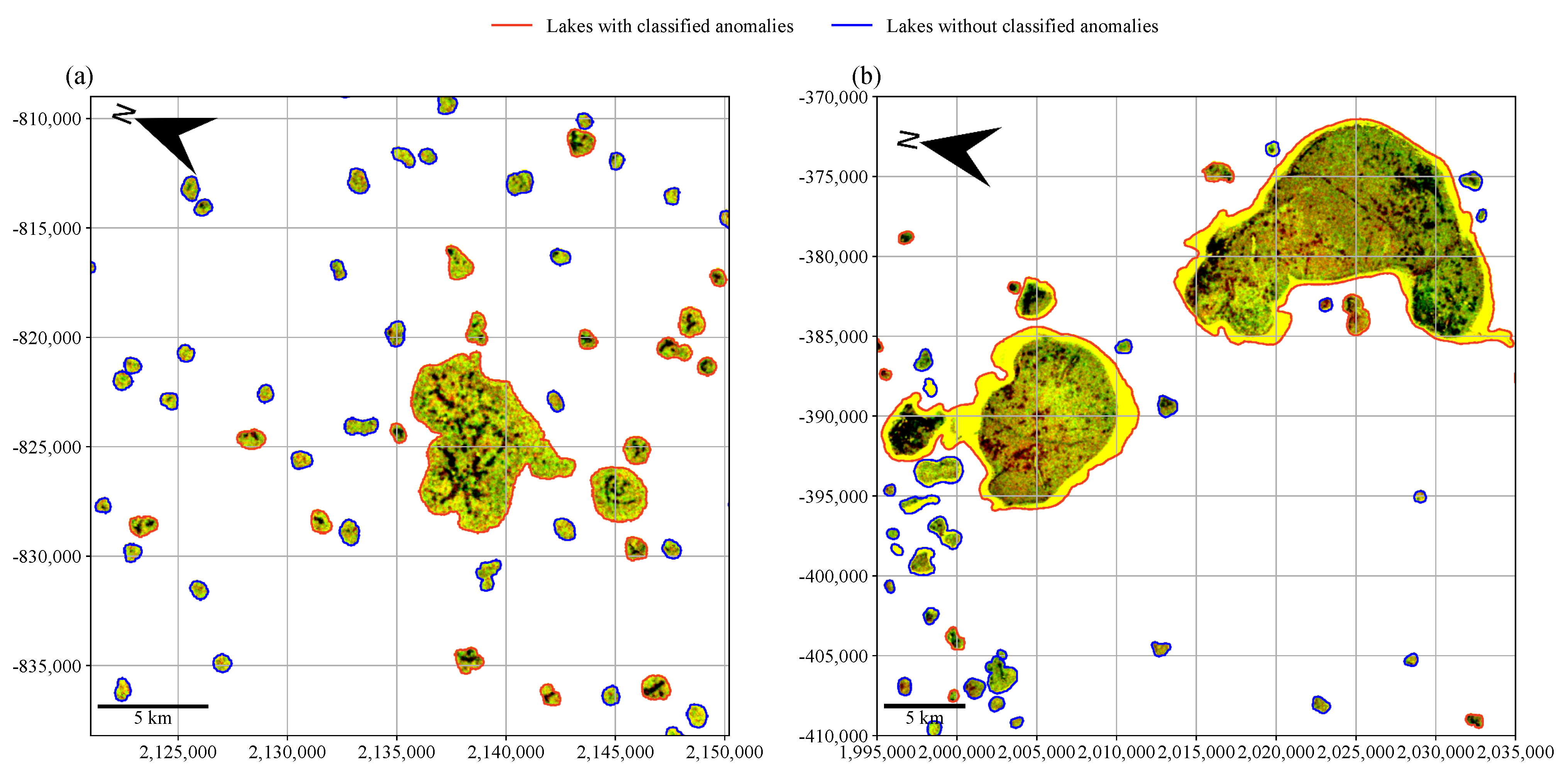
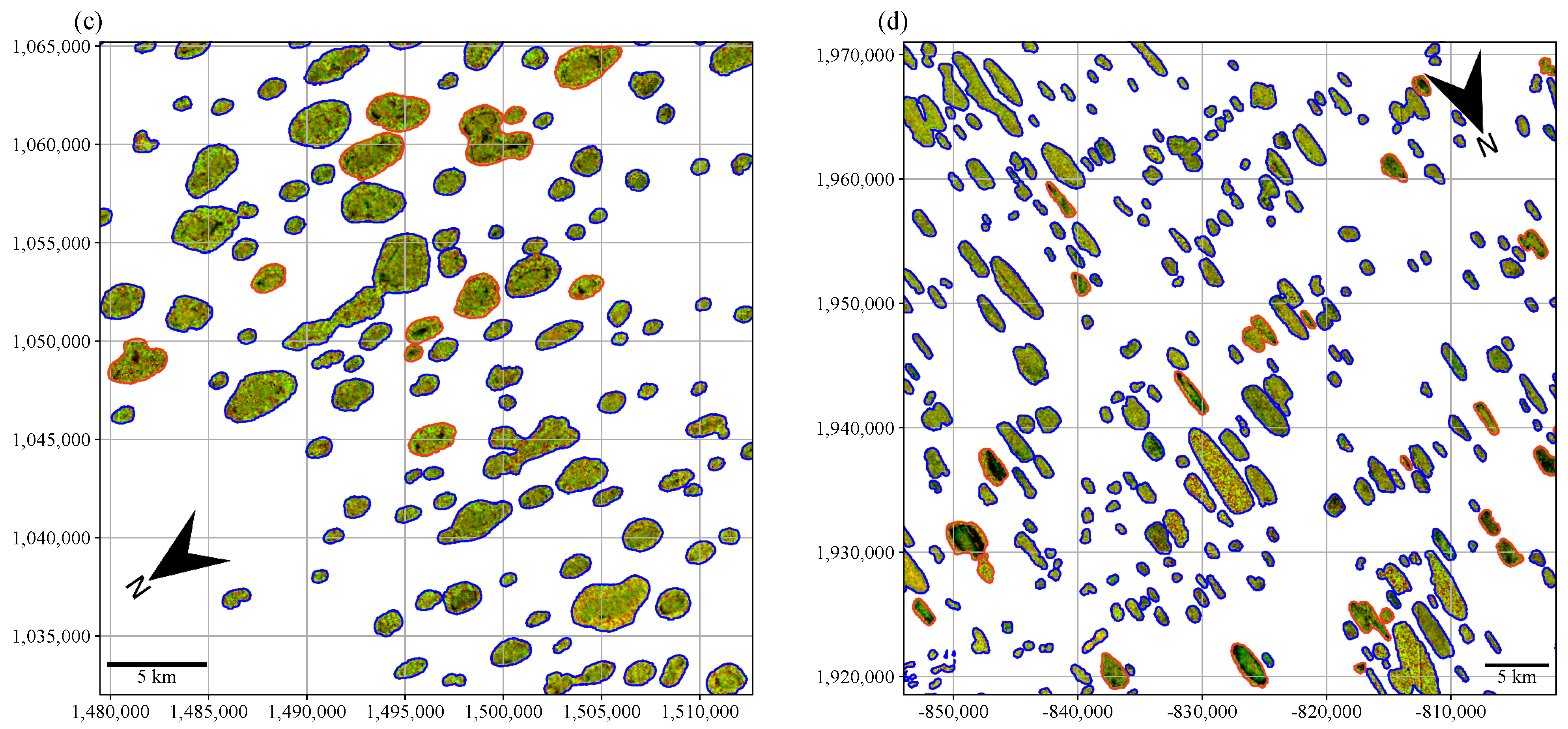
A notable number of lakes where potential anomalies were detected in at least one year was identified for every study region. However, upon visual inspections of the produced datasets [51], strong differences in the visual appearance of potential anomalies were encountered between regions. Examples of sub-regions for each study site in years considered for object-based detection of potential anomalies (Figure 8 and Table 2) are depicted in Figure 9. Classification as a lake with potential anomalies is indicated by the color of the outline (red for potential anomalies identified, blue for no potential anomalies identified). Anomalies that clearly resemble the anomalies on Lake Neyto were visually only identified in regions on the Yamal and Tazovskiy Peninsulas.
5.4. Visualizations of Co-Polarized -Images
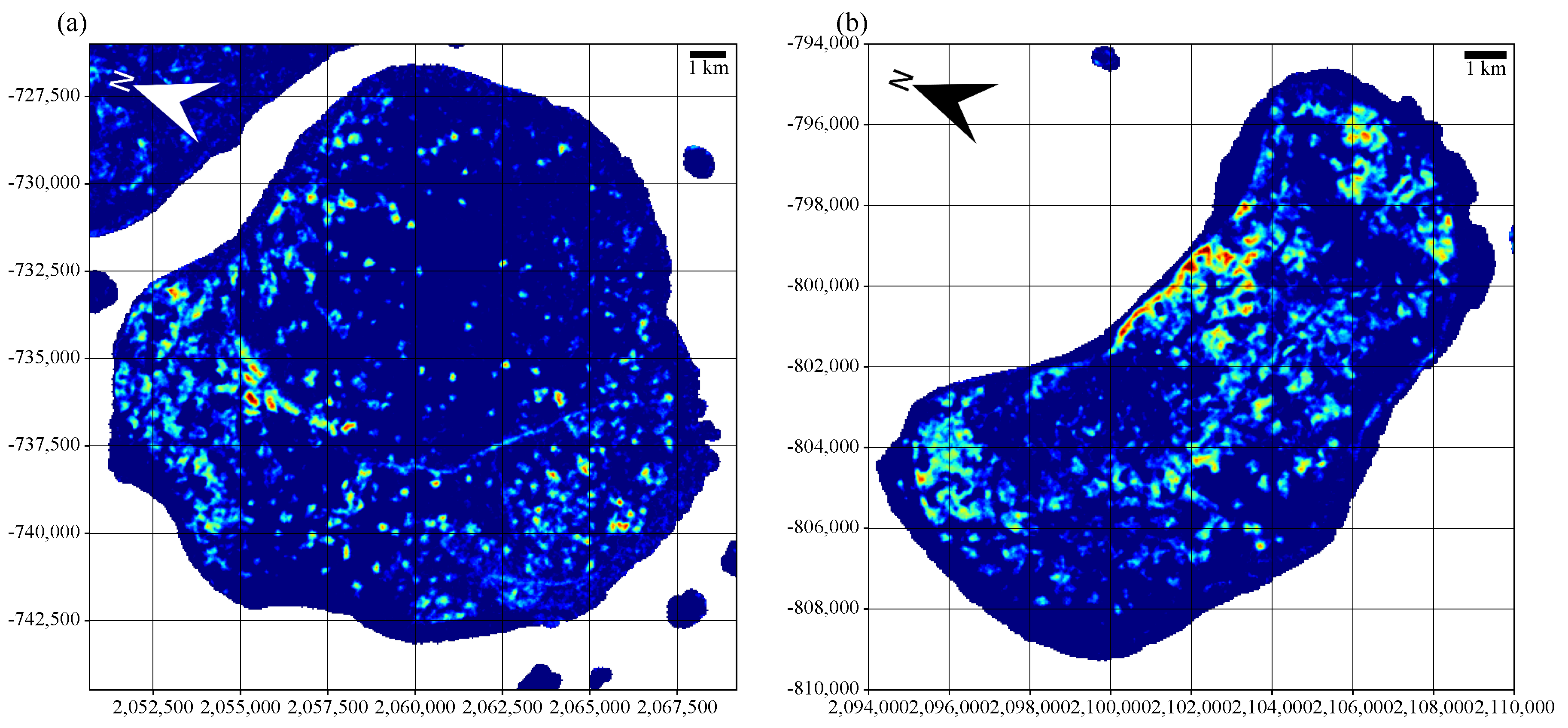
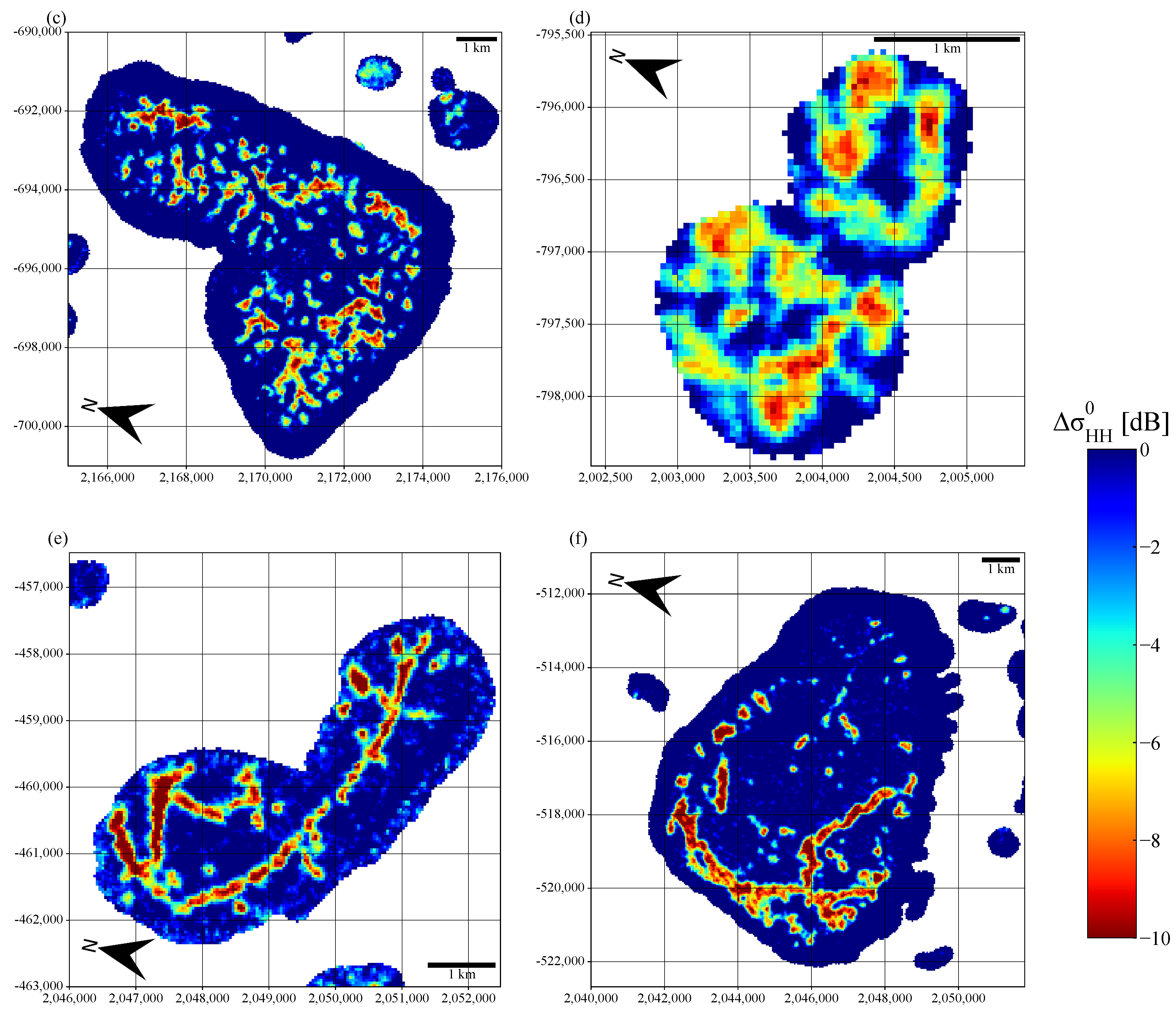
In Figure 10, visualizations of -images for Lake Neyto (Figure 10a) and lakes on Yamal and Tazovskiy with similar anomalies (Figure 10b–f) can be seen. Smaller round and larger more elongated objects are often apparent. A striking characteristic of most groups of backscatter anomaly pixels is a significant gradient from the center to the outer parts.
Where spatio-temporal data coverage allows it, results of time series analyses can be directly compared between EW mode and IW mode. A comparison between a image from EW mode and a image form IW mode for a lake on the Yamal Peninsula with start date 1 March in 2019 is presented in Figure 11. While the in Figure 11b appears noisier than the in Figure 11a, strong spatial similarities can nevertheless be identified.
6. Discussion
The spatio-temporal data distribution is important for the interpretation of big Earth data time series analyses [61]. Apart from the definitions of start and end dates, as discussed in Section 3.1, we used the minimum number of observations and maximum allowed days between observation parameters to constrain our analyses to areas and time periods with meaningful data distributions. The algorithm [51], which takes these parameters into account, could also be useful for other time series-based studies on GEE in the future and is not limited to Sentinel-1 SAR data.
Irregularities in coverage between the years can be identified for both modes (Figure 4 and Figure 5), but are more pronounced in IW mode, where in 2015 and 2016 no parts of our study sites were covered. With the parameters chosen in Figure 4 and Figure 5 (start date 1 April; end dates as identified for the Yamal Peninsula in Table 1; minimum number of observations 5; maximum allowed days between observations 12), full coverage of the study regions was achieved in three years for Yamal and the Lena Delta, and one year of full coverage was achieved for the Tazovskiy Peninsula and the NPRA. On the other hand, with IW mode, the Yamal, Tazovskiy and NPRA study regions could not be fully covered in any of the years available. Only the Lena Delta study region was fully covered in two years in IW mode. These interpretations explain why EW data were prioritized in this study, and similar interpretations can be made when considering coverage maps for all combinations of start (1 March and 1 April) and end dates (Table 1), which are given in the supplementary material of this article [51]. However, the analyses with IW data could be useful for smaller study regions or for comparisons with the EW results, where coverage allows it.
Backscatter anomaly classifications results on Lake Neyto in 2016 are similar to the ones presented in [27] (Figure 6). Eighty-six percent of the classified area in this study intersects with the classified area in [27] (Figure 6c). However, the classified area in this study is clearly smaller (76% of the area in [27]). This could have been expected, since the very last Sentinel-1 acquisition from 16 May before melt-onset in 2016 was used in [27] for the classification. Given that anomalies expand significantly during the last useful observation dates in the season [27], the robust temporal Theil–Sen regression likely could not account for the expansion during the very last observations before melt-onset. Nevertheless, the fractions of holes found toobject-basedwithin the classified anomalies are similar (75% in this study, 71% in [27]). Potential interconnected reasons for 25% of holes not being located in delineated anomaly regions include later flooding through some holes, limited spatial resolution of the Sentinel-1 EW SAR data (40 m), variations in snow depth and the imperfectness of the classification method [27]. Of course, the selection of the −4 dB threshold for both channels and the selection of the logical OR applied in the following analysis were to some degree arbitrary, but this analysis was only intended to show that we can achieve similar results to [27] using a very simple method on the output images generated on GEE. On the contrary, a variety of pre-processing, masking and image processing steps were required to produce the classification result in [27].
The example time series in Figure 7 illustrate the usefulness of the robust Theil–Sen regression approach to account for noise and also potentially incidence angle effects. Variations of over time can be seen for the regular floating ice example in Figure 7a, but overall the backscatter seemed to remain at a similar level, which is reflected by slopes close to zero. Strong variations can also be identified for the anomaly example in Figure 7c, but roughly two different levels of backscatter in time can be made out, which is reflected by significant slopes of the associated Theil–Sen regression lines.
Automatic classification of anomalies for single lakes and counting of the number of years where anomalies were identified for each lake were attempted in this study (Figure 8 and Figure 9), and a particularly high number of lakes with anomalies in multiple years was detected on the Yamal Peninsula (Table 2). However, we identified a number of issues related to this approach that need to be discussed. Potential anomalies identified in the Lena Delta and the NPRA (Figure 8c,d, respectively) do not resemble characteristic anomalies on Lake Neyto and are most likely induced by late grounding of the ice. A similar drop in backscatter as for the anomalies was observed in the case of grounding (see Section 3.1). Many Arctic lakes are characterized by shallow shelf zones, of which the boundary to a central deeper part is more or less parallel to the lake outline [33] (see Figure 2). Many pixels of low in Figure 9c,d that can occur along these boundaries are thus likely artifacts caused by late grounding. Here, 1 April was chosen as the start date as a trade-off between artifacts caused by late grounding and temporal data coverage. However, the results show that conceivable effects of late grounding may occur, as ice can thicken in late winter and spring until melt-onset. Such effects can never be ruled out and may therefore also be present in the other two study regions, so the results presented in Figure 8 and Table 2 should be treated extremely carefully. Another mechanism that could lead to a significant drop in backscatter and therefore affect automatic classification might be cracking and subsequent flooding of the ice layer [18]. Other, yet unknown factors may also lead to similar anomalies, but in the absence of further reference data, we could not deduce how many anomalies might potentially be related to methane emissions and how many to other factors. Upon the clarification of the mechanism that leads to the observed anomalies on Lake Neyto, a more sophisticated approach to mapping similar anomalies on other lakes might therefore be beneficial in future studies, but the need for an additional visual interpretation will likely remain. In addition, a less arbitrary approach to define the start dates might be desirable, but in the absence of a deeper understanding of the driving factors leading to the emergence of anomalies, this was not further assessed.
For the selection of target areas for future field-based and remote sensing studies, visualizations of the results may be sufficient or even more important than the automatic classification of the images. The best candidates for lakes with similar mechanisms leading to anomalies as on Lake Neyto seem to be identifiable through characteristic shapes of anomalies in the visualizations of images. Patterns that clearly resemble observed anomalies on Lake Neyto (combination of round and elongated objects) were identified visually only on lakes on the Yamal and Tazovskiy Peninsulas (Figure 9a,b, Figure 10 and Figure 11). We strongly encourage the reader to visualize the results given in the Supplementary Information in order to clearly comprehend these interpretations. Interestingly, the visualizations of the images seem to reflect the expansion of the anomalies. Anomaly regions on Lake Neyto are expanding over time [27], which seems to be reflected by a gradient in the image from the center to the outer parts of cluster of anomalies in Figure 10a, and similar effects can be seen in the examples for the other lakes in Figure 10b–f. Exploiting this effect might help to constrain potential target areas for field-based research to a few Sentinel-1 EW pixels.
The identified coverage for the higher-resolution IW data (Figure 5) is limited, but where available, results from IW mode can be used for a comparison to the EW mode results (Figure 11). Although the image in Figure 11b appears noisier than the image in Figure 11a, similar structures can be identified easily. Regions that appear similar in the two modes might be prioritized in the selection of field sites in future research.
7. Conclusions
In this study, we provided the first regional accounts for lake ice C-band SAR backscatter anomalies (pixels that turn from relatively high backscatter to relatively low backscatter over time in late winter and spring) using a time series analysis-based algorithm on Sentinel-1 data on Google Earth Engine (GEE). Previous studies have suggested a potential connection between anomalies and methane emissions. Hence, the results produced in this study are expected to be useful for identifying target areas for future field research in different regions and possibly for understanding the abundance of lake methane seeps upon the clarification of the mechanisms involved. Coverage maps were produced taking the number of observations and days between observations into account. The algorithm for deriving these maps is independent of the sensor and could thus be useful for a variety of future studies on GEE. Coverage varies between years for both EW and IW modes of Sentinel-1, but better overall coverage of our four study regions was achieved in EW mode. However, results from IW mode could be useful for smaller study regions and for a comparison to the EW results, where both are available. For Lake Neyto on the Yamal Peninsula, where anomalies have been first described and quantified, a simple threshold-based classification on images produced on GEE showed good agreement with the classification from a previous study, and the locations of three quarters of the holes identified in the lake ice were found to be related to the anomalies classified in this study. Automatic threshold-based identification of anomalies from the images and counting of years where anomalies have been identified were attempted for each lake in the study regions, but some issues were identified. Most importantly, the ice may still thicken during the analysis periods, and hence manifestations of late grounding of the ice and anomalies could not be separated effectively. Thus, the associated results should be treated very carefully and a more sophisticated method to classify anomalies similar to those on Lake Neyto might be beneficial upon the clarification of the associated mechanisms for future studies, but the need for additional visual interpretation is expected to remain. General limitations of our study are that the connection between anomalies and methane emissions on Lake Neyto has not been verified with in-situ data and the obvious lack of further reference data, preventing a more detailed analysis of the driving factors leading to the observed anomalies on regional scales. The largest benefit of this work is expected to arise from visualizations of the resulting images for the selection of target areas for future field research. Visualizations seem to be capable of reflecting the expansion of anomaly regions over time. Where available, comparisons between results from EW and IW mode could further aid this selection. Anomalies that clearly resemble those on Lake Neyto in terms of shape were identified solely visually for lakes on the Yamal and Tazovskiy Peninsulas. The datasets and Python code for reproducing the results are available from Zenodo in the Supplementary Materials. The algorithm can be easily adapted to other study regions and future years.
Author Contributions
Conceptualization, G.P. and A.B.; methodology, G.P.; software, G.P.; validation, G.P.; formal analysis, G.P.; investigation, G.P.; resources, A.B.; data curation, G.P.; writing—original draft preparation, G.P. and A.B.; writing—review and editing, G.P. and A.B.; visualization, G.P.; supervision, A.B.; project administration, A.B.; funding acquisition, A.B. All authors have read and agreed to the published version of the manuscript.
Funding
This work was supported by the European Union’s HORIZON2020 research projects Nunataryuk (grant number 773421) and CHARTER (grant number 869471), and the doctoral college DK GIScience at the University of Salzburg (Austrian Science Fund (FWF) project number W 1237).
Institutional Review Board Statement
Not applicable.
Informed Consent Statement
Not applicable.
Data Availability Statement
Geospatial data (images and vector data) produced in this study and Python code to reproduce the results are openly shared from Zenodo at doi:10.5281/zenodo.4694533, reference number [51]. In order to retain the directory structure, which is essential for the comprehensibility, the files had to be uploaded as single zip archive. Two reduced versions of the dataset with smaller overall file size are thus also provided. Please see the Zenodo record for details. If download problems are encountered or single files are needed, data can also be provided by contacting the corresponding author.
Acknowledgments
Contains modified Copernicus Sentinel data (2015–2020). Data provided by the European Space Agency. WorldView-2 data © DigitalGlobe, Inc. (2016), provided by European Space Imaging through the European Space Agency (ESA) third party mission program (Project ID 54392).
Conflicts of Interest
The authors declare no conflict of interest. The funders had no role in the design of the study; in the collection, analyses, or interpretation of data; in the writing of the manuscript, or in the decision to publish the results.
References
- Bartsch, A.; Pointner, G.; Leibman, M.O.; Dvornikov, Y.A.; Khomutov, A.V.; Trofaier, A.M. Circumpolar Mapping of Ground-Fast Lake Ice. Front. Earth Sci. 2017, 5, 12. [Google Scholar] [CrossRef] [Green Version]
- Walter Anthony, K.M.; Anthony, P.; Grosse, G.; Chanton, J. Geologic methane seeps along boundaries of Arctic permafrost thaw and melting glaciers. Nat. Geosci. 2012, 5, 419–426. [Google Scholar] [CrossRef]
- Wik, M.; Varner, R.K.; Anthony, K.W.; MacIntyre, S.; Bastviken, D. Climate-sensitive northern lakes and ponds are critical components of methane release. Nat. Geosci. 2016, 9, 99–105. [Google Scholar] [CrossRef]
- Bastviken, D.; Tranvik, L.J.; Downing, J.A.; Crill, P.M.; Enrich-Prast, A. Freshwater Methane Emissions Offset the Continental Carbon Sink. Science 2011, 331, 50. [Google Scholar] [CrossRef] [PubMed] [Green Version]
- Bastviken, D.; Cole, J.; Pace, M.; Tranvik, L. Methane emissions from lakes: Dependence of lake characteristics, two regional assessments, and a global estimate. Glob. Biogeochem. Cycles 2004, 18. [Google Scholar] [CrossRef]
- Walter, K.M.; Smith, L.C.; Stuart Chapin, F., III. Methane bubbling from northern lakes: Present and future contributions to the global methane budget. Philos. Trans. R. Soc. Math. Phys. Eng. Sci. 2007, 365, 1657–1676. [Google Scholar] [CrossRef] [PubMed]
- Walter, K.M.; Engram, M.; Duguay, C.R.; Jeffries, M.O.; Chapin, F. The Potential Use of Synthetic Aperture Radar for Estimating Methane Ebullition From Arctic Lakes. JAWRA J. Am. Water Resour. Assoc. 2008, 44, 305–315. [Google Scholar] [CrossRef]
- Anthony, K.W.; Daanen, R.; Anthony, P.; von Deimling, T.S.; Ping, C.L.; Chanton, J.P.; Grosse, G. Methane emissions proportional to permafrost carbon thawed in Arctic lakes since the 1950s. Nat. Geosci. 2016, 9, 679–682. [Google Scholar] [CrossRef]
- Wik, M.; Crill, P.M.; Bastviken, D.; Danielsson, Å.; Norbäck, E. Bubbles trapped in arctic lake ice: Potential implications for methane emissions. J. Geophys. Res. Biogeosci. 2011, 116. [Google Scholar] [CrossRef] [Green Version]
- Engram, M.; Walter Anthony, K.; Meyer, F.J.; Grosse, G. Synthetic aperture radar (SAR) backscatter response from methane ebullition bubbles trapped by thermokarst lake ice. Can. J. Remote Sens. 2013, 38, 667–682. [Google Scholar] [CrossRef]
- Engram, M.; Walter Anthony, K.; Sachs, T.; Kohnert, K.; Serafimovich, A.; Grosse, G.; Meyer, F. Remote sensing northern lake methane ebullition. Nat. Clim. Chang. 2020, 10, 511–517. [Google Scholar] [CrossRef]
- Turetsky, M.R.; Abbott, B.W.; Jones, M.C.; Anthony, K.W.; Olefeldt, D.; Schuur, E.A.; Grosse, G.; Kuhry, P.; Hugelius, G.; Koven, C.; et al. Carbon release through abrupt permafrost thaw. Nat. Geosci. 2020, 13, 138–143. [Google Scholar] [CrossRef]
- Bogoyavlensky, V.I.; Sizov, O.S.; Bogoyavlensky, I.V.; Nikonov, R.A. Remote identification of areas of surface gas and gas emissions in the Arctic: Yamal Peninsula. Arct. Ecol. Econ. 2016, 3, 4–15. (in Russian). [Google Scholar]
- Bogoyavlensky, V.I.; Sizov, O.S.; Bogoyavlensky, I.V.; Nikonov, R.A. Technologies for Remote Detection and Monitoring of the Earth Degassing in the Arctic: Yamal Peninsula, Neito Lake. Arct. Ecol. Econ. 2018, 2, 83–93. (in Russian). [Google Scholar] [CrossRef]
- Bogoyavlensky, V.I.; Bogoyavlensky, I.V.; Kargina, T.N.; Nikonov, R.A.; Sizov, O.S. Earth degassing in the Artic: Remote and field studies of the thermokarst lakes gas eruption. Arct. Ecol. Econ. 2019, 2, 31–47. (in Russian). [Google Scholar] [CrossRef]
- Chuvilin, E.; Ekimova, V.; Davletshina, D.; Sokolova, N.; Bukhanov, B. Evidence of Gas Emissions from Permafrost in the Russian Arctic. Geosciences 2020, 10, 383. [Google Scholar] [CrossRef]
- Surdu, C.M.; Duguay, C.R.; Pour, H.K.; Brown, L.C. Ice Freeze-up and Break-up Detection of Shallow Lakes in Northern Alaska with Spaceborne SAR. Remote Sens. 2015, 7, 6133–6159. [Google Scholar] [CrossRef] [Green Version]
- Duguay, C.R.; Pietroniro, A. Remote Sensing in Northern Hydrology: Measuring Environmental Change. Wash. DC Am. Geophys. Union Geophys. Monogr. Ser. 2005, 163. [Google Scholar] [CrossRef]
- Antonova, S.; Duguay, C.R.; Kääb, A.; Heim, B.; Langer, M.; Westermann, S.; Boike, J. Monitoring Bedfast Ice and Ice Phenology in Lakes of the Lena River Delta Using TerraSAR-X Backscatter and Coherence Time Series. Remote Sens. 2016, 8, 903. [Google Scholar] [CrossRef] [Green Version]
- Duguay, C.R.; Lafleur, P.M. Determining depth and ice thickness of shallow sub-Arctic lakes using space-borne optical and SAR data. Int. J. Remote Sens. 2003, 24, 475–489. [Google Scholar] [CrossRef]
- Engram, M.; Arp, C.D.; Jones, B.M.; Ajadi, O.A.; Meyer, F.J. Analyzing floating and bedfast lake ice regimes across Arctic Alaska using 25 years of space-borne SAR imagery. Remote Sens. Environ. 2018, 209, 660–676. [Google Scholar] [CrossRef]
- Grunblatt, J.; Atwood, D. Mapping lakes for winter liquid water availability using SAR on the North Slope of Alaska. Int. J. Appl. Earth Obs. Geoinf. 2014, 27, 63–69. [Google Scholar] [CrossRef]
- Surdu, C.M.; Duguay, C.R.; Brown, L.C.; Fernández Prieto, D. Response of ice cover on shallow lakes of the North Slope of Alaska to contemporary climate conditions (1950–2011): Radar remote-sensing and numerical modeling data analysis. Cryosphere 2014, 8, 167–180. [Google Scholar] [CrossRef] [Green Version]
- Duguay, C.R.; Pultz, T.J.; Lafleur, P.M.; Drai, D. RADARSAT backscatter characteristics of ice growing on shallow sub-Arctic lakes, Churchill, Manitoba, Canada. Hydrol. Process. 2002, 16, 1631–1644. [Google Scholar] [CrossRef]
- Atwood, D.K.; Gunn, G.E.; Roussi, C.; Wu, J.; Duguay, C.; Sarabandi, K. Microwave Backscatter From Arctic Lake Ice and Polarimetric Implications. IEEE Trans. Geosci. Remote Sens. 2015, 53, 5972–5982. [Google Scholar] [CrossRef]
- Gunn, G.E.; Duguay, C.R.; Atwood, D.K.; King, J.; Toose, P. Observing Scattering Mechanisms of Bubbled Freshwater Lake Ice Using Polarimetric RADARSAT-2 (C-Band) and UW-Scat (X- and Ku-Bands). IEEE Trans. Geosci. Remote Sens. 2018, 56, 2887–2903. [Google Scholar] [CrossRef]
- Pointner, G.; Bartsch, A.; Dvornikov, Y.A.; Kouraev, A.V. Mapping potential signs of gas emissions in ice of Lake Neyto, Yamal, Russia, using synthetic aperture radar and multispectral remote sensing data. Cryosphere 2021, 15, 1907–1929. [Google Scholar] [CrossRef]
- Pointner, G.; Bartsch, A. Interannual Variability of Lake Ice Backscatter Anomalies on Lake Neyto, Yamal, Russia. GI_Forum J. 2020, 8, 47–62. [Google Scholar] [CrossRef]
- Anonymous. Interactive comment on “Mapping potential signs of gas emissions in ice of lake Neyto, Yamal, Russia using synthetic aperture radar and multispectral remote sensing data” by Georg Pointner et al. Cryosphere Discuss 2020. Available online: https://tc.copernicus.org/preprints/tc-2020-226/tc-2020-226-RC2.pdf (accessed on 20 April 2021).
- Kazantsev, V.S.; Krivenok, L.A.; Dvornikov, Y.A. Preliminary data on the methane emission from lake seeps of the Western Siberia permafrost zone. In IOP Conference Series: Earth and Environmental Science, Climate Change: Causes, Risks, Consequences, Problems of Adaptation and Management, Moscow, Russia, 26–28 November 2019; IOP Publishing Ltd.: Moscow, Russia, 2020; Volume 606, p. 012022. [Google Scholar] [CrossRef]
- Gorelick, N.; Hancher, M.; Dixon, M.; Ilyushchenko, S.; Thau, D.; Moore, R. Google Earth Engine: Planetary-scale geospatial analysis for everyone. Remote Sens. Environ. 2017, 202, 18–27. [Google Scholar] [CrossRef]
- Bogoyavlensky, V.I.; Sizov, O.; Bogoyavlensky, I.; Nikonov, R.; Kargina, T. Earth Degassing in the Arctic: Comprehensive Studies of the Distribution of Frost Mounds and Thermokarst Lakes with Gas Blowout Craters on the Yamal Peninsula. Arct. Ecol. Econ. 2019, 4, 52–68. (in Russian). [Google Scholar] [CrossRef] [Green Version]
- Pointner, G.; Bartsch, A.; Forbes, B.C.; Kumpula, T. The role of lake size and local phenomena for monitoring ground-fast lake ice. Int. J. Remote Sens. 2019, 40, 832–858. [Google Scholar] [CrossRef] [PubMed] [Green Version]
- Schwamborn, G.; Dix, J.; Bull, J.; Rachold, V. High-resolution seismic and ground penetrating radar–geophysical profiling of a thermokarst lake in the western Lena Delta, Northern Siberia. Permafr. Periglac. Process. 2002, 13, 259–269. [Google Scholar] [CrossRef] [Green Version]
- Biskaborn, B.K.; Herzschuh, U.; Bolshiyanov, D.; Savelieva, L.; Zibulski, R.; Diekmann, B. Late Holocene thermokarst variability inferred from diatoms in a lake sediment record from the Lena Delta, Siberian Arctic. J. Paleolimnol. 2013, 49, 155–170. [Google Scholar] [CrossRef]
- Sobiech, J.; Dierking, W. Observing lake-and river-ice decay with SAR: Advantages and limitations of the unsupervised k-means classification approach. Ann. Glaciol. 2013, 54, 65–72. [Google Scholar] [CrossRef] [Green Version]
- Langer, M.; Westermann, S.; Walter Anthony, K.; Wischnewski, K.; Boike, J. Frozen ponds: Production and storage of methane during the Arctic winter in a lowland tundra landscape in northern Siberia, Lena River delta. Biogeosciences 2015, 12, 977–990. [Google Scholar] [CrossRef] [Green Version]
- Abnizova, A.; Siemens, J.; Langer, M.; Boike, J. Small ponds with major impact: The relevance of ponds and lakes in permafrost landscapes to carbon dioxide emissions. Glob. Biogeochem. Cycles 2012, 26. [Google Scholar] [CrossRef] [Green Version]
- Weeks, W.; Fountain, A.; Bryan, M.; Elachi, C. Differences in radar return from ice-covered North Slope Lakes. J. Geophys. Res. Ocean. 1978, 83, 4069–4073. [Google Scholar] [CrossRef]
- Jeffries, M.O.; Morris, K.; Weeks, W.F.; Wakabayashi, H. Structural and stratigraphie features and ERS 1 synthetic aperture radar backscatter characteristics of ice growing on shallow lakes in NW Alaska, winter 1991–1992. J. Geophys. Res. Ocean. 1994, 99, 22459–22471. [Google Scholar] [CrossRef]
- Jeffries, M.O.; Morris, K.; Liston, G.E. A Method to Determine Lake Depth and Water Availability on the North Slope of Alaska With Spaceborne Imaging Radar and Numerical Ice Growth Modelling. Arctic 1996, 49, 367–374. [Google Scholar] [CrossRef] [Green Version]
- Arp, C.; Jones, B.M.; Urban, F.; Grosse, G. Hydrogeomorphic processes of thermokarst lakes with grounded-ice and floating-ice regimes on the Arctic coastal plain, Alaska. Hydrol. Process. 2011, 25, 2422–2438. [Google Scholar] [CrossRef]
- Arp, C.D.; Jones, B.M.; Lu, Z.; Whitman, M.S. Shifting balance of thermokarst lake ice regimes across the Arctic Coastal Plain of northern Alaska. Geophys. Res. Lett. 2012, 39, L16503. [Google Scholar] [CrossRef] [Green Version]
- Duguay, C.; Wang, J. Advancement in bedfast lake ice mapping from Sentinel-1 SAR data. In Proceedings of the IGARSS 2019–2019 IEEE International Geoscience and Remote Sensing Symposium, Yokohama, Japan, 28 July–2 August 2019; pp. 6922–6925. [Google Scholar]
- Dvornikov, Y.A.; Leibman, M.O.; Khomutov, A.V.; Kizyakov, A.I.; Semenov, P.; Bussmann, I.; Babkin, E.M.; Heim, B.; Portnov, A.; Babkina, E.A.; et al. Gas-emission craters of the Yamal and Gydan peninsulas: A proposed mechanism for lake genesis and development of permafrost landscapes. Permafr. Periglac. Process. 2019, 30, 146–162. [Google Scholar] [CrossRef] [Green Version]
- Kizyakov, A.; Leibman, M.; Zimin, M.; Sonyushkin, A.; Dvornikov, Y.; Khomutov, A.; Dhont, D.; Cauquil, E.; Pushkarev, V.; Stanilovskaya, Y. Gas Emission Craters and Mound-Predecessors in the North of West Siberia, Similarities and Differences. Remote Sens. 2020, 12, 2182. [Google Scholar] [CrossRef]
- Kizyakov, A.; Zimin, M.; Sonyushkin, A.; Dvornikov, Y.; Khomutov, A.; Leibman, M. Comparison of Gas Emission Crater Geomorphodynamics on Yamal and Gydan Peninsulas (Russia), Based on Repeat Very-High-Resolution Stereopairs. Remote Sens. 2017, 9, 1023. [Google Scholar] [CrossRef] [Green Version]
- Leibman, M.; Kizyakov, A.; Plekhanov, A.; Streletskaya, I. New permafrost feature: Deep crater in Central Yamal, West Siberia, Russia as a response to local climate fluctuations. Geogr. Environ. Sustain. 2014, 7, 68–80. [Google Scholar] [CrossRef]
- Tessler, Z.D.; Vörösmarty, C.J.; Grossberg, M.; Gladkova, I.; Aizenman, H.; Syvitski, J.P.M.; Foufoula-Georgiou, E. Profiling risk and sustainability in coastal deltas of the world. Science 2015, 349, 638–643. [Google Scholar] [CrossRef] [PubMed] [Green Version]
- European Space Agency. Sentinel-1: ESA’s Radar Observatory Mission for GMES Operational Services; European Space Agency Communications: Noordwijk, The Netherlands, 2012. [Google Scholar]
- Pointner, G.; Bartsch, A. Supplement to the manuscript “Mapping Arctic Lake Ice Backscatter Anomalies using Sentinel-1 Time Series on Google Earth Engine” submitted to “Remote Sensing” (Version 1) [Data set]. Zenodo 2021. [Google Scholar] [CrossRef]
- Pekel, J.F.; Cottam, A.; Gorelick, N.; Belward, A.S. High-resolution mapping of global surface water and its long-term changes. Nature 2016, 540, 418–422. [Google Scholar] [CrossRef] [PubMed]
- Theil, H. A rank-invariant method of linear and polynomial regression analysis. In Henri Theil’s Contributions to Economics and Econometrics; Springer: Berlin/Heidelberg, Germany, 1992; pp. 345–381. [Google Scholar]
- Sen, P.K. Estimates of the regression coefficient based on Kendall’s tau. J. Am. Stat. Assoc. 1968, 63, 1379–1389. [Google Scholar] [CrossRef]
- Fujisada, H.; Urai, M.; Iwasaki, A. Technical Methodology for ASTER Global Water Body Data Base. Remote Sens. 2018, 10, 1860. [Google Scholar] [CrossRef] [Green Version]
- GDAL/OGR Contributors. GDAL/OGR Geospatial Data Abstraction Software Library; Open Source Geospatial Foundation: Beaverton, OR, USA, 2020. [Google Scholar]
- Harris, C.R.; Millman, K.J.; van der Walt, S.J.; Gommers, R.; Virtanen, P.; Cournapeau, D.; Wieser, E.; Taylor, J.; Berg, S.; Smith, N.J.; et al. Array programming with NumPy. Nature 2020, 585, 357–362. [Google Scholar] [CrossRef] [PubMed]
- Van der Walt, S.; Schönberger, J.L.; Nunez-Iglesias, J.; Boulogne, F.; Warner, J.D.; Yager, N.; Gouillart, E.; Yu, T.; The Scikit-Image Contributors. scikit-image: Image processing in Python. PeerJ 2014, 2, e453. [Google Scholar] [CrossRef] [PubMed]
- Jordahl, K.; den Bossche, J.V.; Fleischmann, M.; Wasserman, J.; McBride, J.; Gerard, J.; Tratner, J.; Perry, M.; Badaracco, A.G.; Farmer, C.; et al. Geopandas/Geopandas: V0.8.1. 2020. Available online: https://zenodo.org/record/3946761#.YHzqKT8RVPY (accessed on 20 April 2021).
- Yen, J.C.; Chang, F.J.; Chang, S. A new criterion for automatic multilevel thresholding. IEEE Trans. Image Process. 1995, 4, 370–378. [Google Scholar] [CrossRef]
- Sudmanns, M.; Tiede, D.; Augustin, H. The Greenland-Paradox: Time Series Analyses in the Big Earth Observation Data Era. In EARSeL Symposium 2019: Digtal Earth Observation; Faculty of Natural Sciences, University of Salzburg: Salzburg, Austria, 2019. [Google Scholar]
Figure 1.
Study regions and location of Lake Neyto in the Arctic. Data sources: Yamal and Tazoskiy: Database of Global Administrative Areas (GADM, https://gadm.org/download_country_v3.html, last access: 3 February 2021), Lena Delta: [49] (http://www.globaldeltarisk.net/data.html), National Petroleum Reserve Alaska (NPRA): North Slope Science Initiative (NSSI, http://catalog.northslopescience.org/catalog/entries/4511-npra-boundary, last access: 3 February 2021).

Figure 2.
An example of the effect of different start dates on (for details on the calculation, see Section 4.1.2) color composites (red channel: , green channel: , blue channel: constant 0, scaling for and between −5 and 5 dB) for Lake Yasaveyto in 2016, end date 17 May. Start dates: (a) 1 January, (b) 1 February, (c) 1 March, (d) 1 April. Coordinate Reference System (CRS): WGS 84/Arctic Polar Stereographic (EPSG:3995).

Figure 3.
Simplified workflow for the Sentinel-1 backscatter regression analysis conducted on Google Earth Engine.
Figure 3.
Simplified workflow for the Sentinel-1 backscatter regression analysis conducted on Google Earth Engine.

Figure 4.
Coverage Maps for Sentinel-1 EW mode and HH+HV polarization with start date 1 April and end dates as identified for the Yamal Peninsula (Table 1); a minimum of 5 observations and a maximum of 12 days were allowed between observations. (a–f): 2015–2020.
Figure 4.
Coverage Maps for Sentinel-1 EW mode and HH+HV polarization with start date 1 April and end dates as identified for the Yamal Peninsula (Table 1); a minimum of 5 observations and a maximum of 12 days were allowed between observations. (a–f): 2015–2020.

Figure 5.
Coverage Maps for Sentinel-1 IW mode and VV+VH polarization with start date 1 April and end dates as identified for the Yamal Peninsula (Table 1); a minimum of 5 observations and a maximum of 12 days were between observations. (a–f): 2015–2020.
Figure 5.
Coverage Maps for Sentinel-1 IW mode and VV+VH polarization with start date 1 April and end dates as identified for the Yamal Peninsula (Table 1); a minimum of 5 observations and a maximum of 12 days were between observations. (a–f): 2015–2020.

Figure 6.
Results of time series analyses on GEE and classification results for Lake Neyto with start date 1 March in 2016 and a comparison to the classification results in [27]. Locations (blue dots) and mapping analysis (red outline) of 718 holes in lake ice from a WorldView-2 scene acquired on 22 May 2016 [27]: the location of a hole identified in [27]—magenta dot; the location of a pixel considered to be regular floating lake ice—green dot; and the location of a pixel considered to be ground-fast lake ice—cyan dot. These sections are used for showing example time series in Figure 7. (a) color composite (red channel: , green channel: , blue channel: constant 0, scaling for and between −5 and 5 dB). (b) Classification results using a threshold of −4 dB and a logical OR on and channels. (c) Comparison between classified anomalies in this study and [27] showing the intersection between the two anomaly classifications and pixels that were only classified in one of the two studies. CRS: WGS 84/Arctic Polar Stereographic (EPSG:3995).

Figure 7.
Example and time series for the points depicted in Figure 6. (a) A time series and a Theil–Sen regression line for a point considered regular floating lake ice (green dot in Figure 6). (b) A time series and a Theil–Sen regression line for a point considered ground-fast lake ice (cyan dot in Figure 6). (c) A time series and a Theil–Sen regression line for a location of a hole in the lake ice (magenta dot in Figure 6) as identified in [27].

Figure 8.
Number of years where potential anomalies were detected per lake with start date 1 April. Only years where full coverage of the study region was possible were considered. (a) Yamal Peninsula (2017, 2018, 2019), (b) Tazovskiy Peninsula (2016), (c) Lena River Delta (2015, 2016, 2017, 2018), (d) National Petroleum Reserve Alaska (NPRA) (2017). For locations, see Figure 1. CRS: WGS 84/Arctic Polar Stereographic (EPSG:3995).

Figure 9.
Examples of color composites with start date 1 April (red channel: , green channel: , blue channel: constant 0, scaling for and between −5 and 5 dB) and associated classification as lake with potential anomalies/without potential anomalies (red/blue outline). Shown are sub-regions of (a) the Yamal Peninsula 2019, (b) the Tazovskiy Peninsula 2016, (c) the Lena River Delta 2016 and (d) the NPRA 2017. CRS: WGS 84/Arctic Polar Stereographic (EPSG:3995).


Figure 10.
Examples of images for Lake Neyto and other lakes on the Yamal and Tazovskiy Peninsulas with anomalies similar to those on Lake Neyto (start date 1 March). (a) Lake Neyto on Yamal 2017, (b) Lake Yambuto on Yamal 2017, (c) Lake Penadoto on Yamal 2015, (d) Lake Ngarka-Neradsalyato (next to the Bovanenkovo airport) on Yamal 2019, (e) Lake Khanebcheto on Tazovskiy 2019, (f) Lake Yarato on Tazovskiy 2015. CRS: WGS 84/Arctic Polar Stereographic (EPSG:3995).


Figure 11.
Comparison between -images from different acquisition modes and polarizations for Lake Khabeyto on the Yamal Peninsula in 2019 with start date 1 March. (a) image from EW mode acquisitions, (b) image from IW mode acquisitions. CRS: WGS 84/Arctic Polar Stereographic (EPSG:3995).
Figure 11.
Comparison between -images from different acquisition modes and polarizations for Lake Khabeyto on the Yamal Peninsula in 2019 with start date 1 March. (a) image from EW mode acquisitions, (b) image from IW mode acquisitions. CRS: WGS 84/Arctic Polar Stereographic (EPSG:3995).


Table 1.
End dates (seasonal melt-onset) used for Sentinel-1 time series analysis with respect to years (2015–2020) and study regions (the Yamal Peninsula, the Tazovskiy Peninsula, the Lena Delta and the National Petroleum Reserve Alaska (NPRA)).
Table 1.
End dates (seasonal melt-onset) used for Sentinel-1 time series analysis with respect to years (2015–2020) and study regions (the Yamal Peninsula, the Tazovskiy Peninsula, the Lena Delta and the National Petroleum Reserve Alaska (NPRA)).
| Year | Yamal | Tazovskiy | Lena Delta | NPRA |
|---|---|---|---|---|
| 2015 | 3 May | 5 May | 28 May | 8 May |
| 2016 | 17 May | 17 May | 25 May | 7 May |
| 2017 | 28 May | 29 May | 7 June | 12 May |
| 2018 | 20 May | 28 May | 19 May | 30 May |
| 2019 | 5 May | 7 May | 4 May | 3 May |
| 2020 | 18 April | 18 April | 5 May | 6 May |
Table 2.
Percentages of lakes where potential anomalies were detected in a specific number of years with respect to total number lakes for each study region.
Table 2.
Percentages of lakes where potential anomalies were detected in a specific number of years with respect to total number lakes for each study region.
| 0 year | 1 year | 2 years | 3 years | 4 years | |
|---|---|---|---|---|---|
| Yamal | 69% | 22% | 7% | 3% | x |
| Tazovskiy | 92% | 8% | x | x | x |
| Lena Delta | 85% | 13% | 2% | 0% | 0% |
| NPRA | 96% | 4% | x | x | x |
Publisher’s Note: MDPI stays neutral with regard to jurisdictional claims in published maps and institutional affiliations. |
© 2021 by the authors. Licensee MDPI, Basel, Switzerland. This article is an open access article distributed under the terms and conditions of the Creative Commons Attribution (CC BY) license (https://creativecommons.org/licenses/by/4.0/).
Share and Cite
MDPI and ACS Style
Pointner, G.; Bartsch, A. Mapping Arctic Lake Ice Backscatter Anomalies Using Sentinel-1 Time Series on Google Earth Engine. Remote Sens. 2021, 13, 1626. https://0-doi-org.brum.beds.ac.uk/10.3390/rs13091626
AMA Style
Pointner G, Bartsch A. Mapping Arctic Lake Ice Backscatter Anomalies Using Sentinel-1 Time Series on Google Earth Engine. Remote Sensing. 2021; 13(9):1626. https://0-doi-org.brum.beds.ac.uk/10.3390/rs13091626
Chicago/Turabian StylePointner, Georg, and Annett Bartsch. 2021. "Mapping Arctic Lake Ice Backscatter Anomalies Using Sentinel-1 Time Series on Google Earth Engine" Remote Sensing 13, no. 9: 1626. https://0-doi-org.brum.beds.ac.uk/10.3390/rs13091626
Note that from the first issue of 2016, this journal uses article numbers instead of page numbers. See further details here.