
Investigating the Effects of a Combined Spatial and Spectral Dimensionality Reduction Approach for Aerial Hyperspectral Target Detection Applications


Abstract
:
1. Introduction
2. Materials and Method
2.1. Notation
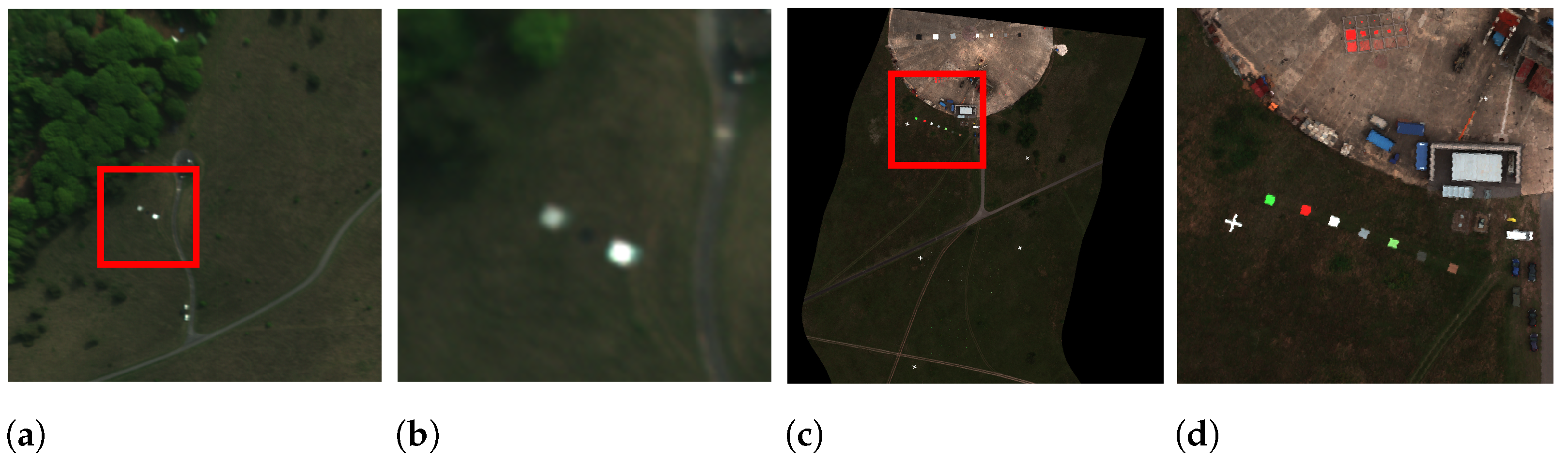
2.2. Image Acquisition
2.3. Spectral Dimensionality Reduction Techniques
2.3.1. Principal Component Analysis
2.3.2. Maximum Noise Fraction
2.3.3. Folded Principal Component Analysis
2.3.4. Independent Component Analysis
2.4. Spatial Dimensionality Reduction Using Vegetation Indices
2.5. Target Detection Algorithms
2.6. Performance Measures
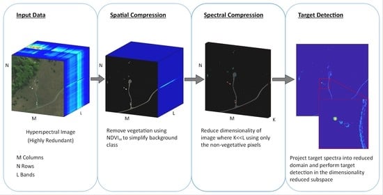
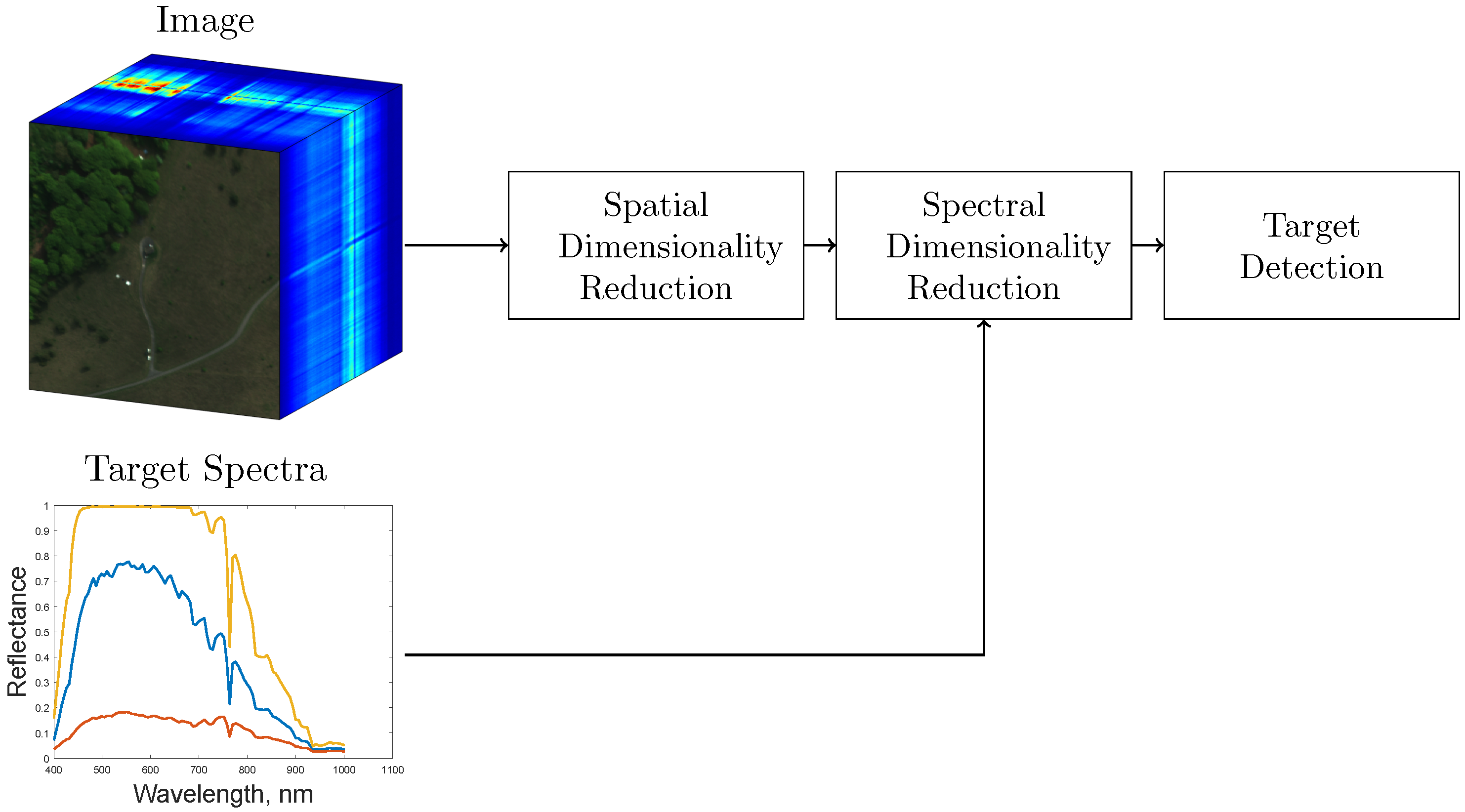
2.7. Proposed Methodology
3. Experimental Results
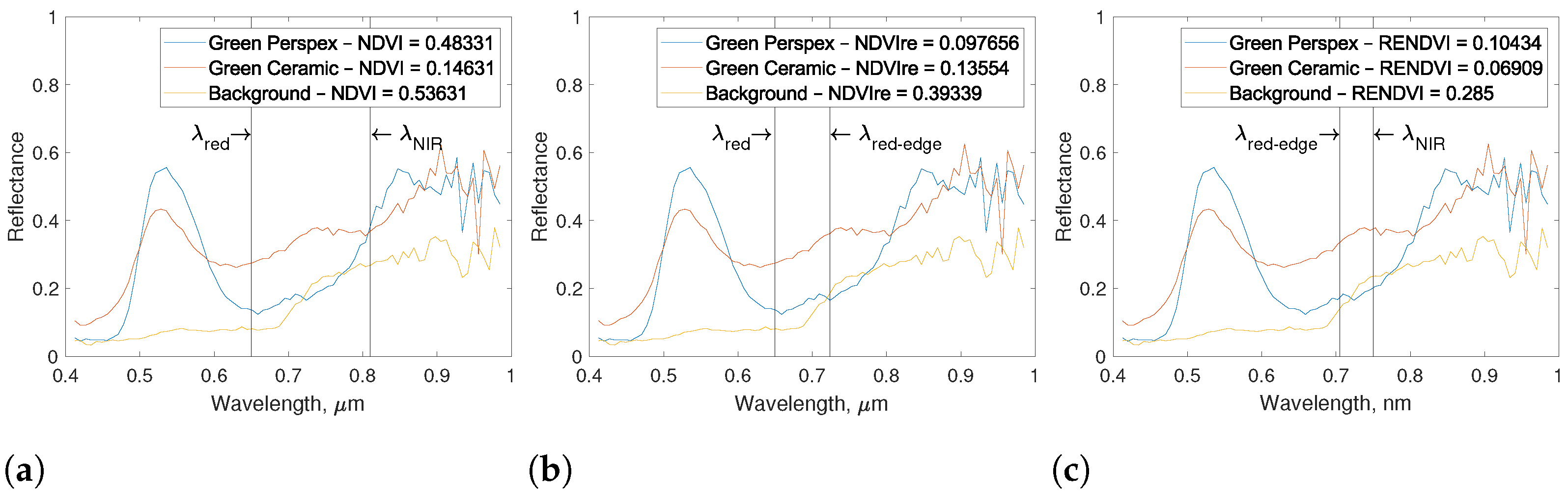
3.1. Selection of the Optimal Vegetation Index for Spatial Dimensionality Reduction
3.2. Combining Spatial and Spectral DR for Hyperspectral Compression
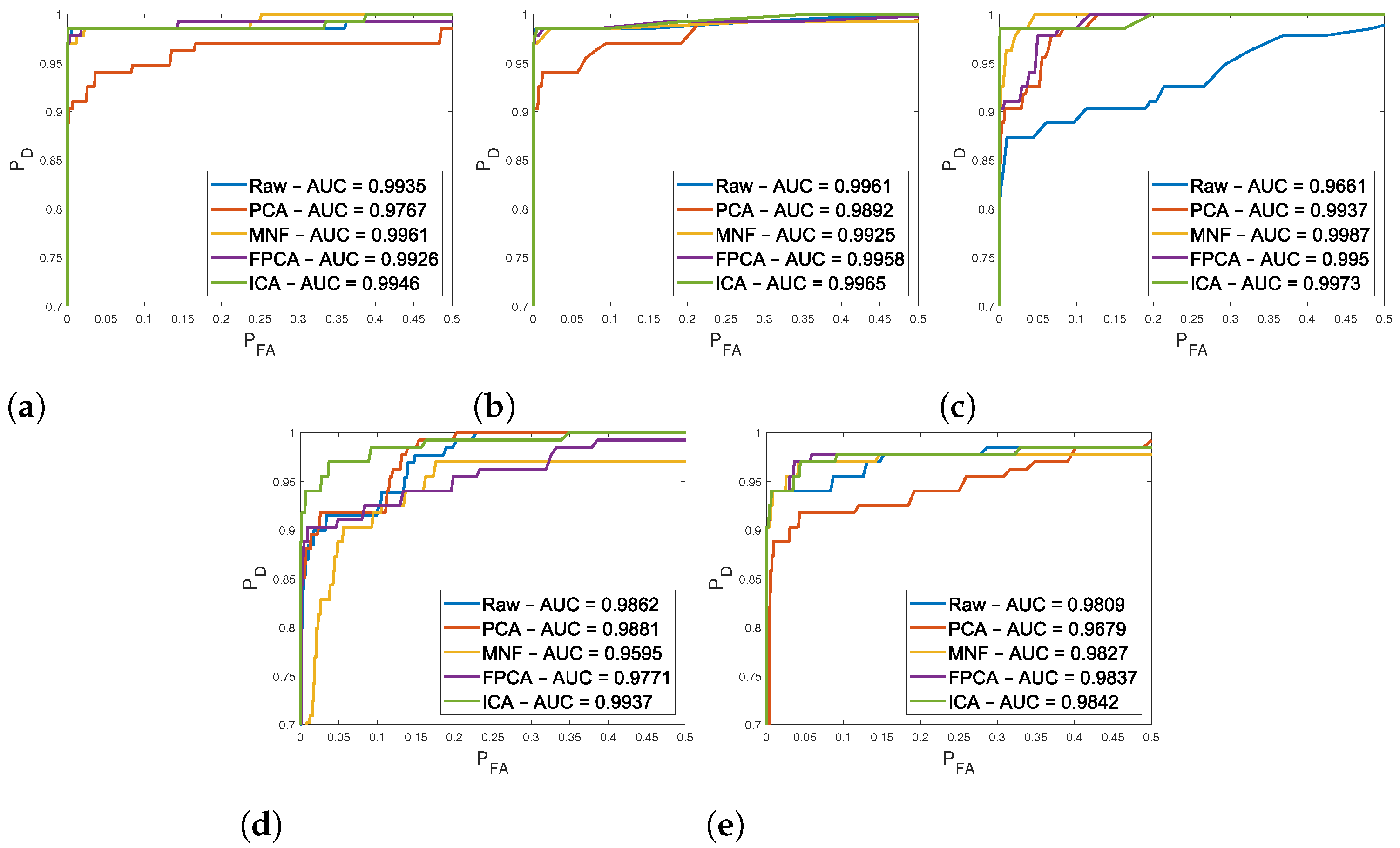
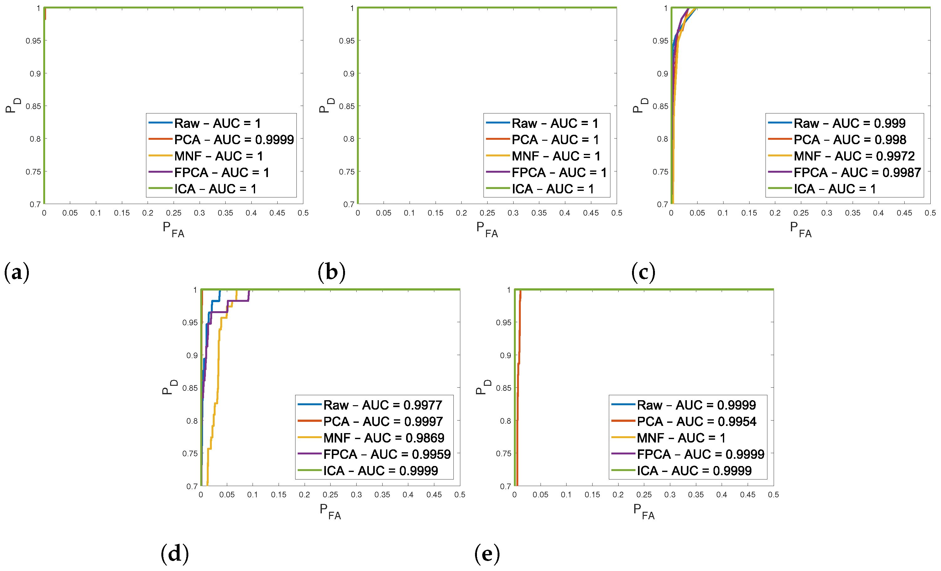
3.3. Comparison of the TD Algorithms Used
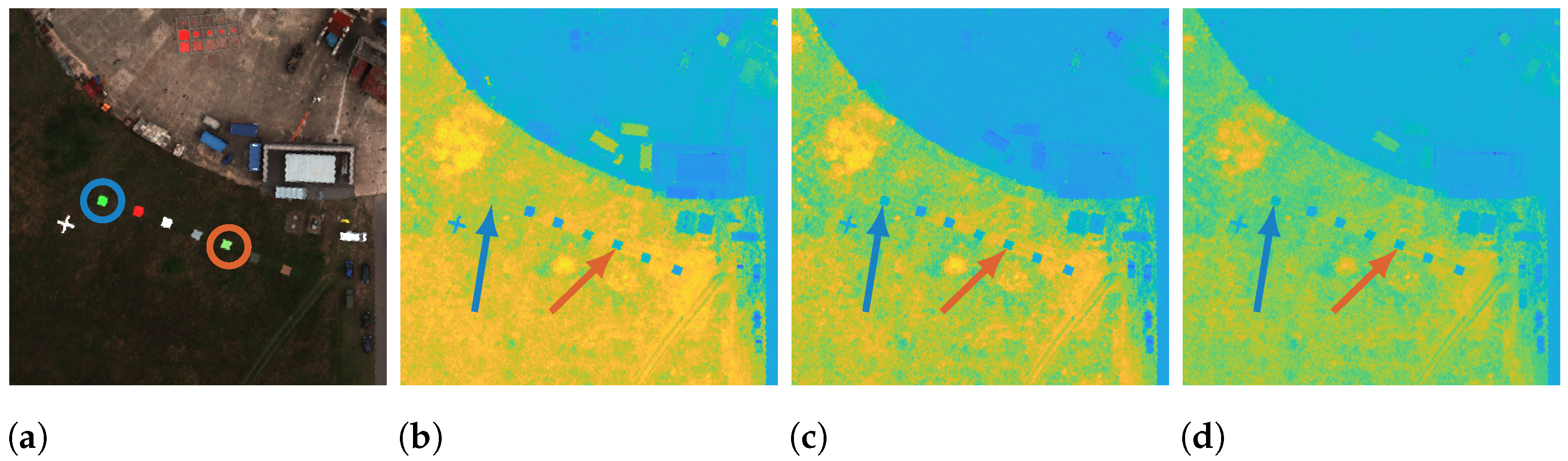
3.4. Results on the OP7 Dataset
3.5. Results on the UDRC Selene Dataset
4. Discussion
- K must be a factor of the total number of wavelengths L or
- When selecting the folding parameters H and W,
5. Conclusions
Author Contributions
Funding
Acknowledgments
Conflicts of Interest
Abbreviations
| ACE | Adaptive Cosine Estimator |
| AD | Anomaly Detection |
| AUC | Area Under the Curve |
| CEM | Constrained Energy Minimisation |
| DR | Dimensionality Reduction |
| EVD | Eigenvalue Decomposition |
| FAR | False Alarm Rate |
| FN | False Negative |
| FNR | False Negative Rate |
| FP | False Positive |
| FPCA | Folded Principal Component Analysis |
| FPR | False Positive Rate |
| GSD | Ground Sample Distance |
| IC | Independent Components |
| ICA | Independent Component Analysis |
| MCC | Matthew’s Correlation Coefficient |
| MNF | Maximum Noise Fraction |
| NDVI | Normalised Difference Vegetation Index |
| NDVI | Normalised Difference Vegetation Index (red-edge) |
| NDWI | Normalised Difference Water Index |
| NDSI | Normalised Difference Snow Index |
| NIPALS | Non-linear Iterative Partial Least Squares |
| NIR | Near-InfraRed |
| OSP | Orthogonal Subspace Projection |
| P | Probability of Detection |
| P | Probability of False Alarm |
| PC | Principal Components |
| PCA | Principal Component Analysis |
| PR | Precision-Recall |
| RENDVI | Red Edge Normalised Difference Vegetation Index |
| ROC | Receiver Operator Characteristic |
| RXD | Reed-Xiaoli Detector |
| SAM | Spectral Angle Mapper |
| SID | Spectral Information Divergence |
| SNR | Signal-to-Noise Ratio |
| TD | Target Detection |
| TN | True Negative |
| TNR | True Negative Rate |
| TP | True Positive |
| TPR | True Positive Rate |
| VD | Virtual Dimensionality |
| VI | Vegetation Indices |
| VNIR | Visible and Near-InfraRed |
References
- Van Aardt, J.A.; McKeown, D.; Faulring, J.; Raqueño, N.; Casterline, M.; Renschler, C.; Eguchi, R.; Messinger, D.; Krzaczek, R.; Cavillia, S. Geospatial disaster response during the Haiti earthquake: A case study spanning airborne deployment, data collection, transfer, processing, and dissemination. Photogramm. Eng. Remote Sens. 2011, 77, 943–952. [Google Scholar] [CrossRef] [Green Version]
- Ettehadi Osgouei, P.; Kaya, S.; Sertel, E.; Alganci, U. Separating Built-Up Areas from Bare Land in Mediterranean Cities Using Sentinel-2A Imagery. Remote Sens. 2019, 11, 345. [Google Scholar] [CrossRef] [Green Version]
- Xue, J.; Su, B. Significant remote sensing vegetation indices: A review of developments and applications. J. Sens. 2017, 2017, 1353691. [Google Scholar] [CrossRef] [Green Version]
- Theiler, J.; Kucer, M.; Ziemann, A. Experiments in anomalous change detection with the Viareggio 2013 trial dataset. In Algorithms, Technologies, and Applications for Multispectral and Hyperspectral Imagery XXVI; International Society for Optics and Photonics: Bellingham, WA, USA, 2020; Volume 11392, p. 1139211. [Google Scholar]
- Ghaderpour, E.; Vujadinovic, T. Change Detection within Remotely Sensed Satellite Image Time Series via Spectral Analysis. Remote Sens. 2020, 12, 4001. [Google Scholar] [CrossRef]
- Kwan, C.; Chou, B.; Yang, J.; Tran, T. Compressive object tracking and classification using deep learning for infrared videos. In Pattern Recognition and Tracking XXX; International Society for Optics and Photonics: Washington, DC, USA, 2019; Volume 10995, p. 1099506. [Google Scholar]
- Manolakis, D.; Truslow, E.; Pieper, M.; Cooley, T.; Brueggeman, M. Detection algorithms in hyperspectral imaging systems: An overview of practical algorithms. IEEE Signal Process. Mag. 2013, 31, 24–33. [Google Scholar] [CrossRef]
- Chang, C.I. Hyperspectral target detection. In Real-Time Progressive Hyperspectral Image Processing; Springer: Berlin/Heidelberg, Germany, 2016; pp. 131–172. [Google Scholar]
- Wang, Q.; Lin, Q.; Li, M.; Tian, Q. A new target detection algorithm: Spectra sort encoding. Int. J. Remote Sens. 2009, 30, 2297–2307. [Google Scholar] [CrossRef]
- Nasrabadi, N.M. Hyperspectral target detection: An overview of current and future challenges. IEEE Signal Process. Mag. 2014, 31, 34–44. [Google Scholar] [CrossRef]
- Manolakis, D.; Lockwood, R.; Cooley, T.; Jacobson, J. Is there a best hyperspectral detection algorithm? In Algorithms and Technologies for Multispectral, Hyperspectral, and Ultraspectral Imagery XV; International Society for Optics and Photonics: Bellingham, WA, USA, 2009; Volume 7334, p. 733402. [Google Scholar]
- Chang, C.I.; Cao, H.; Chen, S.; Shang, X.; Yu, C.; Song, M. Orthogonal Subspace Projection-Based Go-Decomposition Approach to Finding Low-Rank and Sparsity Matrices for Hyperspectral Anomaly Detection. IEEE Trans. Geosci. Remote Sens. 2020. [Google Scholar] [CrossRef]
- Chang, C.I. Hyperspectral Imaging: Techniques for Spectral Detection and Classification; Springer Science & Business Media: Berlin/Heidelberg, Germany, 2003; Volume 1. [Google Scholar]
- Jin, X.; Paswaters, S.; Cline, H. A comparative study of target detection algorithms for hyperspectral imagery. In Algorithms and Technologies for Multispectral, Hyperspectral, and Ultraspectral Imagery XV; International Society for Optics and Photonics: Bellingham, WA, USA, 2009; Volume 7334, p. 73341W. [Google Scholar]
- Olson, C.; Nichols, J.; Michalowicz, J.; Bucholtz, F. Improved Outlier Identification in Hyperspectral Imaging via Nonlinear Dimensionality Reduction; SPIE Defense, Security, and Sensing; SPIE: Bellingham, WA, USA, 2010; Volume 7695. [Google Scholar]
- Manolakis, D.; Pieper, M.; Truslow, E.; Cooley, T.; Brueggeman, M.; Lipson, S. The remarkable success of adaptive cosine estimator in hyperspectral target detection. In Algorithms and Technologies for Multispectral, Hyperspectral, and Ultraspectral Imagery XIX; International Society for Optics and Photonics: Bellingham, WA, USA, 2013; Volume 8743, p. 874302. [Google Scholar]
- Bakken, S.; Orlandic, M.; Johansen, T.A. The effect of dimensionality reduction on signature-based target detection for hyperspectral remote sensing. In CubeSats and SmallSats for Remote Sensing III; International Society for Optics and Photonics: Bellingham, WA, USA, 2019; Volume 11131, p. 111310L. [Google Scholar]
- Macfarlane, F.; Murray, P.; Marshall, S.; White, H. A Fast Hyperspectral Hit-or-Miss Transform with Integrated Projection-Based Dimensionality Reduction. Hyperspectral Imaging HSI 2018. Available online: https://strathprints.strath.ac.uk/65308/ (accessed on 12 November 2020).
- Macfarlane, F.; Murray, P.; Marshall, S.; White, H. Object Detection and Classification in Aerial Hyperspectral Imagery Using a Multivariate Hit-or-Miss Transform; SPIE Defense + Commercial Sensing; SPIE: Bellingham, WA, USA, 2019; Volume 10986. [Google Scholar]
- Abdi, H.; Williams, L.J. Principal component analysis. Wiley Interdiscip. Rev. Comput. Stat. 2010, 2, 433–459. [Google Scholar] [CrossRef]
- Andrecut, M. Parallel GPU implementation of iterative PCA algorithms. J. Comput. Biol. 2009, 16, 1593–1599. [Google Scholar] [CrossRef] [Green Version]
- Green, A.A.; Berman, M.; Switzer, P.; Craig, M.D. A transformation for ordering multispectral data in terms of image quality with implications for noise removal. IEEE Trans. Geosci. Remote Sens. 1988, 26, 65–74. [Google Scholar] [CrossRef] [Green Version]
- Luo, G.; Chen, G.; Tian, L.; Qin, K.; Qian, S.E. Minimum Noise Fraction versus Principal Component Analysis as a Preprocessing Step for Hyperspectral Imagery Denoising. Can. J. Remote Sens. 2016, 42, 106–116. [Google Scholar] [CrossRef]
- Zabalza, J.; Ren, J.; Yang, M.; Zhang, Y.; Wang, J.; Marshall, S.; Han, J. Novel Folded-PCA for improved feature extraction and data reduction with hyperspectral imaging and SAR in remote sensing. ISPRS J. Photogramm. Remote Sens. 2014, 93, 112–122. [Google Scholar] [CrossRef] [Green Version]
- Cao, L.J.; Chua, K.S.; Chong, W.K.; Lee, H.P.; Gu, Q.M. A comparison of PCA, KPCA and ICA for dimensionality reduction in support vector machine. Neurocomputing 2003, 55, 321–336. [Google Scholar] [CrossRef]
- Hyvärinen, A.; Oja, E. A fast fixed-point algorithm for independent component analysis. Neural Comput. 1997, 9, 1483–1492. [Google Scholar] [CrossRef]
- Cardoso, J.F.; Souloumiac, A. Blind beamforming for non-Gaussian signals. In IEE Proceedings F (Radar and Signal Processing); IET: London, UK, 1993; Volume 140, pp. 362–370. [Google Scholar]
- Chang, C. A Review of Virtual Dimensionality for Hyperspectral Imagery. IEEE J. Sel. Top. Appl. Earth Obs. Remote Sens. 2018, 11, 1285–1305. [Google Scholar] [CrossRef]
- Wang, J.; Chang, C. Applications of Independent Component Analysis in Endmember Extraction and Abundance Quantification for Hyperspectral Imagery. IEEE Trans. Geosci. Remote Sens. 2006, 44, 2601–2616. [Google Scholar] [CrossRef]
- Rouse, J.W., Jr.; Haas, R.H.; Schell, J.; Deering, D. Monitoring the Vernal Advancement and Retrogradation (Green Wave Effect) of Natural Vegetation 1973. Available online: https://core.ac.uk/download/pdf/42887948.pdf (accessed on 5 January 2021).
- Hansen, P.; Schjoerring, J. Reflectance measurement of canopy biomass and nitrogen status in wheat crops using normalized difference vegetation indices and partial least squares regression. Remote Sens. Environ. 2003, 86, 542–553. [Google Scholar] [CrossRef]
- Gitelson, A.; Merzlyak, M.N. Spectral reflectance changes associated with autumn senescence of Aesculus hippocastanum L. and Acer platanoides L. leaves. Spectral features and relation to chlorophyll estimation. J. Plant Physiol. 1994, 143, 286–292. [Google Scholar] [CrossRef]
- Sims, D.A.; Gamon, J.A. Relationships between leaf pigment content and spectral reflectance across a wide range of species, leaf structures and developmental stages. Remote Sens. Environ. 2002, 81, 337–354. [Google Scholar] [CrossRef]
- Kraut, S.; Scharf, L.L.; Butler, R.W. The adaptive coherence estimator: A uniformly most-powerful-invariant adaptive detection statistic. IEEE Trans. Signal Process. 2005, 53, 427–438. [Google Scholar] [CrossRef]
- Kruse, F.A.; Lefkoff, A.; Boardman, J.; Heidebrecht, K.; Shapiro, A.; Barloon, P.; Goetz, A. The spectral image processing system (SIPS)—interactive visualization and analysis of imaging spectrometer data. Remote Sens. Environ. 1993, 44, 145–163. [Google Scholar] [CrossRef]
- Chang, C.I. Spectral information divergence for hyperspectral image analysis. In Proceedings of the IEEE 1999 International Geoscience and Remote Sensing Symposium, IGARSS’99 (Cat. No. 99CH36293), Hamburg, Germany, 28 June–2 July 1999; IEEE: Piscataway, NJ, USA, 1999; Volume 1, pp. 509–511. [Google Scholar]
- Reed, I.S.; Yu, X. Adaptive multiple-band CFAR detection of an optical pattern with unknown spectral distribution. IEEE Trans. Acoust. Speech Signal Process. 1990, 38, 1760–1770. [Google Scholar] [CrossRef]
- Chang, C.I.; Chen, J. Orthogonal Subspace Projection Using Data Sphering and Low-Rank and Sparse Matrix Decomposition for Hyperspectral Target Detection. IEEE Trans. Geosci. Remote Sens. 2021, 1–19. [Google Scholar] [CrossRef]
- Chang, C.I. Orthogonal subspace projection (OSP) revisited: A comprehensive study and analysis. IEEE Trans. Geosci. Remote Sens. 2005, 43, 502–518. [Google Scholar] [CrossRef]
- Shen, S.S.; Bajorski, P.; Lewis, P.E. Impact of missing endmembers on the performance of the OSP detector for hyperspectral images. In Algorithms and Technologies for Multispectral, Hyperspectral, and Ultraspectral Imagery XIII; International Society for Optics and Photonics: Bellingham, WA, USA, 2007. [Google Scholar] [CrossRef]
- Bajorski, P. Analytical Comparison of the Matched Filter and Orthogonal Subspace Projection Detectors for Hyperspectral Images. IEEE Trans. Geosci. Remote Sens. 2007, 45, 2394–2402. [Google Scholar] [CrossRef]
- Bajorski, P. Target Detection Under Misspecified Models in Hyperspectral Images. IEEE J. Sel. Top. Appl. Earth Obs. Remote Sens. 2012, 5, 470–477. [Google Scholar] [CrossRef]
- Gross, W.; Boehler, J.; Schilling, H.; Middelmann, W.; Weyermann, J.; Wellig, P.; Oechslin, R.; Kneubühler, M. Assessment of target detection limits in hyperspectral data. In Target and Background Signatures; International Society for Optics and Photonics: Bellingham, WA, USA, 2015; Volume 9653, p. 96530J. [Google Scholar]
- Kerekes, J. Receiver operating characteristic curve confidence intervals and regions. IEEE Geosci. Remote Sens. Lett. 2008, 5, 251–255. [Google Scholar] [CrossRef] [Green Version]
- Saito, T.; Rehmsmeier, M. The precision-recall plot is more informative than the ROC plot when evaluating binary classifiers on imbalanced datasets. PLoS ONE 2015, 10, e0118432. [Google Scholar]
- Powers, D.M. Evaluation: From precision, recall and F-measure to ROC, informedness, markedness and correlation. arXiv 2020, arXiv:2010.16061. [Google Scholar]
- Matthews, B.W. Comparison of the predicted and observed secondary structure of T4 phage lysozyme. Biochim. Biophys. Acta (BBA) Protein Struct. 1975, 405, 442–451. [Google Scholar] [CrossRef]
- Brodersen, K.H.; Ong, C.S.; Stephan, K.E.; Buhmann, J.M. The balanced accuracy and its posterior distribution. In Proceedings of the 2010 20th international conference on pattern recognition, Istanbul, Turkey, 23–26 August 2010; IEEE: Piscataway, NJ, USA, 2010; pp. 3121–3124. [Google Scholar]
- Verdoja, F.; Grangetto, M. Graph Laplacian for image anomaly detection. Mach. Vis. Appl. 2020, 31, 1–16. [Google Scholar] [CrossRef] [Green Version]


| Index | Acronym | Equation | Reference |
|---|---|---|---|
| Normalised Difference Vegetation Index | NDVI | Rouse et al. [30] | |
| Normalised Difference Vegetation Index (red-edge) | NDVIre | Hansen & Schjoerring [31] Ettehadi et al. [2] | |
| Red-Edge Normalised Difference Vegetation Index | RENDVI | Gitelson & Merzlyak [32] Sims & Gamon [33] |
| Vegetation Index | Green Perspex Ratio | Green Carpet Ratio | Background Ratio |
|---|---|---|---|
| NDVI | 0.48 | 0.14 | 0.53 |
| NDVIre | 0.09 | 0.13 | 0.39 |
| RENDVI | 0.10 | 0.06 | 0.28 |
| Image | # Samples Full | # Samples NDVIre | L | K | Spatial Comp. (%) | Spectral Comp. (%) | Total Comp. (%) | Average Comp. (%) |
|---|---|---|---|---|---|---|---|---|
| OP7_1 | 160,000 | 3504 | 100 | 20 | 2.19 | 20 | 0.44 | 0.34 |
| OP7_2 | 160,000 | 2500 | 100 | 20 | 1.56 | 20 | 0.31 | |
| OP7_3 | 160,000 | 2232 | 100 | 20 | 1.40 | 20 | 0.28 | |
| IM_140804 | 3,210,191 | 649,435 | 80 | 20 | 20.23 | 25 | 5.06 | 4.61 |
| IM_140806 | 3,839,976 | 578,674 | 80 | 20 | 15.07 | 25 | 3.77 | |
| IM_140807 | 3,415,052 | 689,245 | 80 | 20 | 20.18 | 25 | 5.05 | |
| IM_140808 | 3,015,944 | 543,569 | 80 | 20 | 18.02 | 25 | 4.51 | |
| IM_140812 | 4,360,159 | 610,172 | 80 | 20 | 13.99 | 25 | 3.50 | |
| IM_140813 | 3,301,404 | 807,262 | 80 | 20 | 24.45 | 25 | 6.11 | |
| IM_140815 | 3,640,769 | 626,776 | 80 | 20 | 17.22 | 25 | 4.30 |
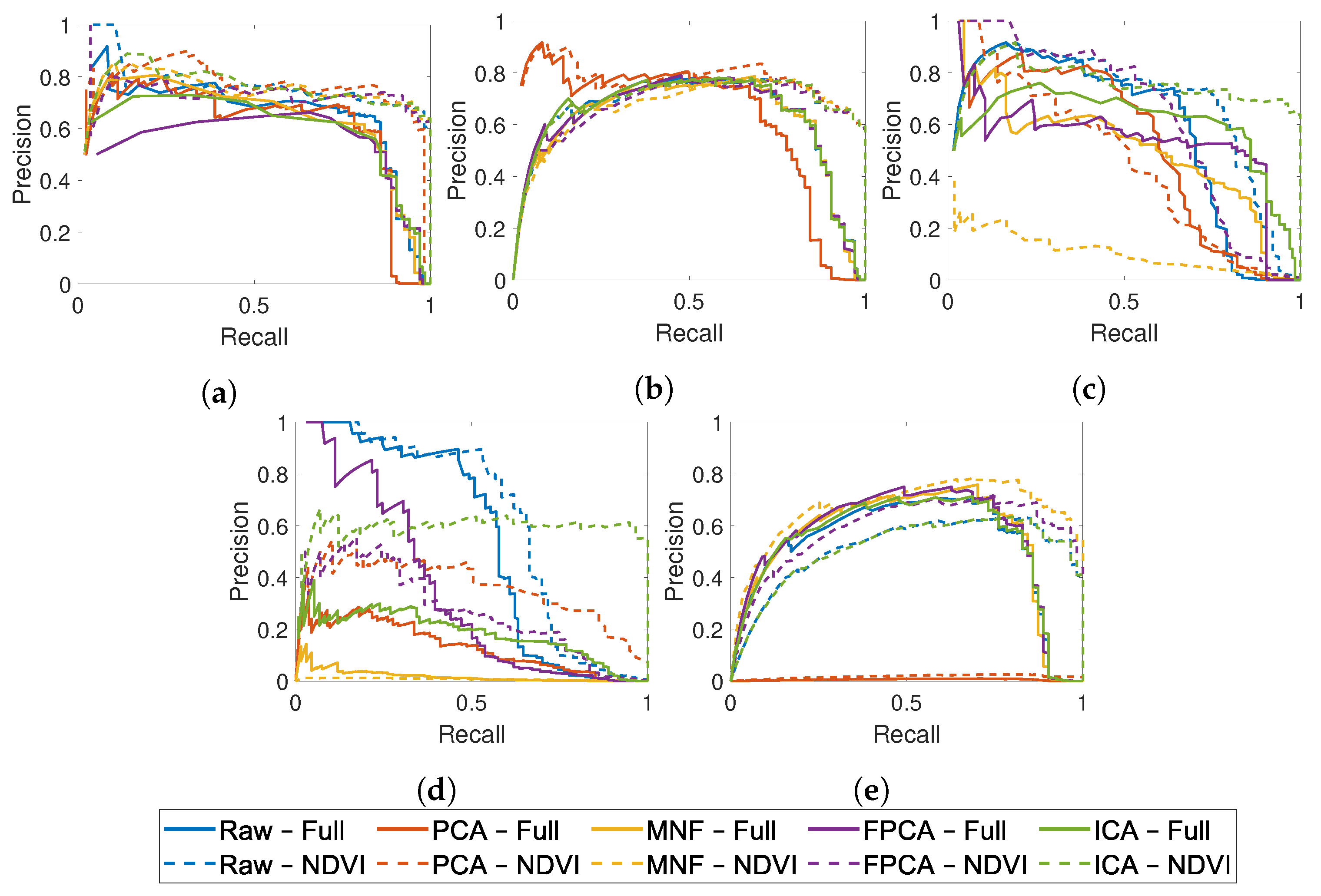
| PR | Raw | PCA | MNF | FPCA | ICA | |||||
|---|---|---|---|---|---|---|---|---|---|---|
| AUC | Full | NDVIre | Full | NDVIre | Full | NDVIre | Full | NDVIre | Full | NDVIre |
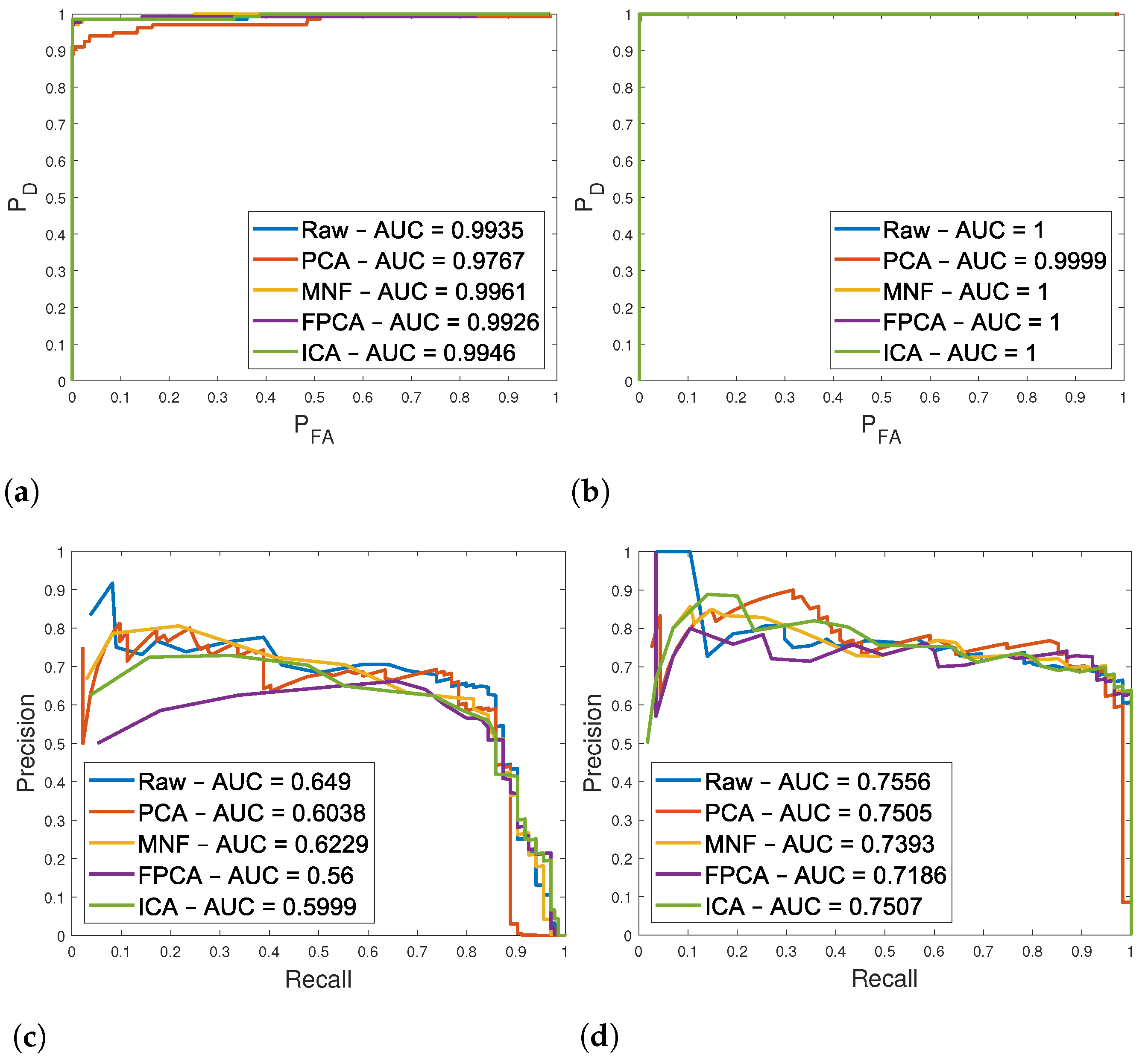
| ACE | 0.649 | 0.7556 | 0.6038 | 0.7505 | 0.6229 | 0.7393 | 0.56 | 0.7186 | 0.5999 | 0.7507 |
| CEM | 0.6207 | 0.6852 | 0.6208 | 0.7673 | 0.6033 | 0.6633 | 0.6124 | 0.6669 | 0.6195 | 0.6849 |
| SAM | 0.577 | 0.6723 | 0.5127 | 0.4443 | 0.4938 | 0.0993 | 0.528 | 0.6194 | 0.6006 | 0.7507 |
| SID | 0.5315 | 0.6112 | 0.131 | 0.3582 | 0.0187 | 0.0102 | 0.3314 | 0.2625 | 0.1809 | 0.5871 |
| RXD | 0.5153 | 0.5086 | 0.0055 | 0.0175 | 0.5358 | 0.6604 | 0.5445 | 0.5816 | 0.5224 | 0.5049 |
| ACE-Full | |||||||||
|---|---|---|---|---|---|---|---|---|---|
| K = 20 | DR | AUC ROC | AUC PR | Visibility | Precision | Recall | Bacc | F1 | MCC |
| Grey Tile | Raw | 1.00 | 0.84 | 0.88 | 0.37 | 0.88 | 0.93 | 0.35 | 0.43 |
| PCA | 1.00 | 0.77 | 0.94 | 0.12 | 0.95 | 0.96 | 0.12 | 0.18 | |
| MNF | 1.00 | 0.79 | 0.93 | 0.15 | 0.95 | 0.96 | 0.15 | 0.21 | |
| FPCA | 1.00 | 0.80 | 0.92 | 0.17 | 0.94 | 0.96 | 0.17 | 0.23 | |
| ICA | 1.00 | 0.78 | 0.93 | 0.16 | 0.95 | 0.96 | 0.16 | 0.23 | |
| Black Tile | Raw | 1.00 | 0.06 | 0.60 | 0.09 | 0.62 | 0.80 | 0.06 | 0.11 |
| PCA | 1.00 | 0.10 | 0.68 | 0.05 | 0.72 | 0.84 | 0.05 | 0.09 | |
| MNF | 1.00 | 0.15 | 0.70 | 0.09 | 0.75 | 0.85 | 0.07 | 0.12 | |
| FPCA | 1.00 | 0.13 | 0.71 | 0.05 | 0.76 | 0.85 | 0.05 | 0.09 | |
| ICA | 1.00 | 0.11 | 0.67 | 0.04 | 0.72 | 0.83 | 0.05 | 0.09 | |
| White Tile | Raw | 1.00 | 0.74 | 0.79 | 0.57 | 0.79 | 0.89 | 0.53 | 0.59 |
| PCA | 1.00 | 0.67 | 0.93 | 0.22 | 0.94 | 0.96 | 0.28 | 0.37 | |
| MNF | 1.00 | 0.68 | 0.85 | 0.39 | 0.86 | 0.92 | 0.41 | 0.47 | |
| FPCA | 1.00 | 0.60 | 0.83 | 0.33 | 0.84 | 0.91 | 0.35 | 0.41 | |
| ICA | 1.00 | 0.67 | 0.79 | 0.47 | 0.80 | 0.89 | 0.44 | 0.49 | |
| All Spectra | Raw | 1.00 | 0.55 | 0.76 | 0.34 | 0.77 | 0.87 | 0.32 | 0.37 |
| PCA | 1.00 | 0.52 | 0.85 | 0.13 | 0.87 | 0.92 | 0.15 | 0.22 | |
| MNF | 1.00 | 0.54 | 0.83 | 0.21 | 0.85 | 0.91 | 0.21 | 0.27 | |
| FPCA | 1.00 | 0.51 | 0.82 | 0.18 | 0.85 | 0.91 | 0.19 | 0.25 | |
| ICA | 1.00 | 0.52 | 0.80 | 0.22 | 0.82 | 0.89 | 0.22 | 0.27 | |
| ACE-NDVIre | |||||||||
|---|---|---|---|---|---|---|---|---|---|
| K = 20 | DR | AUC ROC | AUC PR | Visibility | Precision | Recall | Bacc | F1 | MCC |
| Grey Tile | Raw | 1.00 | 0.86 | 0.72 | 0.73 | 0.74 | 0.86 | 0.59 | 0.65 |
| PCA | 1.00 | 0.83 | 0.75 | 0.56 | 0.79 | 0.87 | 0.48 | 0.54 | |
| MNF | 1.00 | 0.85 | 0.76 | 0.56 | 0.80 | 0.87 | 0.48 | 0.54 | |
| FPCA | 1.00 | 0.84 | 0.81 | 0.54 | 0.84 | 0.90 | 0.51 | 0.57 | |
| ICA | 1.00 | 0.75 | 0.73 | 0.52 | 0.77 | 0.86 | 0.43 | 0.50 | |
| Black Tile | Raw | 0.98 | 0.37 | 0.52 | 0.40 | 0.57 | 0.76 | 0.25 | 0.33 |
| PCA | 0.94 | 0.08 | 0.48 | 0.06 | 0.56 | 0.74 | 0.09 | 0.14 | |
| MNF | 0.96 | 0.09 | 0.46 | 0.07 | 0.54 | 0.73 | 0.09 | 0.14 | |
| FPCA | 0.94 | 0.09 | 0.47 | 0.08 | 0.54 | 0.73 | 0.10 | 0.15 | |
| ICA | 0.93 | 0.08 | 0.42 | 0.05 | 0.49 | 0.71 | 0.08 | 0.12 | |
| White Tile | Raw | 0.97 | 0.66 | 0.57 | 0.83 | 0.58 | 0.78 | 0.58 | 0.63 |
| PCA | 0.95 | 0.61 | 0.59 | 0.78 | 0.60 | 0.79 | 0.59 | 0.63 | |
| MNF | 0.95 | 0.62 | 0.61 | 0.74 | 0.62 | 0.80 | 0.58 | 0.62 | |
| FPCA | 0.92 | 0.59 | 0.59 | 0.64 | 0.61 | 0.79 | 0.51 | 0.55 | |
| ICA | 0.94 | 0.63 | 0.57 | 0.73 | 0.59 | 0.78 | 0.53 | 0.58 | |
| All Spectra | Raw | 0.98 | 0.63 | 0.61 | 0.65 | 0.63 | 0.80 | 0.47 | 0.53 |
| PCA | 0.96 | 0.50 | 0.61 | 0.47 | 0.65 | 0.80 | 0.39 | 0.44 | |
| MNF | 0.97 | 0.52 | 0.61 | 0.46 | 0.65 | 0.80 | 0.38 | 0.44 | |
| FPCA | 0.96 | 0.50 | 0.62 | 0.42 | 0.66 | 0.81 | 0.37 | 0.43 | |
| ICA | 0.96 | 0.49 | 0.57 | 0.43 | 0.62 | 0.78 | 0.35 | 0.40 | |
| ACE-Full | |||||||||
|---|---|---|---|---|---|---|---|---|---|
| K = 20 | DR | AUC ROC | AUC PR | Visibility | Precision | Recall | Bacc | F1 | MCC |
| Brown Carpet | Raw | 0.97 | 0.33 | 0.65 | 0.19 | 0.67 | 0.82 | 0.17 | 0.24 |
| PCA | 0.97 | 0.06 | 0.60 | 0.04 | 0.64 | 0.80 | 0.03 | 0.07 | |
| MNF | 0.97 | 0.46 | 0.75 | 0.17 | 0.78 | 0.87 | 0.15 | 0.21 | |
| FPCA | 0.97 | 0.55 | 0.75 | 0.22 | 0.78 | 0.87 | 0.20 | 0.26 | |
| ICA | 0.97 | 0.57 | 0.75 | 0.25 | 0.78 | 0.87 | 0.22 | 0.28 | |
| Green Carpet | Raw | 0.98 | 0.61 | 0.82 | 0.32 | 0.83 | 0.91 | 0.36 | 0.43 |
| PCA | 0.95 | 0.07 | 0.45 | 0.06 | 0.51 | 0.72 | 0.03 | 0.06 | |
| MNF | 0.98 | 0.54 | 0.80 | 0.23 | 0.83 | 0.89 | 0.24 | 0.30 | |
| FPCA | 0.98 | 0.58 | 0.85 | 0.25 | 0.89 | 0.92 | 0.29 | 0.35 | |
| ICA | 0.98 | 0.60 | 0.86 | 0.22 | 0.90 | 0.92 | 0.27 | 0.32 | |
| Green Ceramic | Raw | 0.99 | 0.65 | 0.94 | 0.19 | 0.94 | 0.96 | 0.29 | 0.39 |
| PCA | 0.98 | 0.60 | 0.85 | 0.16 | 0.89 | 0.92 | 0.19 | 0.26 | |
| MNF | 0.99 | 0.60 | 0.93 | 0.13 | 0.95 | 0.96 | 0.20 | 0.29 | |
| FPCA | 0.99 | 0.54 | 0.94 | 0.12 | 0.96 | 0.96 | 0.20 | 0.30 | |
| ICA | 0.99 | 0.52 | 0.94 | 0.13 | 0.96 | 0.96 | 0.20 | 0.30 | |
| Green Perspex | Raw | 1.00 | 0.63 | 0.95 | 0.22 | 0.95 | 0.97 | 0.32 | 0.42 |
| PCA | 0.99 | 0.44 | 0.91 | 0.08 | 0.93 | 0.95 | 0.12 | 0.20 | |
| MNF | 1.00 | 0.55 | 0.95 | 0.16 | 0.97 | 0.97 | 0.24 | 0.33 | |
| FPCA | 1.00 | 0.51 | 0.95 | 0.16 | 0.97 | 0.97 | 0.25 | 0.34 | |
| ICA | 1.00 | 0.57 | 0.96 | 0.15 | 0.97 | 0.97 | 0.23 | 0.33 | |
| Grey Ceramic | Raw | 0.99 | 0.61 | 0.77 | 0.31 | 0.78 | 0.88 | 0.27 | 0.34 |
| PCA | 0.98 | 0.47 | 0.81 | 0.13 | 0.83 | 0.90 | 0.11 | 0.17 | |
| MNF | 0.99 | 0.58 | 0.85 | 0.16 | 0.88 | 0.92 | 0.18 | 0.24 | |
| FPCA | 0.99 | 0.55 | 0.84 | 0.18 | 0.87 | 0.91 | 0.21 | 0.27 | |
| ICA | 0.99 | 0.53 | 0.82 | 0.18 | 0.85 | 0.90 | 0.19 | 0.25 | |
| Orange Perspex | Raw | 0.99 | 0.32 | 0.90 | 0.12 | 0.90 | 0.95 | 0.20 | 0.31 |
| PCA | 0.99 | 0.25 | 0.92 | 0.05 | 0.93 | 0.96 | 0.08 | 0.18 | |
| MNF | 0.99 | 0.29 | 0.93 | 0.07 | 0.94 | 0.96 | 0.13 | 0.24 | |
| FPCA | 0.99 | 0.30 | 0.93 | 0.08 | 0.94 | 0.96 | 0.14 | 0.25 | |
| ICA | 0.99 | 0.31 | 0.93 | 0.08 | 0.94 | 0.96 | 0.14 | 0.25 | |
| White Perspex | Raw | 0.98 | 0.07 | 0.48 | 0.07 | 0.49 | 0.74 | 0.05 | 0.10 |
| PCA | 0.99 | 0.27 | 0.83 | 0.04 | 0.85 | 0.91 | 0.05 | 0.11 | |
| MNF | 0.99 | 0.10 | 0.65 | 0.04 | 0.67 | 0.82 | 0.03 | 0.08 | |
| FPCA | 0.98 | 0.03 | 0.56 | 0.04 | 0.59 | 0.78 | 0.03 | 0.07 | |
| ICA | 0.98 | 0.02 | 0.45 | 0.03 | 0.49 | 0.72 | 0.02 | 0.05 | |
| All Spectra | Raw | 0.99 | 0.46 | 0.77 | 0.21 | 0.78 | 0.88 | 0.23 | 0.31 |
| PCA | 0.98 | 0.30 | 0.74 | 0.08 | 0.77 | 0.87 | 0.08 | 0.14 | |
| MNF | 0.99 | 0.46 | 0.82 | 0.14 | 0.85 | 0.91 | 0.16 | 0.23 | |
| FPCA | 0.99 | 0.45 | 0.82 | 0.16 | 0.84 | 0.90 | 0.19 | 0.26 | |
| ICA | 0.99 | 0.45 | 0.79 | 0.15 | 0.82 | 0.89 | 0.18 | 0.25 | |
| ACE-NDVIre | |||||||||
|---|---|---|---|---|---|---|---|---|---|
| K = 20 | DR | AUC ROC | AUC PR | Visibility | Precision | Recall | Bacc | F1 | MCC |
| Brown Carpet | Raw | 1.00 | 0.20 | 0.53 | 0.15 | 0.55 | 0.76 | 0.13 | 0.18 |
| PCA | 0.97 | 0.01 | 0.31 | 0.00 | 0.37 | 0.65 | 0.01 | 0.03 | |
| MNF | 0.99 | 0.15 | 0.56 | 0.12 | 0.61 | 0.78 | 0.09 | 0.14 | |
| FPCA | 0.99 | 0.27 | 0.59 | 0.17 | 0.64 | 0.79 | 0.13 | 0.18 | |
| ICA | 1.00 | 0.47 | 0.68 | 0.22 | 0.73 | 0.84 | 0.19 | 0.25 | |
| Green Carpet | Raw | 1.00 | 0.63 | 0.82 | 0.37 | 0.83 | 0.91 | 0.41 | 0.47 |
| PCA | 0.95 | 0.05 | 0.41 | 0.05 | 0.46 | 0.70 | 0.04 | 0.07 | |
| MNF | 1.00 | 0.48 | 0.75 | 0.24 | 0.79 | 0.87 | 0.24 | 0.31 | |
| FPCA | 1.00 | 0.58 | 0.82 | 0.30 | 0.86 | 0.91 | 0.32 | 0.38 | |
| ICA | 1.00 | 0.61 | 0.89 | 0.28 | 0.93 | 0.94 | 0.34 | 0.40 | |
| Green Ceramic | Raw | 1.00 | 0.70 | 0.96 | 0.37 | 0.96 | 0.97 | 0.49 | 0.56 |
| PCA | 1.00 | 0.63 | 0.91 | 0.25 | 0.93 | 0.95 | 0.30 | 0.38 | |
| MNF | 1.00 | 0.62 | 0.96 | 0.27 | 0.97 | 0.97 | 0.38 | 0.46 | |
| FPCA | 1.00 | 0.60 | 0.96 | 0.28 | 0.97 | 0.97 | 0.39 | 0.46 | |
| ICA | 1.00 | 0.62 | 0.96 | 0.30 | 0.98 | 0.98 | 0.42 | 0.49 | |
| Green Perspex | Raw | 1.00 | 0.68 | 0.97 | 0.41 | 0.97 | 0.98 | 0.54 | 0.60 |
| PCA | 1.00 | 0.61 | 0.96 | 0.23 | 0.98 | 0.98 | 0.31 | 0.38 | |
| MNF | 1.00 | 0.60 | 0.97 | 0.32 | 0.98 | 0.98 | 0.43 | 0.50 | |
| FPCA | 1.00 | 0.60 | 0.97 | 0.33 | 0.98 | 0.98 | 0.44 | 0.50 | |
| ICA | 1.00 | 0.64 | 0.97 | 0.33 | 0.98 | 0.98 | 0.44 | 0.51 | |
| Grey Ceramic | Raw | 1.00 | 0.62 | 0.73 | 0.40 | 0.75 | 0.86 | 0.35 | 0.41 |
| PCA | 1.00 | 0.47 | 0.76 | 0.22 | 0.79 | 0.87 | 0.19 | 0.26 | |
| MNF | 1.00 | 0.60 | 0.78 | 0.29 | 0.82 | 0.89 | 0.28 | 0.35 | |
| FPCA | 1.00 | 0.58 | 0.78 | 0.29 | 0.83 | 0.89 | 0.30 | 0.35 | |
| ICA | 1.00 | 0.60 | 0.79 | 0.28 | 0.83 | 0.89 | 0.27 | 0.34 | |
| Orange Perspex | Raw | 1.00 | 0.35 | 0.87 | 0.18 | 0.87 | 0.93 | 0.25 | 0.36 |
| PCA | 1.00 | 0.25 | 0.91 | 0.09 | 0.91 | 0.95 | 0.14 | 0.25 | |
| MNF | 1.00 | 0.35 | 0.92 | 0.11 | 0.93 | 0.95 | 0.18 | 0.29 | |
| FPCA | 1.00 | 0.33 | 0.92 | 0.12 | 0.92 | 0.95 | 0.18 | 0.30 | |
| ICA | 1.00 | 0.36 | 0.93 | 0.11 | 0.94 | 0.96 | 0.17 | 0.29 | |
| White Perspex | Raw | 0.98 | 0.11 | 0.41 | 0.10 | 0.43 | 0.70 | 0.08 | 0.12 |
| PCA | 0.99 | 0.24 | 0.72 | 0.10 | 0.75 | 0.85 | 0.09 | 0.16 | |
| MNF | 0.98 | 0.06 | 0.50 | 0.06 | 0.54 | 0.75 | 0.04 | 0.09 | |
| FPCA | 0.98 | 0.06 | 0.48 | 0.05 | 0.53 | 0.74 | 0.04 | 0.09 | |
| ICA | 0.94 | 0.02 | 0.35 | 0.02 | 0.41 | 0.67 | 0.02 | 0.05 | |
| All Spectra | Raw | 1.00 | 0.46 | 0.73 | 0.28 | 0.74 | 0.86 | 0.30 | 0.37 |
| PCA | 0.98 | 0.30 | 0.67 | 0.13 | 0.70 | 0.83 | 0.14 | 0.20 | |
| MNF | 0.99 | 0.40 | 0.75 | 0.20 | 0.78 | 0.87 | 0.22 | 0.28 | |
| FPCA | 0.99 | 0.43 | 0.76 | 0.22 | 0.79 | 0.88 | 0.24 | 0.31 | |
| ICA | 0.99 | 0.47 | 0.77 | 0.22 | 0.80 | 0.88 | 0.26 | 0.32 | |
Publisher’s Note: MDPI stays neutral with regard to jurisdictional claims in published maps and institutional affiliations. |
© 2021 by the authors. Licensee MDPI, Basel, Switzerland. This article is an open access article distributed under the terms and conditions of the Creative Commons Attribution (CC BY) license (https://creativecommons.org/licenses/by/4.0/).
Share and Cite
Macfarlane, F.; Murray, P.; Marshall, S.; White, H. Investigating the Effects of a Combined Spatial and Spectral Dimensionality Reduction Approach for Aerial Hyperspectral Target Detection Applications. Remote Sens. 2021, 13, 1647. https://0-doi-org.brum.beds.ac.uk/10.3390/rs13091647
Macfarlane F, Murray P, Marshall S, White H. Investigating the Effects of a Combined Spatial and Spectral Dimensionality Reduction Approach for Aerial Hyperspectral Target Detection Applications. Remote Sensing. 2021; 13(9):1647. https://0-doi-org.brum.beds.ac.uk/10.3390/rs13091647
Chicago/Turabian StyleMacfarlane, Fraser, Paul Murray, Stephen Marshall, and Henry White. 2021. "Investigating the Effects of a Combined Spatial and Spectral Dimensionality Reduction Approach for Aerial Hyperspectral Target Detection Applications" Remote Sensing 13, no. 9: 1647. https://0-doi-org.brum.beds.ac.uk/10.3390/rs13091647