1. Introduction
Land surface temperature (LST), controlled by land-atmosphere interactions and energy fluxes, is a key parameter in the earth’s climate [
1] and energy-water cycle at regional and global scales [
2,
3,
4]. LST drives and controls many biophysical processes between the hydrosphere, atmosphere, and biosphere [
5,
6], playing an important role in climate research and global change, such as monitoring glaciers, vegetation assessments, and terrestrial carbon flux research [
7,
8].
In situ derived LST data, which are assessed from various sources, such as meteorological stations and Argo floats, have the advantage of high reliability and a longer time series [
9]. However, in situ data measurements are often sparsely or/and irregularly distributed, especially in polar regions and mountainous areas [
10,
11].
Satellite LST data, which can be easily acquired with global coverage, provides the only opportunity of observing LSTs with sufficient spatial resolution and adequate time series [
3]. Over the past decade, satellite LST data have been widely used for glacial-hydro-climatological studies [
11,
12], permafrost mapping [
13,
14], environmental assessment [
15], and climate change [
16] in areas that lack ground-based LST data, such as the Himalayan region, the Tibetan Plateau, the Arctic, and Antarctica. The retrieval of LSTs from satellites is based on a variety of mature algorithms that have been proposed for thermal infrared (TIR) channels since the 1970s [
17]. Numerous satellite LST products have been developed from a variety of sensors [
18,
19]. The most widely used LST products from Moderate Resolution Imaging Spectroradiometer (MODIS) on Terra and Aqua satellites retrieved by the generalized split-window algorithm [
20] are available between February 2000 and July 2002, respectively. The MODIS LST products have the advantage of optimal spatial resolution (nominally 1 km), and high temporal resolution (four global coverages a day, at 10:30, 13:30, 22:30, 01:30 nominal time). The data has been validated by in situ LST measurement for various land cover types. The accuracy of MODIS LST products was better than 1 K at most stations [
4]. However, cloud cover can cause frequent missing data in satellite LST data. Research confirmed that more than 60% of the Earth’s surface is covered by clouds on any given day on average [
21], seriously restricting its applications to clear-sky conditions [
22]. Data gaps in satellite LST products impact understanding the magnitude of its trend [
23] and the absolute LST value compared with in situ data [
24]. The large differences in LST between clear-sky and cloudy-sky conditions limit its applications for climate change research [
24,
25].
To date, numerous methods have been developed for filling in LST gaps under cloudy-sky conditions to obtain a spatially and temporally continuous satellite LST product. Geostatistical interpolation is the most common spatially-based LST reconstruction method (e.g., the Kriging method and many improved Kriging methods) [
10]. Methods based on spatial correlations of cloudy-sky pixels with neighboring clear-sky pixels can only be applied to images with few cloud-covered pixels. The second type of cloudy-sky LST reconstruction method considers correlations in time [
26]. Based on the trend and seasonality of LST time series, the harmonic analysis of time series [
27] and the Savitzky-Golay filter method [
28,
29] have been used to build a temporal model by fitting available LST time series data at each point and then apply it to reconstruct cloudy-sky pixels. However, temporal approaches work best on seasonal LST changes and smooth diurnal LST variations [
30]. Thus, temporal approaches are not suitable for reconstructing the daily MODIS LST product, especially in areas with active land cover changes. Because LST is impacted by environmental factors such as vegetation and elevation, gap-filling reconstructs the cloudy pixel LST by building an empirical LST model with related environmental datasets such as normalized difference vegetation index (NDVI) and digital elevation model (DEM) [
26]. The reconstructed LST is impacted by the uncertainty of these auxiliary datasets and the accuracy of the empirical LST models. These methods of deriving the theoretical clear-sky LST are subject to system bias errors.
Many methods have been developed to derive actual cloudy-sky LST. The surface energy balance-based (EB) method was proposed to recover cloudy-sky LST based on its spatially and temporally neighboring valid pixels [
31,
32]. This method is based on the assumption that a cloudy pixel differs in temperature from its neighboring clear-sky pixels mainly because of their different surface incident radiation and redistributions. Therefore, cloudy-sky LST can be obtained based on its spatially and temporally neighboring clear-sky LST and a temperature correction term related to the surface incident radiation, atmospheric temperature, and wind velocity, which are usually not available at a global scale. The first operational all-weather LST product for MSG/SEVIRI derived at the Satellite Application Facility on Land Surface Analysis (LSA-SAF) through the EB method utilized the all-weather downward surface shortwave and longwave radiation flux products [
33,
34]. However, the LSA-SAF product doesn’t cover the Asian region and needs to be validated for additional land cover types. Many cloudy-sky LST methods use passive microwave temperature brightness (TB) data [
35] because they can penetrate clouds and are strongly correlated with infrared data [
36]. However, due to accuracy issues and different spatial resolution, the microwave LST cannot directly fill invalid MODIS LST, especially in complex land surface environments. Recently, data-fusion approaches of TIR LST with land data assimilation system, numerical weather model outputs, or in situ observations have been developed for the reconstruction of cloudy-sky LST [
37,
38,
39]. However further validation in cold and arid regions is needed.
The most promising LST reconstruction algorithm combines more than one of the above methods, such as space-based methods that include auxiliary information [
40,
41] or spatiotemporal information [
30]. Yu et al. assumed that the most similar pixels (SP), whose near-surface thermal environmental factors (composed of topographic factors, vegetation factor, and solar radiation) with high similarity, may follow the same change trend over time [
42]. With this approach, cloudy-sky LST is recovered by constructing a transfer function of the most similar pixels at two time periods. In recent research, the SP method is an easy-to-use and effective interpolation method [
43]. However, this method relies on manually selecting the reference images from warm and cold days, which may impact the stability and accuracy of the entire algorithm.
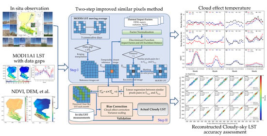
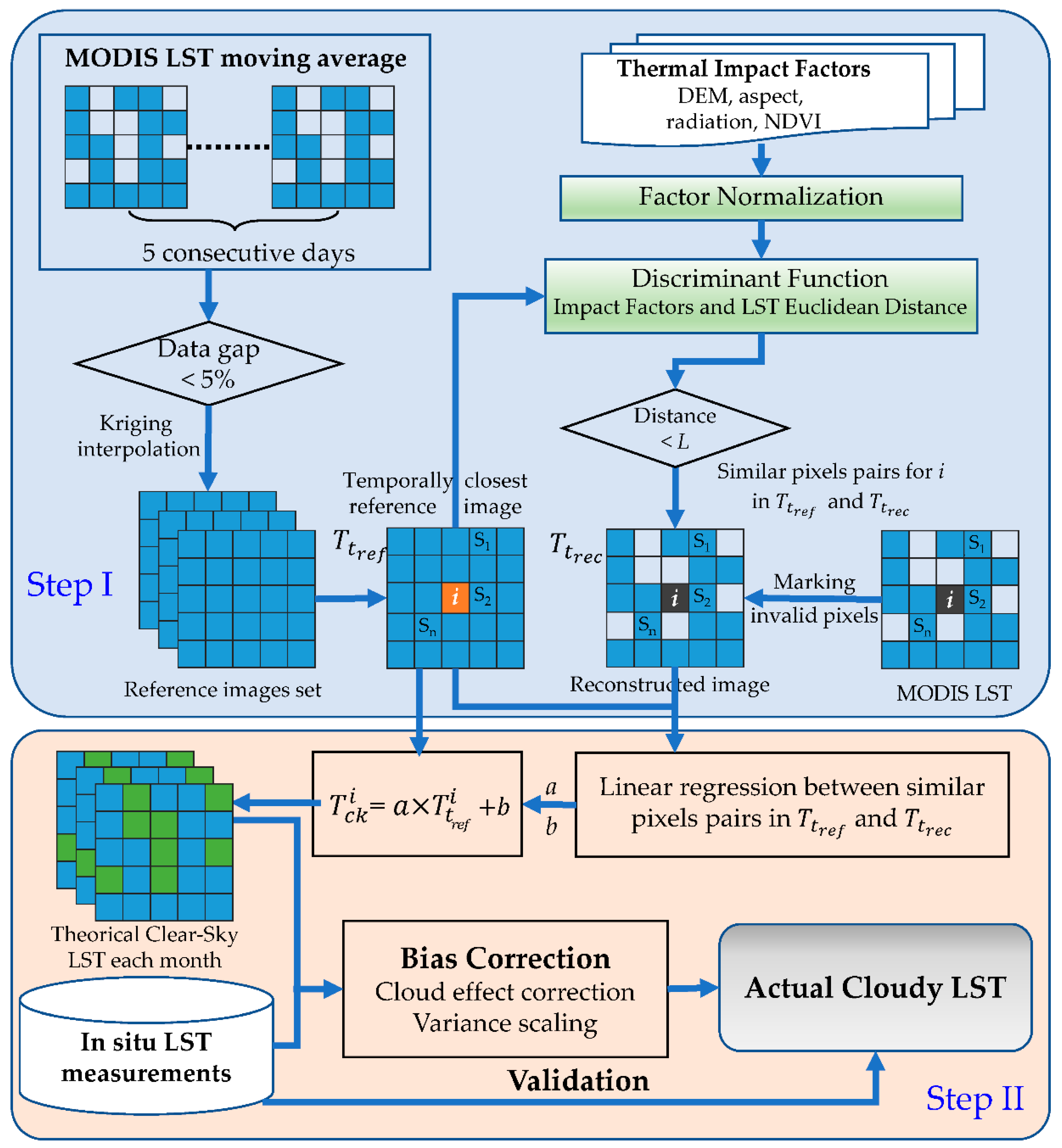
This study intends to develop a two-step framework for the reconstruction of cloudy-sky LST by combining the advantages of the SP method and abundant in situ observation. In situ LST observations from ten automatic weather stations (AWS) during 2013–2018 were used to calculate the cloudiness-induced temperature bias for different land cover types and then to correct the theoretical clear-sky LST. In addition, LST observations performed by all fifteen AWS (including ten AWS for bias correction) during 2013–2018 were used to validate the accuracy of the reconstructed cloudy-sky LST. The new method resolves the instability of the SP method in the reference image selection and maximizes the potential of in situ observations by combining the SP method and a statistical bias correction approach between in situ observations and theoretical clear-sky temperatures.
3. Results and Discussion
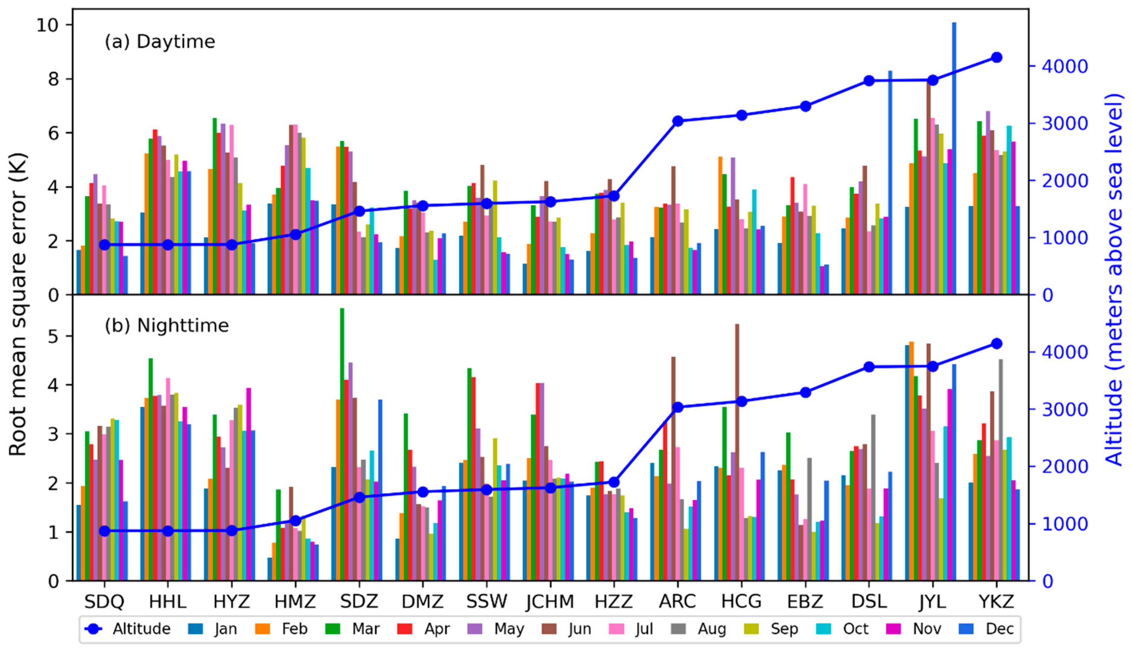
The estimated theoretical clear-sky LST indicates that clouds cool the land surface during the daytime and warms it at nighttime (Terra overpass times,
Figure 6). The response amplitude and trends vary by land surface types (
Figure 7). The TISP method reconstructed cloudy-sky LST was validated using the in situ LST at fifteen stations.
Figure 8 and Table 5 show the verified results for daytime and nighttime.
For the MBE, RMSE, and R2 between the reconstructed cloudy-sky LST and ground measurement LST, the mean MBE of 0.15 K, mean RMSE of 2.91 K, and mean R2 of 0.93 at nighttime are better than daytime (mean MBE = −0.43 K, mean RMSE = 4.41 K, and mean R2 = 0.90). The accuracy is lower in the sparsely vegetated shrub and tree type in the arid region in the daytime.
3.1. Generating the Theoretical Clear-Sky LST
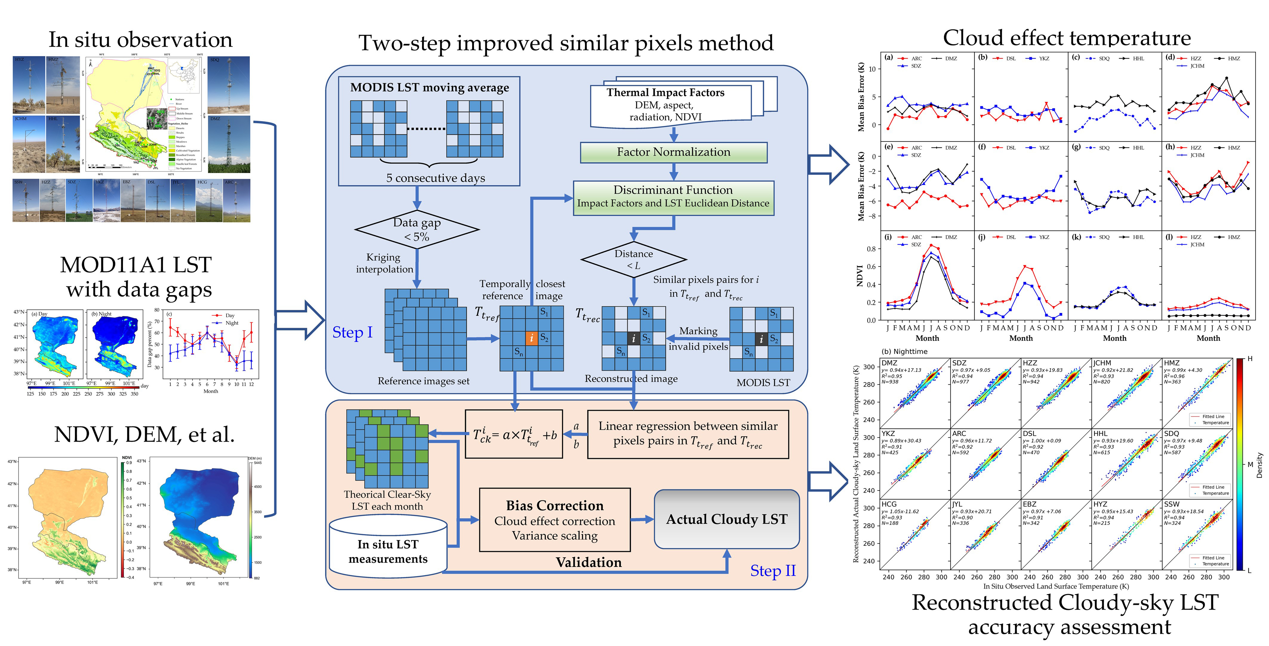
The missing data covered by clouds were estimated using the TISP method in Step I (
Figure 5) to generate theoretical clear-sky LST (
Tck).
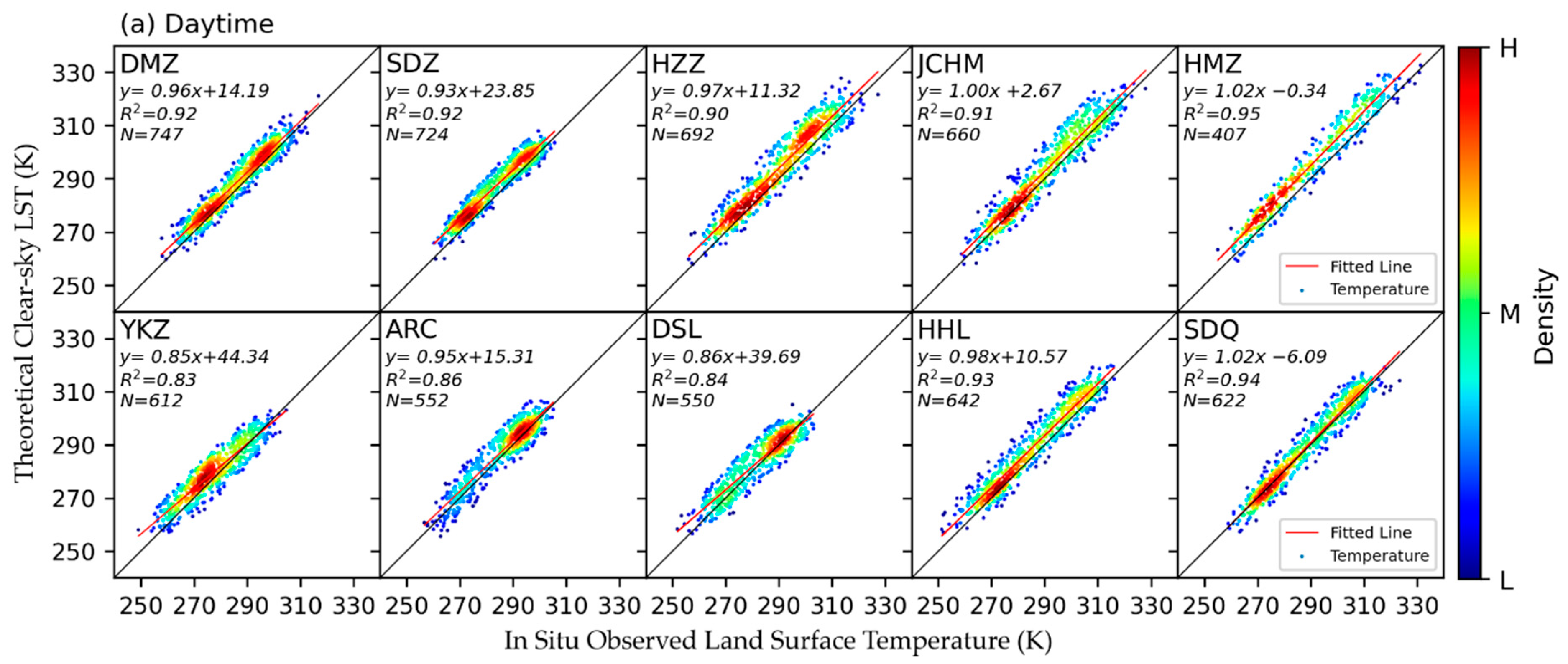
Tck and the in situ LST (
Tin situ) on cloudy days were compared across the ten stations (
Figure 6). Because the
Tin situ measurements compared with the
Tck represent the cloudy-sky condition, the fitted line of the
Tck data at daytime is situated above the 1:1 line (
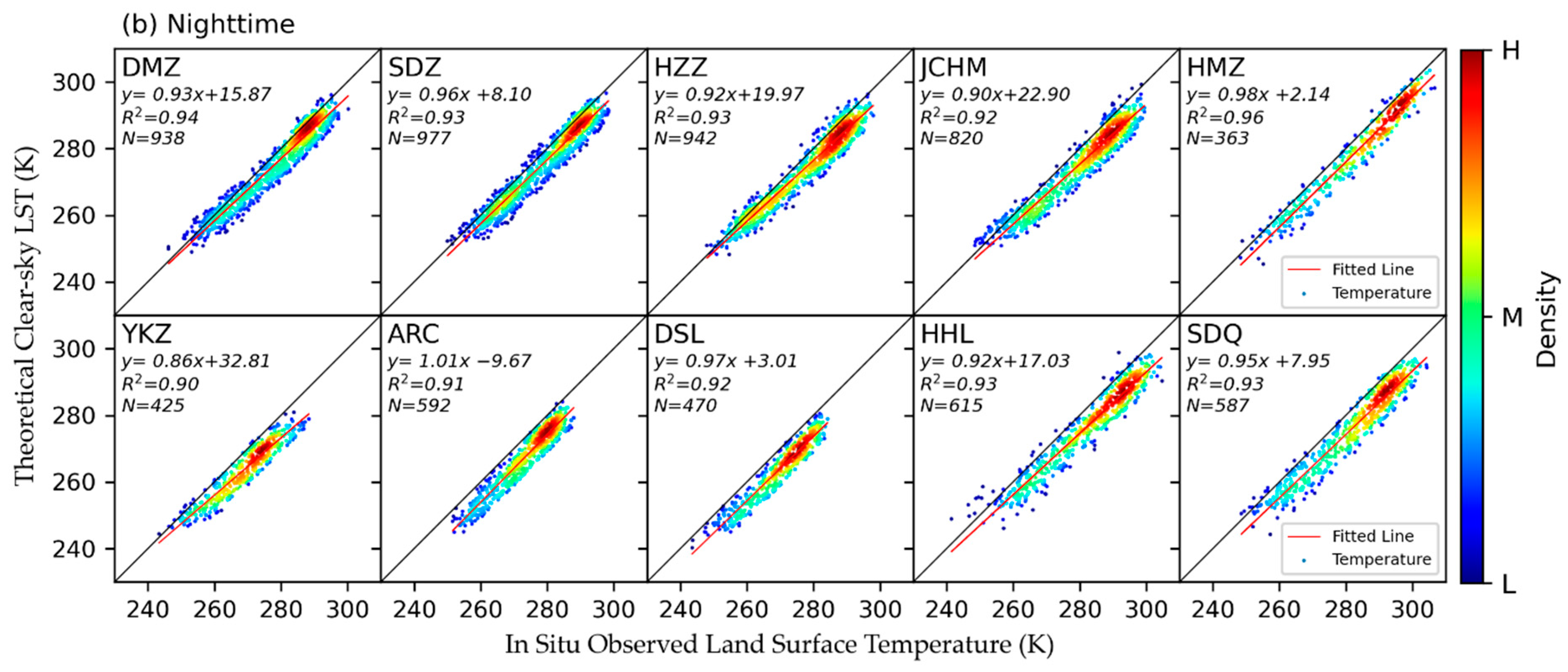
Figure 6a) owing to the cloud cooling effect by decreasing downwelling shortwave radiation. In contrast, the
Tck is lower than the
Tin situ because of the warming effect due to the cloud increased downwelling longwave radiation at nighttime.
The accuracy evaluation statistical metrics for
Tck are shown in
Table 3, which are similar to those shown in
Figure 6. The differences between the
Tck and
Tin situ for cloudy skies vary with time. The comparison of
Tck and
Tin situ on cloudy days results in mean MBE of 2.76 K, mean RMSE of 5.16 K, and mean
R2 of 0.90 at daytime; mean MBE of −4.69 K, mean RMSE of 5.67 K, and mean
R2 of 0.91 at nighttime. There is higher
R2 and MBE between the
Tck and
Tin situ at nighttime than in the daytime.
The above results show that, although it is practicable to estimate the
Tck for cloudy-sky pixels using the TISP method, there is still a systematic bias in the
Tck. Furthermore, the systematic bias between
Tck and
Tin situ is associated with different land cover types [
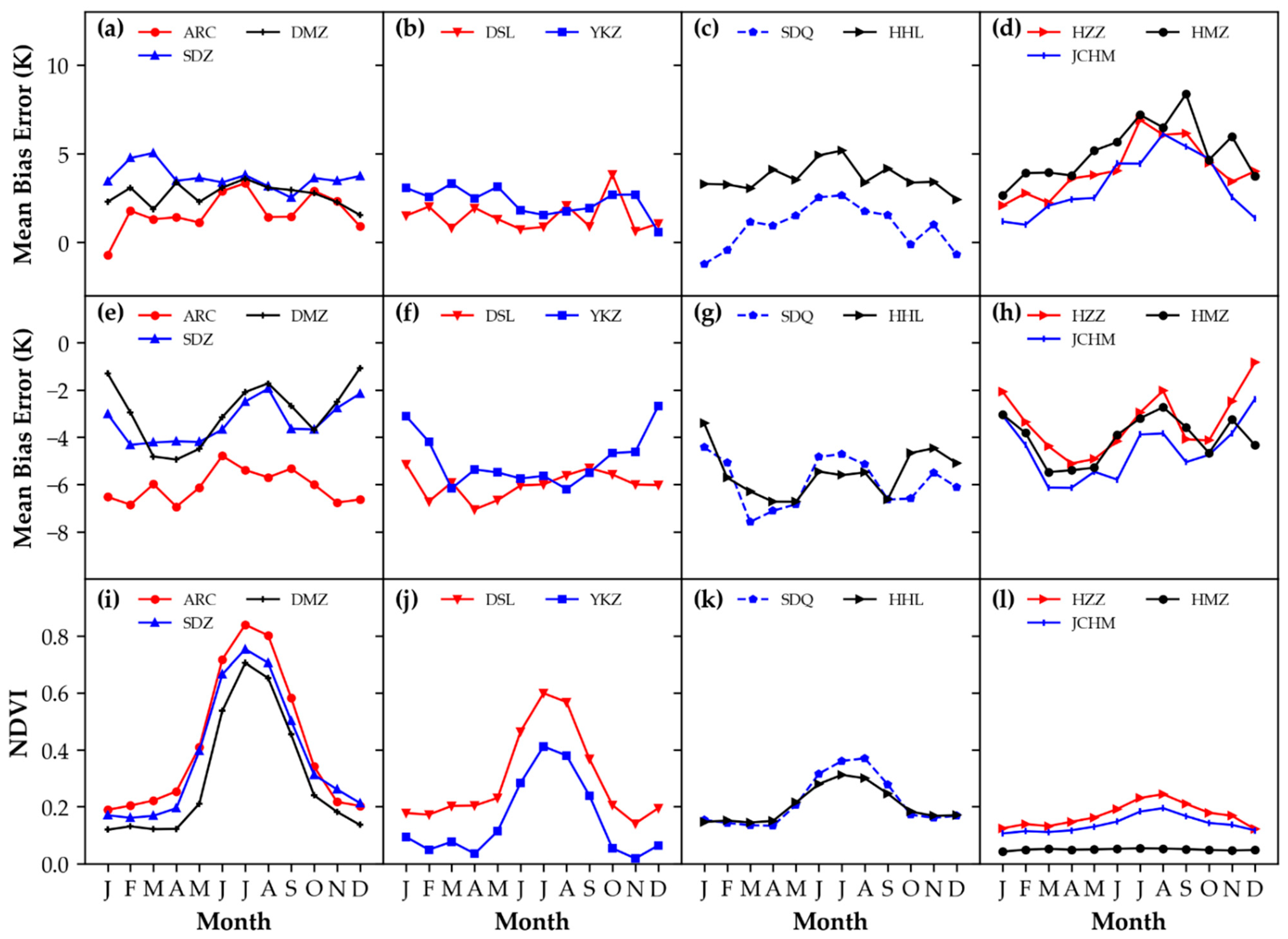
37], which could be a result of how clouds influence the temperature of different surfaces. Therefore, it is essential to quantitatively analyze the cloud effect on LST for different land covers located in different regions. In this research, we classified the land covers into four types according to the summer mean NDVI. According to this classification scheme, ARC (upstream), SDZ, and DMZ (midstream) are high-density vegetation (
Figure 7i); DSL and YKZ (upstream) are medium-density vegetation (
Figure 7j); SDQ and HHL are sparse vegetation (
Figure 7k); HMZ (downstream), JCHM, and HZZ (midstream) is bare land (
Figure 7l).
Figure 7 displays the monthly MBE (
Tck–
Tin situ) of four types of stations at daytime and nighttime, positive MBE indicates a cooling effect of the clouds and negative MBE indicates a warming effect.
Figure 7a, b show that the high and medium-density vegetation stations have similar cloud cooling amplitude and no seasonal trend. The sparse vegetation stations show a moderate seasonal trend, low cooling in winter and moderate cooling in summer with net cooling annually (
Figure 7c); bare land stations show a strong seasonal trend, low cooling in winter and high cooling in summer with net cooling annually (
Figure 7d).
At nighttime, most stations show a net warming effect of clouds, high warming amplitude in spring, moderate in summer, and low in winter. The temperature affected by cloud at most stations showed a monthly “W” shape trend caused by similar cloud cover (
Figure 7e–h); the max warming amplitude of about 7 K appears in spring at the sparse vegetation and bare land sites (
Figure 7g); ARC shows a different trend with a warming amplitude of 5–7 K, a max warming amplitude of 7 K also appears in spring and winter (
Figure 7e).
Figure 7c,g show the daytime and nighttime cloud effects temperature amplitude at sparse vegetation stations. They have the same seasonal trend in daytime and nighttime, but HHL has a stronger cooling effect than SDQ in the daytime. The sparse vegetation stations have a max cooling amplitude of about 5 K in summer and a warming amplitude of about 8 K in spring.
Figure 7d and h show the daytime and nighttime temperature changes caused by cloud cover at bare land stations (HZZ, JCHM midstream, HMZ downstream). These stations have the same trend of cloud effect amplitude on the temperature in the daytime and nighttime. The max cooling amplitude of about 8 K appears in summer and warming amplitude of about 6 K in spring.
Most of the subfigures in
Figure 7 show the same trend and similar amplitude. The yearly cloud effect temperature statistics are shown in
Table 4. At bare land sites, located in the middle and downstream, the temperature change trends caused by cloud cover are seasonal and very similar between stations, with a cooling amplitude of 4.14 K in the daytime and warming of 3.99 K at nighttime. For dense vegetation, the temperature change trends have a small seasonality and are very similar across stations during the daytime. Therefore, LST can be corrected for cloud effects in each pixel by using the bias correction of stations grouped by vegetation density class.
3.2. Validation
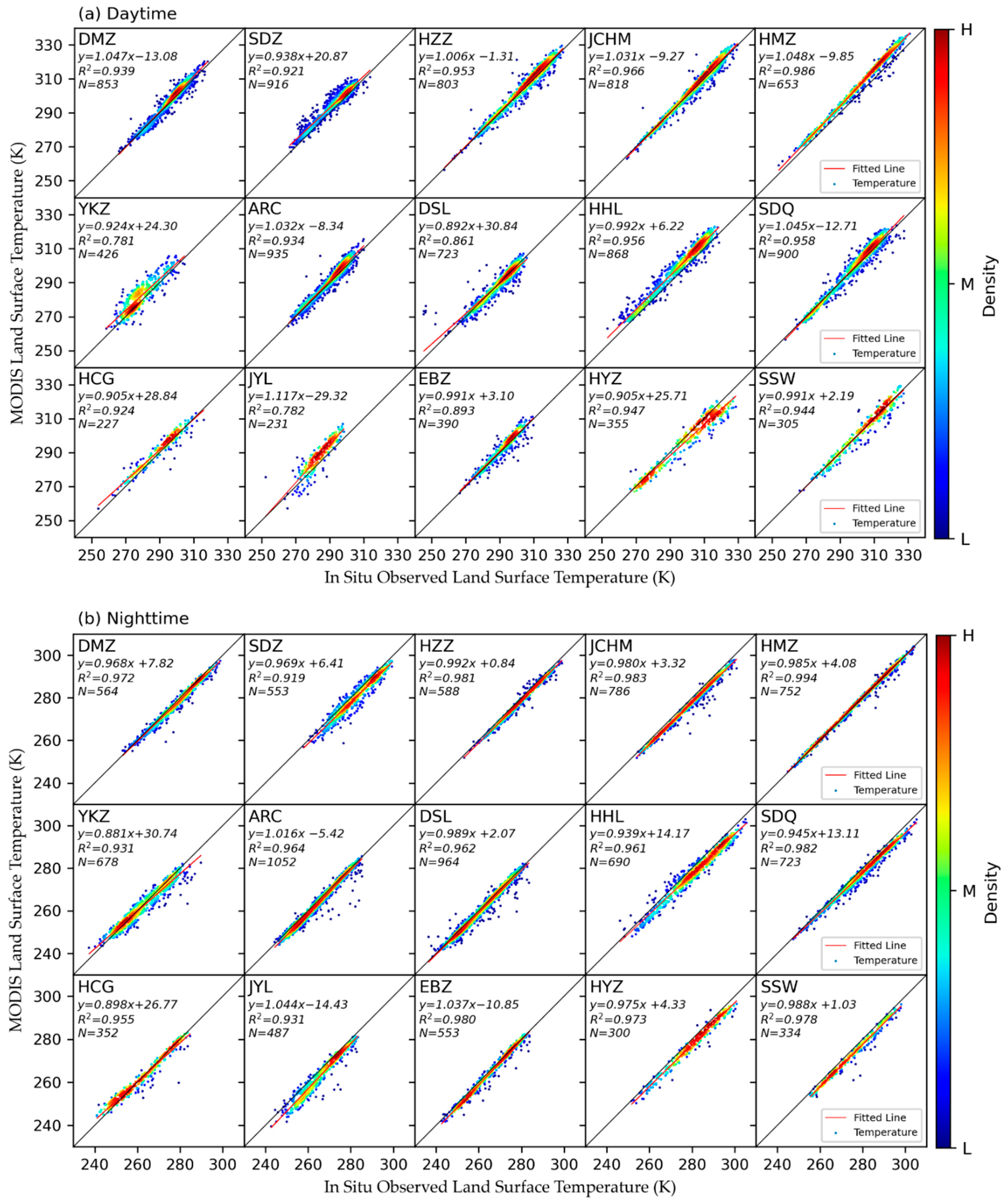
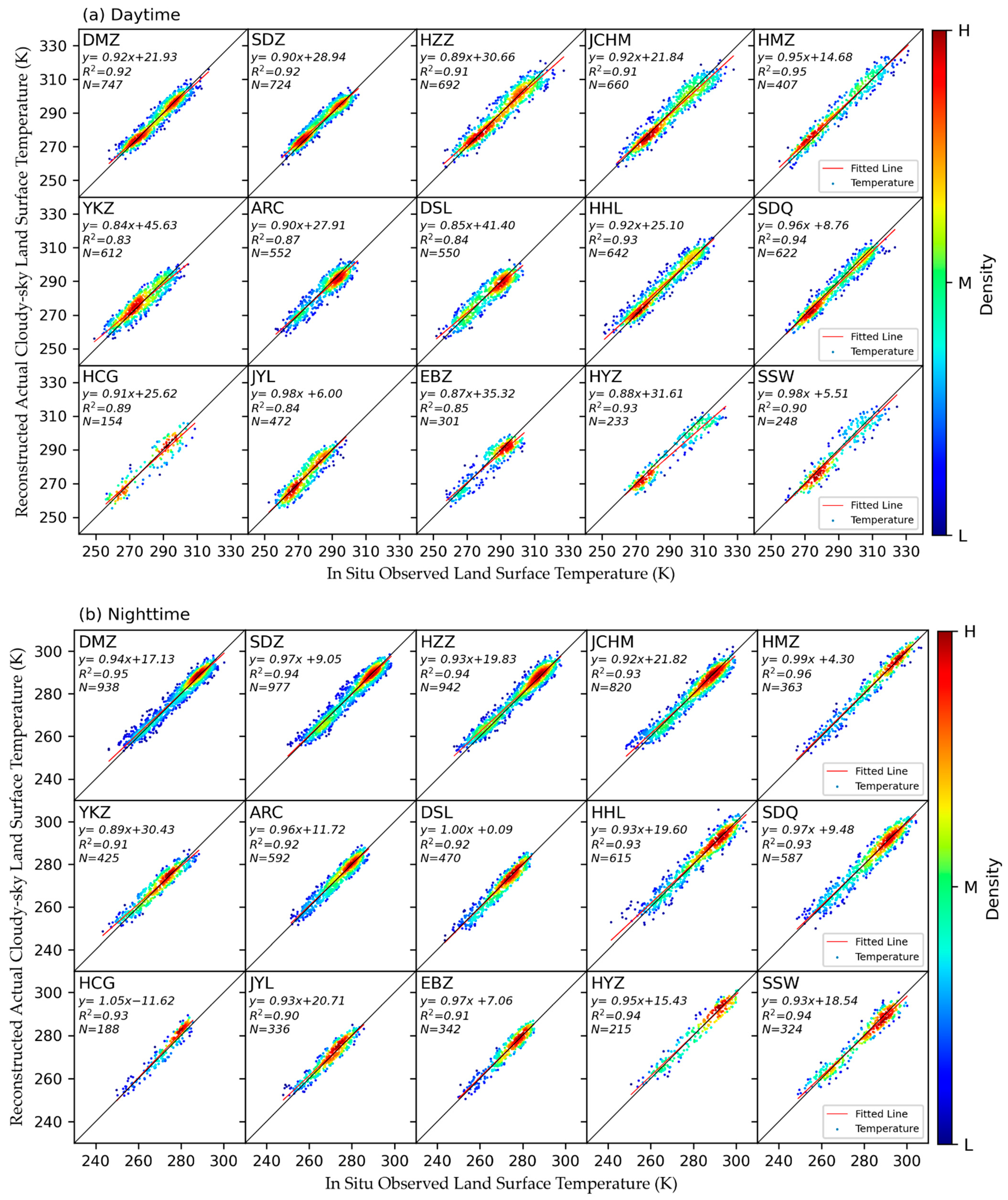
To verify the accuracy of the new TISP framework, the corrected actual cloudy-sky LST (Tcd) was validated with the data from the fifteen stations during 2013–2018. To minimize the biases caused by time mismatch, only the in situ LST observations matching the Terra overpass times within the closest half hour were chosen.
The validation scatters density plots are shown in
Figure 8a (daytime) and
Figure 8b (nighttime). The plots indicate that most of the scatter points between
Tcd and
Tin situ are concentrated around the 1:1 line. Moreover, the
Tcd at nighttime shows greater agreement with the in situ LST measurement than at daytime.
Table 5 shows the statistical metrics (MBE, RMSE, and
R2) for each station. The mean statistical metrics for all stations, ten bias correction stations, and five independent stations are shown in
Table 6. The validation accuracy of all stations indicates that the
Tcd have mean MBE <0.50 K (−0.43 K at daytime, 0.15 K at nighttime), mean RMSE of 4.41 K, and
R2 of 0.90 at daytime, and have mean RMSE of 2.91 K, and
R2 of 0.93 at nighttime. The accuracy of five independent stations have mean MBE of −1.32 K, mean RMSE of 4.86 K, and
R2 of 0.88 at daytime, and have mean MBE of 0.26 K, mean RMSE of 2.79 K, and
R2 of 0.92 at nighttime, slightly lower than the result of all stations.
Figure 8a compares
Tcd against
Tin situ in the daytime. Overall, most of the
Tcd show an excellent agreement with the
Tin situ. The MBE of all stations is between ±1.5 K. For five independent stations, MBE ranged from −3.56 K to −0.08 K and
R2 ranged from 0.84 to 0.93. The accuracy of the
Tcd at the sparse vegetation stations (HHL, SDQ, and HYZ) are lower than others. This may be due to three reasons: (1) The MODIS LST product has poor accuracy in arid areas and few outliers with large errors due to undetected clouds. It may cause similar pixels generated by the TISP method to have large uncertainty, which directly impacts the accuracy of
Tck. (2) There is uncertainty in the cloud effect temperature term estimation in these two stations. Although they belong to the sparse vegetation type (the stations have similar NDVI), the land surface of HHL and HYZ is mixed with sand,
Populus euphratica, and
Tamarix, thus the tree shadows increase the heterogeneity in the regional temperature [
62], while SDQ is mixed with sand and
Tamarix, resulting in a more homogeneous land surface than HHL. This directly impacts the accuracy of the cloud effect temperature of this land cover type (
Figure 7c). (3) These three stations are very close to each other (
Figure 1), resulting in a big bias from large viewing angles.
Figure 8b is the validation result at nighttime. For all stations, MBE ranges from −0.37 to 0.92 K, with an average MBE of 0.15 K; RMSE ranges from 2.49 to 3.47 K, with an average RMSE of 2.91 K;
R2 ranges from 0.91 to 0.96 (
Table 5), with a mean
R2 of 0.93.
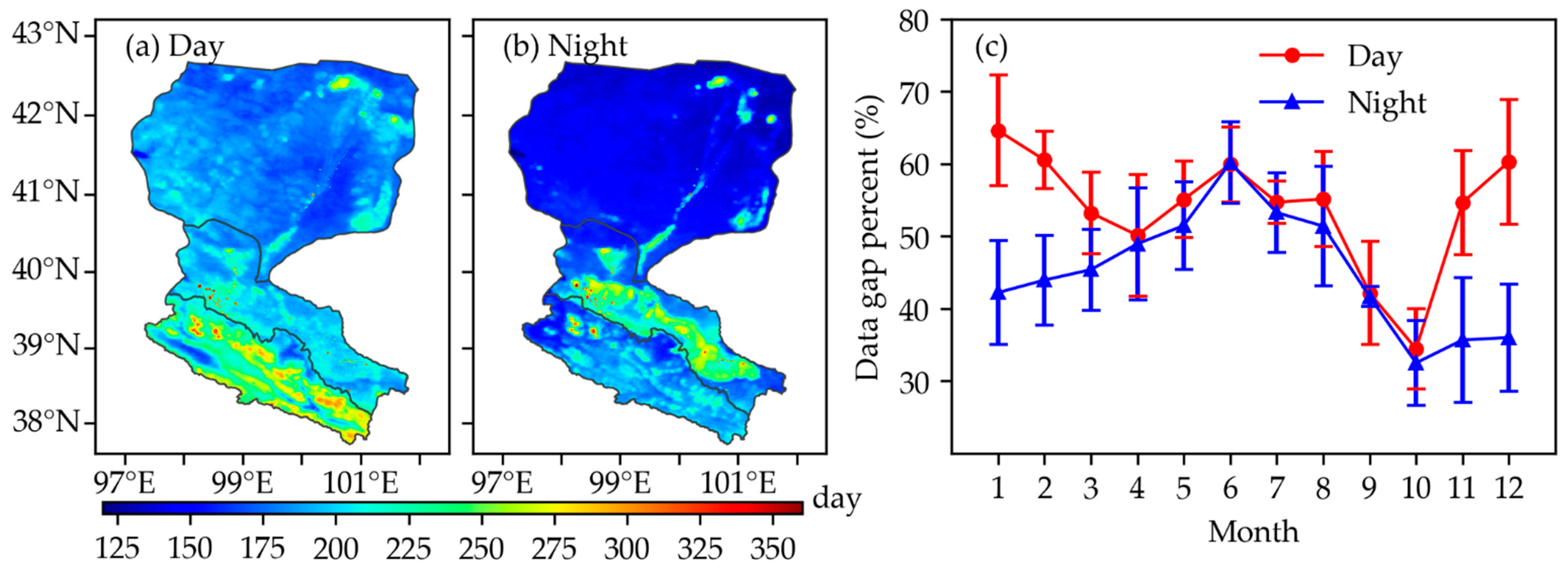
Figure 3 and
Table 5 show the evaluation of MODIS LST for daytime and nighttime. The validation accuracy of the MODIS LST product has an average MBE of 1.32 K (−1.58 K), average RMSE of 3.96 K (2.64 K), and average
R2 of 0.93 (0.95) at daytime (nighttime).
Overall, the accuracy of the TISP method at all stations is generally comparable to the accuracy of the valid MODIS data. The corrected Tcd at most stations has better agreement with the Tin situ at nighttime than daytime. The result shows that the TISP method is dependable for most land cover types in HRB. The in situ LST observation at Terra overpass time in the cloudy sky varied from 250 K (240 K) to 330 K (320 K) during 2013–2018. This temperature range can represent HRB’s temperature in cloudy skies. This means that the TISP method is reliable for basin-wide applications in the HRB.
3.3. An Experiment for Testing the Accuracy of the Tck
In order to verify the accuracy of the
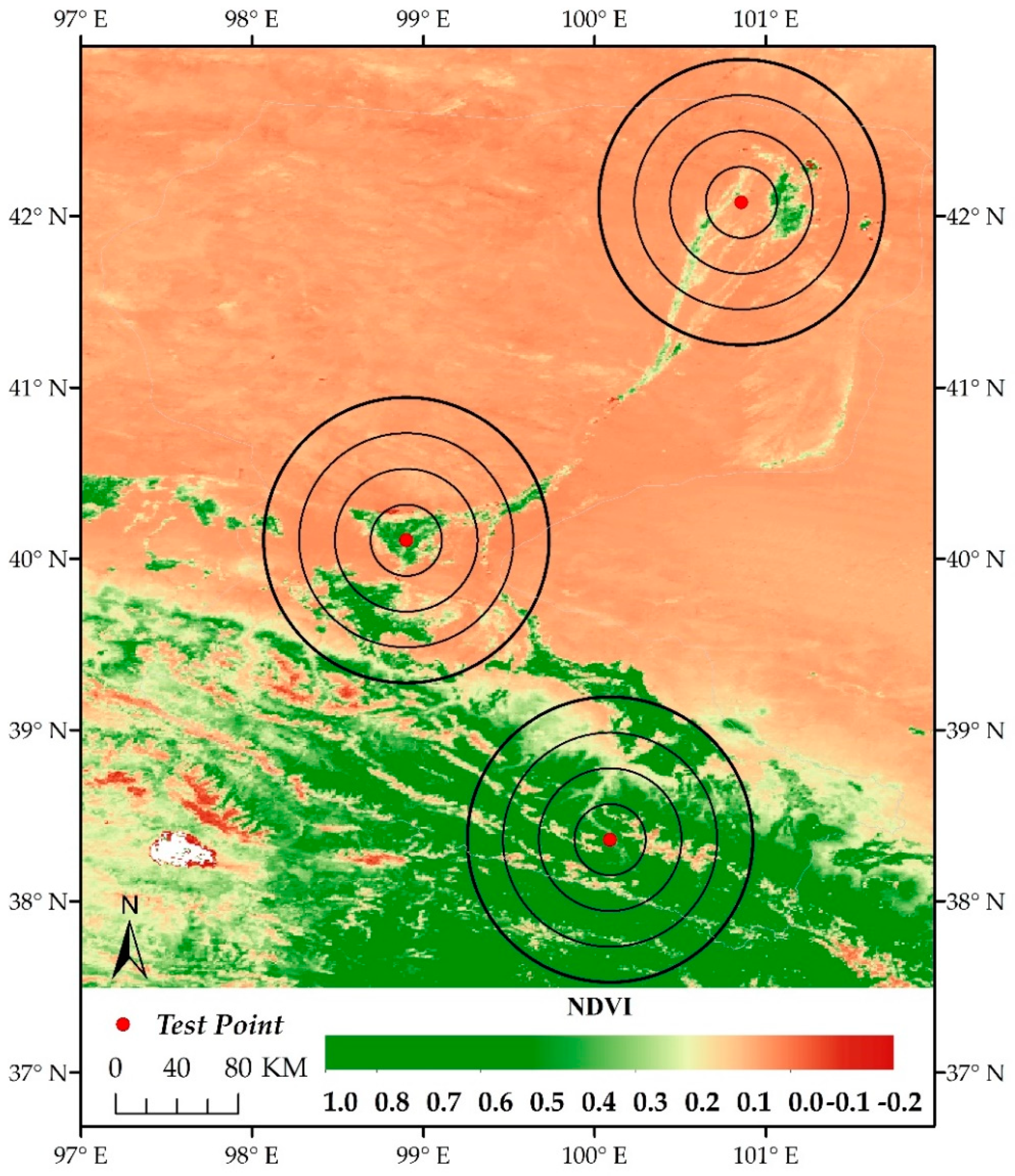
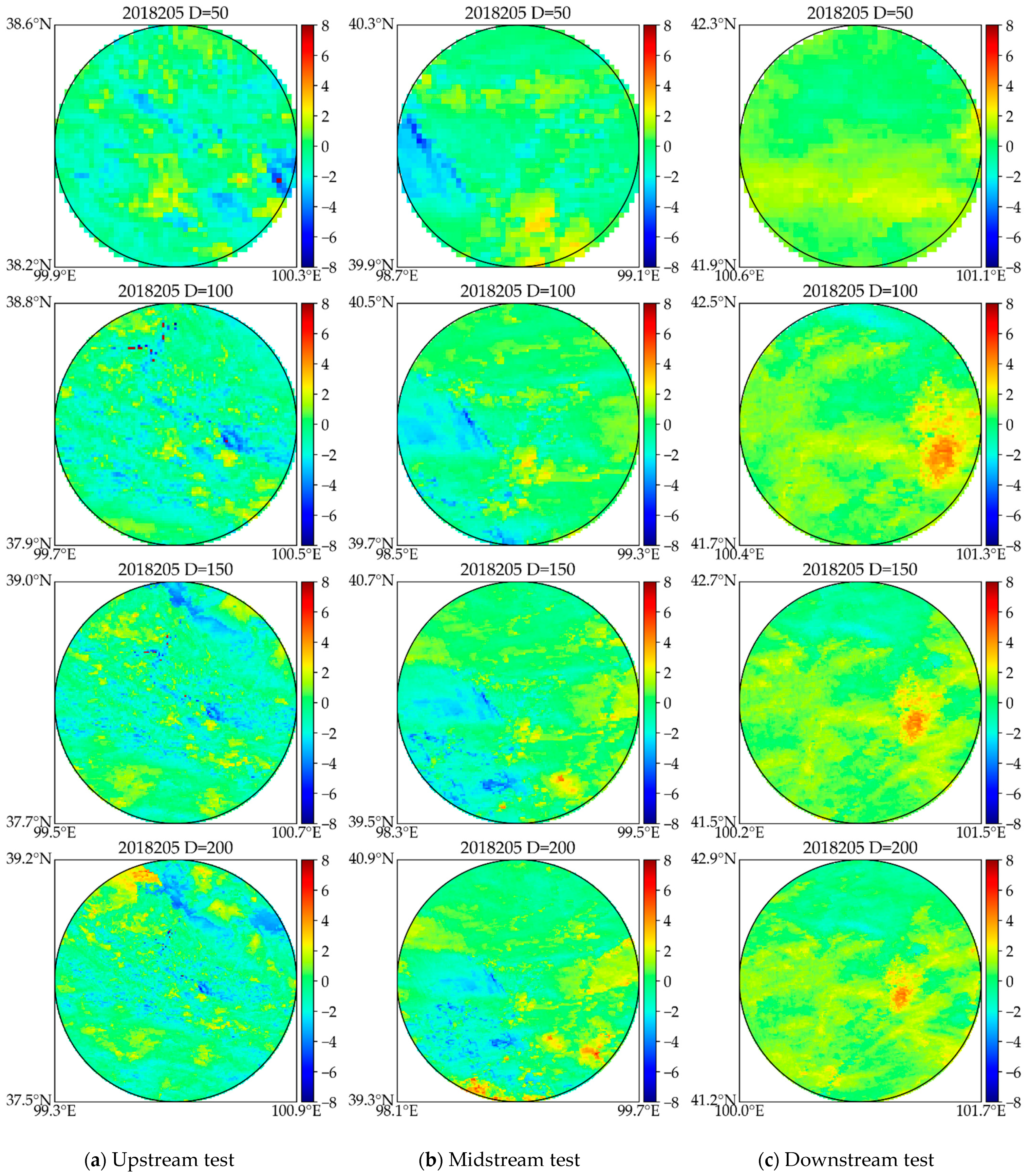
Tck, a numerical simulation experiment was designed for clear-sky MODIS LST images. For the experiment, two images of daytime and nighttime LST (data gaps <5%) from the MOD11A1 LST product were selected for day 205 of 2018. Then, the original MODIS LSTs were masked with four circular areas with diameters of 50, 100, 150, and 200 km in three experiment regions (
Figure 9). The four black circles with diameters (D) of 50, 100, 150, 200 km centered on each red dot represent the simulated cloud cover area, which was then reconstructed. The three typical experiment areas are located in a relatively dense vegetation cover area upstream (upstream test), medium vegetation cover region midstream (midstream test), and low vegetation cover area downstream of HRB (downstream test). Upstream test is the most complicated site because it has relatively less vegetation heterogeneity but large elevation changes.
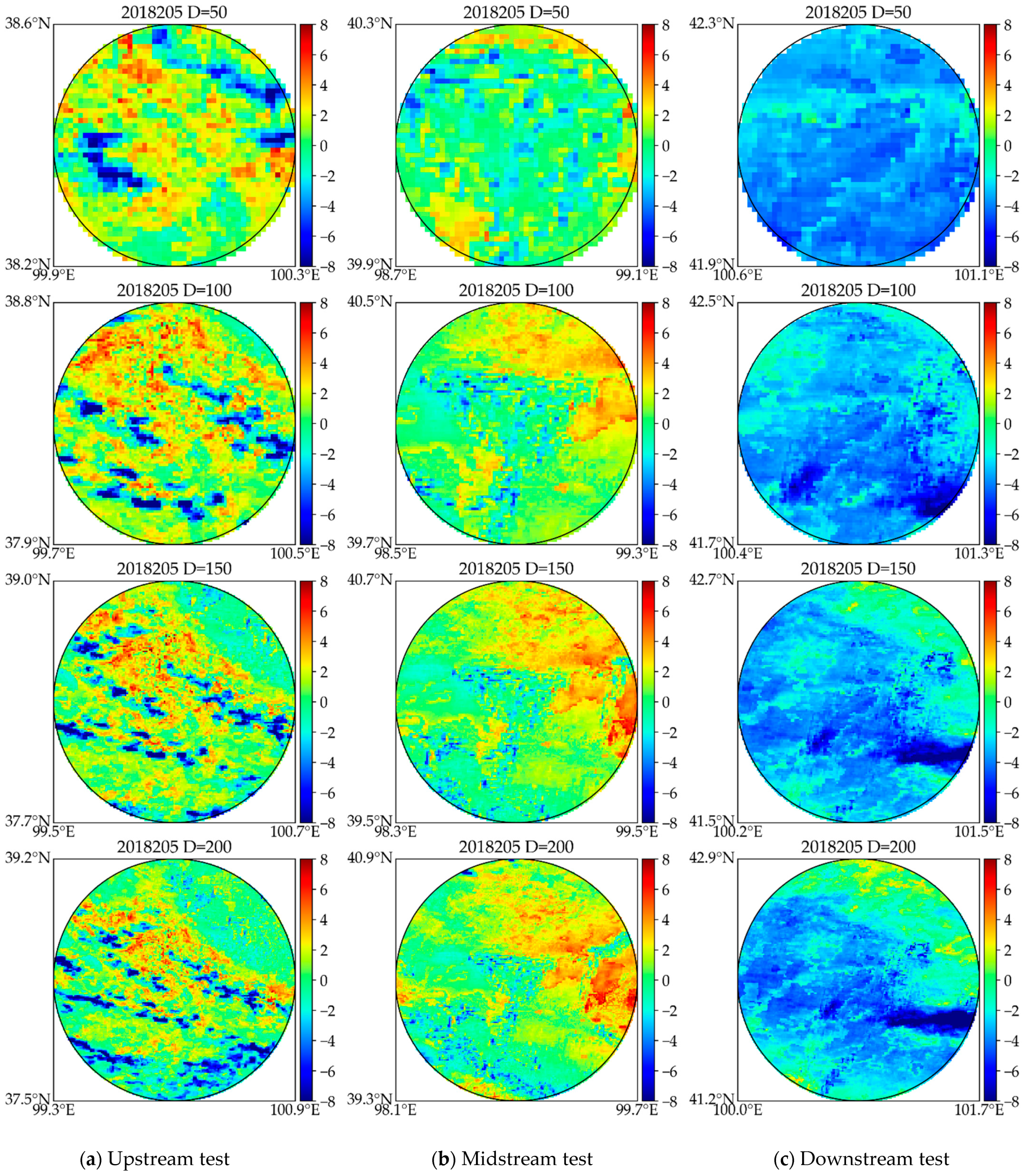
The simulated cloud cover areas in the circles with different diameters were reconstructed using the TISP method, and the difference between the reconstructed
Tck and MODIS LST was calculated at each experiment area (
Figure 10 and
Figure 11). The result indicates that the TISP method has better performance in the upstream and midstream and the difference image was very close to 0 K (
Figure 12). The downstream test result (
Figure 10c and
Figure 11c) shows that the TISP method may overestimate at daytime and underestimate at nighttime. Therefore, the TISP method is more accurate in areas of dense vegetation than bare land, because MODIS LST has lower accuracy in bare land, especially in the daytime. At nighttime, all regions have similar accuracy and better than daytime because the land surface becomes more homogeneous during nighttime. For each test region, the difference between MODIS LST and
Tck displays similar results among different diameters.
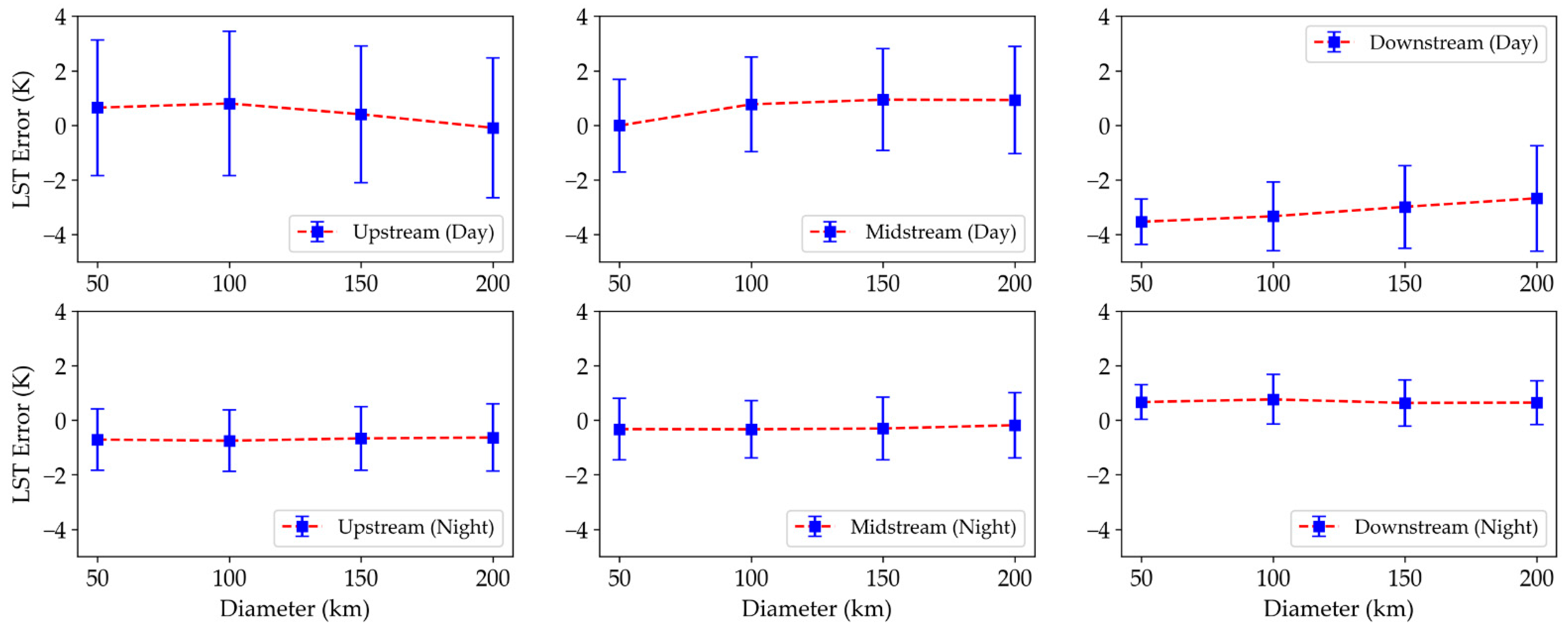
To quantitatively analyze the accuracy of the TISP method for
Tck generation, the MBE and standard deviation (STD) between MODIS LST and
Tck were calculated (
Figure 12). Most MBE of the
Tck is concentrated in ±1 K. The range of MBE in the daytime is slightly decreased from 0.79 K to −0.10 K upstream, increased from −0.01 to 0.94 K midstream, decreased from −3.53 K to −2.65 K downstream. At nighttime, the range of MBE is smaller and more stable than daytime, ranging from −0.71 to −0.63 K upstream, from −0.33 to −0.18 K midstream, from 0.63 to 0.76 K downstream.
The average STD for each test area is less than 3 K in the daytime and less than 1.5 K at nighttime (
Figure 12). At daytime, STD ranges from 2.47 to 2.71 K upstream, from 1.69 to 1.96 K midstream, and from 0.83 K to 1.87 K downstream. The STD remains relatively stable in the three experiment regions with D = 50 km to 150 km. At nighttime, STD changes from 1.12 K to 1.23 K upstream, from 1.04 K to 1.19 K midstream, and from 0.63 K to 0.91 K downstream. The STDs at nighttime are more stable than at daytime.
In most experiments, the accuracy of the TISP method is similar in different simulated cloud cover areas because, for a certain area, the regressed function derived from similar pixels between the reconstructed and reference image are relatively stable. Moreover,
Figure 10,
Figure 11 and
Figure 12 indicate that the downstream test has the greatest MBE among all tests, while the upstream and midstream tests show smaller LST bias. For the cloud cover area, the spatial structure of the regional LST distribution has a greater influence on the TISP method than the area of cloud cover area.
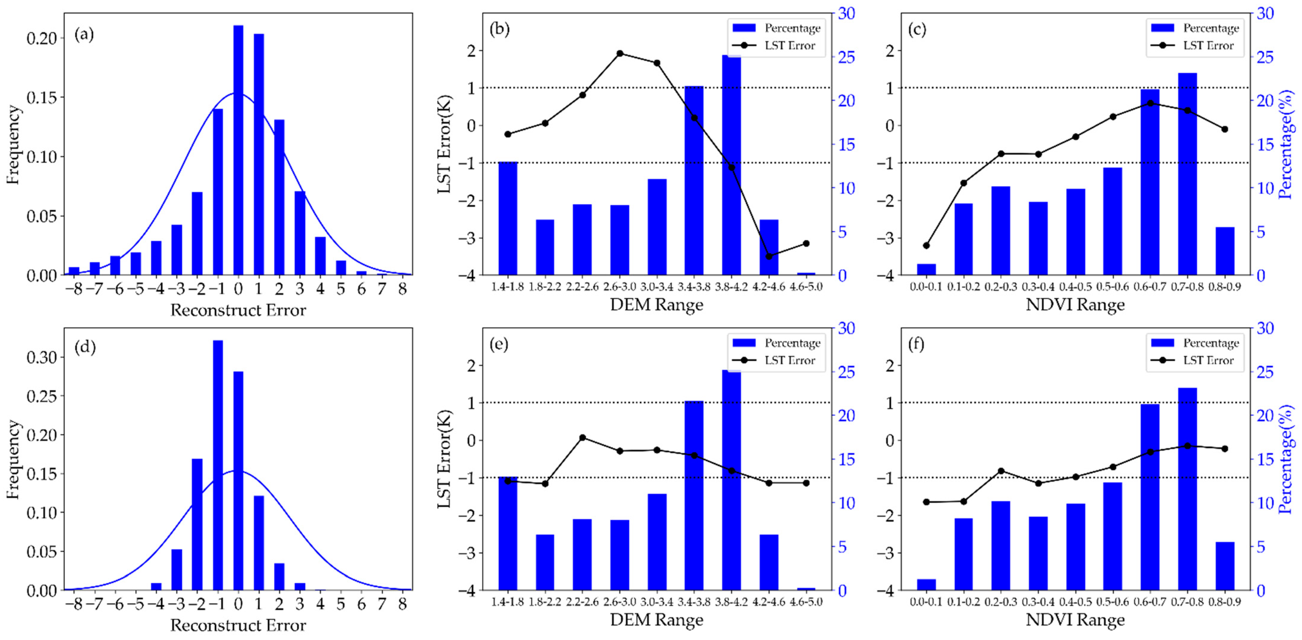
To test the topographic impact of the TISP method, the simulated cloud cover area with 200 km diameter upstream was selected to compare the MBE with the DEM and NDVI range at daytime and nighttime. The distribution histograms of MBE for the difference image (original MODIS LST minus
Tck) are shown in
Figure 13a,d for day and night, respectively. The MBE distribution histogram shows that the average biases of most test areas are close to 0 K and are concentrated in ±1 K, although there were few larger bias values. The percentage of bias in the range ±1 K is 54.6% during daytime and 72.4% at nighttime. Therefore, the TISP method yields slightly higher accuracy with nighttime than daytime data.
Figure 13b,e show the MBE within different classes of DEM in daytime and nighttime. From
Figure 13b,e, the MBE is higher at high elevations (>4200 m), but the percent is less than 5%.
Figure 13c,f shows the MBE within different classes of NDVI. From
Figure 13c,f, the MBE is higher in the lower NDVI (<0.1), but the percent is <5%. Therefore, judging from the overall accuracy and the effect of the DEM and NDVI, the TISP reconstruction method is sensitive to the DEM factor at high elevations and the NDVI factor at lower NDVI values at daytime.
3.4. Research Limitations
The TISP method proposed in this paper provides a new framework that takes full advantage of ground-based observation. While it shows good accuracy, TISP also still presents some limitations.
The impact factors used to select similar pixels in TISP include DEM, slope, aspect, NDVI, and theoretical radiation. Although NDVI represents, to some extent, the state of the land cover, it may cause a similar pixel selection algorithm to misclassify low NDVI areas. Bare land has the largest area in HRB and is widely distributed, including bare rock, the Gobi Desert, sand desert, saline land, etc. It is difficult to discriminate among these bare land types due to their low NDVI values; therefore, to improve the accuracy of the TISP method on bare land, we need to further develop a long time series land cover product that includes more refined land cover types.
The original MODIS LST data presents some anomalies (
Figure 3a) caused by undetected clouds [
53,
69]. Although some of the anomalies can be eliminated through quality control, they cannot be completely eliminated, affecting reference image generation and model construction. Therefore, more attention needs to be paid to identifying cloud-contaminated pixels in the MODIS LST product before performing LST reconstruction.
On the other hand, two empirical parameters may affect the accuracy of the TISP method, one is the number of consecutive days, and another is the data gaps rate threshold. Setting a larger number of consecutive days can increase the amount of valid data in the image. However, it can also lead to a weakening of the correlation between similar pixels in the reference image. Too small of a data gap rate threshold may result in a small number of reference images, consequently the large interval between the reference image and reconstructed image.
The impact of cloud type on LST for different land covers needs to be studied further. In this paper, the theoretical clear-sky LST was compared with ground-based observations and found that the effect of clouds on LST varies seasonally and with land cover. At night, the warming effect of clouds on LST is higher in spring and autumn under most vegetation types, which is mainly due to the different cloud types in these seasons. The spatial distribution and temporal variation characteristics of cloud types in HRB were not discussed in depth in this paper. Research on the influence of cloud types on LST should be strengthened in future studies.
For regions with adequate and typical ground-based observations, the TISP method is applicable to other thermal remote sensing sensors with short satellite revisit cycles, which can provide a sufficient number of validation data required for bias correction.
The TISP bias correction requires in situ LST measurements to construct the cloud effect temperature term. Therefore, it cannot be directly applied to regions without in situ measurements. However, the bias correction can be improved by calculating the cloud effect temperature term from the comparison between calibrated land skin temperature of reanalysis data [
39] against the theoretical clear sky LST.
In recent years, all-weather LST generation methods have evolved from single data source to multi-source data fusions. Future research will focus on combining the advantages of TIR and microwave LST from polar and geostationary satellites, ground-based observations, and model output data to derive a global, gap-free LST product.
4. Conclusions
In this research, we proposed the TISP method to reconstruct actual cloudy-sky LST for MOD11A1 data. First, the theoretical clear-sky land surface temperature was estimated based on the improved similar pixel algorithm. Then, bias correction for the theoretical clear-sky land surface temperature used the cloud effect temperature component calculated from the statistical relation between in situ LST measurements and theoretical clear-sky land surface temperature.
The estimated theoretical clear-sky temperature indicated that clouds cool/warm the land surface during day/night in HRB, China. For bare land located mid- and downstream, the temperature change trends caused by cloud cover have obvious seasonality and similarity; cloudiness causes an approximate reduction of the yearly mean value of 4.14 K, ranging from 3.18 to 5.12 K during the day, while an increase of the yearly mean value of 3.99 K, ranging from 3.38 to 4.55 K at night on a monthly average was observed. For dense vegetation, temperature change trends have small seasonality and are very similar across stations during the day.
This TISP method and MODIS LST product had been validated against in situ observation of LST at 15 stations during 2013–2018, and the accuracy assessment of the reconstructed actual cloudy-sky LST at daytime shows that MBEs are between ±1.5 K, except for one station of −3.56 K, RMSEs of 3.40–5.66 K, and
R2 of 0.83–0.95; at nighttime, the accuracy shows that MBEs are between ±1.0 K, RMSEs of 2.57–3.47 K, and
R2 of 0.90–0.96. Overall, the accuracy assessment of the cloudy-sky LST with results in mean MBE of −0.43/0.15 K, mean RMSE of 4.41/2.91 K, and
R2 of 0.90/0.93 at daytime/nighttime, which is consistent with the recently published studies [
37,
41] and MODIS LST product accuracy with a mean MBE of 1.32/−1.58 K, and a mean RMSE of 3.96/2.64 K.
Overall, the developed method maximizes the potential use of MODIS LST data over cloud cover effect on temperature with in situ observations, and can successfully reconstruct cloudy pixels under all-sky conditions. The validation and experimental results show that for most land surface types the TISP method has high accuracy, except over sparse vegetation types. Although there is still uncertainty in the TISP method, this study proposed an effective and very simple guideline for MODIS cloudy-sky LST reconstruction at the basin scale where abundant ground-based measurements for most land surface types are available. In a future study, the new fusion framework will be developed to generate a long time series of LST datasets by taking advantage of additional thermal infrared and microwave remote sensing data, model outputs, and in situ observation.


