Article

Predicting Height to Crown Base of Larix olgensis in Northeast China Using UAV-LiDAR Data and Nonlinear Mixed Effects Models

Key Laboratory of Sustainable Forest Ecosystem Management-Ministry of Education, School of Forestry, Northeast Forestry University, Harbin 150040, China
*
Author to whom correspondence should be addressed.
These authors contributed equally.
Submission received: 29 March 2021 / Revised: 25 April 2021 / Accepted: 6 May 2021 / Published: 8 May 2021
(This article belongs to the Section Forest Remote Sensing)

Abstract

:
As a core content of forest management, the height to crown base (HCB) model can provide a theoretical basis for the study of forest growth and yield. In this study, 8364 trees of Larix olgensis within 118 sample plots from 11 sites were measured to establish a two-level nonlinear mixed effect (NLME) HCB model. All predictors were derived from an unmanned aerial vehicle light detection and ranging (UAV-LiDAR) laser scanning system, which is reliable for extensive forest measurement. The effects of the different individual trees, stand factors, and their combinations on the HCB were analyzed, and the leave-one-site-out cross-validation was utilized for model validation. The results showed that the NLME model significantly improved the prediction accuracy compared to the base model, with a mean absolute error and relative mean absolute error of 0.89% and 9.71%, respectively. In addition, both site-level and plot-level sampling strategies were simulated for NLME model calibration. According to different prediction scale and accuracy requirements, selecting 15 trees randomly per site or selecting the three largest trees and three medium-size trees per plot was considered the most favorable option, especially when both investigations cost and the model’s accuracy are primarily considered. The newly established HCB model will provide valuable tools to effectively utilize the UAV-LiDAR data for facilitating decision making in larch plantations management.

Graphical Abstract

1. Introduction

The forest biome is valuable for providing abundant wood resources, protecting wildlife habitats, storing a high amount of carbon, regulating micro- and macro-climates, and possessing other numerous ecological functions. It also plays a vital role in the terrestrial ecosystem, in which its fluctuation highly affects the terrestrial biosphere and other surface processes [1,2]. Traditionally, forest resource inventory relies on field sample measurements by collecting and summarizing the tree-level attributes within a designated sampling area through tree-by-tree measurements. Ground-based forest inventory has a high value of precision, consequently needing an immense amount of manpower, material resources, and time [3]. Hence, delivering a prompt forest inventory becomes a problematical obstacle, specifically for the inventory of an extensive forest area [4].
The continuous development of remote sensing technology has brought a promising solution to punctuality and the high-spatial limitation, providing a breakthrough for highly efficient forest inventory [5,6]. Optical remote sensing data has achieved effective results in large spatial extents for stand age identification, volume estimation, and biomass mapping [7,8]. Nevertheless, the optical sensors carried by this passive remote sensing platform may have serious signal saturation dilemmas, leading to the deviation of some forestry parameter extraction results [9]. As a burgeoning active remote sensing technology, airborne light detection and ranging (LiDAR) can provide precise measurements of vertical forest structure. Combined with the ground-based sample data, LiDAR data can obtain more accurate distribution characteristics of forest types and a wider range of three-dimensional spatial structures. There is great potential in estimating forest inventory parameters by analyzing the forest structure dynamics through multi-temporal remote sensing data series [10,11]. Various studies have demonstrated that airborne LiDAR has a special benefit in forest fire behavior prediction, canopy structure extraction, volume and biomass estimation, and other forest attributes and ecosystem structure measurement, in which the accuracy is beyond the reach of its traditional counterparts [12,13,14,15].
For the past few years, with the rapid development of unmanned aerial vehicle light detection and ranging (UAV-LiDAR) remote sensing technology, the research on estimating stand structure parameters by UAV-LiDAR is increasing gradually [16,17]. Compared to the conventional airborne data, the UAV-LiDAR has quite a few advantages, such as lower data acquisition cost, higher pulse sampling density, simpler operational procedure, and higher flight route flexibility [18,19]. Hence, it is gradually becoming a powerful tool for 3D forest mapping and convincingly appears as a low-cost remote sensing alternative to airborne and satellite platforms [20,21]. The high-density point clouds UAV-LiDAR system can obtain relatively high precision for tree height and crown structure measurement [22]. The high spatial resolution of UAV-LiDAR provides high-precision single-tree segmentation which leads to stronger data availability and a more accurate algorithm [23,24]. At present, the extraction of tree height and crown information is crucial for the single-tree-based forest inventory [25,26].
Crown is a crucial component of an individual tree that facilitates a material exchange and energy transformation between the forest and environment, greatly determining trees’ vegetative space, such as sunlight, photosynthesis, and water utilization [27]. The height to crown base (HCB) of a standing tree is defined as the distance from the first living branch at the crown’s base to the ground position [28]. HCB reflects the crown’s vertical structure and is closely related to the number of foliage [29]. As an essential indicator of an individual tree’s crown characteristics, HCB not only determines the yield, productivity, and growth vigor of an individual tree [30] but also reflects the competition status of a tree within the stand along with other non-natural factors [31,32,33]. HCB is also a decisive variable in the stand growth and yield model and plays a pivotal role in the crown width model [34,35], crown shape model [36], biomass model [37], and fire behavior model [38]. However, in the actual measurement of HCB, especially in stands with large canopy density and complex forest conditions, the measurement accuracy is poor, and thus the efficiency is low [39,40]. Therefore, using LiDAR data to accurately and efficiently predict HCB in a large-scale inventory project is particularly momentous for effective forest management.
In recent years, many studies have used LiDAR point cloud data to predict HCB, in which the method is mainly divided into direct and indirect methods. The direct method is to directly derive HCB from LiDAR data using a canopy, canopy approximation, or percentile ranking based on a polygon or voxel [41,42,43], and the predicted distribution of HCB is based on the descriptive statistics of LiDAR data [44]. However, the prediction efficiency largely depends on the penetration of laser sensors and forest conditions; hence, it is difficult to be transformed for other applications. On the other hand, the indirect method utilizes a model which can predict HCB from other tree and/or stand-level variables [35,38,45,46,47,48]. The model can accurately predict HCB in other forests with similar species and stand and site conditions.
The majority of the developed HCB models use ordinary least squares (OLS) for parameter estimation. However, the data used in modeling is often hierarchically structured (multiple measurements within the same subject, such as plots within sites). Hence, these measurements will be correlated, yielding a relatively high prediction error in the resulting model’s deviation. The mixed-effect modeling method can effectively solve this problem and greatly improve the prediction accuracy of the model. A mixed-effect model requires both fixed and random parameters to be simultaneously estimated, allowing variation from each level to be modeled [49]. The fixed parameters describe the variation between covariates and experimental treatment, while the random components describe the data’s correlation and heterogeneity [50,51]. Maltamo et al. (2018) utilized the linear mixed effect (LME) approach to develop an HCB model using several predictors, such as the LiDAR-derived diameter at breast height (DBH) and tree height percentile data, along with the field-measured total tree height data [52]. Yang et al. (2020) considered the potential linear and nonlinear relationship between HCB and other specific predictors to establish and compare the applicability of the LME and nonlinear mixed effect model (NLME) using the LiDAR-derived tree height and crown width along with the field-measured DBH as predictors [46]. Nevertheless, few studies considered the nested data structures when UAV-LiDAR is applied for data extraction. Furthermore, the field-measured data is still necessary for some of the model’s predicted variables.
Korean larch (Larix olgensis) has high economic and ecological value, such as fast growth, excellent wood properties, and strong resistance to insects and diseases, which are widely distributed in Northern China, North Korea, Japan, and Russia [53,54]. As one of the main afforestation and reforestation tree species, the Korean larch plantation covers an area of 3.16 million hectares (accounting for 5.54% of the total plantation area in China), and its volume reaches 23,700 m3 (accounting for 7.01% of the total plantation volume in China) [55,56]. Timely and effective data acquisition of a series of a tree or stand attributes is crucial to the rational management of larch forests.
Therefore, this study aims to develop a two-level nonlinear mixed effect model for Larix olgensis to explain the difference in each variable’s influence on the HCB at both site and plot level, in which all predictors were extracted from LiDAR data. The specific objectives of this study are to (1) extract tree- and stand-level attributes from UAV-LiDAR point cloud data; (2) propose a two-level nonlinear mixed effect model (NLME) framework based on UAV-LiDAR-derived metrics; (3) calibrate the established NLME model using the field-measured data within diverse test areas; and (4) assess the models’ predictability using the site-level leave-one-out cross-validation method. This study is expected to improve forestry investigation efficiency, economize survey cost, and provide guidance for future research and forest management decision-making.

2. Materials and Methods
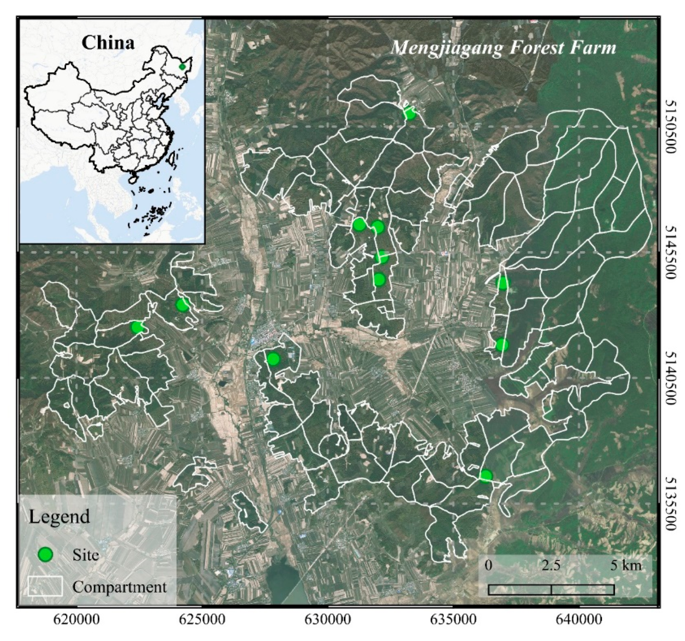
2.1. Study Area

This study was conducted in the Mengjiagang Forest Farm (130°32′42″−130°52′36″ E, 46°20′16″−45°30′50″ N), located in the northeastern area of the Huanan County, Heilongjiang province, China. The forest farm is specifically situated in the western foothills of Wanda mountain. The slope is relatively gentle, most of which is between 10° and 20°. The terrain is higher in the northeast and lower in the southwest, with a maximum, minimum, and average altitude of 575 m, 170 m, and 250 m above sea level, respectively [57]. This area pertains to a temperate continental monsoon climate, and the soil type is mostly dark brown forest soil. The forests are primarily dominated by artificially grown coniferous trees, including Larix olgensis, Pinus sylvestris var. mongolica, and Pinus koraiensis.

2.2. Field Measurement Data

The field survey was carried out in July 2019; a total of 118 square sample plots (30 m × 30 m) with normal growth were established in 11 sites (Figure 1) for long-term growth monitoring (the descriptive statistics of field-measured data are shown in Table 1). The initial planting density of all sites was 3300 stems/ha (spacing 2 m × 1.5 m). The young forest was treated with crown thinning (interval 3−5 years) to adjust the stand’s composition and density. The middle-aged forest and near-mature forest were treated with growth tending (interval 6−10 years) to promote the growth of trees. The intensity of crown thinning is 25−45%, or the accumulation intensity is 15−30%; the intensity of growth tending is 15−30%, or the accumulation intensity is 10−20% [58]. All trees in sample plots with DBH greater than 5 cm were measured by diameter tape. The four-directional canopy width was measured by steel tape, and the values were averaged to obtain the crown width. The total tree height and HCB were measured by Vertex IV Ultrasonic Hypsometer made by Haglöf Sweden. The relative coordinates of the sampled trees were measured according to their relative position to the corner of the plots. In addition, the geographic coordinates of the individual trees and four corners of each plot were thoroughly measured with a real-time kinetic (RTK) global navigation satellite system (GNSS) (UniStrong G10A, China), except for trees having poor GNSS signals which were georeferenced by their relative coordinates.

2.3. Unmanned Aerial Vehicle Laser Scanning Data Acquisition

The RIEGL mini VUX-1UAV LiDAR scanner mounted on the Feima D200 UAV platform was used to obtain UAV-LiDAR data from the 11 sites (from 10–12 July 2019). The working pulse repetition frequency, maximum measuring range, and maximum scanning speed of the scanner were 100 kHz, 250 m, and 100 scans per second, respectively. The scanning angle was controlled within ±60° to reduce the measurement error caused by an immense angle. The flight speed was 5.0 m/s, maneuvering around 80 m of above-ground altitude, and the air route was a cross-transect with overlapping strips of 80 m. The average point cloud density results for each site were between 150 and 270 pt./m2.

2.4. UAV-LiDAR Metrics Extraction

The UAV-LiDAR data processing and metrics extraction can be found in Figure 2. The noise points were masked off manually from the raw LiDAR data, and the remaining points were divided into ground points and non-ground points by using cloth-simulated filtering [59]. To generate digital terrain models (DTMs), the ground points were interpolated by a Kriging spatial interposition method with a 0.5 m pixel size [60]. Then, the normalized height of each point was obtained by subtracting the DTM value from the elevation of all points [61]. We applied a canopy filtering method called graph-based progressive morphological filtering (GPMF), which was used to obtain the canopy height model (CHM) from LiDAR data. GPMF might prevent data pits obtained by traditional methods from damaging the integrity and smoothness of the tree canopy, leading to a large error in the extraction of tree parameters [62]. The resolution of CHM was set to 0.1 m. The individual tree canopies were detected automatically from the CHM using the region-based hierarchical cross-section analysis (RHCSA) algorithm [63]. This algorithm treats CHM as a mountain terrain and uses the crown’s horizontal relation in the vertical direction to detect a single tree.
Tree-to-tree matching generation was performed between field measurements and segmented trees according to spatial position and height difference [2]. If the segmented tree was located within a circular buffer (the corresponding crown radius) around the reference point and the height difference was less than 20% of the plot’s highest height, the segmented tree was designated as the reference tree candidate [64]; then, a unique candidate or nearest individual in multiple candidates was selected as a different candidate to match the reference tree. Eight thousand seven hundred eighty-five (8785) trees in 118 plots were matched correctly with the field data, and the detection rate was 56–100% (mean 76%). After the automatic matching generation, the dead trees and other irrelevant data were removed from the dataset. Finally, the remaining 8364 trees were correctly matched with the field-measured data and utilized for subsequent modeling.
Previous studies have shown that HCB is significantly affected by tree size, competition, and stand characteristics [31,65,66]. In this study, those three categories of predictors were generated from UAV-LiDAR data (Table 2) and used to develop a generalized HCB estimation model (Section 2.5). The indicators of tree size—including LiDAR-derived tree height and crown width—were defined as the maximum height of all LiDAR pulses and calculated by 2 × c r o w n a r e a / π , where c r o w n a r e a was the area of the convex hulls of delineated crowns [15]. Furthermore, distance-independent competition indices were calculated from LiDAR data [67]. The LiDAR-derived relative dimensions of tree height and crown projection area were firstly introduced, including the ratios of a target tree’s height to the maximum and mean tree height ( R H m a x and R H m e a n ) and the ratios of a target tree’s crown area to the maximum, mean, and total crown area ( R C A m a x ,   R C A m e a n and R C A t o t a l ), respectively. Secondly, a measure of competition based on crown areas evaluated at a certain percentage of crown length was expanded and calculated using LiDAR data [68]. The ratio between the subjected and the total crown areas computed at a reference height equal to p % of the height of the subject tree ( h p ) was calculated as a competition index. Finally, the plot-level metrics were generated to characterize the stand conditions, including height percentiles ( H 5 P , H 10 P , …, H 99 P ), variance, standard deviation and coefficient of variation of height ( H v a r P , H s t d P , H c v P ), skewness and kurtosis of height ( H s k w P , H k u r P ), and the proportion of points above the corresponding percentiles ( H 5 P , H 10 P , …, H 99 P ) to the total number of points within a plot ( D 5 P , D 10 P , …, D 99 P ). The candidate variables of this study are given in Table 2.

2.5. Two-Level NLME HCB Model

2.5.1. Base HCB Development

Following previous field-based HCB modeling studies [45], we tested three candidates of HCB models [65,69] for model development (logistic and exponential form). Instead of DBH, we applied C W as the primary predictor ( X = C W ) since DBH mostly cannot be directly extracted from aerial point cloud data due to the canopy obstruction. The following exponential model was originally formulated by Wykoff, et al. (1982) [65] and was found to be the most suitable for our dataset:
        H C B = H [ 1 e x p ( β X ) ]
where H C B and H is height to crown base and total tree height, respectively; X is vectors of stand or tree variables; and β is the estimated parameter vector.
H and C W are closely related to HCB, affecting photosynthesis and interspecific competition of trees, and both can be directly extracted from LiDAR data; hence, they are often used as a predictive variable for the HCB model [4]. As an effort to improve the fitting effect and prediction accuracy of the model, we introduced covariates to reflect the stand quality and competition factors in constructing the based model (Table 2), the predictors could be extended as:
      X = f ( C W , S t a n d . , C o m p . )
where C W , S t a n d . , and C o m p . is the crown width, stand quality factors, and competition factors, respectively.
All covariates were significant and had consistent correlation, which were selected using optimal subset regression. To ensure the simplicity of the model and prevent excessive parameterization and collinearity, one covariate within each variable group was introduced into the model.
The models were fitted to the whole data using nonlinear least-squares regression in R4.0.3 software. Several statistical criteria were used to select the best fitting performance model, including the coefficient of determination (R2), the mean difference (Bias), root mean square error (RMSE), and Akaike information criterion (AIC) as in Dong, et al. (2014) [70].

2.5.2. Two-Level NLME HCB Model

A two-level NLME HCB model was further introduced to consider the random interference of both site- and plot-level variation. The model expression is given below [71]:
H C B j i k = f ( φ i j k , x i j k ) + ε i j k ,   i = 1 , , M ,   j = 1 , , M i ,   k = 1 , , n i j
where the indices i , j , k are the site-level, the plot-level within the site-level, and the observation of an individual tree, respectively; H C B j i k is the height to the crown base of the k t h tree on the j t h plot within the i t h site; M is the number of site; M i is the number of the sample plots within the i t h site; n i j is the number of trees on the j t h plot in the i t h site; f ( . ) is a real-valued and differentiable function of a plot-specific parameter vector φ i j k and a covariate vector x i j k ; and ε i j k represents the within-group error with zero expected value and follows a normal distribution, and has R i j as the positive-definite variance-covariance structure. Furthermore, φ i j k can be expressed as:
φ i j k = A i j k β + B i , j k u i + B i j k u i j ,     u i ~ N ( 0 , ψ 1 ) ,   u i j ~ N ( 0 , ψ 2 )
where β is the p-dimensional fixed-effect parameter vector; u i and u i j are the site- and plot-level random-effects parameter, which assumed to obey the normal distribution with the expectation of zero value and the variance-covariance of ψ 1 and ψ 2 , respectively; and A i j k , B i , j k , and B i j k are respectively the design matrices corresponding to β , u i , and u i j . ε i j k , u i , and u i j are mutually independent.
The most important step for applying a mixed-effects model is to determine which parameters are categorized as fixed effects and random-effects parameters. In this study, all parameter combinations were simulated as mixed parameters with Akaike’s information (AIC), Schawarz’s Bayesian information criterion (BIC), and likelihood (LL) as the main criteria to evaluate the fitting performance.
Further analysis was carried out by selecting a mixed-effect parameter combination having the smallest AIC, BIC, and LL. We performed a likelihood-ratio test (LRT) to avoid overparameterization [72].
The predictions residuals of the NLME HCB model with both site- and plot-level random effects were analyzed for potential spatial autocorrelation and heteroscedasticity. The preliminary analysis showed that heteroscedasticity was detected, but there was no spatial autocorrelation between the observed values. To solve this problem, the following error term variance-covariance matrix structure was analyzed and applied:
R i j = σ 2 G i j 0.5 Γ i j G i j 0.5
where R i j is the variance-covariance matrix of the error term ε i j in the j t h plot within the i t h site ( i = 1 , .   .   . , M ,   j = 1 , , M i ); σ 2 represents the scaling factor of the sample plot error dispersion; G i j 0.5 is a n i j × n i j dimensional diagonal matrix which accounts for the heteroscedasticity of data in the sample plot; Γ i j is a   n i j × n i j dimensional matrix explaining within plot autocorrelation structure of errors. The Γ i j was supposed as an identity matrix since there was not any spatial autocorrelation detected. Therefore, only the effect of heteroscedasticity needed to be considered on the model. Three commonly used variance stability functions were evaluated and compared, including exponential function, power function, and constant plus power function. The results showed that the power variance function with H as the independent variable (Equation (6)) effectively explained the heteroscedasticity in our data.
v a r ( ε i j k ) = σ 2 H i j k 2 γ
where H i j k is the tree height derived from LiDAR data of the k t h tree within the j t h plot and the i t h site; and γ is the estimated parameter.

2.5.3. Prediction and Calibration

Two situations—using fixed-effects only and a mixture of fixed- and random-effects—can be considered when using a two-level NLME model to predict HCB. The fixed-effect only model can also be called a population average or uncalibrated response model. In contrast, the model that contains random effects is typically called a localized or subject-specific model, in which the localizing process is mostly known as model calibration [73]. The uncalibrated model nullifies the random effect parameter and does not need any prior information. The subject-specific models were calibrated by predicting the specific plot and site effects using several sampled trees’ measured attributes from the validation site. The values of random effect parameters were determined by the best linear unbiased prediction (BLUPs) [74]. The expression is as follows:
u ^ i = ψ ^ Z i T ( R ^ i + Z i ψ ^ Z i T ) 1 e i = ψ ^ Z i T ( R ^ i + Z i ψ ^ Z i T ) 1 ( y i y ^ i f i x e d )
where u ^ i = ( u ^ i , u ^ i 1 , u ^ i 2 , , u ^ i M i ) T is a q 1 + M q 2 -dimensional vector of the estimated random-effects parameters for the i t h site; u ^ i is the q 1 -dimensional vector of the estimated value at site level; u ^ i 1 to u ^ i M i are the estimated q 2 -dimensional vectors of the random-effects parameters at the sample plot level; R ^ i is the variance-covariance matrix of within-group errors; Z i is the design matrix of the partial derivatives of the nonlinear function corresponding to the random parameters; and ψ ^ is an ( q 1 + M q 2 ) × ( q 1 + M q 2 ) block diagonal matrix consisting of ψ ^ 1 and ψ ^ 2 , the two estimated variance-covariance matrices for the random effects parameters u i and u i j ; and e i is the error terms of the predicted by the fixed effects parameters of the mixed-effects models. The maximum likelihood method of NLME function in NLME package [75] in the software R4.0.3 was employed to estimate the model parameters.

2.6. Model Assessment

The prediction applicability of the HCB models including the base model, uncalibrated model, and calibrated NLME model were evaluated by using independent observation data. In this study, all data was utilized for model development, and the leave-one-site-out cross-validation (LOOCV) was used to test the independence and adaptability of the model. Base model, uncalibrated model, and calibrated NLME model were compared using the average statistics of cross-validation within a sample plot. The performance of the model was evaluated by calculating four model validation statistics (Bias, Bias%, MAE, and MAE%) as follows:
B i a s =   ( H C B t H C B ^ t ) n
B i a s % = B i a s m e a n ( H C B ) × 100
M A E =   | H C B t H C B ^ t | n
M A E % = M A E m e a n ( H C B ) × 100
where H C B t and H C B ^ t is the t t h observed and predicted height to crown base ( t = 1 , ,   N ); N is number of the observations; and m e a n ( H C B ) is the mean value of HCB observations.

2.7. Comparison of Different Sampling Strategies

The mixed-effect model’s calibration was calculated using the field-measured HCB of some multiple sample trees as the prior information to predict the specific random-effects parameters. Therefore, we proposed multilevel prediction (both site- and plot-level), which is convenient for application across different scales yet still provides a high accuracy [76].

2.7.1. Site-Level Calibration

The site-level calibration was achieved by setting the plot-level random parameter to zero, which can be completed without utilizing sample plots. Hence it is more suitable for large-scale and efficient prediction. Generally, the larger the calibration sample size, the more accurate the calibration result. However, sampling a large number of sample trees only to calculate the random-effect parameters is impractical. Hence, we proposed a simpler sampling strategy:
Selecting 1−50 trees randomly per site.
The simulation was repeated 1000 times to calculate the average results, preventing the prediction from being biased.

2.7.2. Plot-Level Calibration

Compared with the site-level calibration, plot-level calibration has higher prediction accuracy since it considers the random effects of both site-level and plot-level nested within the site. Hence, it is more suitable for small-scale and high-precision prediction. Considering the measurement cost and potential error of UAV-LiDAR in extracting forest structure parameters, eight sampling strategies with different subsampling schemes were proposed as follows:
Type I: Selecting l trees randomly per plot ( l : 2, 3, …, 18).
Type II: Selecting l largest trees per plot ( l : 2, 3, …, 18).
Type III: Selecting l smallest trees per plot ( l : 2, 3, …, 18).
Type IV: Selecting l medium-size trees (defined as the sample tree whose DBH is closest to the quadratic mean diameter of stand) per plot ( l : 2, 3, …, 18).
Type V: Selecting l 2 largest trees and l 2 smallest trees per plot ( l : 2, 4, …, 18).
Type VI: Selecting l 2 largest trees and l 2 medium-size trees per plot ( l : 2, 4, …, 18).
Type VII: Selecting l 2 smallest trees and l 2 medium-size trees per plot ( l : 2, 4, …, 18).
Type VIII: Selecting l 3 largest trees, l 3 smallest trees and l 3 medium-size trees per plot ( l : 3, 6, …, 18).
Bias% and MAE% were used to assess the prediction accuracy under different sampling strategies and sizes. The source code for assessment and an example for plot-level sampling in R 4.0.3 are shown in Supplementary.

3. Results

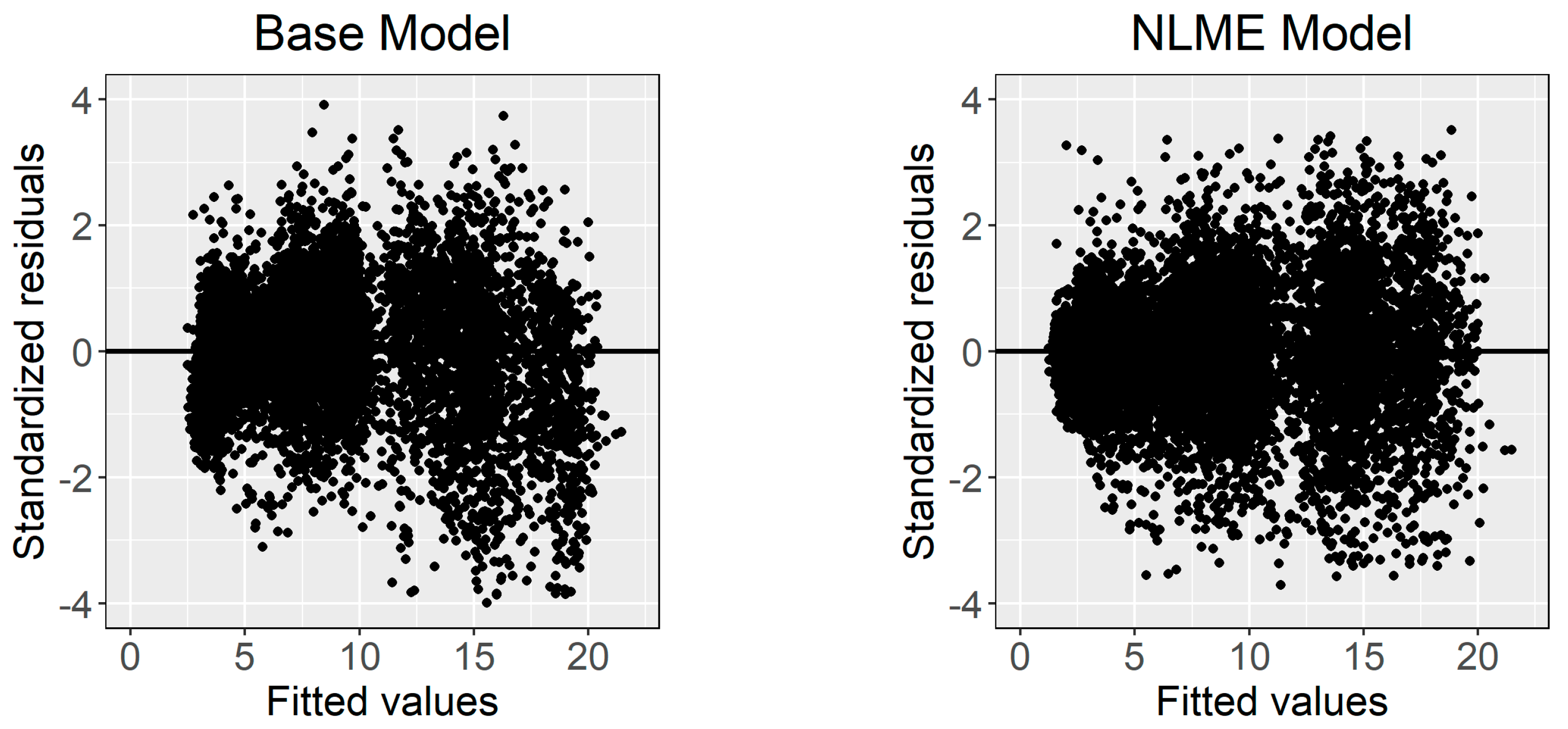
3.1. Base Model Development

The optimal subset method was utilized to select covariates and H , C W , C C p 75 , and H 99 P were used as predictive variables to expand the basic model since they have the largest value of R2 and the smallest value of RMSE, Bias, and AIC. The C C p 75 —the ratio of the target tree’s crown area to the sum of all crown areas above their 75% relative tree’s total height within the sample plot—can commendably reflect the competitive situation [77]. Meanwhile, the elevation of the 99%-point cloud of the subject plot ( H 99 P ) was used to describe the stand variation’s effect on HCB. The final multivariate model is as follows:
H C B i j k = H i j k × ( 1 exp ( β 0 + β 1 × C W i j k + β 2 × C C p 75 + β 3 × H 99 P ) ) + ε i j k
where H C B i j k , H i j k , and C W i j k are height to crown base, total tree height, and crown width of the k t h tree in the j t h plot within the i t h site, respectively; β 0 , β 1 , β 2 , and β 3 are model parameters to be determined; and ε i j k is an error term. The parameter estimates of the base model were presented in Section 3.3.
All model parameters are significant, and the model fitting has substantially improved after adding covariates (Table 3). The basic model explained more variations of HCB after extending the site quality and competition indices, which could be useful for the further construction of the two-level mixed effect model.

3.2. Two-Level Nonlinear Mixed-Effects HCB Model

The influences of site and plot variation on HCB were considered in model (12). There were four parameters ( β 0 β 3 ) considered in the base model, yielding 15 different combinations of random-effects parameters. However, only nine combinations of parameter estimates were successfully converged. The model had the smallest AIC value (25,565) and the highest fitting accuracy (R2 = 0.9424 and RMSE = 1.1282) when β 0 and β 1 were included as the random effect parameters. All parameter estimates can be found in Section 3.3. The specific form is as follows:
H C B i j k = H i j k × ( 1 exp ( β 0 + u 0 i + u 0 i j + ( β 1 + u 1 i + u 1 i j ) × C W i j k + β 2 × C C p 75 + β 3 × H 99 P ) ) + ε i j k
where:
u i = [ u 0 i u 1 i ] ~ N { [ 0 0 ] ,   ψ ^ 1 }
u i j = [ u 0 i j u 1 i j ] ~ N { [ 0 0 ] ,   ψ ^ 2 }
ε i j k ~ N ( 0 , R i j = G i j 0.5 Γ i j G i j 0.5 )
G i j = d i a g ( σ 2 H i j 1 2 γ   , , σ 2 H i j k 2 γ   )
Γ i j = I i j
where u 0 i and u 1 i are the random effects caused by the i t h site on β 0 and β 1 , respectively; u 0 i j and u 1 i j are the random effects caused by the   j t h sample plot nested in the i t h site on β 0 and β 1 , respectively; and other symbols have been described in previous sections. Figure 3 shows the standardized residuals distribution of the base model and calibrated NLME model. The weighted power function significantly stabilized the heteroscedasticity. The values of the power variance functions are listed in Table 3.

3.3. Parameter Estimates

All parameters estimated in the NLME HCB model were statistically significant (p < 0.05). The specific parameter estimation values and fitting statistics of each model are shown in Table 3. The likelihood ratio test (LRT) of the base nonlinear model (12) and the NLME model (13) showed that the mixed effect model was statistically significant (p < 0.0001), indicating that the plot variation had a significant random effect on HCB.

3.4. Model Assessment

The prediction ability of the base model, NLME model with fixed parameters only (uncalibrated model), and NLME model with fixed and random parameters (calibrated model) was assessed by the leave-one-site-out cross-validation method, and the results were compared and are demonstrated in Table 4. The calibrated NLME model had the best adaptability and stability performance compared to the two others, with the MAE and MAE% as low as 0.89% and 9.71%, respectively. The base model’s performance was worse than the NLME model but slightly better than the uncalibrated model. Figure 4 visualized that the prediction calculated by the calibrated NLME model is more consistent along the trend line Y = X than the base and uncalibrated model. In addition, the base and uncalibrated models show an apparent overestimation in predicting the individual trees with lower HCB, which has been effectively solved by the calibrated NLME model (Figure 4).
Moreover, the prediction accuracy of the three models was scrutinized across 15 diameter classes (Figure 5). The upper limit exclusion method was used for diameter class integration with 2 cm equal difference (i.e., [5,7), [7,9), ...). The trees with DBH more than 33 cm are classified into 34 diameter classes. The uncalibrated model shows the worst accuracy among all methods with the MAE value ranging from 0.69 to 1.88. Meanwhile, the calibrated NLME model has the highest prediction accuracy with MAE ranging from 0.61 to 1.47, having approximately a 0.09 to 0.51 decrease compared with the uncalibrated model. The MAE% values were the worst for the low diameter classes and were found to be decreased with the increasing DBH. The calibrated NLME model presented the best prediction accuracies across different diameter classes. It is worth mentioning that the base model is generally underestimated in the lower and larger diameter classes but overestimated in the medium diameter classes (Figure 5). Underestimation and overestimation lead to the “canceling out” of positive and negative deviation, which also explains why the base model has a lower bias (Table 4). Figure 5 also shows that the error range and prediction accuracy of the calibrated NLME model are relatively stable, while the performance of the uncalibrated model is often worse than that of the base model. The calibrated NLME model provides a clear visualization of the whole population’s average responses and the changes between different levels. The estimation was consistent across different diameter classes, proving the mixed effect model’s robustness in predicting the property’s change of variables.

3.5. Comparison of Different Sampling Strategies

3.5.1. Site-Level Calibration

We randomly selected 1−50 trees from each site for site-level local calibration using the BLUPs theory, which is repeated continuously for 1000 times to calculate the average of the error statistics (MAE% and Bias%). The results of the calibration response mode are shown in Figure 6. For site-level calibration, only when the subsample is more than five, the prediction effect is better than that of the uncalibrated model. MAE% gradually decreased with the increase of sampling number. The overall trend of Bias% is similar to MAE%, although there are slight fluctuations. When the subsample size is 15, MAE% was reduced to 11.5%. Increasing the number of samples was not significant to improve the model’s accuracy but it will increase the cost of measurement. Therefore, there is always be a tradeoff between the cost and accuracy, in which selecting 15 trees randomly for site-level calibration might be recommended as the best compromise between the two.

3.5.2. Plot-Level Calibration

Eight BLUPs strategies in local plot-level calibration were proposed to improve the model’s accuracy. The calibration prediction results were visualized by two error statistics (Bias% and MAE%) and shown in Figure 7. Apart from type III, all sampling strategies had similar trends, in which the calibration performance improves with the increase of sample size, and the subject-specific predictions obtained higher accuracy than uncalibrated predictions, even though only a small number of trees (i.e., two) are used as the basis for the random effect predictions. The type VI sampling strategy obtained the smallest MAE% when the prediction pre-measured sub-sample size was less than eight trees, while similar prediction performance was delivered by both type VI and type IV when the sub-sample size was more than eight trees. The largest MAE% was always acquired by the type III sampling strategy. For the type VI, more stable prediction was obtained after including seven sampling trees, even the results were still outperformed by other sampling strategies. In addition, a paired t-test was used to compare the calibrated NLME predictions using between 6 trees and 18 trees for calculating the random parameters, and the result was found to be not statistically significant. Hence, using six sampling trees in the HCB model calibration might present the most optimum results when the time and cost efficiency is considered. A relatively high prediction accuracy with a low measurement cost might be achieved by sampling the three largest trees and three medium-size trees (type VI) from each sample plot.

4. Discussion

As an essential individual tree variable, height to crown base (HCB) can effectively reflect the crown size, subsequently affecting the forest’s vitality, wood quality, and commercial value of trees [30]. Hence, it is very important to obtain accurate and efficient data of HCB, which has been conveniently facilitated by utilizing remote sensing data. However, due to the tree canopy occlusion and point cloud density limitation, acquiring a stable method to accurately and directly extract the HCB from LiDAR data remains challenging. Therefore, this study was intended to develop and provide an accurate HCB model using a generalized NLME method.
In this study, three commonly used HCB models were evaluated to construct the HCB model based on LiDAR data [65,69]. Tree height ( H ) and crown width ( C W ) were used as the primary predictors since they account for the most variations on HCB and are relatively easy to be accurately extracted [46]. Furthermore, stand quality and interspecific competition were added to the model as potential predictors. In previous forest modeling studies, dominant height ( H d ) was the most commonly used variable to represent stand quality [78,79]. However, the LiDAR-based relative percentile height can be directly extracted from each sample plot to replace H d and was not affected by the calculation method; hence, it is more suitable for our model. All combinations of stand and competition metrics were analyzed and used to finally determine both H 99 P and C C p 75 , which are novel to LiDAR-derived variables. The RMSE decreased by 38.46% after these two covariates were introduced into the model, showing that the covariates extension was effective and could be further used for the random effects. The negative parameters of both stand and competition index indicated that the HCB was positively correlated with the stand quality and competition size. This is ecologically reasonable since the better the stand conditions, the higher the tree height, consequently promoting the crown’s overall upward movement and increasing the HCB. The competition index expressed by C C p 75 was constantly recognized in the description of the crown competition. The larger the C C p 75 of the targeted trees, the weaker the competition ability, and the more difficult for the trees to acquire sunlight, water, and soil nutrients, resulting in a shorter and smaller crown [80,81]. The proposed multivariable generalized base model has high adaptability and was found to be effective for detecting the variation of HCB with the same height and crown width. The selected experimental sites have similar geographical conditions; hence, we did not consider the influence of altitude, terrain, and slope on the developed model.
The nonlinear mixed effect (NLME) model can reflect the potential variations among different levels and has been widely utilized to construct the HCB model [45,47,66]. In this study, the data was sampled from an extensive and widely distributed area. Hence, applying a two-level nested random effect model will be appropriate to describe the specific effect of the plot and site variations on HCB. Generally, the mixed effect model’s convergence becomes harder to be achieved as the number of random effect parameters increases, especially when the model contains more than two parameters [82]. In this study, all possible combinations of random effect parameters were considered. The HCB model obtained the smallest AIC and the highest R2 after the random effects were added into the intercept β 0 and the regression coefficient β 1 of the crown width. The calibrated model’s accuracy was significantly higher than that of the generalized base model, which was indicated by LRT. In addition, three functions were compared for selecting the appropriate weighting function, in which the power function was finally chosen due to its simplicity and convenient application.
The leave-one-site-out cross-validation method was applied to assess the independence and applicability of the models. As shown in Table 4, the introduction of random effects has greatly improved the model’s prediction accuracy, even after it was scrutinized throughout various diameter classes (Figure 5). The relative bias of the calibrated NLME model was closer to zero and relatively more stable than the other two models. However, the model generally produced a larger MAE% and Bias% in small diameter classes (i.e., 6−8 diameter classes). The possible reason is that the younger trees often have no crown overlap between individuals, leading to less competition among trees. Thus, the lower canopy’s living branches have more opportunities to absorb sunlight for photosynthesis, which contributes to enhancing their growth activity. Furthermore, HCB is usually more affected by non-natural factors (e.g., tending and pruning activity) [33]; hence, various management measures should be considered to accurately predict the HCB of young trees.
Compared with the recently developed HCB models which are only based on field-measured attributes [45,81], our LiDAR-based models might provide a more highly efficient prediction that requires less effort to obtain the input information. Several researches [41,42,83] extracted HCB directly from LiDAR data. However, the algorithms are not applicable for large-scale estimation. In addition, some studies [46,52] include field-measured variables (i.e., DBH) in building LiDAR-based HCB models that was unnecessary in our study, which improves the flexibility of the model.
We proposed both site- and plot-level model calibration to improve the flexibility of model application throughout different scale and accuracy requirements. Site-level calibration does not need additional plot information; hence, it is convenient for efficient prediction in large areas. Therefore, we proposed a simple sampling strategy (1−50 trees randomly selected per site). The model’s prediction accuracy will improve as the number of sampled trees per plot increases [83]. The results showed that randomly selecting 15 trees from each site may be a good option when both precision and cost are considered. In addition, for plot-level calibration, eight complex sampling strategies and various numbers of subsampled trees were assessed by leave-one-site-out cross-validation, aiming to ascertain the best calibration scheme for predicting the HCB of new stands. The results showed that using the smallest trees for model calibration (type III) obtained the worst result, consistent with other studies [45,46,51]. This may be attributed to the fact that some fixed-effect variables in the NLME HCB model have reflected the variation of small-size trees; hence, the type III sampling strategy did not provide any additional information for calibration. On the contrary, using the largest trees and medium-size trees (type VI sampling strategy) obtained the best calibration results. It is worth recalling that type IV was worse than type VI when the sample size was small, but the difference between them gradually decreased as the sampling size increased. However, this correction strategy is necessary to obtain the DBH of each tree in the sample plot, which undoubtedly increases the workload of the field measurement. The result of random sampling (type I) is also given, which is only slightly worse than type VI (Figure 7). It can be used when the field-measured DBH is not available. Generally, four to nine sample trees are used for mixed effect model plot-level calibration to ensure a tradeoff between the model predictability and inventory cost [79,84]. This study suggests that using six trees for NLME model calibration is appropriate when prediction accuracy and measurement cost are considered. Adding more sample trees in model calibration seems inefficient since it brings an insignificant improvement to the model performance and yet causes a remarkable increase in inventory cost.
This study only used the correctly matched individual trees for constructing and evaluating the model. However, the commission and omission errors cannot be ignored since they might affect the method’s actual application. The segmentation errors often increase with stand density, which mainly miss detection of suppressed trees, especially in young forests [85]. Therefore, a careful application should be conducted when applying this method in high-density young forests. In the future, a segmentation algorithm suitable for the high-density forest will substantially improve the application of this model.

5. Conclusions

Larix olgensis is one of the main afforestation tree species in Northeast China, which has fast growth and provides high timber output. In this paper, a generalized nonlinear mixed effect HCB model of larch plantation was established using UAV-LiDAR data. The newly developed model could complement the missing HCB data in forest inventory and reduce the field workload without ignoring the prediction accuracy. The tree- and plot-level LiDAR-derived metrics (i.e., H , C W , C C p 75 and H 99 P ) were introduced into the base model, which significantly improved the model’s ability to explain the HCB variation. The introduction of two-level random effects greatly improved the application ability and prediction accuracy of the model. The newly developed model not only has an important significance for HCB prediction, but also supplies a more flexible and convenient method for forest application based on UAVs.

Supplementary Materials

The following are available online at https://0-www-mdpi-com.brum.beds.ac.uk/article/10.3390/rs13091834/s1. R code for assessment and an example for plot-level sampling are shown in Supplementary.

Author Contributions

Conceptualization, X.L., Y.H., L.D. and F.L.; methodology, X.L., Y.H. and L.D.; software, X.L., L.X. and Y.H.; validation, F.R.A.W., Y.H. and L.X.; formal analysis, X.L. and Y.H.; investigation, X.L., Y.H., F.R.A.W. and L.X.; resources, L.D. and F.L.; data curation, L.D. and F.L.; writing—original draft preparation, X.L.; writing—review and editing, X.L., F.R.A.W., Y.H., L.X., L.D. and F.L.; visualization, X.L. and Y.H.; supervision, L.D. and F.L.; project administration, L.D. and F.L.; funding acquisition, F.L. All authors have read and agreed to the published version of the manuscript.

Funding

This research was supported by the National Key R&D Program of China (grant number 2017YFD0600402); Provincial Funding for the National Key R&D Program of China in Heilongjiang Province (grant number GX18B041); Fundamental Research Funds for the Central Universities (grant number 2572020DR03); and the Heilongjiang Touyan Innovation Team Program (Technology Development Team for High-efficient Silviculture of Forest Resources).

Data Availability Statement

Not Applicable.

Acknowledgments

The authors would like to thank the faculty and students of the Department of Forest Management, Northeast Forestry University (NEFU), China, who collected and provided the data for this study.

Conflicts of Interest

The authors declare no conflict of interest.

References

  1. Fang, J.; Chen, A.; Peng, C.; Zhao, S.; Ci, L. Changes in Forest Biomass Carbon Storage in China between 1949 and 1998. Science 2001, 292, 2320–2322. [Google Scholar] [CrossRef] [PubMed]
  2. Zhao, K.; Suarez, J.C.; Garcia, M.; Hu, T.; Wang, C.; Londo, A. Utility of multitemporal lidar for forest and carbon monitoring: Tree growth, biomass dynamics, and carbon flux. Remote Sens. Environ. 2018, 204, 883–897. [Google Scholar] [CrossRef]
  3. Liang, X.; Hyyppä, J.; Kaartinen, H.; Lehtomäki, M.; Pyörälä, J.; Pfeifer, N.; Holopainen, M.; Brolly, G.; Francesco, P.; Hackenberg, J.; et al. International benchmarking of terrestrial laser scanning approaches for forest inventories. ISPRS J. Photogramm. Remote Sens. 2018, 144, 137–179. [Google Scholar] [CrossRef]
  4. West, B.W. Tree and Forest Measurement; Springer: Berlin/Heidelberg, Germany, 2009. [Google Scholar]
  5. Tomppo, E.; Olsson, H.; Ståhl, G.; Nilsson, M.; Hagner, O.; Katila, M. Combining national forest inventory field plots and remote sensing data for forest databases. Remote Sens. Environ. 2008, 112, 1982–1999. [Google Scholar] [CrossRef]
  6. Goetz, S.J.; Hansen, M.; Houghton, R.A.; Walker, W.; Laporte, N.; Busch, J. Measurement and monitoring needs, capabilities and potential for addressing reduced emissions from deforestation and forest degradation under REDD+. Environ. Res. Lett. 2015, 10, 123001. [Google Scholar] [CrossRef]
  7. Labrecque, S.; Fournier, R.A.; Luther, J.E.; Piercey, D. A comparison of four methods to map biomass from Landsat-TM and inventory data in western Newfoundland. For. Ecol. Manag. 2006, 226, 129–144. [Google Scholar] [CrossRef]
  8. Chen, B.; Cao, J.; Wang, J.; Wu, Z.; Tao, Z.; Chen, J.; Yang, C.; Xie, G. Estimation of rubber stand age in typhoon and chilling injury afflicted area with Landsat TM data: A case study in Hainan Island, China. For. Ecol. Manag. 2012, 274, 222–230. [Google Scholar] [CrossRef]
  9. Lu, D. The potential and challenge of remote sensing-based biomass estimation. Int. J. Remote Sens. 2006, 27, 1297–1328. [Google Scholar] [CrossRef]
  10. Lim, K.; Treitz, P.; Wulder, M.; St-Onge, B.T.; Flood, M. LiDAR remote sensing of forest structure. Prog. Phys. Geogr. 2003, 27, 88–106. [Google Scholar] [CrossRef] [Green Version]
  11. Nelson, R. How did we get here? An early history of forestry lidar. Can. J. Remote Sens. 2013, 39, 6–17. [Google Scholar] [CrossRef] [Green Version]
  12. Mutlu, M.; Popescu, S.C.; Zhao, K. Sensitivity analysis of fire behavior modeling with LIDAR-derived surface fuel maps. For. Ecol. Manag. 2008, 256, 289–294. [Google Scholar] [CrossRef]
  13. García, M.; Gajardo, J.; Riaño, D.; Zhao, K.; Martín, P.; Ustin, S. Canopy clumping appraisal using terrestrial and airborne laser scanning. Remote Sens. Environ. 2015, 161, 78–88. [Google Scholar] [CrossRef]
  14. Véga, C.; Renaud, J.-P.; Durrieu, S.; Bouvier, M. On the interest of penetration depth, canopy area and volume metrics to improve Lidar-based models of forest parameters. Remote Sens. Environ. 2016, 175, 32–42. [Google Scholar] [CrossRef]
  15. Coomes, D.A.; Dalponte, M.; Jucker, T.; Asner, G.P.; Banin, L.F.; Burslem, D.F.R.P.; Lewis, S.L.; Nilus, R.; Phillips, O.L.; Phua, M.-H.; et al. Area-based vs. tree-centric approaches to mapping forest carbon in Southeast Asian forests from airborne laser scanning data. Remote Sens. Environ. 2017, 194, 77–88. [Google Scholar] [CrossRef] [Green Version]
  16. Lin, Y.; Hyyppa, J.; Jaakkola, A. Mini-UAV-Borne LIDAR for Fine-Scale Mapping. IEEE Geosci. Remote Sens. Lett. 2011, 8, 426–430. [Google Scholar] [CrossRef]
  17. Wallace, L.; Lucieer, A.; Watson, C.; Turner, D. Development of a UAV−LiDAR System with Application to Forest Inventory. Remote Sens. 2012, 4, 1519–1543. [Google Scholar] [CrossRef] [Green Version]
  18. Jaakkola, A.; Hyyppä, J.; Yu, X.; Kukko, A.; Kaartinen, H.; Liang, X.; Hyyppä, H.; Wang, Y. Autonomous Collection of Forest Field Reference—The Outlook and a First Step with UAV Laser Scanning. Remote Sens. 2017, 9, 785. [Google Scholar] [CrossRef] [Green Version]
  19. Guo, Q.; Su, Y.; Hu, T.; Zhao, X.; Wu, F.; Li, Y.; Liu, J.; Chen, L.; Xu, G.; Lin, G.; et al. An integrated UAV-borne lidar system for 3D habitat mapping in three forest ecosystems across China. Int. J. Remote Sens. 2017, 38, 2954–2972. [Google Scholar] [CrossRef]
  20. Bhardwaj, A.; Sam, L.; Akanksha; Martín-Torres, F.J.; Kumar, R. UAVs as remote sensing platform in glaciology: Present applications and future prospects. Remote Sens. Environ. 2016, 175, 196–204. [Google Scholar] [CrossRef]
  21. Kotivuori, E.; Kukkonen, M.; Mehtätalo, L.; Maltamo, M.; Korhonen, L.; Packalen, P. Forest inventories for small areas using drone imagery without in-situ field measurements. Remote Sens. Environ. 2020, 237, 111404. [Google Scholar] [CrossRef]
  22. Jaakkola, A.; Hyyppä, J.; Kukko, A.; Yu, X.; Kaartinen, H.; Lehtomäki, M.; Lin, Y. A low-cost multi-sensoral mobile mapping system and its feasibility for tree measurements. ISPRS J. Photogramm. Remote Sens. 2010, 65, 514–522. [Google Scholar] [CrossRef]
  23. Lu, X.; Guo, Q.; Li, W.; Flanagan, J. A bottom-up approach to segment individual deciduous trees using leaf-off lidar point cloud data. ISPRS J. Photogramm. Remote Sens. 2014, 94, 1–12. [Google Scholar] [CrossRef]
  24. Dalponte, M.; Ørka, H.O.; Ene, L.T.; Gobakken, T.; Næsset, E. Tree crown delineation and tree species classification in boreal forests using hyperspectral and ALS data. Remote Sens. Environ. 2014, 140, 306–317. [Google Scholar] [CrossRef]
  25. Torresan, C.; Berton, A.; Carotenuto, F.; Di Gennaro, S.F.; Gioli, B.; Matese, A.; Miglietta, F.; Vagnoli, C.; Zaldei, A.; Wallace, L. Forestry applications of UAVs in Europe: A review. Int. J. Remote Sens. 2017, 38, 2427–2447. [Google Scholar] [CrossRef]
  26. Liang, X.; Kankare, V.; Hyyppä, J.; Wang, Y.; Kukko, A.; Haggrén, H.; Yu, X.; Kaartinen, H.; Jaakkola, A.; Guan, F.; et al. Terrestrial laser scanning in forest inventories. ISPRS J. Photogramm. Remote Sens. 2016, 115, 63–77. [Google Scholar] [CrossRef]
  27. Gholz, H.L.; Ewel, K.C.; Teskey, R.O. Water and forest productivity. For. Ecol. Manag. 1990, 30, 1–18. [Google Scholar] [CrossRef]
  28. Hasenauer, H.; Monserud, R.A. A crown ratio model for Austrian forests. For. Ecol. Manag. 1996, 84, 49–60. [Google Scholar] [CrossRef]
  29. Antos, J.A.; Parish, R.; Nigh, G.D. Effects of neighbours on crown length of Abies lasiocarpa and Picea engelmannii in two old-growth stands in British Columbia. Can. J. For. Res. 2010, 40, 638–647. [Google Scholar] [CrossRef]
  30. Sharma, R.P.; Bílek, L.; Vacek, Z.; Vacek, S. Modelling crown width–diameter relationship for Scots pine in the central Europe. Trees 2017, 31, 1875–1889. [Google Scholar] [CrossRef]
  31. Monserud, R.A.; Sterba, H. A basal area increment model for individual trees growing in even- and uneven-aged forest stands in Austria. For. Ecol. Manag. 1996, 80, 57–80. [Google Scholar] [CrossRef]
  32. Kuprevicius, A.; Auty, D.; Achim, A.; Caspersen, J.P. Quantifying the influence of live crown ratio on the mechanical properties of clear wood. Forestry 2013, 86, 361–369. [Google Scholar] [CrossRef] [Green Version]
  33. Yan, Y.; Wang, J.; Jiang, L. Construction of the height to crown base mixed model for Korean pine. J. Beijing For. Univ. 2020, 42, 28–36. [Google Scholar]
  34. Sharma, R.P.; Vacek, Z.; Vacek, S. Individual tree crown width models for Norway spruce and European beech in Czech Republic. For. Ecol. Manag. 2016, 366, 208–220. [Google Scholar] [CrossRef]
  35. Fu, L.; Sharma, R.P.; Hao, K.; Tang, S. A generalized interregional nonlinear mixed-effects crown width model for Prince Rupprecht larch in northern China. For. Ecol. Manag. 2017, 389, 364–373. [Google Scholar] [CrossRef]
  36. Crecente-Campo, F.; Álvarez-González, J.G.; Castedo-Dorado, F.; Gómez-García, E.; Diéguez-Aranda, U. Development of crown profile models for Pinus pinaster Ait. and Pinus sylvestris L. in northwestern Spain. Forestry 2013, 86, 481–491. [Google Scholar] [CrossRef] [Green Version]
  37. Ritson, P.; Sochacki, S. Measurement and prediction of biomass and carbon content of Pinus pinaster trees in farm forestry plantations, south-western Australia. For. Ecol. Manag. 2003, 175, 103–117. [Google Scholar] [CrossRef]
  38. Andersen, H.-E.; McGaughey, R.J.; Reutebuch, S.E. Estimating forest canopy fuel parameters using LIDAR data. Remote Sens. Environ. 2005, 94, 441–449. [Google Scholar] [CrossRef]
  39. Temesgen, H.; Lemay, V.; Mitchell, S.J. Tree crown ratio models for multi-species and multi-layered stands of southeastern British Columbia. For. Chron. 2005, 81, 133–141. [Google Scholar] [CrossRef]
  40. Mcroberts, R.E.; Hahn, J.T.; Hefty, G.J.; Cleve, J.R.V. Variation in forest inventory field measurements. Can. J. For. Res. 1994, 24, 1766–1770. [Google Scholar] [CrossRef]
  41. Maltamo, M.; Bollandsås, O.M.; Vauhkonen, J.; Breidenbach, J.; Gobakken, T.; Næsset, E. Comparing different methods for prediction of mean crown height in Norway spruce stands using airborne laser scanner data. Forestry 2010, 83, 257–268. [Google Scholar] [CrossRef]
  42. Vauhkonen, J. Estimating crown base height for Scots pine by means of the 3D geometry of airborne laser scanning data. Int. J. Remote Sens. 2010, 31, 1213–1226. [Google Scholar] [CrossRef]
  43. Luo, L.; Zhai, Q.; Su, Y.; Ma, Q.; Kelly, M.; Guo, Q. Simple method for direct crown base height estimation of individual conifer trees using airborne LiDAR data. Opt. Express 2018, 26, 562–578. [Google Scholar] [CrossRef]
  44. Solberg, S.; Naesset, E.; Bollandsas, O.M. Single Tree Segmentation Using Airborne Laser Scanner Data in a Structurally Heterogeneous Spruce Forest. Photogramm. Eng. Remote Sens. 2006, 72, 1369–1378. [Google Scholar] [CrossRef]
  45. Fu, L.; Zhang, H.; Sharma, R.P.; Pang, L.; Wang, G. A generalized nonlinear mixed-effects height to crown base model for Mongolian oak in northeast China. For. Ecol. Manag. 2017, 384, 34–43. [Google Scholar] [CrossRef]
  46. Yang, Z.; Liu, Q.; Luo, P.; Ye, Q.; Sharma, R.P.; Duan, G.; Zhang, H.; Fu, L. Nonlinear mixed-effects height to crown base model based on both airborne LiDAR and field datasets for Picea crassifolia Kom trees in northwest China. For. Ecol. Manag. 2020, 474, 118323. [Google Scholar] [CrossRef]
  47. Grégoire, T.G.; Schabenberger, O.; Barrett, J.P. Linear modelling of irregularly spaced, unbalanced, longitudinal data from permanent-plot measurements. Can. J. For. Res. 1995, 25, 137–156. [Google Scholar] [CrossRef]
  48. Næsset, E.; Økland, T. Estimating tree height and tree crown properties using airborne scanning laser in a boreal nature reserve. Remote Sens. Environ. 2002, 79, 105–115. [Google Scholar] [CrossRef]
  49. Lindstrom, M.; Bates, D. Nonlinear mixed effects models for repeated measures data. Biometrics 1990, 46, 673–687. [Google Scholar] [CrossRef] [PubMed]
  50. Hall, D.B.; Clutter, M. Multivariate multilevel nonlinear mixed effects models for timber yield predictions. Biometrics 2004, 60, 16–24. [Google Scholar] [CrossRef] [PubMed]
  51. Fu, L.; Duan, G.; Ye, Q.; Meng, X.; Luo, P.; Sharma, R.P.; Sun, H.; Wang, G.; Liu, Q. Prediction of Individual Tree Diameter Using a Nonlinear Mixed-Effects Modeling Approach and Airborne LiDAR Data. Remote Sens. 2020, 12, 1066. [Google Scholar] [CrossRef] [Green Version]
  52. Maltamo, M.; Karjalainen, T.; Repola, J.; Vauhkonen, J. Incorporating tree-and stand-level information on crown base height into multivariate forest management inventories based on airborne laser scanning. Silva Fenn. 2018, 52, 10006. [Google Scholar] [CrossRef]
  53. Zhang, H.; Zhou, X.; Gu, W.; Wang, L.; Li, W.; Gao, Y.; Wu, L.; Guo, X.; Tigabu, M.; Xia, D.; et al. Genetic stability of Larix olgensis provenances planted in different sites in northeast China. For. Ecol. Manag. 2021, 485, 118988. [Google Scholar] [CrossRef]
  54. Peng, W.; Pukkala, T.; Jin, X.; Li, F. Optimal management of larch (Larix olgensis A. Henry) plantations in Northeast China when timber production and carbon stock are considered. Ann. For. Sci. 2018, 75, 63. [Google Scholar] [CrossRef] [Green Version]
  55. Zhou, Z.; Wang, C.; Ren, C.; Sun, Z. Effects of thinning on soil saprotrophic and ectomycorrhizal fungi in a Korean larch plantation. For. Ecol. Manag. 2020, 461, 117920. [Google Scholar] [CrossRef]
  56. State Forestry and Grassland Administration. The Ninth Forest Resource Survey Report (2014–2018); China Forestry Press: Beijing, China, 2019. [Google Scholar]
  57. Gao, H.; Bi, H.; Li, F. Modelling conifer crown profiles as nonlinear conditional quantiles: An example with planted Korean pine in northeast China. For. Ecol. Manag. 2017, 398, 101–115. [Google Scholar] [CrossRef]
  58. Heilongjiang Provincial Bureau of standards and Metrology. Local Standard of Heilongjiang Province—Technical Regulation for Forest Cutting and Regeneration; Heilongjiang Provincial Bureau of standards and Metrology: Qiqihar, China, 1988. [Google Scholar]
  59. Zhang, W.; Qi, J.; Wan, P.; Wang, H.; Xie, D.; Wang, X.; Yan, G. An Easy-to-Use Airborne LiDAR Data Filtering Method Based on Cloth Simulation. Remote Sens. 2016, 8, 501. [Google Scholar] [CrossRef]
  60. Guo, Q.; Li, W.; Yu, H.; Alvarez, O. Effects of Topographic Variability and Lidar Sampling Density on Several DEM Interpolation Methods. Photogramm. Eng. Remote Sens. 2010, 76, 701–712. [Google Scholar] [CrossRef] [Green Version]
  61. Li, W.; Guo, Q.; Jakubowski, M.K.; Kelly, M. A New Method for Segmenting Individual Trees from the Lidar Point Cloud. Photogramm. Eng. Remote Sens. 2012, 78, 75–84. [Google Scholar] [CrossRef] [Green Version]
  62. Hao, Y.; Zhen, Z.; Li, F.; Zhao, Y. A graph-based progressive morphological filtering (GPMF) method for generating canopy height models using ALS data. Int. J. Appl. Earth Obs. Geoinf. 2019, 79, 84–96. [Google Scholar] [CrossRef]
  63. Zhao, Y.; Hao, Y.; Zhen, Z.; Quan, Y. A Region-Based Hierarchical Cross-Section Analysis for Individual Tree Crown Delineation Using ALS Data. Remote Sens. 2017, 9, 1084. [Google Scholar] [CrossRef] [Green Version]
  64. Amiri, N.; Polewski, P.; Heurich, M.; Krzystek, P.; Skidmore, A.K. Adaptive stopping criterion for top-down segmentation of ALS point clouds in temperate coniferous forests. ISPRS J. Photogramm. Remote Sens. 2018, 141, 265–274. [Google Scholar] [CrossRef]
  65. Wykoff, W.R.; Crookston, N.L.; Stage, A.R. User’s Guide to the Stand Prognosis Model. USDA For. Serv. Gen. Tech. Rep. Int. 1982, 133. [Google Scholar] [CrossRef] [Green Version]
  66. Rijal, B.; Weiskittel, A.R.; Kershaw, J.A., Jr. Development of height to crown base models for thirteen tree species of the North American Acadian Region. For. Chron. 2012, 88, 60–73. [Google Scholar] [CrossRef] [Green Version]
  67. Hao, Y.; Widagdo, F.R.A.; Liu, X.; Quan, Y.; Dong, L.; Li, F. Individual Tree Diameter Estimation in Small-Scale Forest Inventory Using UAV Laser Scanning. Remote Sens. 2021, 13, 24. [Google Scholar] [CrossRef]
  68. Biging, G.S.; Dobbertin, M. Evaluation of Competition Indices in Individual Tree Growth Models. For. Sci. 1995, 41, 360–377. [Google Scholar] [CrossRef]
  69. Walters, D.; Hann, D. Taper equations for six conifer species in southwest Oregon. Or. State Univ. For. Res. Lab. Res. Bull. 1986, 56, 41. [Google Scholar]
  70. Dong, L.; Zhang, L.; Li, F. A compatible system of biomass equations for three conifer species in Northeast, China. For. Ecol. Manag. 2014, 329, 306–317. [Google Scholar] [CrossRef]
  71. Fu, L.; Sun, H.; Sharma, R.P.; Lei, Y.; Zhang, H.; Tang, S. Nonlinear mixed-effects crown width models for individual trees of Chinese fir (Cunninghamia lanceolata) in south-central China. Can. J. For. Res. 2013, 302, 210–220. [Google Scholar] [CrossRef]
  72. Fang, Z.; Bailey, R.L. Nonlinear Mixed Effects Modeling for Slash Pine Dominant Height Growth Following Intensive Silvicultural Treatments. For. Sci. 2001, 47, 287–300. [Google Scholar] [CrossRef]
  73. Calama, R.; Montero, G. Interregional nonlinear height diameter model with random coefficients for stone pine in Spain. Can. J. For. Res. 2004, 34, 150–163. [Google Scholar] [CrossRef] [Green Version]
  74. Vonesh, E.F.; Chinchilli, V.M. Linear and Nonlinear Models for the Analysis of Repeated Measurements; Marcel Dekker Inc.: New York, NY, USA, 1997. [Google Scholar]
  75. Pinheiro, J.; Bates, D.; DebRoy, S.; Sarkar, D. Nlme: Linear and Nonlinear Mixed Effects Models. Available online: https://cran.r-project.org/package=nlme (accessed on 24 September 2020).
  76. Yang, Y.; Huang, S.; Meng, S.X.; Trincado, G.; Vanderschaaf, C.L. A multilevel individual tree basal area increment model for aspen in boreal mixedwood stands. Can. J. For. Res. 2009, 39, 2203–2214. [Google Scholar] [CrossRef]
  77. Burkhart, H.E.; Tomé, M. Modeling Forest Trees and Stands; Springer: Dordrecht, The Netherlands, 2012. [Google Scholar]
  78. Hao, Z.; Lei, X.; Zeng, W. Height–diameter equations for larch plantations in northern and northeastern China: A comparison of the mixed-effects, quantile regression and generalized additive models. Forestry 2016, 89, 434–445. [Google Scholar] [CrossRef]
  79. Sharma, R.P.; Vacek, Z.; Vacek, S.; Kučera, M. Modelling individual tree height–diameter relationships for multi-layered and multi-species forests in central Europe. Trees 2018, 33, 103–119. [Google Scholar] [CrossRef]
  80. Davies, O.; Pommerening, A. The contribution of structural indices to the modelling of Sitka spruce (Picea sitchensis) and birch (Betula spp.) crowns. Can. J. For. Res. 2008, 256, 68–77. [Google Scholar] [CrossRef]
  81. Yang, Y.; Huang, S. Effects of competition and climate variables on modelling height to live crown for three boreal tree species in Alberta, Canada. Eur. J. For. Res. 2018, 137, 153–167. [Google Scholar] [CrossRef]
  82. Riofrío, J.; del Río, M.; Maguire, D.; Bravo, F. Species Mixing Effects on Height-Diameter and Basal Area Increment Models for Scots Pine and Maritime Pine. Forests 2019, 10, 249. [Google Scholar] [CrossRef] [Green Version]
  83. Popescu, S.C.; Zhao, K. A voxel-based lidar method for estimating crown base height for deciduous and pine trees. Remote Sens. Environ. 2008, 112, 767–781. [Google Scholar] [CrossRef]
  84. Xie, L.; Widagdo, F.R.A.; Dong, L.; Li, F. Modeling Height–Diameter Relationships for Mixed-Species Plantations of Fraxinus mandshurica Rupr. and Larix olgensis Henry in Northeastern China. Forests 2020, 11, 610. [Google Scholar] [CrossRef]
  85. Vauhkonen, J.; Ene, L.; Gupta, S.; Heinzel, J.; Holmgren, J.; Pitkanen, J.; Solberg, S.; Wang, Y.; Weinacker, H.; Hauglin, K.M. Comparative testing of single-tree detection algorithms under different types of forest. Forestry 2012, 85, 27–40. [Google Scholar] [CrossRef] [Green Version]
Figure 1. Location of the study site: Mengjiagang Forest farm in northeast China.
Remotesensing 13 01834 g001
Figure 2. Flow chart showing acquisition processes of UAV-LiDAR.
Remotesensing 13 01834 g002
Figure 3. The standardized residuals distribution of the base model and calibrated NLME model.
Remotesensing 13 01834 g003
Figure 4. The predicted vs. field-measured height to crown base (HCB) calculated by different models.
Remotesensing 13 01834 g004
Figure 5. The boxplots of Bias% (A) and MAE% (B) of the three models across 15 diameter classes.
Remotesensing 13 01834 g005
Figure 6. The Bias% (A) and MAE% (B) of the site-level calibration.
Remotesensing 13 01834 g006
Figure 7. The bias% (A) and MAE% (B) of the eight sampling strategies using the plot-level calibration.
Remotesensing 13 01834 g007
Table 1. Descriptive statistics of the field-measured data.
VariableMeanSd.Range
HCB (m)9.14.70.5−22.8
DBH (cm)14.96.15.0−39.4
Tree height (m)14.75.75.0−33.3
Crown width (m)2.70.40.6−8.7
Stand density (trees ha-1)1386832267−3544
Stand age (a)36.113.814–62
Stand area (ha)11.34.46.4−22.4
Note: Sd. is standard deviation.
Table 2. Candidate trees and stand variables extracted by LiDAR.
CategoryVariableDescription
Tree size metrics H LiDAR-derived total tree height
C W LiDAR-derived crown width
Competition metrics C C p 25 ,   C C p 50 , C C p 75 ,   C C p 100 the ratio of the crown area above p % relative height of the target tree to the sum of all crown areas above this height in the sample-plot
R H m e a n the ratio of the total height of the target tree to the mean total height in the sample-plot
R H m a x the ratio of the total height of the target tree to the maximum total height in the sample-plot
R C A m e a n the ratio of the crown width of the target tree to the mean crown width in the sample-plot
R C A m a x the ratio of the crown width of the target tree to the maximum crown width in the sample-plot
R C A t o t a l the ratio of the crown width of the target tree to the total crown width in the sample-plot
Stand metrics H 5 P , H 10 P , …, H 99 P the height percentiles of the point cloud in the sample-plot
H v a r P , H s t d P , H c v P variance, standard deviation and coefficient of variation of height in the sample-plot
H s k w P , H k u r P Skewness and kurtosis of height in the sample-plot
D 5 P , D 10 P , …, D 99 P densities corresponding to the height percentiles
Table 3. Parameter estimates and fitting statistics for the base and NLME model.
ParametersBaseNLME
Fixed Parameters β 0 −0.0527−0.1364
β 1 0.07110.0682
β 2 −0.1739−0.0276
β 3 −0.0464−0.0459
Variance Parameters σ u 0 i 2 0.0072
σ u 1 i 2 0.0003
σ u 0 i , u 1 i −0.0008
σ u 0 i j 2 0.0176
σ u 1 i j 2 0.0014
σ u 0 i j , u 1 i j −0.0032
Fitting Statistics σ 2 1.87781.2728
γ 0.73440.6642
R20.91510.9424
RMSE1.37031.1282
Bias−0.00680.0056
AIC27,94725,565
Note: σ u 0 i 2 , σ u 1 i 2 , σ u 0 i j 2 , σ u 1 i j 2 is variance of the random effect parameter u 0 i , u 1 i , u 0 i j , u 1 i j , respectively; σ u 0 i , u 1 i , σ u 0 i j , u 1 i j is covariance of random effect parameter u 0 i and u 1 i , u 0 i j and u 1 i j , respectively; σ 2 is the error variance; and γ is the parameter of variance-stabilizing function.
Table 4. Prediction accuracy of HCB with different models.
ModelBias (m)Bias% (%)MAE (m)MAE% (%)
Base0.01130.12351.072011.7227
Uncalibrated0.14081.53961.096811.9935
Calibrated0.05450.59580.88799.7093
Publisher’s Note: MDPI stays neutral with regard to jurisdictional claims in published maps and institutional affiliations.

