
Towards Vine Water Status Monitoring on a Large Scale Using Sentinel-2 Images

 ,
,
Abstract
:
1. Introduction
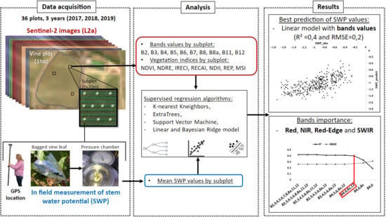
2. Materials and Methods
2.1. Data Acquisition
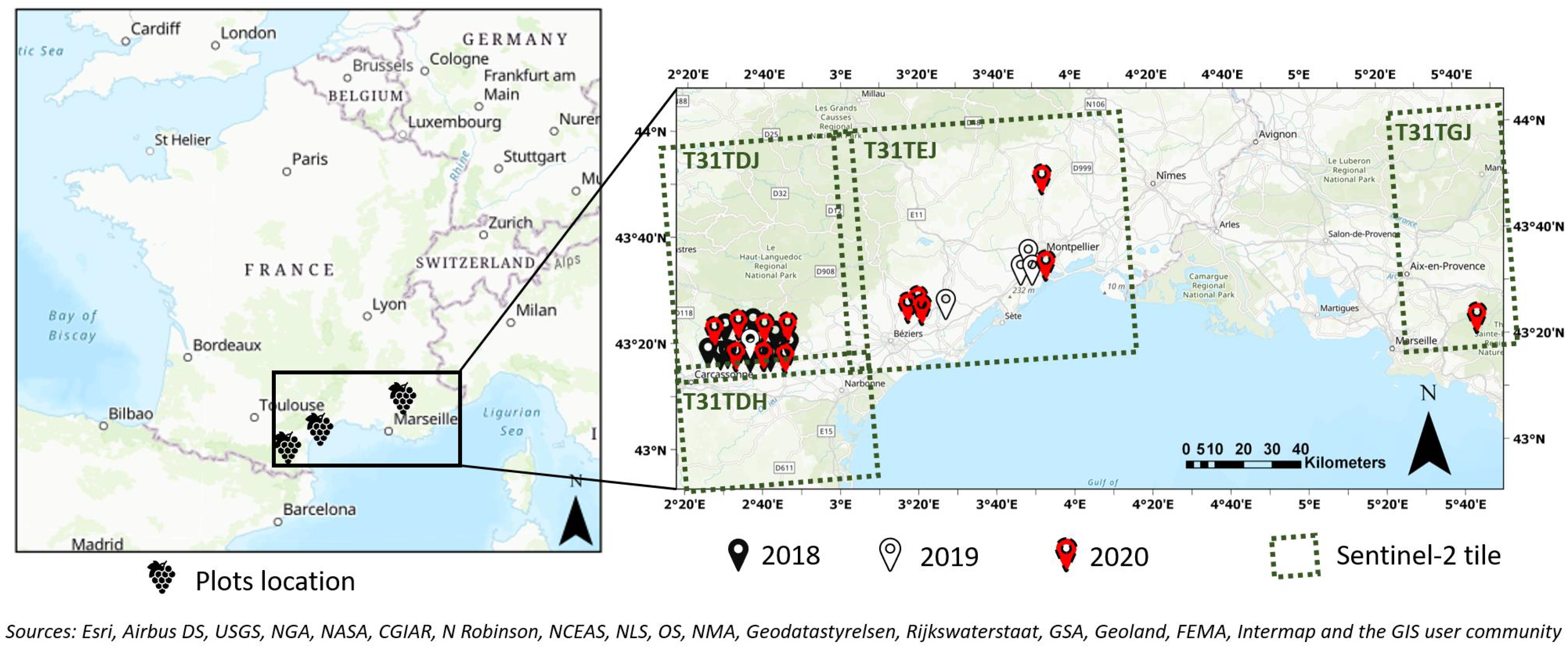
2.1.1. Study Sites
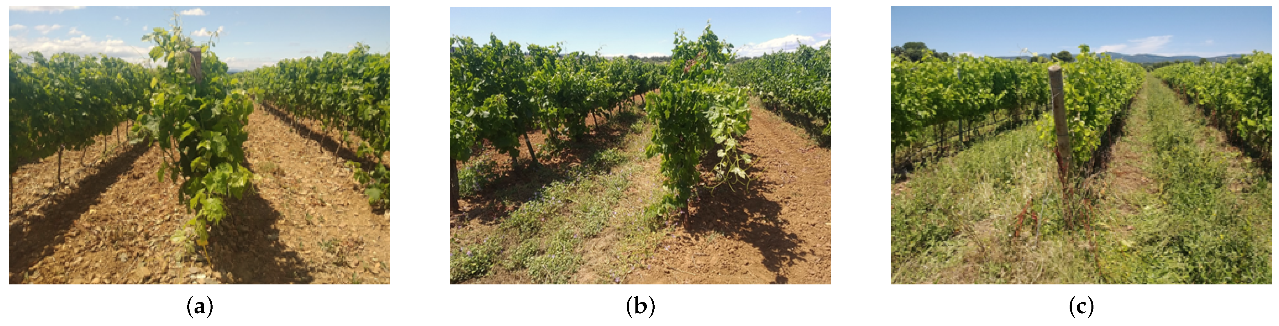
2.1.2. Experimental Design
2.1.3. Water Status
- Bagging mature leaves at 10 a.m. in order to close stomata and balance the sap pressure between plant and leaf;
- Removing leave with stem 3 or 4 h after, and set up quickly in the pressure chamber;
- Recording the pressure in MegaPascal (MPa) required to squeeze the first drop of sap out of the stem.
2.1.4. Sentinel-2 Images
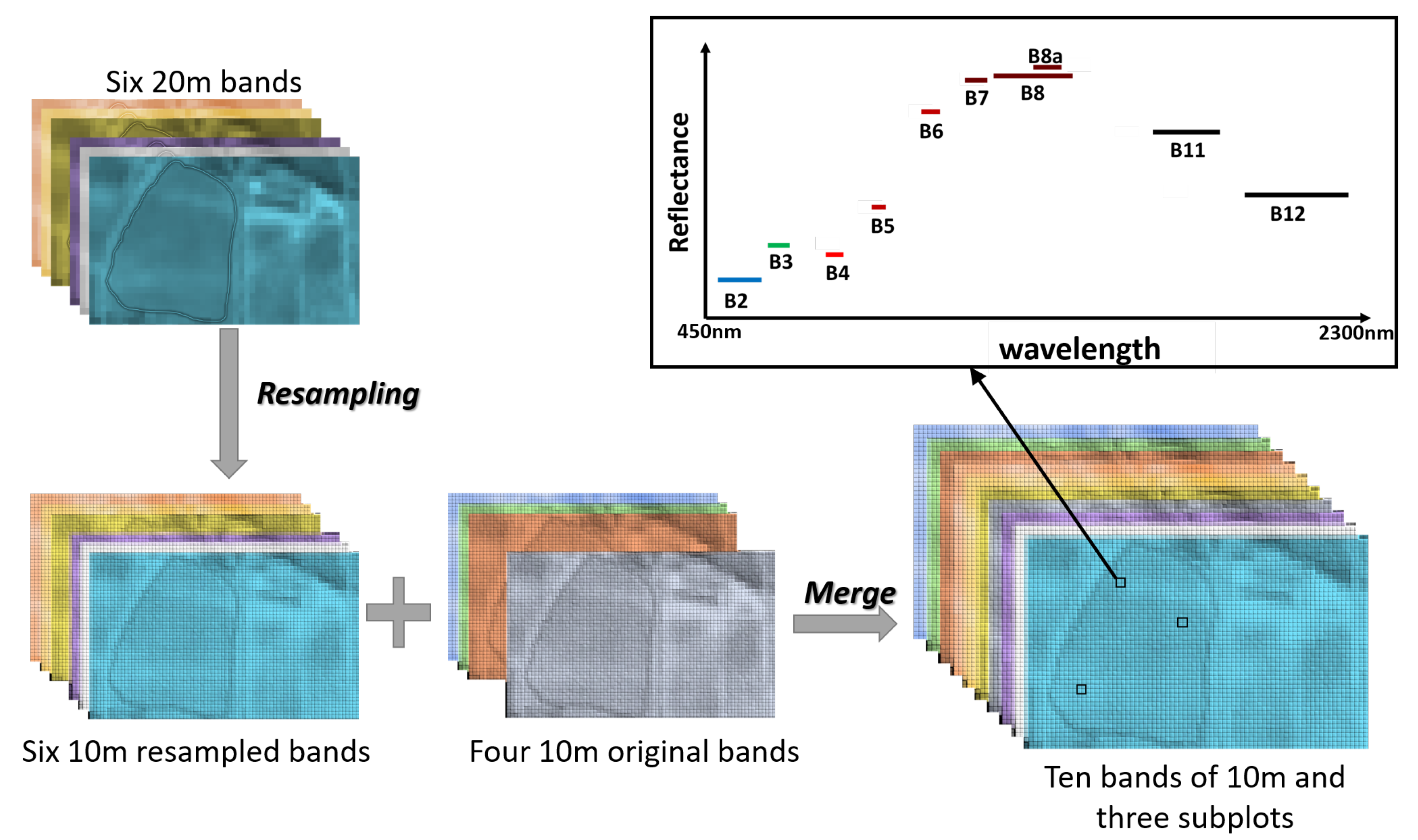
2.2. Sentinel-2 Images Preprocessing
2.3. Features Extraction
2.3.1. Sentinel-2 Reflectance Bands Values
2.3.2. Vegetation Indices
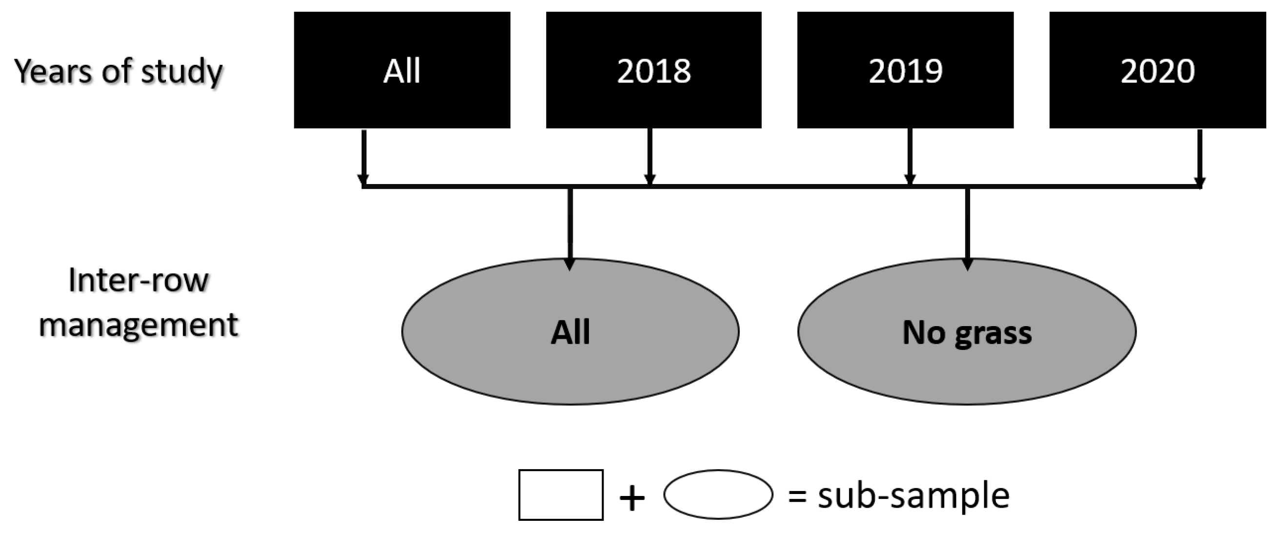
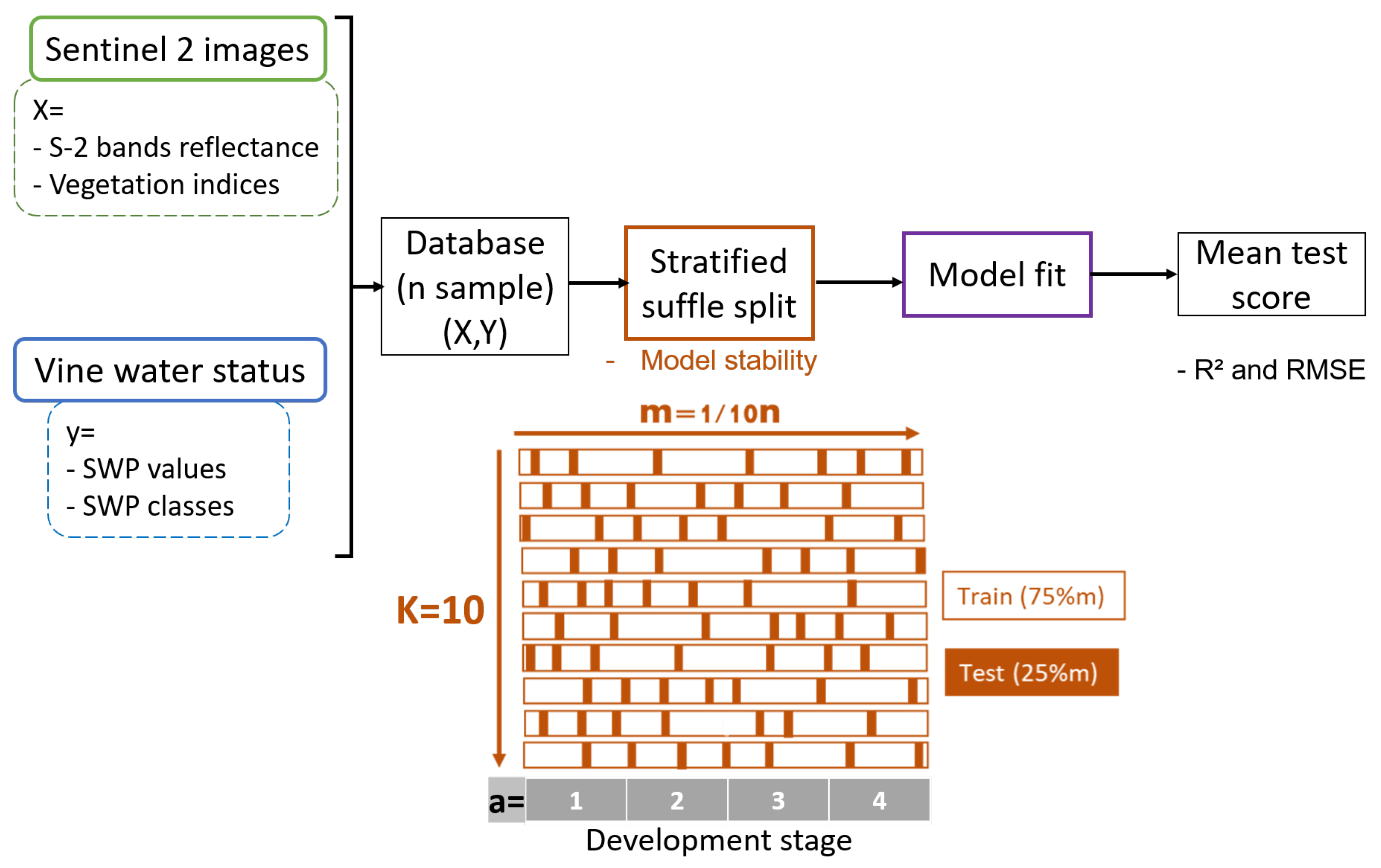
2.4. Analysis
2.4.1. SWP Mean by Subplot
2.4.2. Algorithms Description

| Name of the Algorithms | Type of the Algorithm | Reference |
|---|---|---|
| Kneighbors regressor | k-nearest neighbors | [45] |
| ExtraTrees regressor | Decision Tree | [46] |
| Support Vector Regressor | Support Vector Machine | [47] |
| Linear regression and BayesianRidge model | Linear Model | [48] |
2.4.3. Robustness and Precision Evaluation of Algorithms
- Regression score
2.4.4. Best Model Exploration
- Bands importance
- Impact of experimental conditions on the result
3. Results
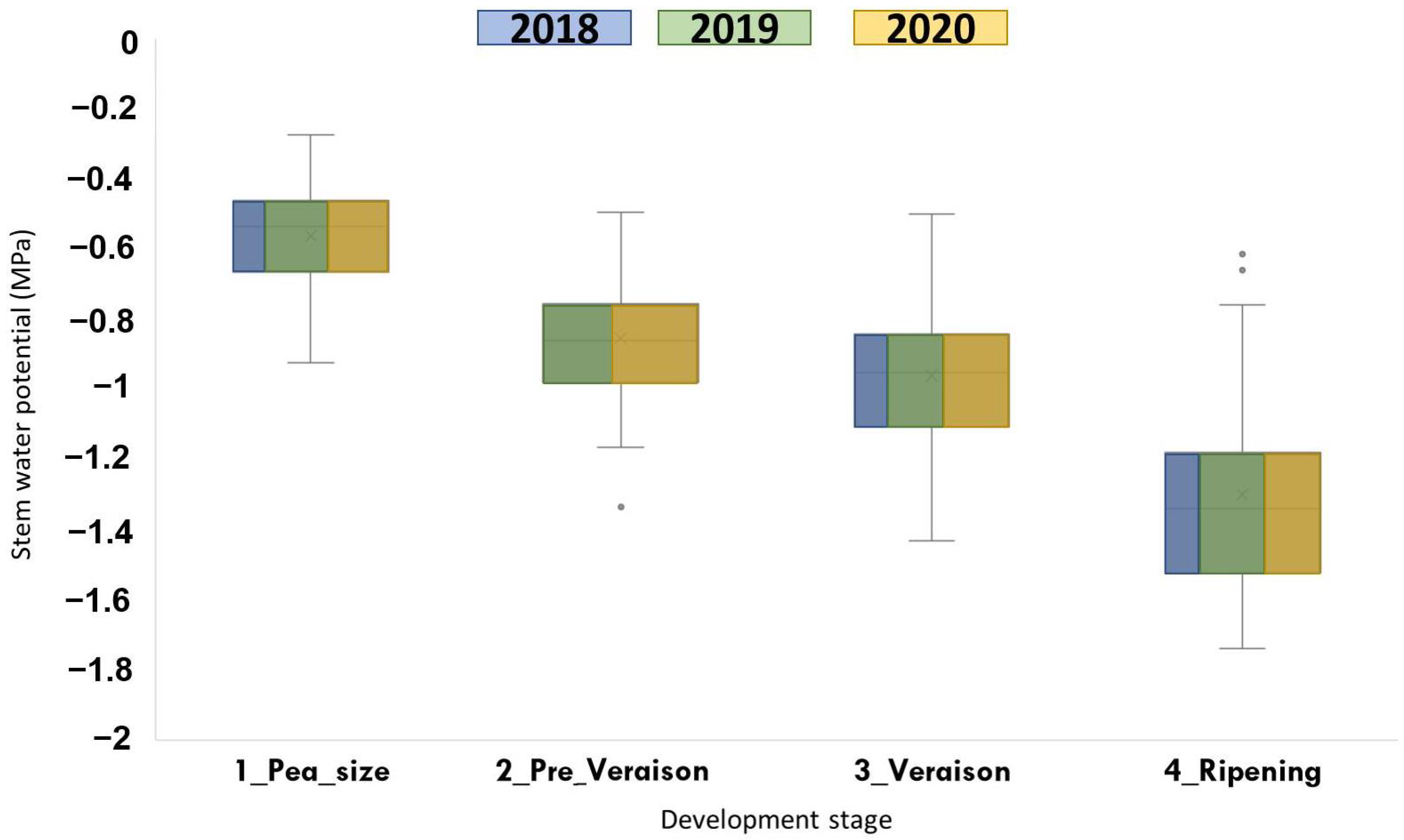
3.1. SWP Values
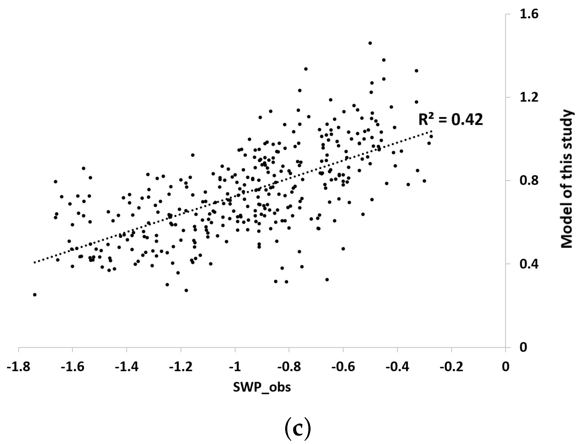
3.2. Evaluation of the Robustness and Precision
3.3. Best Models Exploration
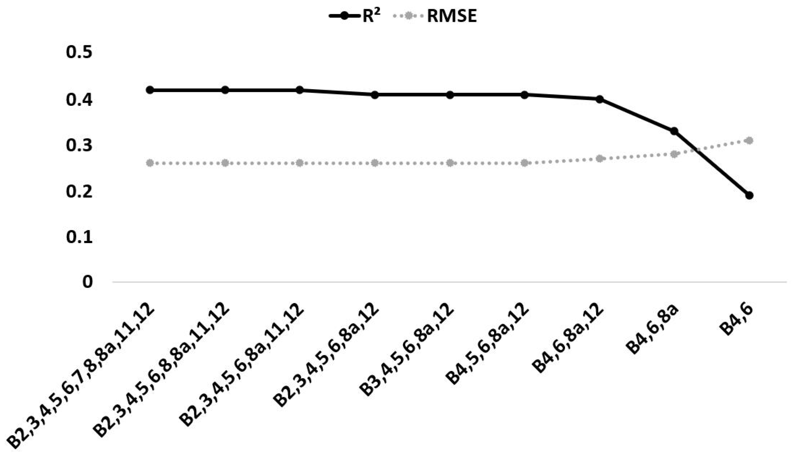
3.3.1. Bands Importance
3.3.2. Data Distribution and Impact of Experimental Conditions
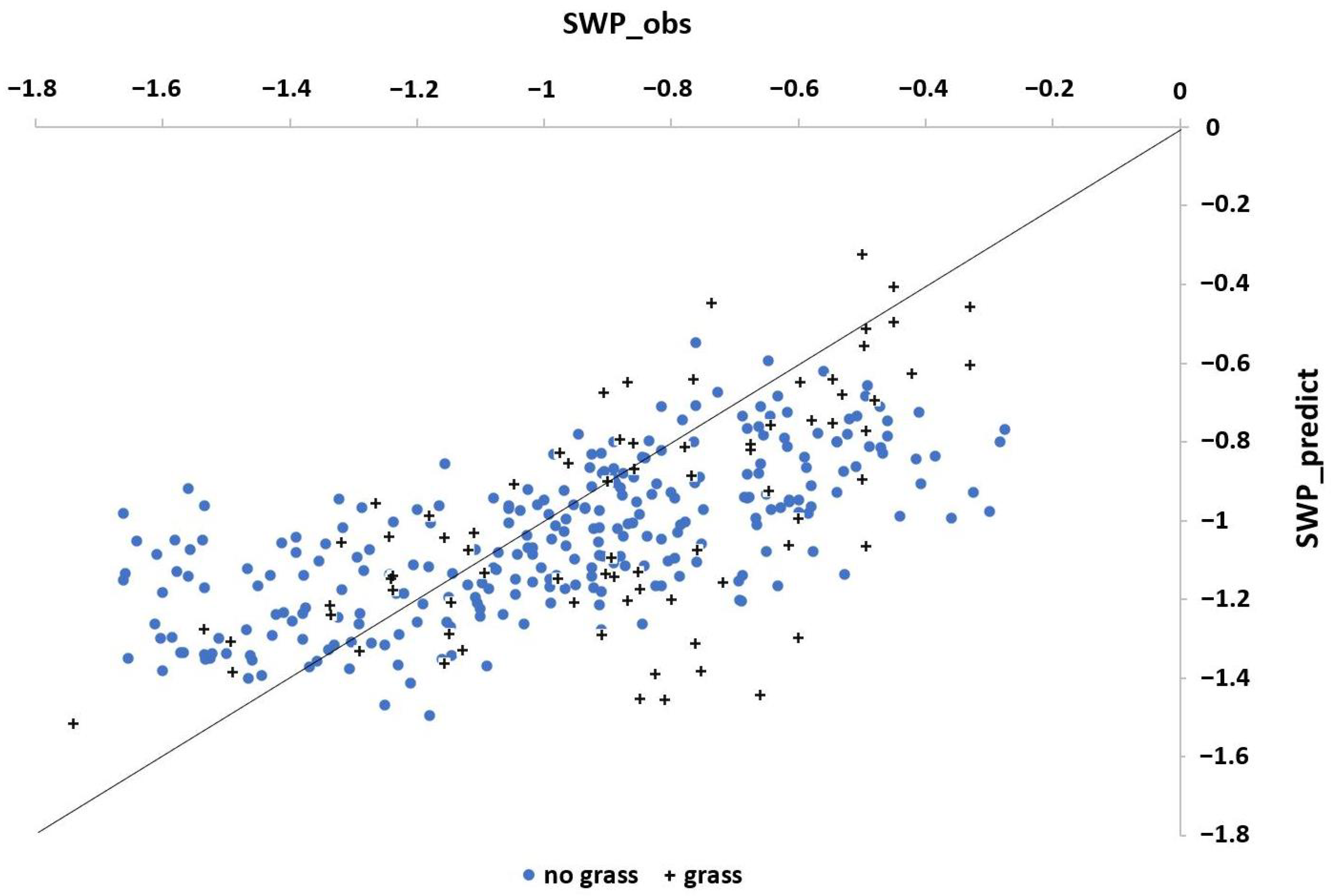
- Inter-row management
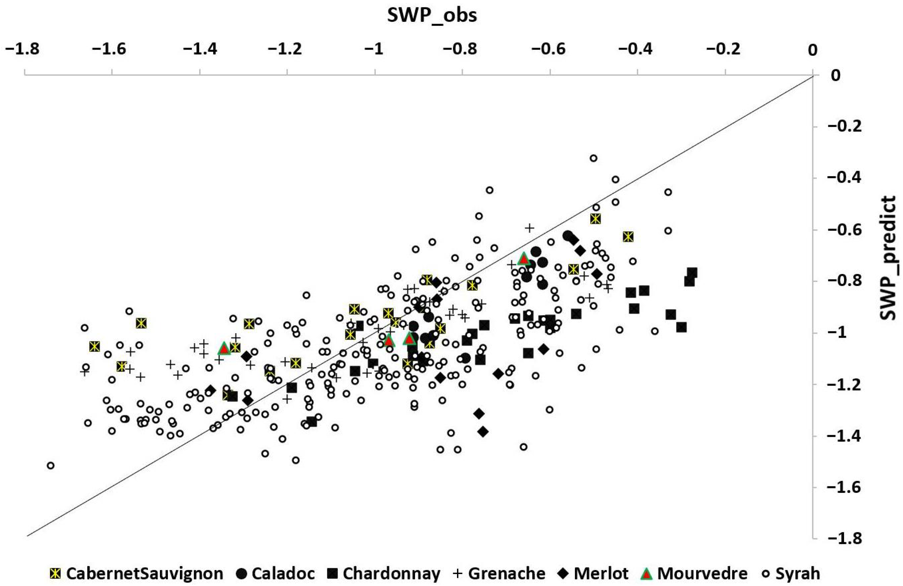
- Grape variety
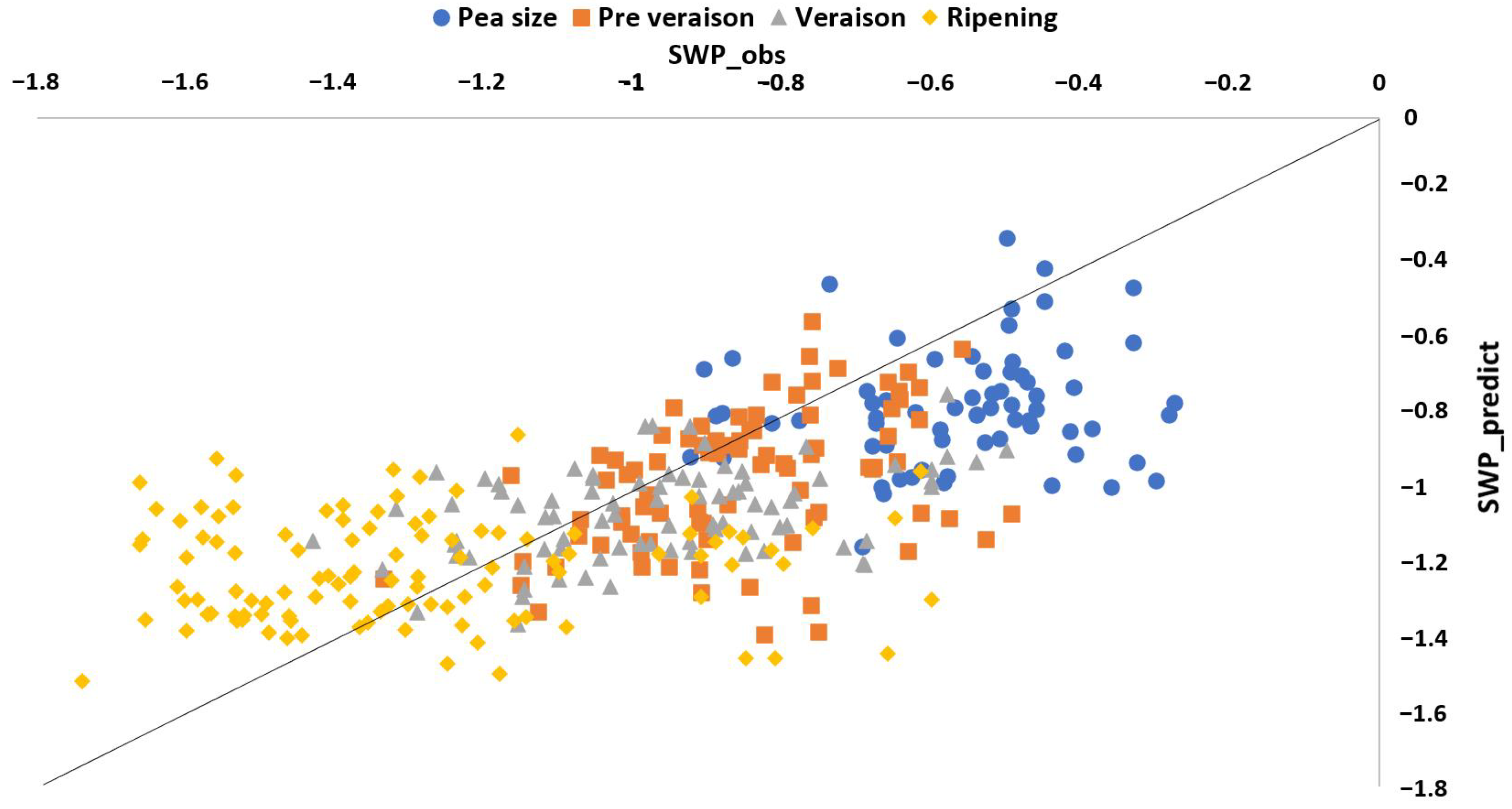
- Development stage
- Year of study
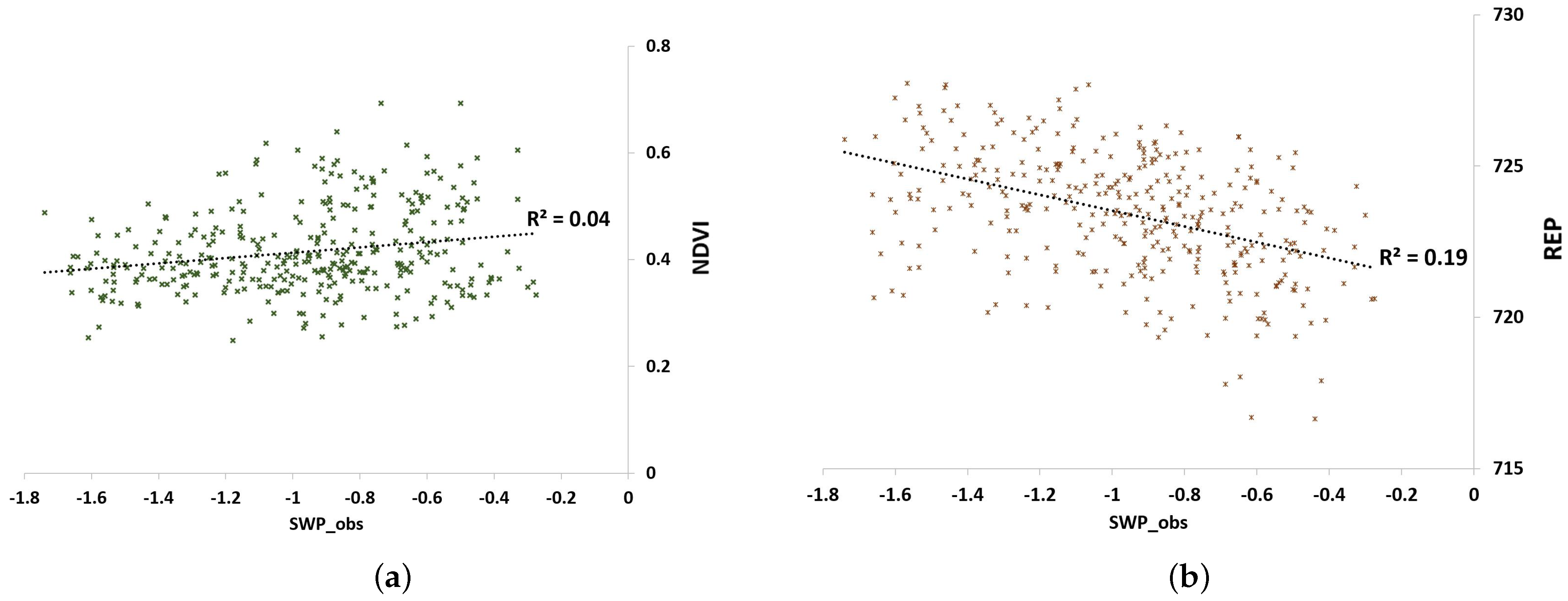
3.4. Comparison between NDVI, Best VI (REP) and Best Model with the Four S2 Bands
4. Discussion
4.1. Significant Features
4.2. Robustness of the Model
4.2.1. Impact of Grass Cover
4.2.2. Impact of Grape Variety
4.2.3. Impact of Development Stage
4.2.4. Impact of Years
4.3. Considerations for a Future Operational Service
- Avoid the pixels at the edge which can cover both the plot and a path or a forest bordering it for example. In order to avoid its so-called “mixed” pixels, an advice would be to apply a buffer around the edge of the plot of at least 5 m to keep and interpret only the pixels fully included in the plot,
- Be careful with the size and shape of the plot in order to have a consistent number of pixels to interpret inside the plot,
- Consider the inter-row management and the soil management and/or the soil composition which can impact the observed signal since vineyard is conducted in row and the inter-row is also visible with 10 or 20 m pixel. Maybe think to use two models according to the grass cover management (one for ungrassed field and one for grassed) by improving the number of grassed vine field in the database.
5. Conclusions
Author Contributions
Funding
Acknowledgments
Conflicts of Interest
Abbreviations
| MDPI | Multidisciplinary Digital Publishing Institute |
| DOAJ | Directory of open access journals |
| NIR | Near Infrared |
| NDVI | Normalized Difference Vegetation Index |
| S2 | Sentinel-2 |
| SWP | Stem Water Potential |
| SWIR | Short Wave Infra-Red |
| VI | Vegetation indices |
| REP | Red-Edge Position |
| RMSE | Root Mean Square Error |
References
- Ramos, M.C.; Pérez-Álvarez, E.P.; Peregrina, F.; Martínez de Toda, F. Relationships between grape composition of Tempranillo variety and available soil water and water stress under different weather conditions. Sci. Hortic. 2020, 262, 109063. [Google Scholar] [CrossRef]
- van Leeuwen, C.; Darriet, P. The Impact of Climate Change on Viticulture and Wine Quality. J. Wine Econ. 2016, 11, 150–167. [Google Scholar] [CrossRef] [Green Version]
- Chaves, M.; Santos, T.; Souza, C.; Ortuño, M.; Rodrigues, M.; Lopes, C.; Maroco, J.; Pereira, J. Deficit irrigation in grapevine improves water-use efficiency while controlling vigour and production quality. Ann. Appl. Biol. 2007, 150, 237–252. [Google Scholar] [CrossRef]
- Costa, J.M.; Ortuño, M.F.; Chaves, M.M. Deficit Irrigation as a Strategy to Save Water: Physiology and Potential Application to Horticulture. J. Integr. Plant Biol. 2007, 49, 1421–1434. [Google Scholar] [CrossRef]
- Gorguner, M.; Kavvas, M.L. Modeling impacts of future climate change on reservoir storages and irrigation water demands in a Mediterranean basin. Sci. Total Environ. 2020, 141246. [Google Scholar] [CrossRef] [PubMed]
- Medrano, H.; Tomás, M.; Martorell, S.; Escalona, J.M.; Pou, A.; Fuentes, S.; Flexas, J.; Bota, J. Improving water use efficiency of vineyards in semi-arid regions. A review. Agron. Sustain. Dev. 2015, 35, 499–517. [Google Scholar] [CrossRef] [Green Version]
- Bernardo, S.; Dinis, L.T.; Machado, N.; Moutinho-Pereira, J. Grapevine abiotic stress assessment and search for sustainable adaptation strategies in Mediterranean-like climates. A review. Agron. Sustain. Dev. 2018, 38. [Google Scholar] [CrossRef] [Green Version]
- Costa, J.M.; Vaz, M.; Escalona, J.; Egipto, R.; Lopes, C.; Medrano, H.; Chaves, M.M. Modern viticulture in southern Europe: Vulnerabilities and strategies for adaptation to water scarcity. Agric. Water Manag. 2016. [Google Scholar] [CrossRef]
- Addabbo, P.; Focareta, M.; Marcuccio, S.; Votto, C.; Ullo, S.L. Contribution of Sentinel-2 data for applications in vegetation monitoring. Acta Imeko 2016, 5, 44. [Google Scholar] [CrossRef]
- Segarra, J.; Buchaillot, M.L.; Araus, J.L.; Kefauver, S.C. Remote Sensing for Precision Agriculture: Sentinel-2 Improved Features and Applications. Agronomy 2020, 10, 641. [Google Scholar] [CrossRef]
- Devaux, N.; Crestey, T.; Leroux, C.; Tisseyre, B. Potential of Sentinel-2 satellite images to monitor vine fields grown at a territorial scale. OENO One 2019, 53, 51–58. [Google Scholar] [CrossRef]
- Di Gennaro, S.F.; Dainelli, R.; Palliotti, A.; Toscano, P.; Matese, A. Sentinel-2 validation for spatial variability assessment in overhead trellis system viticulture versus UAV and agronomic data. Remote Sens. 2019, 11, 2573. [Google Scholar] [CrossRef] [Green Version]
- Rozenstein, O.; Haymann, N.; Kaplan, G.; Tanny, J. Estimating cotton water consumption using a time series of Sentinel-2 imagery. Agric. Water Manag. 2018, 207, 44–52. [Google Scholar] [CrossRef]
- Cogato, A.; Pagay, V.; Marinello, F.; Meggio, F.; Grace, P.; De, M. Assessing the feasibility of using medium-resolution imagery information to quantify the impact of the heatwaves on irrigated vineyards. Remote Sens. 2019, 11, 2869. [Google Scholar] [CrossRef] [Green Version]
- Cohen, Y.; Gogumalla, P.; Bahat, I.; Netzer, Y.; Ben-Gal, A.; Lenski, I.; Michael, Y.; Helman, D. Can time series of multispectral satellite images be used to estimate stem water potential in vineyards. In Precision Agriculture ’19; Wageningen Academic: Wageningen, The Netherlands, 2019; pp. 445–451. [Google Scholar] [CrossRef]
- Seelig, H.D.; Hoehn, A.; Stodieck, L.S.; Klaus, D.M.; Adams, W.W.; Emery, W.J. The assessment of leaf water content using leaf reflectance ratios in the visible, near-, and short-wave-infrared. Int. J. Remote Sens. 2008, 29, 3701–3713. [Google Scholar] [CrossRef]
- Zovko, M.; Zibrat, U.; Knapic, M.; Bubalo Kovacic, M.; Romic, D. Hyperspectral remote sensing of grapevine drought stress. Precis. Agric. 2019, 20, 335–347. [Google Scholar] [CrossRef]
- Ceccato, P.; Flasse, S.; Tarantola, S.; Jacquemoud, S.; Grégoire, J.M. Detecting vegetation leaf water content using reflectance in the optical domain. Remote Sens. Environ. 2001, 77, 22–33. [Google Scholar] [CrossRef]
- Das, B.; Sahoo, R.N.; Pargal, S.; Krishna, G.; Verma, R.; Viswanathan, C.; Sehgal, V.K.; Gupta, V.K. Evaluation of different water absorption bands, indices and multivariate models for water-deficit stress monitoring in rice using visible-near infrared spectroscopy. Spectrochim. Acta Part A Mol. Biomol. Spectrosc. 2020, 119104. [Google Scholar] [CrossRef]
- Kim, D.; Zhang, H.; Zhou, H.; Du, T.; Wu, Q.; Mockler, T.; Berezin, M. Highly sensitive image-derived indices of water-stressed plants using hyperspectral imaging in SWIR and histogram analysis. Sci. Rep. 2015, 5, 15919. [Google Scholar] [CrossRef] [PubMed] [Green Version]
- Main, R.; Cho, M.A.; Mathieu, R.; O’Kennedy, M.M.; Ramoelo, A.; Koch, S. An investigation into robust spectral indices for leaf chlorophyll estimation. ISPRS J. Photogramm. Remote Sens. 2011, 66, 751–761. [Google Scholar] [CrossRef]
- Behmann, J.; Steinrücken, J.; Plümer, L. Detection of early plant stress responses in hyperspectral images. ISPRS J. Photogramm. Remote Sens. 2014, 93, 98–111. [Google Scholar] [CrossRef]
- Matese, A.; Di Gennaro, S.F. Technology in precision viticulture: A state of the art review. Int. J. Wine Res. 2015. [Google Scholar] [CrossRef] [Green Version]
- Tilling, A.K.; O’Leary, G.J.; Ferwerda, J.G.; Jones, S.D.; Fitzgerald, G.J.; Rodriguez, D.; Belford, R. Remote sensing of nitrogen and water stress in wheat. Field Crops Res. 2007, 104, 77–85. [Google Scholar] [CrossRef]
- Li, M.; Chu, R.; Yu, Q.; Islam, A.R.M.T.; Chou, S.; Shen, S. Evaluating Structural, Chlorophyll-Based and Photochemical Indices to Detect Summer Maize Responses to Continuous Water Stress. Water 2018, 10, 500. [Google Scholar] [CrossRef] [Green Version]
- Laroche-Pinel, E.; Albughdadi, M.; Duthoit, S.; Chéret, V.; Rousseau, J.; Clenet, H. Understanding Vine Hyperspectral Signature through Different Irrigation Plans: A First Step to Monitor Vineyard Water Status. Remote Sens. 2021, 13, 536. [Google Scholar] [CrossRef]
- Rouse, J.W.; Haas, R.H.; Schell, J.A.; Deering, D.W. Monitoring vegetation systems in the Great Plains with ERTS. In Third ERTS Symposium, NASA SP-351; NASA: Greenbelt, MD, USA, 1973; pp. 309–317. [Google Scholar]
- Rienth, M.; Scholasch, T. State-of-the-art of tools and methods to assess vine water status. OENO One 2019, 53, 619–637. [Google Scholar] [CrossRef]
- Romero, M.; Luo, Y.; Su, B.; Fuentes, S. Vineyard water status estimation using multispectral imagery from an UAV platform and machine learning algorithms for irrigation scheduling management. Comput. Electron. Agric. 2018, 147, 109–117. [Google Scholar] [CrossRef]
- Ferrant, S.; Selles, A.; Le Page, M.; Herrault, P.A.; Pelletier, C.; Al-Bitar, A.; Mermoz, S.; Gascoin, S.; Bouvet, A.; Saqalli, M.; et al. Detection of irrigated crops from Sentinel-1 and Sentinel-2 data to estimate seasonal groundwater use in South India. Remote Sens. 2017, 9, 1119. [Google Scholar] [CrossRef] [Green Version]
- Loggenberg, K.; Strever, A.; Greyling, B.; Poona, N. Modelling water stress in a Shiraz vineyard using hyperspectral imaging and machine learning. Remote Sens. 2018, 10, 202. [Google Scholar] [CrossRef] [Green Version]
- Schmitter, P.; Steinrücken, J.; Römer, C.; Ballvora, A.; Léon, J.; Rascher, U.; Plümer, L. Unsupervised domain adaptation for early detection of drought stress in hyperspectral images. ISPRS J. Photogramm. Remote Sens. 2017, 131, 65–76. [Google Scholar] [CrossRef]
- Conseil départemental de l’Hérault. Annales Climatologiques et Hydrologiques 2019; Technical Report; DREAL Occitanie; DREAL: Marseille, France, 2019. [Google Scholar]
- Conseil départemental de l’Hérault. Info Clim, Synthèse 2020; Technical Report 252; Conseil départemental de l’Hérault; DREAL: Marseille, France, 2020. [Google Scholar]
- Thales Alenia Space. Sentinel-2 Products Specification Document; Technical Report S2-PDGS-TAS-DI-PSD; ESA: Paris, France, 2016; Available online: https://sentinels.copernicus.eu/web/sentinel/document-library/latest-documents/-/asset_publisher/EgUy8pfXboLO/content/sentinel-2-level-1-to-level-1c-product-specifications;jsessionid=8BE6EE17FECEE9CDECD948BD1F6A8522.jvm2?redirect=https%3A%2F%2Fsentinels.copernicus.eu%2Fweb%2Fsentinel%2Fdocument-library%2Flatest-documents%3Bjsessionid%3D8BE6EE17FECEE9CDECD948BD1F6A8522.jvm2%3Fp_p_id%3D101_INSTANCE_EgUy8pfXboLO%26p_p_lifecycle%3D0%26p_p_state%3Dnormal%26p_p_mode%3Dview%26p_p_col_id%3Dcolumn-1%26p_p_col_pos%3D1%26p_p_col_count%3D2 (accessed on 10 April 2021).
- Donadieu, J.; L’Helguen, C. Sentinel-2A L2A Products Description; Technical Report PSC-NT-411-0362-CNES; CNES: Toulouse, France, 2016; Available online: https://labo.obs-mip.fr/wp-content-labo/uploads/sites/19/2016/09/PSC-NT-411-0362-CNES_01_00_SENTINEL-2A_L2A_Products_Description.pdf (accessed on 10 April 2021).
- Hagolle, O.; Huc, M.; Pascual, D.V.; Dedieu, G. A multi-temporal and multi-spectral method to estimate aerosol optical thickness over land, for the atmospheric correction of FormoSat-2, LandSat, VENμS and Sentinel-2 images. Remote Sens. 2015, 7, 2668–2691. [Google Scholar] [CrossRef] [Green Version]
- Baetens, L.; Desjardins, C.; Hagolle, O. Validation of copernicus Sentinel-2 cloud masks obtained from MAJA, Sen2Cor, and FMask processors using reference cloud masks generated with a supervised active learning procedure. Remote Sens. 2019, 11, 433. [Google Scholar] [CrossRef] [Green Version]
- ESA. Sentinel-2 Spectral Response Functions (S2-SRF); Technical Report COPE-GSEG-EOPG-TN-15-0007; ESA: Paris, France, 2017; Available online: https://sentinel.esa.int/web/sentinel/user-guides/sentinel-2-msi/document-library/-/asset_publisher/Wk0TKajiISaR/content/sentinel-2a-spectral-responses (accessed on 10 April 2021).
- Gitelson, A.A.; Viña, A.; Ciganda, V.; Rundquist, D.C.; Arkebauer, T.J. Remote estimation of canopy chlorophyll content in crops. Geophys. Res. Lett. 2005, 32, 1–4. [Google Scholar] [CrossRef] [Green Version]
- Frampton, W.J.; Dash, J.; Watmough, G.; Milton, E.J. Evaluating the capabilities of Sentinel-2 for quantitative estimation of biophysical variables in vegetation. ISPRS J. Photogramm. Remote Sens. 2013, 82, 83–92. [Google Scholar] [CrossRef] [Green Version]
- Cui, B.; Zhao, Q.; Huang, W.; Song, X.; Ye, H.; Zhou, X. A New Integrated Vegetation Index for the Estimation of Winter Wheat Leaf Chlorophyll Content. Remote Sens. 2019, 11, 974. [Google Scholar] [CrossRef] [Green Version]
- Lemaire, G.; Jeuffroy, M.H.; Gastal, F. Diagnosis tool for plant and crop N status in vegetative stage. Theory and practices for crop N management. Eur. J. Agron. 2008, 28, 614–624. [Google Scholar] [CrossRef]
- Pedregosa, F.; Varoquaux, G.; Gramfort, A.; Michel, V.; Thirion, B.; Grisel, O.; Blondel, M.; Prettenhofer, P.; Weiss, R.; Dubourg, V.; et al. Scikit-learn: Machine Learning in Python. J. Mach. Learn. Res. 2011, 12, 2825–2830. [Google Scholar]
- Kramer, O. K-Nearest Neighbors. In Dimensionality Reduction with Unsupervised Nearest Neighbors; Springer: Berlin/Heidelberg, Germany, 2013; pp. 13–23. [Google Scholar] [CrossRef]
- Kazemitabar, J.; Amini, A.; Bloniarz, A.; Talwalkar, A.S. Variable Importance Using Decision Trees. In Advances in Neural Information Processing Systems 30; Guyon, I., Luxburg, U.V., Bengio, S., Wallach, H., Fergus, R., Vishwanathan, S., Garnett, R., Eds.; Curran Associates Inc.: Greenbelt, MD, USA, 2017; pp. 426–435. [Google Scholar]
- Awad, M.; Khanna, R. Support Vector Regression. In Efficient Learning Machines: Theories, Concepts, and Applications for Engineers and System Designers; Apress: Berkeley, CA, USA, 2015; pp. 67–80. [Google Scholar] [CrossRef] [Green Version]
- Pilz, J. Bayesian estimation and experimental design in linear regression models. J. Am. Stat. Assoc. 1992, 87, 1250. [Google Scholar]
- Ballester, C.; Zarco-Tejada, P.J.; Nicolás, E.; Alarcón, J.J.; Fereres, E.; Intrigliolo, D.S.; Gonzalez-Dugo, V. Evaluating the performance of xanthophyll, chlorophyll and structure-sensitive spectral indices to detect water stress in five fruit tree species. Precis. Agric. 2017, 1–16. [Google Scholar] [CrossRef]
- Maimaitiyiming, M.; Ghulam, A.; Bozzolo, A.; Wilkins, J.L.; Kwasniewski, M.T. Early detection of plant physiological responses to different levels of water stress using reflectance spectroscopy. Remote Sens. 2017, 9, 745. [Google Scholar] [CrossRef] [Green Version]
- Das, B.; Mahajan, G.R.; Singh, R. Hyperspectral Remote Sensing: Use in Detecting Abiotic Stresses in Agriculture. Adv. Crop. Environ. Interact. 2018, 317–335. [Google Scholar] [CrossRef]
- Rapaport, T.; Hochberg, U.; Shoshany, M.; Karnieli, A.; Rachmilevitch, S. Combining leaf physiology, hyperspectral imaging and partial least squares-regression (PLS-R) for grapevine water status assessment. ISPRS J. Photogramm. Remote Sens. 2015, 109, 88–97. [Google Scholar] [CrossRef]
- Ojeda, H.; Saurin, N. L’irrigation de précision de la vigne: Méthodes, outils et stratégies pour maximiser la qualité et les rendements de la vendange en économisant de l’eau. Innov. Agron. 2014, 38, 97–108. [Google Scholar]
- Simonneau, T.; Ollat, N.; Pellegrino, A.; Lebon, E. Contrôle de l’état hydrique dans la plante et réponses physiologiques de la vigne à la contrainte hydrique. Innov. Agron. 2014, 38, 13–82. [Google Scholar]
- Suter, B.; Destrac Irvine, A.; Gowdy, M.; Dai, Z.; van Leeuwen, C. Adapting Wine Grape Ripening to Global Change Requires a Multi-Trait Approach. Front. Plant Sci. 2021, 12, 1–17. [Google Scholar] [CrossRef] [PubMed]


| Year | Month | Rainfall | Temperatures | Events |
|---|---|---|---|---|
| May | Very excessive | Alternating hot and very cold | Thunderstorms, hail and snow | |
| June | Very excessive | In accordance with season | ||
| 2018 | July | No rainfall | Mild to warm | |
| August | Normal | Very hot | Storms, heatwave the first week | |
| September | Very low | Very hot | ||
| May | Deficit | Cool to very cool | ||
| June | Deficit | Average to cool | Heatwave from the 26th to the 28th | |
| 2019 | July | Deficit | Very hot | Heatwave, hail and fire |
| August | Deficit | Hot to very hot | ||
| September | Constrasting | Warm to very warm | ||
| May | Heterogeneous | Mild to hot | ||
| June | Heterogeneous | Cool, warm the last week | ||
| 2020 | July | Poor | Warm to hot | Hail and fires |
| August | Heterogeneous | Warm | ||
| September | Heterogeneous | Warm |
| 2018 | 2019 | 2020 | Total | |||||
|---|---|---|---|---|---|---|---|---|
| Plot | Subplot | Plot | Subplot | Plot | Subplot | Plot | Subplot | |
| Total | 11 | 18 | 5 | 32 | 20 | 53 | 36 | 103 |
| Inter-row management | ||||||||
| Grass | 4 | 7 | 0 | 0 | 8 | 20 | 12 | 27 |
| No grass | 7 | 11 | 5 | 32 | 12 | 33 | 24 | 76 |
| Grape Variety | ||||||||
| Syrah | 11 | 18 | 3 | 19 | 7 | 18 | 21 | 55 |
| Grenache | 0 | 0 | 1 | 6 | 1 | 2 | 2 | 8 |
| Chardonnay | 0 | 0 | 1 | 7 | 0 | 0 | 1 | 7 |
| Merlot | 0 | 0 | 0 | 0 | 1 | 3 | 1 | 3 |
| Cabernet Sauvignon | 0 | 0 | 0 | 0 | 2 | 5 | 2 | 5 |
| Caladoc | 0 | 0 | 0 | 0 | 1 | 6 | 1 | 6 |
| Mourvèdre | 0 | 0 | 0 | 0 | 1 | 1 | 1 | 1 |
| Band | Spectral Region | Wavelength Range (nm) | Spatial Resolution |
|---|---|---|---|
| B2 | Blue | 458–523 | 10 m |
| B3 | Green | 543–578 | 10 m |
| B4 | Red | 650–680 | 10 m |
| B5 | Red-Edge 1 | 698–713 | 20 m |
| B6 | Red-Edge 2 | 733–748 | 20 m |
| B7 | Near Infrared | 779–793 | 20 m |
| B8 | Near Infrared | 785–899 | 10 m |
| B8a | Near Infrared | 855–875 | 20 m |
| B11 | Shortwave Infrared | 1565–1655 | 20 m |
| B12 | Shortwave Infrared | 2100–2280 | 20 m |
| S2 Tile | Year of Study | June | July | August | September |
|---|---|---|---|---|---|
| 2018 | 27th and 30th | 30th | 1st | 8th and 10th | |
| T31TDH/TDJ | 2019 | 17th | 5th, 17th and 25th | 14th | |
| 2020 | 19th and 21st | 1st, 4th, 16th and 29th | 10th, 15th and 25th | ||
| T31TEJ | 2019 | 17th and 22nd | 2nd and 17th | 16th and 26th | |
| 2020 | 16th and 26th | 6th, 11th, 16th, 26th and 31st | 10th, 15th and 25th | ||
| T31TGJ | 2020 | 28th | 2nd |
| Index (Abbreviation) | Main Use | Formula Used with S2 Bands | Reference |
|---|---|---|---|
| Normalized Difference Vegetation Index (NDVI) | Vigor | [27] | |
| Normalized Difference Red-Edge (NDRE 1/2) | Chlorophyll, Water | [40] | |
| Inverted Red-Edge Chlorophyll Index (IRECI) | Chlorophyll | [41] | |
| Red-Edge Chlorophyll Absorption Index (RECAI) | Chlorophyll | [42] | |
| Normalized Difference Infrared Index (NDII) | Chlorophyll, Water | [43] | |
| Red-Edge Position (REP) | Chlorophyll | [21] | |
| Moisture Stress Index (MSI) | Water | [18] |
| Years | 2018 | 2019 | 2020 | ||||||||
|---|---|---|---|---|---|---|---|---|---|---|---|
| Development Stage | 1 | 3 | 4 | 1 | 2 | 3 | 4 | 1 | 2 | 3 | 4 |
| Nb_observation | 15 | 17 | 18 | 26 | 39 | 32 | 49 | 27 | 48 | 37 | 41 |
| Min | −0.68 | −1.27 | −1.74 | −0.93 | −1.17 | −1.15 | −1.66 | −0.91 | −1.34 | −1.43 | −1.66 |
| Max | −0.33 | −0.50 | −0.60 | −0.28 | −0.53 | −0.54 | −0.62 | −0.42 | −0.49 | −0.72 | −0.80 |
| Median | −0.46 | −0.91 | −1.20 | −0.52 | −0.92 | −0.92 | −1.41 | −0.63 | −0.81 | −1.09 | −1.32 |
| Mean | −0.47 | −0.87 | −1.14 | −0.55 | −0.91 | −0.89 | −1.34 | −0.63 | −0.81 | −1.06 | −1.31 |
| STD | 0.09 | 0.21 | 0.28 | 0.18 | 0.16 | 0.16 | 0.25 | 0.13 | 0.15 | 0.18 | 0.25 |
| Algorithms | ||||||
|---|---|---|---|---|---|---|
| Features | Scores | K-Nearest Kneighbors | ExtraTrees | Support Vector | Linear Model | Bayesian Model |
| All S2 bands | R2 | 0.29 | 0.39 | 0.37 | 0.40 | 0.40 |
| RMSE | 0.28 | 0.26 | 0.26 | 0.26 | 0.26 | |
| NDVI | R2 | 0.03 | 0.03 | 0.03 | 0.04 | 0.04 |
| RMSE | 0.34 | 0.39 | 0.33 | 0.33 | 0.33 | |
| NDRE1 | R2 | 0.07 | 0.05 | 0.03 | 0.004 | 0.003 |
| RMSE | 0.34 | 0.41 | 0.33 | 0.33 | 0.33 | |
| NDRE2 | R2 | 0.14 | 0.06 | 0.02 | 0.04 | 0.04 |
| RMSE | 0.35 | 0.42 | 0.33 | 0.33 | 0.33 | |
| IRECI | R2 | 0.02 | 0.04 | 0.11 | 0.11 | 0.11 |
| RMSE | 0.34 | 0.39 | 0.31 | 0.31 | 0.31 | |
| RECAI | R2 | 0.02 | 0.04 | 0.02 | 0.02 | 0.01 |
| RMSE | 0.36 | 0.33 | 0.34 | 0.34 | 0.33 | |
| NDII | R2 | 0.04 | 0.05 | 0.07 | 0.09 | 0.09 |
| RMSE | 0.34 | 0.41 | 0.32 | 0.32 | 0.32 | |
| REP | R2 | 0.02 | 0.03 | 0.15 | 0.19 | 0.17 |
| RMSE | 0.33 | 0.39 | 0.31 | 0.30 | 0.30 | |
| MSI | R2 | 0.09 | 0.06 | 0.07 | 0.10 | 0.10 |
| RMSE | 0.34 | 0.41 | 0.31 | 0.31 | 0.31 | |
| Year | Inter-Row Management | REP | All S2 Bands |
|---|---|---|---|
| All | All | < 0.25 | = 0.40 RMSE = 0.26 Bayesian Ridge model and Linear model |
| No grass | < 0.25 | = 0.48 RMSE = 0.24 Linear model | |
| 2018 | All | < 0.25 | < 0.25 |
| No grass | < 0.25 | = 0.52 RMSE = 0.2 Extra Tree regressor | |
| 2019 | No grass | = 0.27 RMSE = 0.29 Bayesian Ridge model | = 0.58 RMSE = 0.22 Linear model |
| 2020 | All | < 0.25 | = 0.48 RMSE = 0.21 Bayesian Ridge model and Linear model |
| No grass | < 0.25 | = 0.56 RMSE = 0.21 Bayesian Ridge Model |
Publisher’s Note: MDPI stays neutral with regard to jurisdictional claims in published maps and institutional affiliations. |
© 2021 by the authors. Licensee MDPI, Basel, Switzerland. This article is an open access article distributed under the terms and conditions of the Creative Commons Attribution (CC BY) license (https://creativecommons.org/licenses/by/4.0/).
Share and Cite
Laroche-Pinel, E.; Duthoit, S.; Albughdadi, M.; Costard, A.D.; Rousseau, J.; Chéret, V.; Clenet, H. Towards Vine Water Status Monitoring on a Large Scale Using Sentinel-2 Images. Remote Sens. 2021, 13, 1837. https://0-doi-org.brum.beds.ac.uk/10.3390/rs13091837
Laroche-Pinel E, Duthoit S, Albughdadi M, Costard AD, Rousseau J, Chéret V, Clenet H. Towards Vine Water Status Monitoring on a Large Scale Using Sentinel-2 Images. Remote Sensing. 2021; 13(9):1837. https://0-doi-org.brum.beds.ac.uk/10.3390/rs13091837
Chicago/Turabian StyleLaroche-Pinel, Eve, Sylvie Duthoit, Mohanad Albughdadi, Anne D. Costard, Jacques Rousseau, Véronique Chéret, and Harold Clenet. 2021. "Towards Vine Water Status Monitoring on a Large Scale Using Sentinel-2 Images" Remote Sensing 13, no. 9: 1837. https://0-doi-org.brum.beds.ac.uk/10.3390/rs13091837