Article

Comparing PlanetScope to Landsat-8 and Sentinel-2 for Sensing Water Quality in Reservoirs in Agricultural Watersheds

by
Abubakarr S. Mansaray
1,*,
Andrew R. Dzialowski
2,
Meghan E. Martin
3,
Kevin L. Wagner
1,
Hamed Gholizadeh
4 and
Scott H. Stoodley
3
1
Oklahoma Water Resources Center, Division of Agricultural Sciences and Natural Resources, Ferguson College of Agriculture, Oklahoma State University, Stillwater, OK 74078, USA
2
Department of Integrative Biology, Oklahoma State University, Stillwater, OK 74078, USA
3
Environmental Science Graduate Program, Oklahoma State University, Stillwater, OK 74078, USA
4
Department of Geography, Oklahoma State University, Stillwater, OK 74078, USA
*
Author to whom correspondence should be addressed.
Submission received: 15 March 2021 / Revised: 4 May 2021 / Accepted: 5 May 2021 / Published: 9 May 2021
(This article belongs to the Special Issue Remote Sensing for Water Resources Assessment in Agriculture)

Abstract

:
Agricultural runoff transports sediments and nutrients that deteriorate water quality erratically, posing a challenge to ground-based monitoring. Satellites provide data at spatial-temporal scales that can be used for water quality monitoring. PlanetScope nanosatellites have spatial (3 m) and temporal (daily) resolutions that may help improve water quality monitoring compared to coarser-resolution satellites. This work compared PlanetScope to Landsat-8 and Sentinel-2 in their ability to detect key water quality parameters. Spectral bands of each satellite were regressed against chlorophyll a, turbidity, and Secchi depth data from 13 reservoirs in Oklahoma over three years (2017–2020). We developed significant regression models for each satellite. Landsat-8 and Sentinel-2 explained more variation in chlorophyll a than PlanetScope, likely because they have more spectral bands. PlanetScope and Sentinel-2 explained relatively similar amounts of variations in turbidity and Secchi Disk data, while Landsat-8 explained less variation in these parameters. Since PlanetScope is a commercial satellite, its application may be limited to cases where the application of coarser-resolution satellites is not feasible. We identified scenarios where PS may be more beneficial than Landsat-8 and Sentinel-2. These include measuring water quality parameters that vary daily, in small ponds and narrow coves of reservoirs, and at reservoir edges.

1. Introduction

Agricultural runoff transports sediments and nutrients to downstream ecosystems where they may cause major water quality impairments. Sediments in the runoff cause elevation in turbidity (Turb) and a cascade of water quality problems such as a reduction in light penetration, low ecological productivity, alteration of food chains, and bioavailability of associated pollutants [1]. Nutrients brought in by the runoff can stimulate phytoplankton growth and promote harmful algal blooms (HABs) in downstream lakes and reservoirs [2]. A major problem with changes in water clarity and phytoplankton growth is that they are both spatially and temporally erratic.
The erratic nature of chlorophyll a (Chl-a) is evident in surface algal blooms, which may occur or disappear within hours or days depending on the underlying processes in a water body [3]. Algal blooms may be more frequent when nutrient loading through sediment transport is persistent. Since agricultural watersheds transport nutrients to lakes and reservoirs, especially during high flows, daily monitoring of sediments and phytoplankton in reservoirs may be the best way to detect pollution at the early stage of impairment.
Successful water quality monitoring programs require the collection of data that capture spatial and temporal trends in many water bodies [4,5]. Achieving this is often challenging because of limited resources. Many water bodies are not frequently monitored, resulting in uncertainties in determining if they support their beneficial uses and the magnitude to which they are impacted by nutrients and sediments [6]. Water quality monitoring programs often utilize rotational monitoring schedules to address this issue. The problem with infrequent monitoring and determining which water bodies to include in a rotational monitoring program is the possibility of missing out on significant pollution events because of their high temporal and spatial variations [7].
The availability of remotely sensed data from satellites provides the opportunity to monitor water bodies at greater temporal and spatial resolutions than field-based monitoring alone [8]. Studies have developed various methods to use spectral bands for water quality sensing. Examples include band ratios and band indices [9,10], spectral derivative techniques [11], and color space transformation [12]. The resulting spectral data are paired with the temporally and spatially coincident water quality data to establish empirical or analytical relationships [13]. Three key water quality parameters that have been studied using satellite remote sensing are Chl-a, Turb, and Secchi Disk depth (SD).
Satellite remote sensing of Chl-a is an active area of research because Chl-a is associated with adverse ecological effects at high concentrations during bloom events [14], and it is optically active with spectral signatures of green (G) reflectance and absorbance in red (R) and blue (B) [15]. The optical properties of Chl-a have been used to develop several empirical models using spectral bands and band combinations. For example, a ratio of R to near-infrared (NIR) is a common band ratio used to estimate Chl-a concentrations [9,16,17,18]. Other examples of band combinations used to monitor Chl-a in water bodies include a ratio of B to G [19] and the normalized difference between NIR and R at specific wavelengths [10]. First and second derivatives have also been used to study Chl-a in waterbodies. Becker et al. (2005) defined the first and second derivatives as shown in Equations 1 and 2, respectively.
d1st = (ρn+1 − ρn)/(λn+1 − λn)
d2nd = (dn+11st − dn1st)/(λn+2 − λn)
where d1st and d2nd are the first and second derivatives, n is the band number, ρ is the surface reflectance, and λ is the wavelength.
Similarly, studies have used both single bands, such as B and R, and band combinations, such as B/R and G/R, to study SD and Turb [20,21]. Polynomial terms of single bands, such as R3, have also been used [22]. Studies have also compared visible bands from different satellite sensors to estimate water transparency [23].
Remotely sensed data from satellites with moderate to coarse spatial resolution imagery such as Landsat-8 (with a spatial resolution of 30 m) and the Sentinel-2 constellation (with a spatial resolution ranging from 10 to 60 m) have shown promising results in monitoring water quality in inland water bodies [24,25]. However, their applications for remotely sensing water quality in small reservoirs, narrow coves of large reservoirs, or for parameters such as Chl-a that can vary daily within a system may be limited. PlanetScope (PS) is a relatively new satellite that provides greater temporal (daily repeat schedule) and spatial (3 m) resolution than these other satellites (Table 1). The temporal resolution of Landsat-8 is 16 days and for Sentinel-2 is 10 days for each of its two polar-orbiting satellites giving an average temporal resolution of 5 days. [26]. Table 1 compares some of the major characteristics of PS, Landsat-8, and Sentinel-2. As such, we posit that where adequate characterization of water quality for small reservoirs using moderate-coarse resolution data (e.g., Landsat-8, Sentinel-2) might not be feasible, PS data with finer spatial (3 m) and temporal (daily) resolutions may be a viable alternative.
The spatial and temporal resolutions of PS for water resource remote sensing are promising as shown in recent studies including bathymetric mapping [27] and change detection of water quality parameters such as total suspended matter [28]. PS imagery produced up to 50% overall accuracy for mapping benthic habitats with multiple species, including coral reefs, macroalgae, seagrass, bare substratum, and dead coral. Up to 74.31% accuracy was recorded for mapping several species of seagrass [29]. PS has also been used together with Landsat-8 to improve on bathymetric maps produced by Landsat-8 [30].
The advantage of PS for water quality sensing in comparison to Landsat-8 and Sentinel-2 may be limited by the number of spectral bands. Landsat-8 and Sentinel-2 have additional spectral bands that may give them an advantage over PS to remotely sense water quality. The shortwave infrared (SWIR) bands have been shown to be less susceptible to Turb than the NIR band and, hence, better detect Chl-a [31]. The Red-Edge band in Sentinel-2 has also been shown to better detect Chl-a than the NIR band [32].
The objective of this study was to determine if the finer spatial and temporal resolutions of PS provided better water quality monitoring potential compared to Landsat-8 and Sentinel-2. To achieve this, we determined empirical relationships between the surface reflectance of each of the three satellites and Chl-a, Turb, and SD data from 13 reservoirs in Oklahoma. We also present a specific case study of an algal bloom in an Oklahoma reservoir to compare the utility of the three satellite platforms in monitoring an algal bloom with respect to the spatial, temporal, and spectral properties of each satellite.

2. Materials and Methods

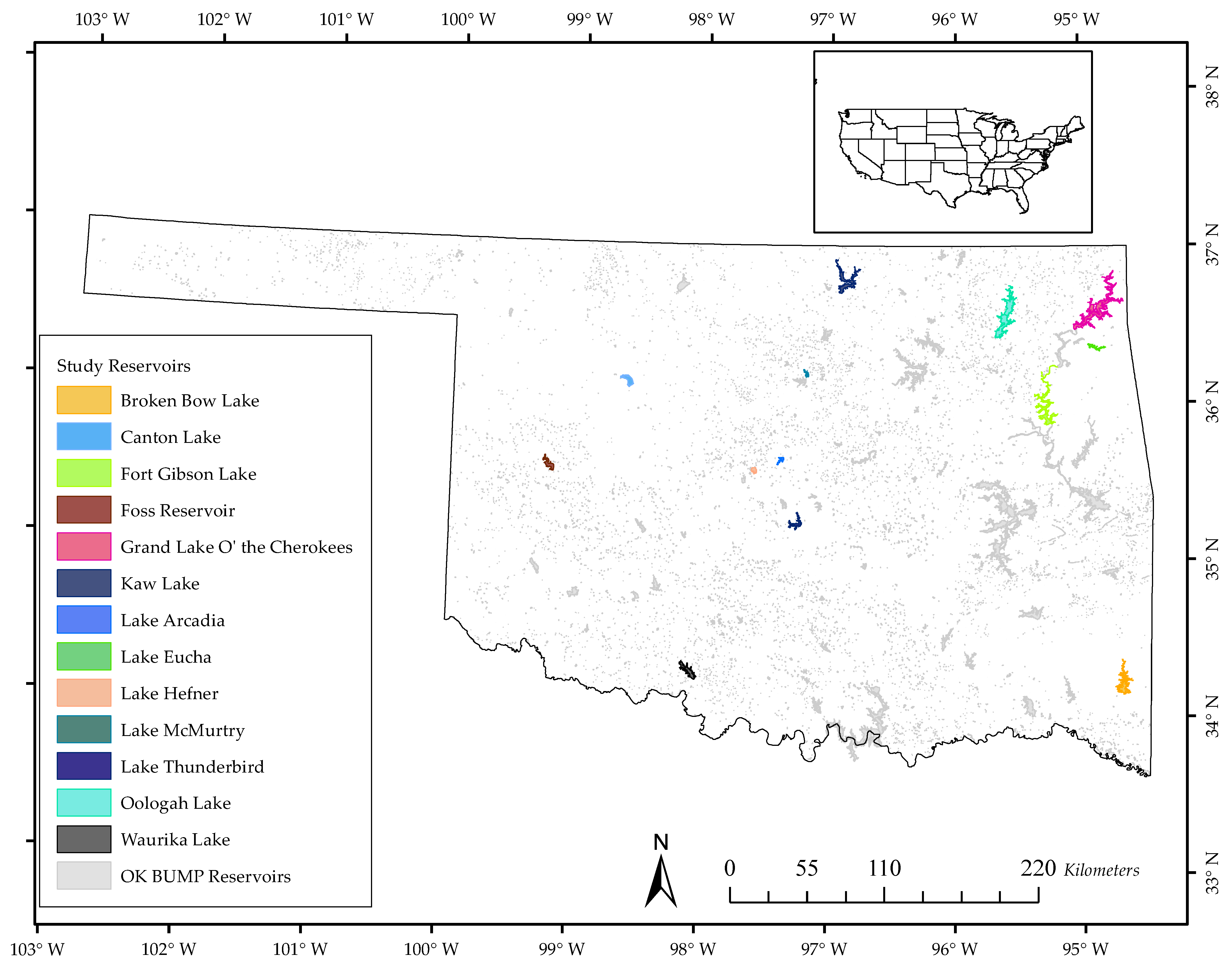
2.1. Description of the Study Area

The state of Oklahoma has a total surface area of 181,196 km2. It has approximately 3629 km2 of water in reservoirs and ponds and 89,554 km of shoreline [33]. There are over 200 reservoirs distributed across the state that are greater than 0.2 km2 [33] and qualify for rotational water quality monitoring in the state of Oklahoma’s Beneficial Use Monitoring Program (BUMP). Beneficial use refers to defined water uses (primary body contact recreation, public and private water supply, agriculture, aesthetics, and fish and wildlife propagation) that must be supported by water quality parameters according to prescribed standards [34]. Oklahoma also has thousands of reservoirs with surface areas less than 0.2 km2 that include ponds ranging between 0.001 and 0.04 km2. Most of these ponds were constructed to support livestock watering and recreation [35].
Water quality data were obtained from 13 reservoirs: Lake Arcadia, Broken Bow Lake, Canton Lake, Lake Eucha, Fort Gibson Lake, Foss Reservoir, Lake Hefner, Kaw Lake, Lake McMurtry, Oologah Lake, Lake Thunderbird, Waurika Lake, and a single cove in Grand Lake O’ the Cherokees (Grand Lake) called Horse Creek Cove. Grand Lake is the third largest reservoir in Oklahoma with a surface area of 188.2 km2. We included Horse Creek Cove because Grand Lake has experienced HABs during the summer coinciding with the summer recreation season. Most of the HABs in Grand Lake start in Horse Creek Cove from nutrient-rich runoff from agricultural production in its watershed [36]. Figure 1 shows a map of Oklahoma and the state’s BUMP reservoirs (grey) including those studied here (colors). Table 2 shows some characteristics of the study reservoirs.

2.2. Water Quality Data

Water quality data for 12 of the 13 reservoirs were obtained from the BUMP, which samples 62 lakes ranging in size from 0.2 to 2 km2, and 68 lakes greater than 2 km2. The BUMP was designed to sample 130 reservoirs in Oklahoma quarterly, with a five-year rotational schedule [38]. The data for Horse Creek Cove were obtained from the Grand River Dam Authority (GRDA) water quality monitoring program.
We used Chl-a, Turb, and SD data collected between 2017 and 2020. We selected sample data that corresponded to imagery acquired within ±2 days of each sample date to allow for enough paired satellite and water quality data for each of the three satellite platforms [25]. The assumption was that a satellite image that was acquired within a ±2-day window of ground-based sampling would be representative of the water quality conditions if no major events such as flooding, severe weather, and limnetic mixing occurred [39]. When more than one image was available within the ±2-day window, the image with an acquisition date closest to the date of ground-based sampling was selected.
Chl-a samples were collected below the surface at a depth of 0.5 m and placed on ice and returned to the laboratory for filtration, extraction, and measurement of Chl-a concentrations in µg/L [40]. Surface water samples were collected from each sample site to measure Turb using a Hach© 2100P PORTABLE Turbidometer in NTU [41]. A black and white Secchi disc was used to measure transparency from the shady side of the boat. The depths at which the disc disappeared and then reappeared were taken, and the average value was reported as the SD.

2.3. Satellite Imagery

This study used imagery downloaded from the Planet Explorer website, the USGS Earth Explorer website for Landsat-8, and the Copernicus Open Access Sentinel Hub. Satellite images with less than 10% cloud cover were considered for analysis. When the cloud cover was more than 10% but did not cover the sample sites, the image was considered for analysis.
The PS images used in this study were acquired by the PS2.SD Dove satellites. The PlanetScope Lab geometrically corrected the images using Ground Control Points (GCPs) and digital elevation models (DEM) based on the Universal Transverse Mercator World Geodetic System 1984 (UTM WGS1984). The images were atmospherically corrected to surface reflectance using the 6SV2.1 radiative transfer code. The PlanetScope Lab also did radiometric correction using sensor telemetry and sensor model. The processed images were made available as open source for educational purpose. The image frame size is approximately 24 km × 16 km. The PS2.SD constellation provides four-band imagery globally with a spatial resolution of 3 m, and they have a daily flyover schedule. Each image is stored with information on the date, time of acquisition, and satellite ID [42].
The Landsat-8 images used in this study were obtained by the Operational Land Imager (OLI) every 16 days, with spatial resolution 30 m, and included 11 bands of analysis ready surface reflectance data. The USGS Earth Resource Observation and Science (EROS) Center provides open-source Landsat Analysis Ready Data (ARD) for the United States with image frame size 5 km × 5 km. The images are processed to the highest scientific standards and level of processing required for direct use in assessing land cover change. The Landsat Surface Reflectance Code (LaSRC) uses the coastal aerosol band to perform aerosol inversion tests, auxiliary climate data from MODIS, and a unique radiative transfer model. The LaSRC hardcodes the view zenith angle to “0” and the solar zenith and view zenith angles are used to correct atmospheric scattering.
The ARD images are projected to the Albers Equal Area Conic (AEA) map projection and are processed directly from Level-1 AEA scenes through Level-2 products using the WGS84 datum. Level-1 processing includes radiometric calibration and orthorectifying using GCPs and DEM data, and geometric correction using the spacecraft ephemeris and DEM data. Level-2 processing includes atmospheric correction [43].
The Sentinel-2 Multi-Spectral Instrument (MSI) provides open access images available to users via the Copernicus Open Access Hub. The Level-2A products, which are orthorectified Bottom-Of-Atmosphere (BOA) reflectance in cartographic geometry, were generated through the Payload Data Ground Segment (PDGS) utilizing the Sen2Cor processor. Radiometric and geometric corrections, including orthorectification and spatial registration, are done at the Level 1 stage of image processing. The image is divided into 100 km tiles in UTM WGS84 projection. Sentinel-2 imagery is acquired every five days by a constellation of two polar-orbiting satellites placed in the same sun-synchronous orbit, phased at 180° to each other [26]. The Sentinel-2 instruments acquire images with 13 spectral bands and spatial resolutions 10-60 m. Resampling was done to allow a combination of 20 m and 10 m bands to compute and map the water quality parameters.
Band spectra from the three satellites were extracted using the extraction tool in the spatial analyst toolset in ArcGIS 10.7.1. The extracted values were multiplied by the scaling factor (0.0001) that was used for data storage. The surface reflectance values were paired with their corresponding Chl-a, Turb, and SD data for regression analysis. For reservoir polygons that required more than one tile of PS imagery, we ensured that they all had the same satellite ID before they were used to extract spectral data.

2.4. Band Combination and Band Selection

Multiple linear regression with stepwise selection of terms was used to determine empirical relationships between each of the three water quality parameters (the dependent variables) and their corresponding surface reflectance values from the PS, Landsat-8, and Sentinel-2 imagery. The independent variables included the spectral bands in each satellite, band ratios, band indices, and spectral derivatives. Table 3 highlights the properties of each satellite band that are relevant for water quality monitoring and were used in the study. These band ratios are empirical scenarios informed by the spectral properties discussed in Table 3. Transforming bands for the purpose of improving the predictive tendency of empirical models is a common practice in remote sensing of water quality [9,18,44].

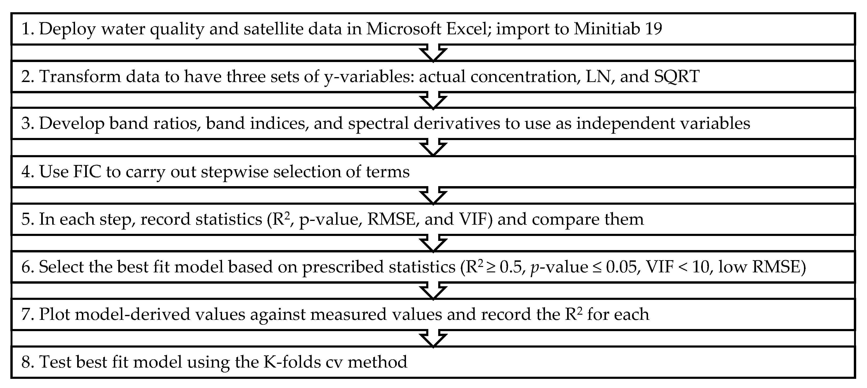
2.5. Best-Fit Model Selection and Validation

The first step in the model building was power transformation of the dependent water quality variables to increase the chances of improving the regression fits. Each of the three water quality parameters was transformed into its natural logarithm (LN) and square root (SQRT), and all three data types (actual values, LN, and SQRT) were used in the generation and selection of the best fit model.
This was followed by generating several independent variables through different methods of band combinations to increase the chances of developing strong regression models. The first set of independent variables included single bands, band ratios, and band indices. The band ratios were obtained by dividing two bands (e.g., ρRNIR−1). The band indices were the square of the normalized difference between surface reflectance values in two or more bands. These were paired with corresponding Chla, Turb, and SD (actual, LN, and SQRT) values for the development of regression models. The resulting statistics were recorded and evaluated.
In the following step, the independent variables were the surface reflectance values divided by their respective center wavelengths and 1st and 2nd derivatives of the surface reflectance spectra [11]. The first derivatives were designated dn with values ranging from d1 = (ρband-3 − ρband-2) ∗ (λband-3 − λband-2)−1 to dn−1 =band-(n+1) − ρband-n) ∗ (λband-(n+1) − λband-n)−1. The 2nd derivatives were designated d2n with values ranging from d21 = (d2 − d1) ∗ (λband-3 − λband-1)−1 to d2(n−1) = (dn+1 − dn) ∗ (λband-(n+2) − λband-n)−1. The value n is the band number, λ is the center wavelength, and ρ is the surface reflectance. These were combined with their corresponding water quality parameters for the development of regression models. Finally, we deployed all the independent variables generated above with their paired water quality parameters and ran them in the regression analysis.
The criteria considered in this study were the p-value, R2, Root Mean Square Error (RMSE), and Variance Inflation Factor (VIF). The regression terms that gave the best satisfaction of these criteria were selected for model building. The criteria were set as follows:
  • The relationships should be significant on a 95% confidence interval (α ≤ 0.05);
  • A strong relationship between the dependent variable and the predictors (R2 ≥ 0.5);
  • Low standard deviation of the residuals (RMSE) relative to the range of values;
  • Low correlation between the predictors (VIF < 10).
Selection of the best fit model was achieved using Minitab-19 statistical software [49]. The null hypothesis was that the surface reflectance from the bands, band combinations, and spectral derivatives did not predict variations in Chl-a, Turb, or SD, at a significance level (α) of 0.05. Each of the predictors was selected and evaluated using the Forward Information Criteria (FIC) in Minitab. The function is a stepwise selection that takes away and adds one variable at a time and determines selected statistics as it proceeds. This function is exhaustive and reshuffles variables until it determines that the best criteria are satisfied.
Model-derived values of each parameter were plotted against measured data that matched sampling periods and sites. At least 40 data points were randomly selected from the data and set aside for comparison to model derived values in scatter plots. The R2 was used to determine the extent to which the model-derived data agreed with the measured data.
Each best fit model was further tested using the K-folds cross-validation (cv) in Minitab. The advantage of the K-folds cv method over a single training/testing split is that every data point is used in both the training and testing sets. The data is divided into a certain number of partitions (K-folds) and each partition is used as a testing set while the rest of the data is used as a training set [50]. The average R2 and RMSE for 10 folds of cv were used to determine the validity of the models obtained. The procedure for the development of models, selection of the best fit model, and its validation are summarized in Figure 2.

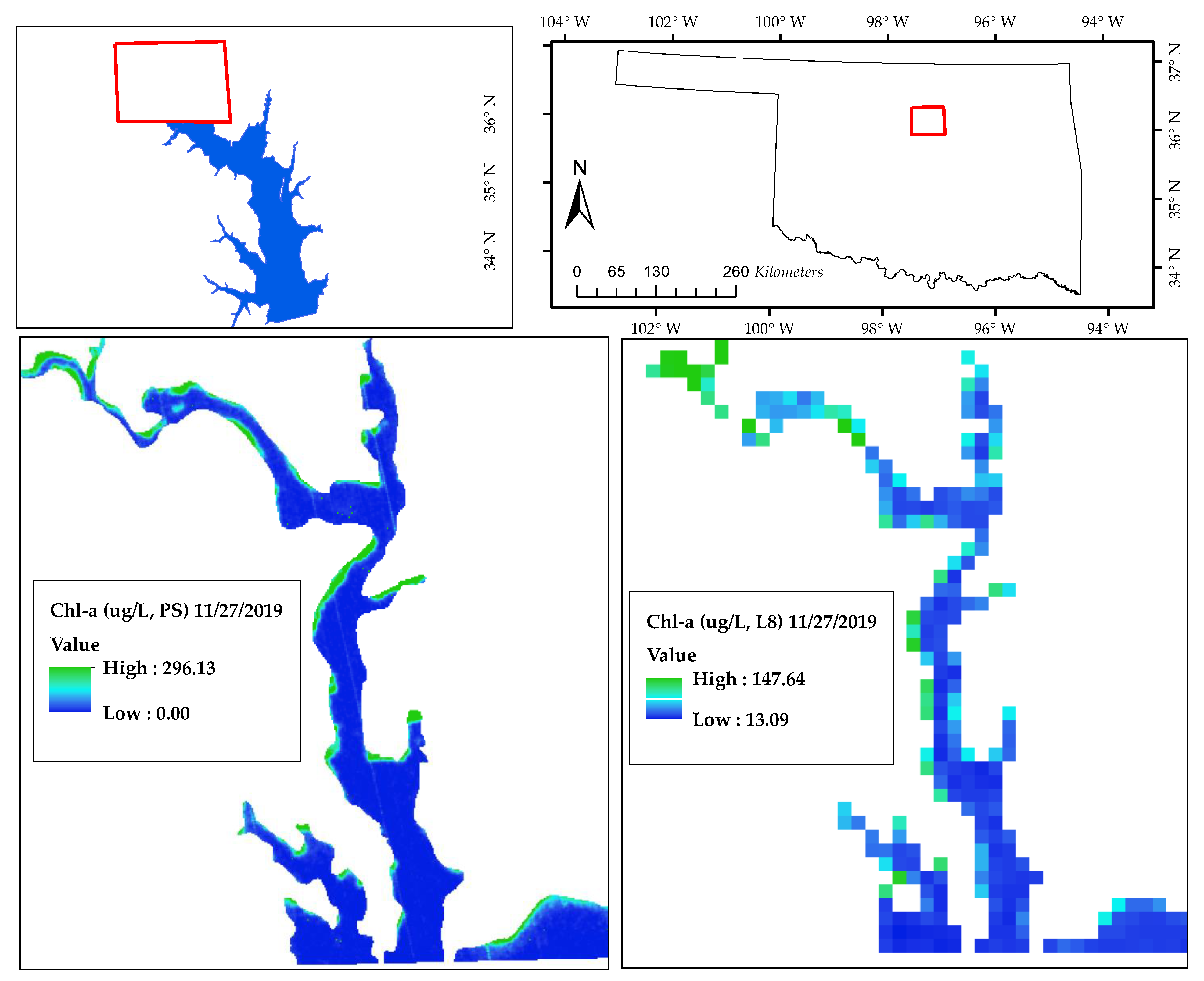
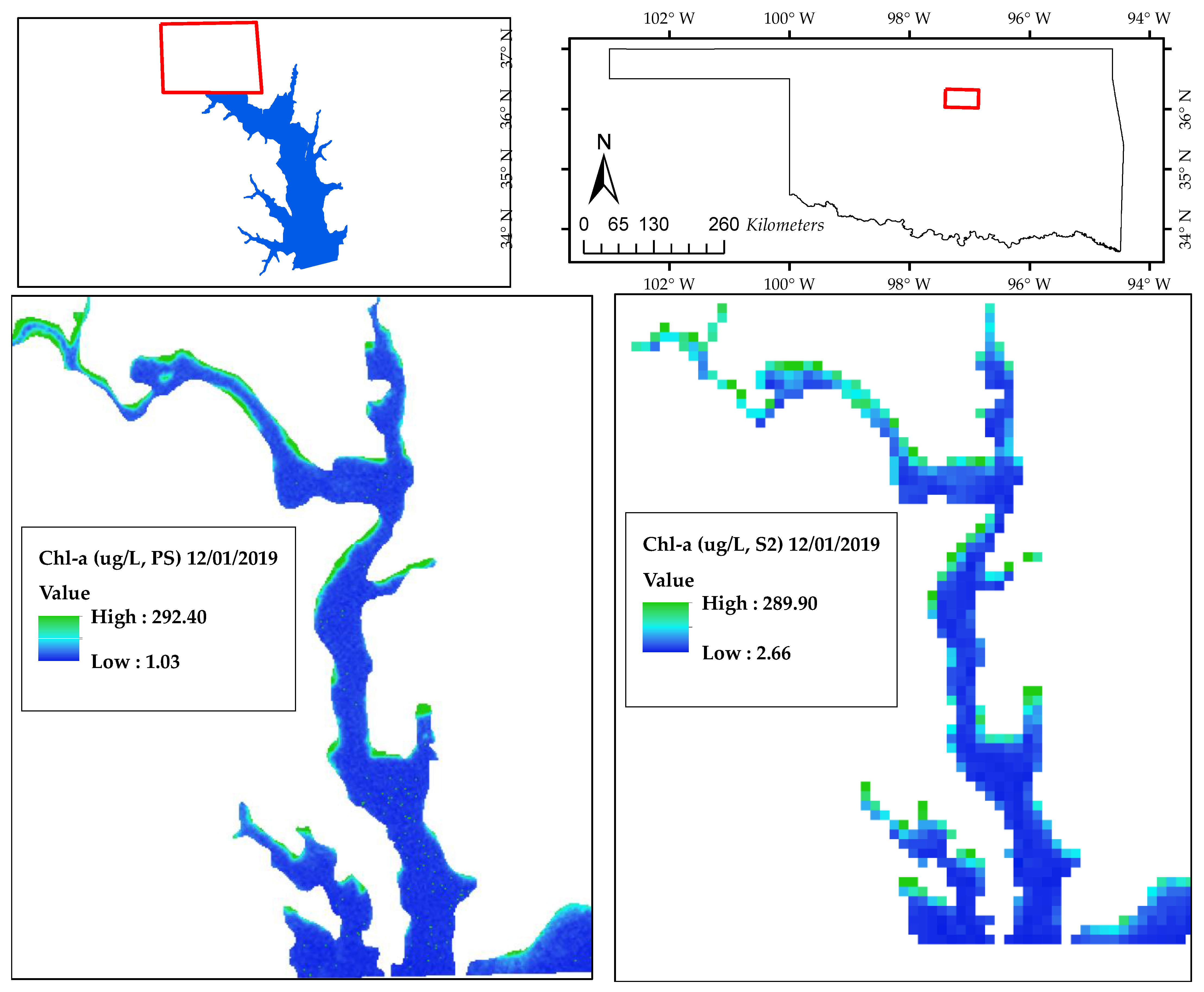
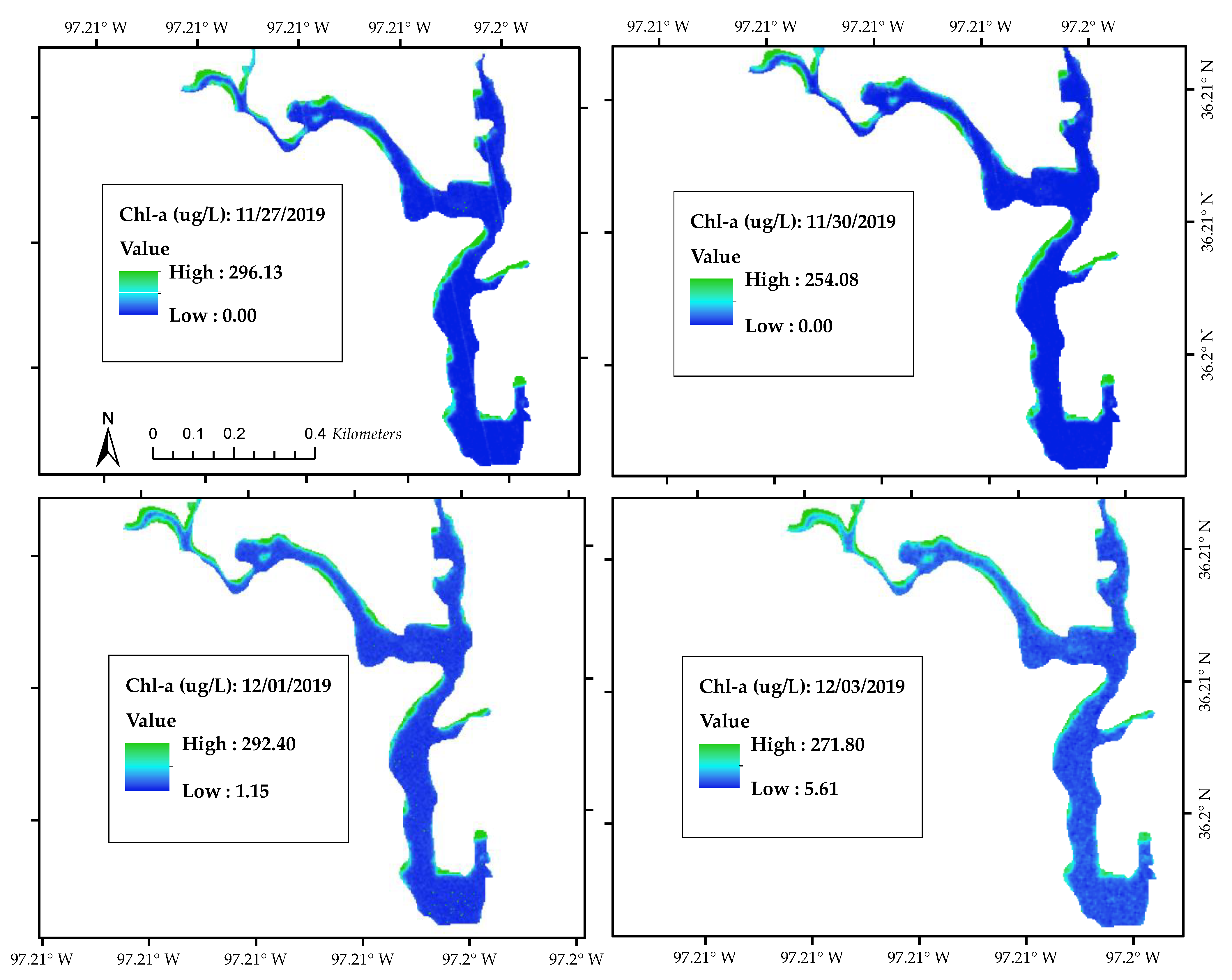
2.6. Case Study Application—Algal Bloom in Lake McMurtry, Oklahoma

We used an algal bloom event that occurred in Lake McMurtry, northcentral Oklahoma, from 27 November to 3 December 2019, to compare the spatial-temporal properties of the three satellites. PS had 4 cloud-free images (27 November, 30 November, 1 December, and 3 December 2019) available during this bloom event. In contrast, Landsat-8 had only one image with a cloud-free portion in the northern part of the lake (27 November 2019). Sentinel-2 also had only one image (1 December 2019) with a cloud-free portion that included the lake. These images were used to compare PS to Landsat-8 and Sentinel-2 in terms of their temporal and spatial resolutions. The Spatial Analyst tool of ArcMap 10.7.1 was used to compute pixel values of Chl-a in the areas of interest.

3. Results

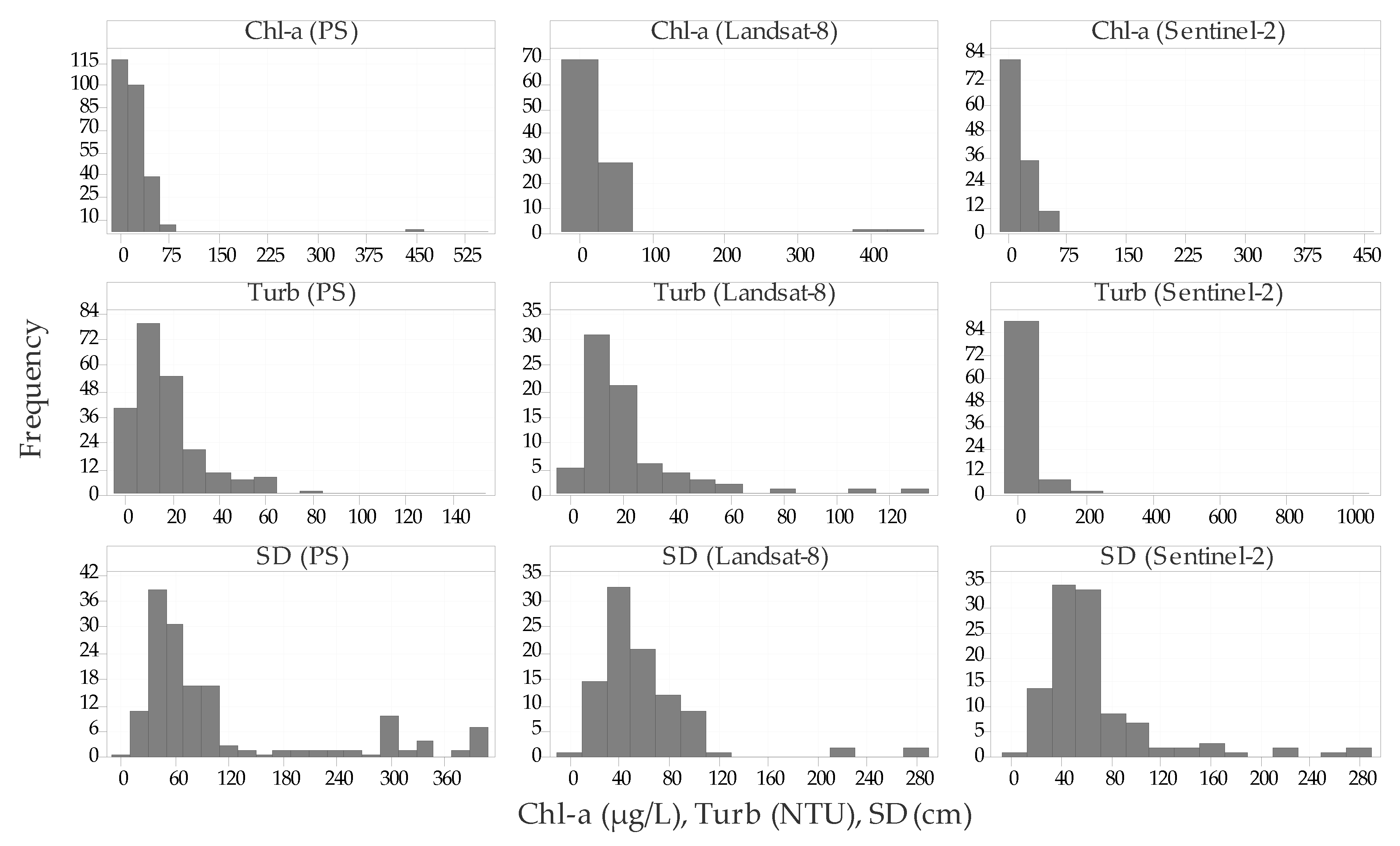
3.1. Range of Values of the Three Parameters

Chl-a concentrations in the study reservoirs ranged from 0.60 to 540 µg/L. Turb ranged from 0.00 to 966 NTU and SD ranged from 8.0 to 400 cm. PS had more data points to match with water quality than Landsat-8 and Sentinel-2 because of its daily flyover schedule. For PS, there were 207 data points for Chl-a, 225 data points for Turb, and 158 data points for SD. For Landsat-8, there were 100 data points for Chl-a, 75 data points for Turb, and 96 data points for SD. For Sentinel-2, there were 129 data points for Chl-a, 101 data points for Turb, and 113 data points for SD. Figure 3 shows the range of values of Chl-a, Turb, and SD.

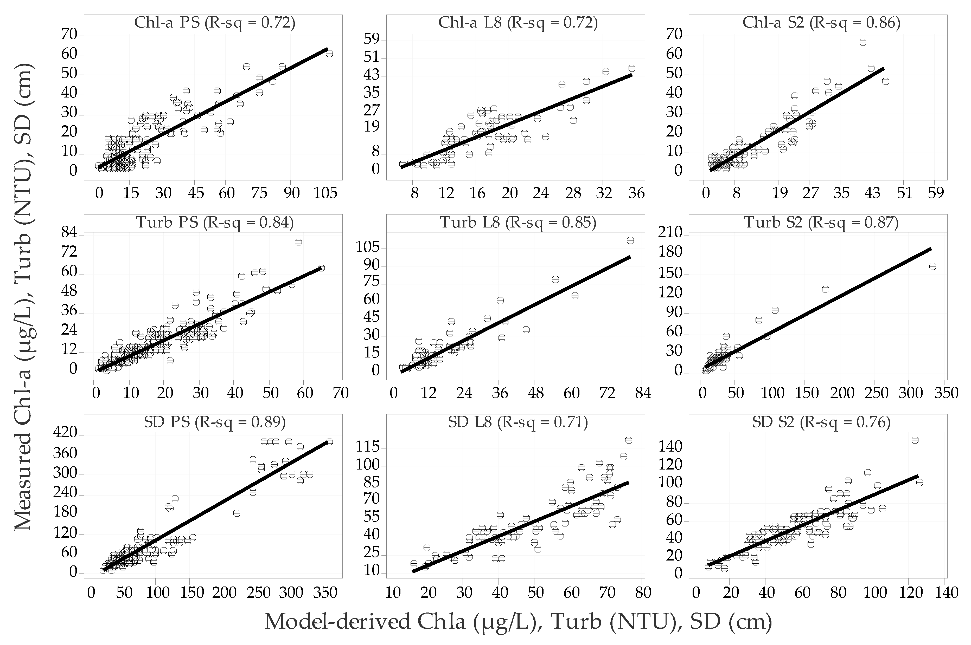
3.2. Best Fit Models

Equations (3)–(11) present the best fit regression equations for the three satellites.
PS based equations:
SQRT(Chl-a) = 1.24 − 89.10ρB + 79.10ρNIR + 9.67ρ((R+B−NIR)/(R+B+NIR))2 + 13.67ρ((G−NIR)/(G+NIR))2
LN(Turb) = 1.65 + 2.30ρ(R/G) − 0.035ρ(1/NIR) − 0.07ρ(1/R)
LN(SD) = 4.22 − 0.90ρ(R/B) + 0.02ρ(1/NIR) + 0.07 ρ(1/R)
where ρ is the surface reflectance value at a wavelength within the bands.
Landsat-8 based equations:
SQRT(Chl-a) = 4.778 − 45.5d4 − 123.03d5 − 26.33ρ(B/λB)
where d4 = (ρSWIR1 − ρNIR)/(λSWIR1 − λNIR), d5 = (ρSWIR2 − ρSWIR1)/(λSWIR2 − λSWIR1), λB, λSWIR1 and λSWIR2 are the center wavelength of the respective bands.
SQRT(Turb) = 4.67 + 9.86d2 + 41.70d24
where d2 = (ρR − ρG)/(λR − λG), and d24 = (d5 − d4)/( (λSWIR2 − λNIR).
LN(SD) = 4.1974 − 2.018d2 + 1.227d3 + 18.76d4 − 18.22d5
where d2 = (ρR − ρG)/(λR − λG), d3 = (ρNIR − ρR)/(λNIR − λR)
Sentinel-2 Based Equations:
SQRT(Chl-a) = 2.986 + 6.936d3 − 0.861d4 − 91.4d8
where d3 = (ρRE1 − ρR)/(λRE1 − λR), d4 = (ρRE2 − ρRE1)/(λRE2 − λRE1); and d8 = (ρSWIR2 − ρSWIR1)/(λSWIR2 − λSWIR1)
LN(Turb) = 0.076 − 29.80ρSWIR2 + 4.72ρ(R/B) − 3.38ρ((R−NIR)/(R+NIR))2
LN(SD) = 6.66 + 28.81ρSWIR2 − 15.34ρRE3 − 2.86ρ(R/G)
All the regression models for the three parameters provided significant relationships between the spectral data from each platform and their respective parameters. The p-values for the coefficients and constants were also significant (p < 0.01). Table 4 presents results of the statistical analysis for the overall regressions, coefficients, and constants in Equations (3)–(11).
The Chl-a R2 values for Sentinel-2 (R2 = 0.85) and Landsat-8 (R2 = 0.75) showed that the spectral data from these two satellites predict Chl-a better than PS (R2 = 0.58). Their Chl-a RMSE values were also lower than that for PS. These results imply that Landsat-8 and Sentinel-2 are preferable for detecting Chl-a reflectance over PS. The low VIF values (Maximum VIF < 10) in all three platforms indicate minimal collinearity between the regression terms. This was the case for all the parameters and all three satellites.
For Turb, PS and Sentinel-2 had comparable R2 values (0.79 and 0.78, respectively), while the R2 value for Landsat-8 was lower (R2 = 0.60). All the RMSE values were relatively low, indicating reliability in using all three platforms for sensing Turb in the study reservoirs. PS and Sentinel-2 are the preferred satellites for sensing Turb in the study reservoirs based on their R2 values.
For SD, the R2 in Sentinel-2 was the highest (R2 = 0.80) followed by PS (R2 = 0.76). The Landsat-8 value for SD was the lowest (R2 = 0.58). The RMSEs were low relative to the range of values in all three satellites. Based on these results, Sentinel-2 and PS are the preferred platforms for sensing SD in the study reservoirs.
Figure 4 presents scatter plots showing relationships between the values of Chl-a (µg/L), Turb (NTU), and SD (cm) predicted by the PS, Landsat-8 (L8), and Sentinel-2 (S2) spectra and those measured in the study reservoirs. The R2 (R-sq) values are displayed at the top of each graph along with the associated parameters and satellite platforms. The x-axis represents the model-derived values, and the y-axis represents the measured values. All three satellites showed strong relationships between measured and model-derived variables for the water quality parameters.

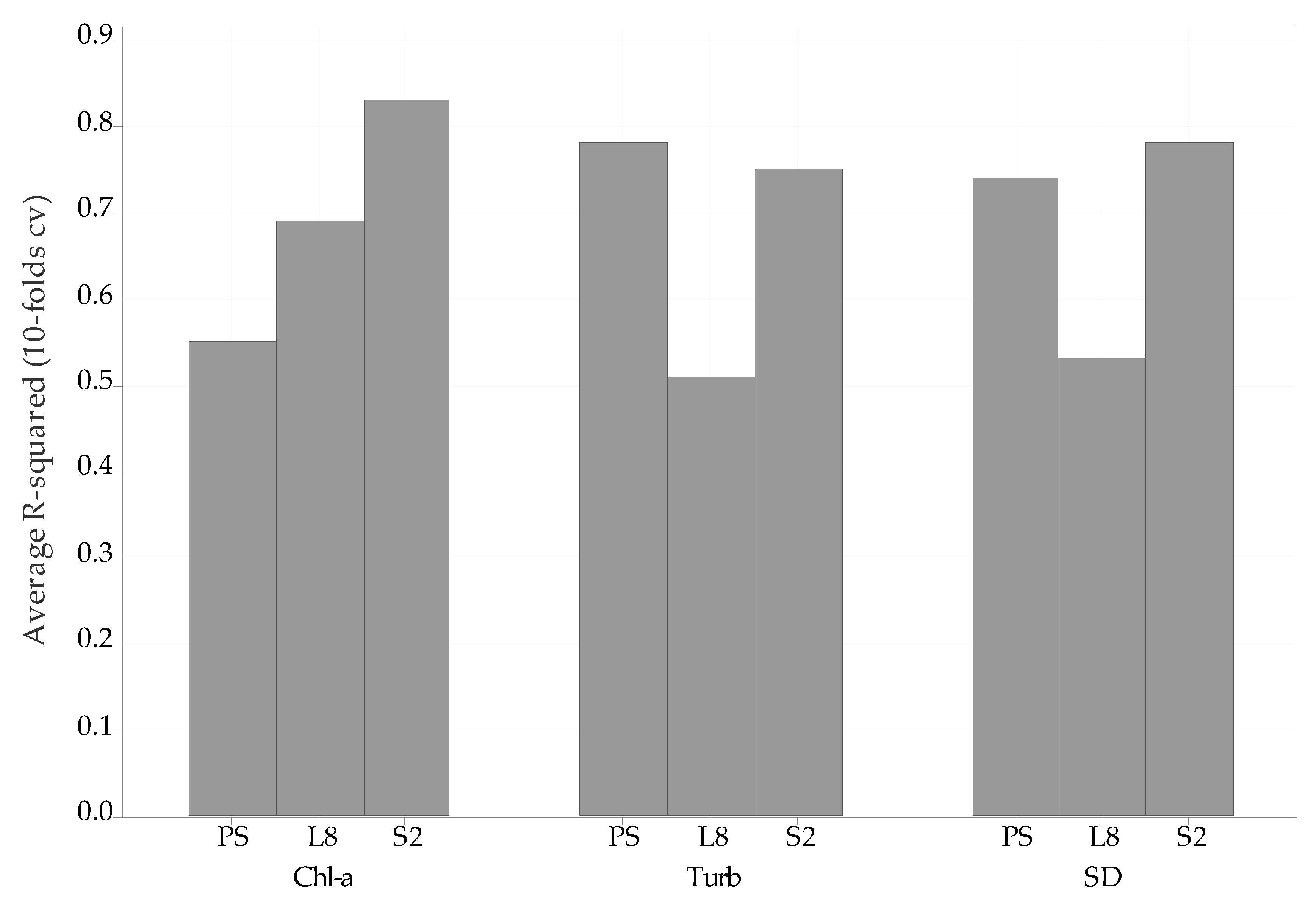
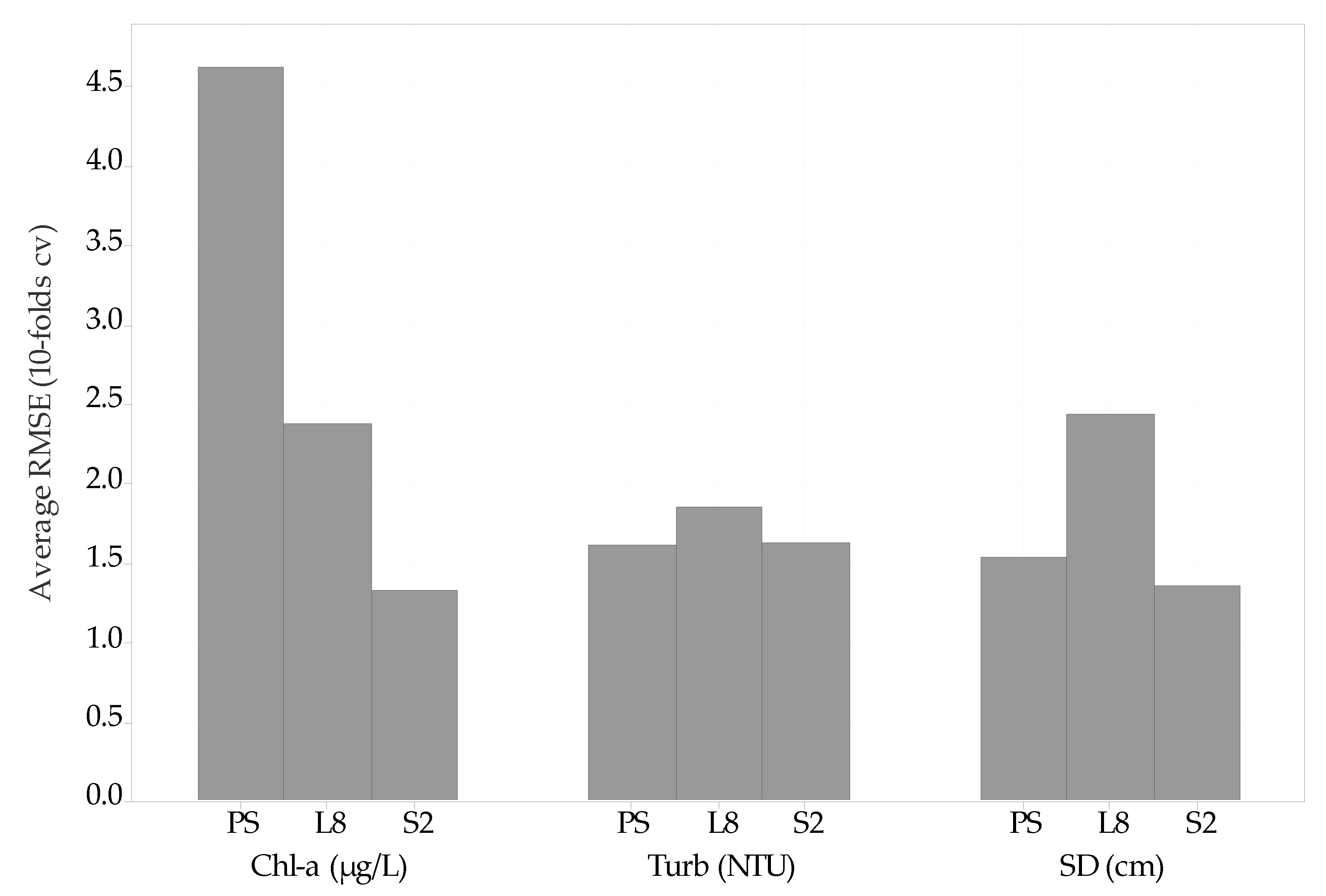
Validation of the Best Fit Models

Figure 5 shows the average R2 values obtained in the 10-fold cv of the parameters with PS, Landsat-8, and Sentinel-2. For Chl-a, Sentinel-2 had the highest average value (R2 = 0.83), followed by Landsat-8 (R2 = 0.69) and then PS (R2 = 0.55). PS had the highest average R2 for Turb (R2 = 0.78) followed by Sentinel-2 (R2 = 0.75), and Landsat-8 (R2 = 0.51). For SD, Sentinel-2 had the highest value (R2 = 0.78), followed by PS (R2 = 0.74), and Landsat-8 (R2 = 0.53).
Considering R2, the 10-folds cv showed that all three satellites are reliable for sensing all three parameters. Comparatively, Landsat-8 and Sentinel-2 were more reliable than PS for Chl-a sensing, while PS and Sentinel-2 were more reliable than Landsat-8 for Turb and SD sensing.
Figure 6 shows the average RMSE values obtained for the three parameters with the three satellites. The average RMSE values were below 5.0 for all three cases, which are considered low in reference to the range of values utilized in the study. The RMSE values for Turb and SD were comparable in the three satellites, while the PS RMSE for Chl-a (4.62 µg/L) was almost twice the amount in Landsat-8 (2.37 µg/L) and 3.5 times the Sentinel-2 amount (1.32 µg/L).
Similar to the observations made in the R2 validation results, the 10-folds cross validation showed that all three satellites are reliable for sensing all three parameters. The RMSEs also revealed that Landsat-8 and Sentinel-2 were more reliable than PS for Chl-a sensing, while PS and Sentinel-2 were more reliable than Landsat-8 for Turb and SD sensing.

3.3. Case Study Application—Algal Bloom in Lake McMurtry, Oklahoma

The onset of an algal bloom was reported in Lake McMurtry on 27 November 2019. The bloom grew and dissipated between 27 November and 5 December 2019. The Landsat-8 image that was available during these blooming dates (27 November) had a cloud-free portion in one of the areas where the bloom occurred. Sentinel-2 had only one available image with a cloud-free portion that included Lake McMurtry on December 1. There were four cloud-free PS images available during the blooming period. This event allowed for temporal and spatial comparisons in Chl-a mapping using models derived for PS, Landsat-8, and Sentinel-2. Figure 7 shows the PS and Landsat-8 maps for Chl-a on 27 November, 2019. Note that Chl-a concentrations were more visible in the littoral and riverine coves of the reservoir just as the bloom was observed when these sites were visited.
The PS-based Chl-a map showed the same pattern of Chl-a distribution as the Landsat-8 map. This shows that the models developed for both satellites estimate Chl-a similarly. The key difference in Figure 7 lies in the sizes of the pixels for PS (3 m) and Landsat-8 (30 m). The PS image gave a higher definition (finer spatial resolution) of Chl-a distribution in the focus area of the reservoir compared to Landsat-8. This observation is important for water quality sensing at the edges of the reservoir and in the riverine coves. The coarser spatial resolution of Landsat-8 could have caused the lower concentration range (13.09–147.64 µg/L) in those edges and coves compared to the PS range of values (0.00–296.13 µg/L). Figure 7 shows that the small pixel size from PS is better at detecting Chl-a near the lake’s edge and in the coves of the reservoir, which is where the bloom was most concentrated.
Figure 8 shows the PS and Sentinel-2 maps for Chl-a on 1 December 2019. We used this figure to compare Chl-a from PS imagery to that from Sentinel-2 imagery for this single date during an algal bloom. The PS-based Chl-a models gave the same pattern of Chl-a distribution in both PS and Sentinel-2 maps, demonstrating that both models estimated Chl-a similarly. The PS image gave a higher definition (finer spatial resolution) of Chl-a distribution in the focus area of the reservoir compared to Sentinel-2. Unlike Landsat-8, the Sentinel-2 model gave a similar concentration range as the PS model, probably owing to its higher spatial resolution (10 m). Figure 8 again shows that on 1 December 2019, the small pixel size from PS was better at defining the distribution of Chl-a (than Sentinel-2) near the lake’s edge and in the riverine coves of the reservoir, which was where the bloom was most concentrated.
Figure 9 presents PS Chl-a maps in the northwest cove of the reservoir. The images were acquired on dates between 27 November and 3 December. The algae had dispersed in the cove by 3 December. The bloom peaked and started dissipating just before this time, and no bloom was observed during ground-based observation on 5 December. Figure 9 shows several PS images from the same bloom from 27 November to 3 December, 2019. These images show the dynamic nature of the algal bloom as it changed daily. We also note that during this period of the bloom, there was only a single image available for both Landsat-8 and Sentinel-2. Of the 3 satellite platforms, PS was the only one with enough available/usable imagery to follow the dynamic nature of the algal bloom during this period.

4. Discussion

4.1. PlanetScope Nanosatellites

PlanetScope (PS) nanosatellites were originally developed for terrestrial and aquatic applications [51]. Our research contributes to a growing body of research [28] showing that PS is also applicable for use in water quality management applications. The accuracy of the models developed from PS spectra (based on R2 and RMSE values) for three key water quality parameters were relatively similar to those that have been developed for other water bodies using other satellites such as Landsat-8 and Sentinel-2 [22,25,44].
The independent variables of the Chl-a, Turb, and SD models for PS were the single bands, band ratios, and band indices. The spectral bands in the best fit PS model for Chl-a were B, NIR, ((R + B − NIR)/(R + B + NIR))2, and ((G − NIR)/(G + NIR))2. Chl-a reflects G and absorbs B and R during photosynthesis [15], which is probably why the B band has a negative linear relationship with Chl-a in the equation. We suggest that the square of the normalized difference between the visible bands (R + B) and the NIR band explains the impact of Turb on Chl-a reflectance, since both visible and NIR bands interact with both parameters [10,52]. The NIR band has also been used in previous satellite studies, especially at wavelengths close to the Red-Edge. NIR has been used mostly in combination with R [16]. Red may not be applicable in this case due to possible interference from Turb; agricultural runoff, shoreline erosion, and in-lake resuspension make Turb a primary source of reservoir impairment in the study area. The square of the normalized difference between G and NIR is not as common as that between R and NIR [10] at specific wavelengths. Our empirical results indicate that ((G − NIR)/(G + NIR))2 contributes significantly to Chl-a detection.
The independent variables that were selected for Turb were R/G, 1/NIR, and 1/R. The positive linear relationship between R/G and the natural log of Turb likely explains the ferric oxide-laden sediment load in the study area. The second and third terms had a negative linear relationship with Turb, and their effect may be minimal when the exponential function is considered. The opposite is the case for SD in which the inverse values of R and NIR gave positive linear relationships while the R/B gave a negative linear relationship with the parameter. Oklahoma’s Turb is mostly reddish in color, and it has an inverse relationship with SD [47]. Additionally, since water absorbs NIR, clear waters (high SD) would translate to low NIR reflectance. Similarly, R is associated with Turb and minimizes light penetration. The reverse order of independent variables for Turb and SD is consistent with past studies showing an inverse relationship between Turb and SD [53].

4.2. PlanetScope Compared to Landsat-8 and Sentinel-2

Although PS has finer spatial and temporal resolutions than Landsat-8 and Sentinel-2, the latter two satellites have more spectral bands. These additional bands contributed to better models for Chl-a in terms of the coefficient of determination (R2) and the error values. Those additional bands are not as susceptible to Turb as the NIR band [31]. Additionally, the spectral derivatives showed strong relationships with Chl-a in Landsat-8 and Sentinel-2. They also showed strong relationships with Turb and SD in Landsat-8.
In addition to the visible bands, the two SWIR bands in Landsat-8 and Sentinel-2 contributed significantly to Chl-a reflectance in the study reservoirs. This observation is consistent with the results obtained in previous studies. The SWIR band (λ = 1500–2500) appears to be less susceptible to scattering than the NIR band because of its longer wavelengths. This allows minimal Turb interference to this band compared to NIR [31]. The Red-Edge band in Sentinel-2 has been shown to better detect Chl-a than Landsat-8 bands [32] because it is not as susceptible to absorption or scattering. Wavelengths in this region have a strong linear relationship with Chl-a reflectance [54].
The PS and Sentinel-2 models outperformed Landsat-8 for Turb and SD, probably owing to their finer pixel sizes (3 and 10 m, respectively). Even though Sentinel-2 has a coarser spatial resolution than PS, our study suggests that the 10 m pixel is fine enough for detecting Turb in the study reservoirs. The agricultural practices, along with streambank and shoreline erosion, and in-lake resuspension of sediment in the study area are common sources of continuous sediment transport, which elevates Turb levels in waters in the region. The same explanation applies to SD since its values trend inversely with Turb.
PS is a commercial satellite whereas Landsat-8 and Sentinel-2 images are open source. Therefore, it may not be economically feasible to use PS to remotely sense water quality for all water resource applications. The bloom event from Lake McMurtry highlights a scenario where the finer spatial and temporal resolutions of PS can be used to remotely sense Chl-a. The algal bloom developed over several days in the reservoir (Figure 9). During this period, there were several cloud-free PS images compared to only one for Landsat-8 and Sentinel-2 images during the blooming event. These return periods of PS allowed for the detection and monitoring of bloom dynamics that changed daily and could not be measured from the other satellite platforms. This temporal advantage of PS provides an opportunity for lake managers to make informed decisions regarding response efforts such as the duration of beach closures during HABs.
The finer spatial resolution of PS may allow for the remote sensing of water quality in smaller ponds and reservoirs compared to coarser-resolution satellites. Small (farm) ponds are important in agricultural watersheds and they often experience high nutrient and sediment loads. Oklahoma has thousands of ponds ranging in size between 0.001 km2 and 0.04 km2. Because of their small size, they are difficult to monitor with ground-based sampling or with Landsat-8 or Sentinel-2. For example, a 0.001-km2 pond would be covered with only one Landsat-8 pixel or 10 Sentinel-2 pixels (considering Sentinel-2 data with 10-m pixel size). For the same 0.001-km2 pond, a PS image would have approximately 111 pixels. As such, PS data with finer spatial resolution (3 m) could be used to assess more pixels in the ponds and better detect small-scale changes in water quality.
This study covered 13 reservoirs located in predominately agriculturally dominated watersheds that are dominated by agricultural practices. Additional studies are needed to determine if our models developed for agricultural landscapes could be used in other reservoirs in the region and around the world. Additional studies are also required to test and refine our models in areas with dominant human activities other than agriculture.
A limitation to using PS imagery is that it has fewer spectral bands compared to Landsat-8 and Sentinel-2. PS also has many satellites each providing image tiles with properties that may vary from each other. This may require normalization of those image tiles, which was beyond the scope of this study. We selected image tiles with the same satellite ID to minimize the likelihood of this source of error. However, a future application of PS imagery for water quality monitoring requires normalization of multiple image tiles to ensure comparability. Such image analysis, in addition to acquiring the imagery, makes it costly for PS use for water quality monitoring at a regional scale. Furthermore, the scalability of PS imagery for cost recovery in water quality monitoring is limited to areas with high frequency of cloud-free days. A key benefit of PS data is using its finer spatial and temporal resolutions to measure dynamic water quality parameters in small reservoirs and coves of larger reservoirs that are not feasible to monitor with moderate-coarser resolution satellites and are inaccessible for ground-based monitoring.

5. Conclusions

Traditional water quality monitoring is limited to specific sample locations and infrequent sample visits. These limitations create spatial and temporal gaps during which water quality impairment may occur and pose exposure risks. This study explored the utility of satellites to detect water quality in those spatial and temporal gaps in agricultural watersheds. We compared the spatial, temporal, and spectral resolutions of PS to those of Landsat-8 and Sentinel-2 for sensing three water quality parameters in Oklahoma reservoirs. We used three years (2017–2020) of surface reflectance spectra for PS, Landsat-8, and Sentinel-2 to develop empirical models for Chl-a, Turb, and SD in 13 reservoirs in Oklahoma. Multiple linear regression models were developed using surface reflectance from the bands, band ratios, and band indices of these water quality parameters.
Overall, the spectral data from each of the three satellite platforms (PS, Landsat-8, and Sentinel-2) had significant relationships with Chl-a, Turb, and SD. We conclude that the finer spatial and temporal resolutions in PS give it the capabilities that are comparable to Landsat-8 and Sentinel-2 for sensing key water quality parameters in the study reservoirs. However, this capability is moderated by the fewer spectral bands and the cost to acquire the PS imagery given that Landsat-8 and Sentinel-2 data are free. We identified scenarios where it may be more beneficial to use PS compared to Landsat-8 and Sentinel-2. PS is better suited for measuring water quality variables that vary daily, in small ponds and reservoirs where satellites with coarser spatial resolution do not provide enough pixels and at the edge of water bodies where variation in water quality requires fine-scale detection.
Future research should work to combine PS, Landsat-8, and Sentinel-2 to develop a predictive monitoring tool that utilizes their tradeoffs to increase our ability to understand water quality dynamics. Key areas of a combined satellite approach [55,56,57,58] could include targeted monitoring of hot spot areas, frequent monitoring of phytoplankton and sediments from nutrient-rich runoff, wider spatial and temporal coverage than ground-based monitoring programs can accomplish, and ultimately, effective use of resources for water quality monitoring.

Author Contributions

Conceptualization: all authors; methodology: A.S.M.; software: A.S.M. and M.E.M.; validation: A.S.M., H.G., A.R.D. and M.E.M.; formal analysis: all authors; investigation: A.S.M.; resources: K.L.W., S.H.S. and A.R.D.; data curation: A.S.M.; writing—original draft preparation: A.S.M.; writing—review and editing: all authors; supervision: K.L.W., S.H.S. and A.R.D.; project administration: K.L.W., S.H.S. and A.R.D.; funding acquisition: K.L.W., S.H.S. and A.R.D. All authors have read and agreed to the published version of the manuscript.

Funding

This research received no external funding.

Acknowledgments

The Grand River Dam Authority and the Water Quality Division of the Oklahoma Water Resources Board provided the data for this study. The Lake McMurtry Friends provided support for algal bloom observation from 27 November to 5 December 2019.

Conflicts of Interest

The authors declared no conflict of interest.

References

  1. Henley, W.F.; Patterson, M.A.; Neves, R.J.; Lemly, A.D. Effects of Sedimentation and Turbidity on Lotic Food Webs: A Concise Review for Natural Resource Managers. Rev. Fish. Sci. 2010, 8, 125–139. [Google Scholar] [CrossRef] [Green Version]
  2. Havens, K.E.; James, R.T.; East, T.L.; Smith, V.H. N:P ratios, light limitation, and cyanobacterial dominance in a subtropical lake impacted by non-point source nutrient pollution. Env. Pol. 2003, 122, 379–390. [Google Scholar] [CrossRef]
  3. Chen, M.; Ding, S.; Chen, X.; Sun, Q.; Fan, X.; Lin, J.; Ren, M.; Yang, L.; Zhang, C. Mechanisms driving phosphorus release during algal blooms based on hourly changes in iron and phosphorus concentrations in sediments. Water Res. 2018, 133, 153–164. [Google Scholar] [CrossRef]
  4. Larsen, D.P.; Urquhart, N.S.; Kugle, D.L. Regional Scale Monitoring of Indicators of Trophic Conditions of Lakes. JAWRA 1995, 31, 117–140. [Google Scholar] [CrossRef]
  5. Urquhart, N.S.; Paulsen, S.G.; Larsen, D.P. Monitoring for policy-relevant regional trends over time. Ecol. Appl. 1998. [Google Scholar] [CrossRef]
  6. Rodríguez, J.P.; Beard, T.D., Jr.; Bennett, E.M.; Cumming, G.S.; Cork, S.J.; Agard, J.; Dobson, A.P.; Peterson, G.D. Trade-offs across space, time, and ecosystem services. Ecol. Soc. 2006, 11. [Google Scholar] [CrossRef] [Green Version]
  7. Harvey, E.T.; Kratzer, S.; Philipson, P. Satellite-based water quality monitoring for improved spatial and temporal retrieval of chlorophyll-a in coastal waters. Remote Sens. Environ. 2015, 158, 417–430. [Google Scholar] [CrossRef]
  8. Olmanson, L.; Brezonik, P.; Bauer, M. Remote Sensing for Regional Lake Water Quality Assessment: Capabilities and Limitations of Current and Upcoming Satellite Systems. In The Handbook of Environmental Chemistry; Springer: Cham, Switzerland, 2015; Volume 33, pp. 111–140. [Google Scholar]
  9. Han, L.; Rundquist, D.C. Comparison of NIR/RED ratio and first derivative of reflectance in estimating algal-chlorophyll concentration: A case study in a turbid reservoir. Remote Sens. Environ. 1997, 62, 253–261. [Google Scholar] [CrossRef]
  10. Mishra, S.; Mishra, D.R. Normalized difference chlorophyll index: A novel model for remote estimation of chlorophyll-a concentration in turbid productive waters. Remote Sens. Environ. 2012, 117, 394–406. [Google Scholar] [CrossRef]
  11. Becker, B.L.; Lusch, D.P.; Qi, J. Identifying optimal spectral bands from in situ measurements of Great Lakes coastal wetlands using second-derivative analysis. Remote Sens. Environ. 2005, 97, 238–248. [Google Scholar] [CrossRef]
  12. Liu, L.; Lee, S.; Chahl, J.S. Transformation of a high-dimensional color space for material classification. J. Opt. Soc. Am. A 2017, 34, 523–532. [Google Scholar] [CrossRef] [PubMed]
  13. Mhosisi, M.; Dube, T.; Nhiwatiwa, T.; Choruma, D. Testing utility of Landsat 8 for remote assessment of water quality in two subtropical African reservoirs with contrasting trophic states. Geocarto Int. 2017, 33, 667–680. [Google Scholar]
  14. USEPA. World Health Organization (WHO) 1999 Guideline Values for Cyanobacteria in Freshwater. 2003. Available online: https://www.epa.gov/cyanohabs/world-health-organization-who-1999-guideline-values-cyanobacteria-freshwater (accessed on 13 January 2021).
  15. Jensen, J.R. Introductory Digital Image Processing—A Remote Sensing Perspective, 4th ed.; Botting, C., Ed.; Pearson Education Inc.: Columbia, SC, USA, 2015. [Google Scholar]
  16. Moses, W.J.; Gitelson, A.A.; Berdnikov, S.; Povazhnyy, V. Satellite Estimation of Chlorophyll-a Concentration Using the Red and NIR Bands of MERIS—The Azov Sea Case Study. IEEE Geosci. Remote Sens. Lett. 2009, 6, 845–849. [Google Scholar] [CrossRef]
  17. Tebbs, E.J.; Harper, D.M.; Remedios, J.J. Remote sensing of chlorophyll-a as a measure of cyanobacterial biomass in Lake Bogoria, a hypertrophic, saline–alkaline, flamingo lake, using Landsat ETM+. Remote Sens. Environ. 2013, 135, 92–106. [Google Scholar] [CrossRef]
  18. Yacobi, Y.Z.; Moses, W.J.; Kaganovsky, S.; Sulimani, B.; Leavitt, B.C.; Gitelson, A.A. NIR-red reflectance-based algorithms for chlorophyll-a estimation in mesotrophic inland and coastal waters: Lake Kinneret case study. Water Res. 2011, 45, 2428–2436. [Google Scholar] [CrossRef] [Green Version]
  19. Torbick, N.; Hu, F.; Zhang, J.; Qi, J.; Zhang, H.; Becker, B. Mapping Chlorophyll-a Concentrations in West Lake, China using Landsat 7 ETM+. Great Lakes Res. 2008, 34, 559–565. [Google Scholar] [CrossRef]
  20. Torbick, N.; Hessionb, S.; Hagena, S.; Wiangwangb, N.; Beckerc, B.; Qib, J. Mapping inland lake water quality across the Lower Peninsula of Michigan using Landsat TM imagery. Int. J. Remote Sens. 2013, 34, 7607–7624. [Google Scholar] [CrossRef]
  21. Rotta, L.H.S.; Alcântara, E.H.; Watanabe, F.S.Y.; Rodrigues, T.W.P.; Imai, N.N. Atmospheric correction assessment of SPOT-6 image and its influence on models to estimate water column transparency in tropical reservoir. Remote Sens. Appl. Soc. Environ. 2016, 4, 158–166. [Google Scholar] [CrossRef]
  22. Allee, R.J.; Johnson, J.E. Use of satellite imagery to estimate surface chlorophyll-a and Secchi disc depth of Bull Shoals Reservoir, Arkansas, USA. Int. J. Remote Sens. 1999, 20, 1057–1072. [Google Scholar] [CrossRef]
  23. Olmanson, L.G.; Brezonik, P.L.; Finlay, J.C.; Bauer, M.E. Comparison of Landsat 8 and Landsat 7 for regional measurements of CDOM and water clarity in lakes. Remote Sens. Environ. 2016. [Google Scholar] [CrossRef]
  24. Nguyen, U.N.T.; Pham, L.T.H.; Dang, T.D. An automatic water detection approach using Landsat 8 OLI and Google Earth Engine cloud computing to map lakes and reservoirs in New Zealand. Environ. Monit. Assess. 2019, 191. [Google Scholar] [CrossRef] [PubMed]
  25. Ansper, A.; Alikas, K. Retrieval of Chlorophyll a from Sentinel-2 MSI Data for the European Union Water Framework Directive Reporting Purposes. Remote Sens. 2019, 11, 64. [Google Scholar] [CrossRef] [Green Version]
  26. ESA. Sentinel-2. European Space Agency, 2020. Available online: https://sentinel.esa.int/web/sentinel/missions/sentinel-2 (accessed on 14 January 2021).
  27. Poursanidis, D.; Traganos, D.; Chrysoulakis, N.; Reinartz, P. Cubesats Allow High Spatiotemporal Estimates of Satellite-Derived Bathymetry. Remote Sens. 2019, 11, 1299. [Google Scholar] [CrossRef] [Green Version]
  28. Milad, N.-J.; Bovolo, F.; Bruzzone, L.; Gege, P. Physics-based Bathymetry and Water Quality Retrieval Using PlanetScope Imagery: Impacts of 2020 COVID-19 Lockdown and 2019 Extreme Flood in the Venice Lagoon. Remote Sens. 2020, 12, 2381–2398. [Google Scholar]
  29. Pramaditya, W.; Wahyu, L. Assessment of PlanetScope images for benthic habitat and seagrass species mapping in a complex optically shallow water environment. Int. J. Remote Sens. 2018, 39, 5739–5765. [Google Scholar]
  30. Gabr, B.; Ahmed, M.; Marmoush, Y. PlanetScope and Landsat 8 Imageries for Bathymetry Mapping. J. Mar. Sci. Eng. 2020, 8, 143. [Google Scholar] [CrossRef] [Green Version]
  31. Kuhn, C.; de Matos Valerio, A.; Ward, N.; Loken, L.; Sawakuchi, H.O.; Kampel, M.; Richey, J.; Stadler, P.; Crawford, J.; Striegl, R.; et al. Performance of Landsat-8 and Sentinel-2 surface reflectance products for river remote sensing retrievals of chlorophyll-a and turbidity. Remote Sens. Environ. 2019, 224, 104–118. [Google Scholar] [CrossRef] [Green Version]
  32. Bramich, J.; Bolch, C.J.S.; Fischer, A. Improved red-edge chlorophyll-a detection for Sentinel 2. Ecol. Indic. 2021, 120, 106876–106885. [Google Scholar] [CrossRef]
  33. OWRB. Water Facts. 14 March 2018. Available online: https://www.owrb.ok.gov/util/waterfact.php (accessed on 13 February 2021).
  34. OWRB. Data & Maps—Surface Water. Oklahoma Water Resources Board, 2020. Available online: http://www.owrb.ok.gov/maps/PMG/owrbdata_SW.html (accessed on 12 February 2021).
  35. Williams, K.W. Farm Ponds. In The Encyclopedia of Oklahoma History and Culture; Oklahoma Historical Society: Oklahoma City, OK, USA, 2007. [Google Scholar]
  36. Arango, J.G.; Holzbauer-Schweit, B.K.; Nairn, R.W.; Knox, R.C. Generation of geolocated and radiometrically corrected true reflectance surfaces in the visible portion of the electromagnetic spectrum over large bodies of water using images from a sUAS. J. Unmanned Veh. Syst. 2020, 8, 172–185. [Google Scholar] [CrossRef]
  37. OWRB. Lakes, Oklahoma Water Resources Board. 21 July 2020. Available online: https://www.owrb.ok.gov/quality/monitoring/bumplakes.php (accessed on 12 February 2021).
  38. OWRB. Oklahoma Lakes Report—Benificial Use Monitoring Program; Oklahoma Water Resource Board (OWRB): Oklahoma City, OK, USA, 2017.
  39. Kloiber, S.M.; Brezonik, P.L.; Olmanson, L.G.; Bauer, M.E. A procedure for regional lake water clarity assessment using Landsat multispectral data. Remote Sens. Environ. 2002, 82, 38–47. [Google Scholar] [CrossRef]
  40. OWRB. Standard Operating Procedure for the Collection and Processing of Chlorophyll-a Samplesin Lakes. November 2019. Available online: https://www.owrb.ok.gov/quality/monitoring/bump/pdf_bump/Lakes/SOPs/Chlorophyll-aCollectionSOP.pdf (accessed on 1 February 2021).
  41. OWRB. Standard Operating Procedure for the Measurement of Turbidity in Lakes; Oklahoma Water Resources Board: Oklahoma City, OK, USA, 2005.
  42. Planet. Planet Imagery Product Specifications. 2019. Available online: https://www.planet.com/products/planet-imagery/ (accessed on 10 February 2021).
  43. USGS. Earth Explorer. 17 May 2018. Available online: https://earthexplorer.usgs.gov/ (accessed on 15 January 2021).
  44. McCullough, M.; Loftin, C.S.; Sader, S.S. Combining lake and watershed characteristics with Landsat TM data for remote estimation of regional lake clarity. Remote Sens. Environ. 2012, 123, 109–115. [Google Scholar] [CrossRef]
  45. Kirk, T.O. Light and Photosynthesis in Aquatic Ecosystems, 3rd ed.; Cambridge University Press: New York, NY, USA, 2011. [Google Scholar]
  46. Salem, S.I.; Higa, H.; Kim, H.; Kobayashi, H.; Oki, K.; Oki, T. Assessment of Chlorophyll-a Algorithms Considering Different Trophic Statuses and Optimal Bands. Sensors 2017, 17, 1746. [Google Scholar] [CrossRef] [PubMed] [Green Version]
  47. Scott, D.; Apblett, A.; Materer, N.F. Iron-rich Oklahoma Clays as a Natural Source of Chromium in Monitoring Wells. J. Environ. Monit. 2011, 13, 3380–3385. [Google Scholar] [CrossRef] [PubMed]
  48. Oyama, Y.; Matsushita, B.; Fukushima, T. Distinguishing surface cyanobacterial blooms and aquatic macrophytes using Landsat/TM and ETM+ shortwave infrared bands. Remote Sens. Environ. 2015, 157, 35–47. [Google Scholar] [CrossRef]
  49. Minitab. Minitab 19. 2021. Available online: https://www.minitab.com/en-us/ (accessed on 2 February 2021).
  50. Bengio, Y.; Grandvalet, Y. No Unbiased Estimator of the Variance of K-Fold Cross-Validation. J. Mach. Learn. Res. 2004, 5, 1089–1105. [Google Scholar]
  51. Nagel, G.W.; de Moraes Novo, E.M.L.; Kampel, M. Nanosatellites applied to optical Earth observation: A review. Ambiente Água Interdiscip. J. Appl. Sci. 2020. [Google Scholar] [CrossRef]
  52. Robert, E.; Grippa, M.; Kergoat, L.; Pinet, S.; Gal, L.; Cochonneau, G.; Martinez, J.-M. Monitoring water turbidity and surface suspended sediment concentration of the Bagre Reservoir (Burkina Faso) using MODIS and field reflectance data. Int. J. Appl. Earth Obs. Geoinf. 2016, 52, 243–251. [Google Scholar] [CrossRef]
  53. Rounds, S. Estimation of Secchi Depth from Turbidity Data in the Willamette River at Portland, OR (14211720). Oregon Water Science Center, 2016. Available online: https://or.water.usgs.gov/will_morrison/secchi_depth_model.html (accessed on 2 March 2021).
  54. Gitelson, A.; Gurlin, D.; Moses, W.J.; Barrow, T. A bio-optical algorithm for the remote estimation of the chlorophyll-a concentration in case 2 waters. Environ. Res. Lett. 2009, 4. [Google Scholar] [CrossRef]
  55. Claverie, M.; Ju, J.; Masek, J.G.; Dungan, J.L.; Vermote, E.F.; Roger, J.-C.; Skakun, S.V.; Justice, C. The Harmonized Landsat and Sentinel-2 surface reflectance data set. Remote Sens. Environ. 2018, 2019, 145–161. [Google Scholar] [CrossRef]
  56. Houborg, R.; McCabe, M.F. Daily Retrieval of NDVI and LAI at 3 m Resolution via the Fusion of CubeSat, Landsat, and MODIS Data. Remote Sens. 2018, 10, 890. [Google Scholar] [CrossRef] [Green Version]
  57. Houborg, R.; McCabe, M.F. A Cubesat enabled Spatio-Temporal Enhancement Method (CESTEM) utilizing Planet, Landsat and MODIS data. Remote Sens. Environ. 2018, 209, 211–226. [Google Scholar] [CrossRef]
  58. Yan, L.; Roy, D.P.; Zhang, H.; Li, J.; Huang, H. An Automated Approach for Sub-Pixel Registration of Landsat-8 Operational Land Imager (OLI) and Sentinel-2 Multi Spectral Instrument (MSI) Imagery. Remote Sens. 2016, 8, 520. [Google Scholar] [CrossRef] [Green Version]
Figure 1. Map of Oklahoma showing the BUMP reservoirs across the state (grey polygons and speckles) and the 13 reservoirs used in this study (in colors). The spatial data for this map were obtained from the Oklahoma Water Resource Board’s website [34].
Remotesensing 13 01847 g001
Figure 2. Flow diagram showing the procedure for model development, model selection, and model validation.
Remotesensing 13 01847 g002
Figure 3. Histograms of the Chl-a (µg/L), Turb (NTU), and SD (cm) data from the study reservoirs that correspond to their respective PS, Landsat-8, and Sentinel-2 images.
Remotesensing 13 01847 g003
Figure 4. Scatter plots showing relationships between the model-derived concentrations and measured concentrations of Chl-a (µg/L), Turb (NTU), and SD (cm) with PS, Landsat-8 (L8), and Sentinel-2 (S2). The R2 (R-sq) values are displayed at the top of each graph along with the associated parameters and satellite platforms.
Remotesensing 13 01847 g004
Figure 5. Average R2 values in the 10-fold cv of the parameters with PS, Landsat-8, and Sentinel-2.
Remotesensing 13 01847 g005
Figure 6. Average RMSE values in the 10-fold cv of the parameters with PS, Landsat-8, and Sentinel-2.
Remotesensing 13 01847 g006
Figure 7. PS (Left) and Landsat-8 (Right) maps of Chl-a in Lake McMurtry, northcentral Oklahoma. Both satellites acquired their images on 27 November 2019, during an active algal bloom event. The overview maps at the top show the location of Lake McMurtry in Oklahoma (Top Right spec in a red box) and Lake McMurtry (Top Left) showing the focus area delineated in a red box. The color bars represent concentration ranges as estimated by each of the two satellites.
Remotesensing 13 01847 g007
Figure 8. PS (Left) and Sentinel-2 (Right) maps of Chl-a in Lake McMurtry, northcentral Oklahoma. Both satellites acquired their images on 1 December 2019, during an active algal bloom event. The overview maps at the top show the location of Lake McMurtry in Oklahoma (Top right spec in a red box) and Lake McMurtry (Top left) showing the focus area delineated by a red box. The color bars represent concentration ranges as estimated by each of the two satellites.
Remotesensing 13 01847 g008
Figure 9. PlanetScope maps of Chl-a on four dates of image acquisition in Lake McMurtry, northcentral Oklahoma. The upper left panel is from an image acquired on 27 November 2019; the upper right panel is from an image acquired on 30 November 2019; the lower left panel is from an image acquired on 1 December 2019; the bottom right panel is from an image acquired on 3 December 2019. The color bars in the legends represent Chl-a concentration ranges on each date.
Remotesensing 13 01847 g009
Table 1. Characteristics of Landsat-8, Sentinel-2, and PS.
CharacteristicsPSLandsat-8Sentinel-2
Revisit time (temporal resolution)Daily16 days10 days with each satellite (Sentinel 2A and 2B). Five days with combined satellites.
Spectral resolutionFour 3-m bandsEight 30-m bands, two 100-m bands, one 15-m panchromatic band (11 bands)Four 10-m bands, six 20-m bands, and three 60-m bands (13 bands)
Pixel size (spatial resolution)More pixels in small areas/reservoirsFew or no pixels in small areas/reservoirs (e.g., with area 0.001 km2 or less)Few pixels in small areas/reservoirs (e.g., with area 0.001 km2 or less)
Bandwidth in nm (visible and NIR)Blue: 465–517; Green: 547–595; Red: 650–682; NIR: 846–888Blue: 435–512; Green: 533–590; Red: 636–673; NIR: 851–879, Shortwave IR1 (SWIR1): 1570–1650; Shortwave IR2 (SWIR2): 2110–2290Blue: 458–523; Green: 543–578; Red: 650–680; Red-Edge (RE1): 698–713; Red-Edge (RE2): 733–748; Red-Edge (RE3): 773–793; NIR: 785–899; SWIR1: 1565–1655; SWIR2: 2100–2280
Availability of free imagery10,000 km2 per month for education purposeUnlimitedUnlimited
Table 2. Characteristics of the reservoirs used in this study. This information was obtained from the Oklahoma Water Resource Board’s website [37].
ReservoirSurface Area (km2)Trophic StatusImpairment Status
Chl-aTurb
Arcadia7.40HypereutrophicImpairedImpaired
Broken Bow57.50MesotrophicNot impairedNot impaired
Canton32.00HypereutrophicInsufficient dataImpaired
Eucha11.60EutrophicImpairedNot impaired
Fort Gibson60.30EutrophicInsufficient dataNot impaired
Foss35.61MesotrophicInsufficient dataImpaired
Hefner10.11HypereutrophicInsufficient dataNot impaired
Grand188.20EutrophicInsufficient dataNot impaired
Kaw68.96HypereutrophicInsufficient dataImpaired
McMurtry4.67EutrophicInsufficient dataImpaired
Oologah119.22MesotrophicInsufficient dataImpaired
Thunderbird24.60HypereutrophicImpairedImpaired
Waurika40.87EutrophicImpairedImpaired
Table 3. Spectral bands and their spectral properties that allow for monitoring Chl-a, Turb, and SD.
Spectral Bands and Band RatiosWavelength Range, nm (λi–λn; i = 1)Properties
Blue (B)PS: λ465–λ517
Landsat-8: λ435–λ512
Sentinel-2: λ458–λ523
This is the region of deepest light penetration in clear waters. However, most of Oklahoma lakes are turbid. The B band is susceptible to scattering in the atmosphere and water [45].
Green (G)PS: λ547–λ595
Landsat-8: λ533–λ590
Sentinel-2: λ543–λ578
The reflectance peak of different concentrations of Chl-a are at wavelengths in this region [46].
Red (R)PS: λ650–λ682
Landsat-8: λ636–λ674
Sentinel-2: λ650–λ680
The Chl-a absorption peak is at λ660 [15], which falls within the R band. Ferric-rich soils in Oklahoma [47] end up in reservoirs through surface runoff, making the R band a crucial spectral signature for Turb (reflectance), and also for Chl-a and SD detection when used as a ratio to other bands.
Near-infrared (NIR)PS: λ846–λ888;
Landsat-8: λ851–λ879;
Sentinel-2: λ785–λ899
This band is absorbed in water [15]. Its high reflectance will indicate the presence of substances other than water.
Red-Edge (RE)RE1: λ698–λ713
RE2: λ733–λ748
RE3: λ773–λ793
The RE band transitions between the R and NIR bands, and it uniquely correlates with Chl-a [32]
Shortwave infrared (SWIR)Landsat-8:
SWIR1: λ1570–λ1650
SWIR2: λ2110–λ2290
Sentinel-2:
SWIR1: λ1565–λ1655
SWIR2: λ2100–λ2280
The longer wavelengths in the SWIR band give it the advantage of minimal scattering by mineral Turb in the water, making it suitable to detect algal pigments [31]. It is also useful to differentiate between algal pigments and those in aquatic macrophytes [48]
Table 4. Statistics of the best fit regression models for PS, Landsat-8 (L8), and Sentinel-2 (S2).
ParameterR2RMSEMaximum VIF
PSL8S2PSL8S2PSL8S2
Chl-a0.580.750.854.41 µg/L2.04 µg/L1.19 µg/L5.471.202.74
Turb0.790.600.781.61 NTU1.54 NTU1.60 NTU2.371.432.57
SD0.760.580.801.54 cm1.50 cm1.35 cm2.013.596.90
Publisher’s Note: MDPI stays neutral with regard to jurisdictional claims in published maps and institutional affiliations.

