
Airborne LiDAR-Derived Digital Elevation Model for Archaeology


1
Research Centre of the Slovenian Academy of Sciences and Arts, Novi trg 2, 1000 Ljubljana, Slovenia
2
Institute of Classics, University of Graz, Universitätsplatz 3/II, 8010 Graz, Austria
3
Natural History Museum Vienna, Burgring 7, 1010 Vienna, Austria
*
Author to whom correspondence should be addressed.
Remote Sens. 2021, 13(9), 1855; https://0-doi-org.brum.beds.ac.uk/10.3390/rs13091855
Submission received: 29 March 2021
/
Revised: 5 May 2021
/
Accepted: 7 May 2021
/
Published: 10 May 2021
(This article belongs to the Special Issue Perspectives on Digital Elevation Model Applications)
Abstract
:The use of topographic airborne LiDAR data has become an essential part of archaeological prospection, and the need for an archaeology-specific data processing workflow is well known. It is therefore surprising that little attention has been paid to the key element of processing: an archaeology-specific DEM. Accordingly, the aim of this paper is to describe an archaeology-specific DEM in detail, provide a tool for its automatic precision assessment, and determine the appropriate grid resolution. We define an archaeology-specific DEM as a subtype of DEM, which is interpolated from ground points, buildings, and four morphological types of archaeological features. We introduce a confidence map (QGIS plug-in) that assigns a confidence level to each grid cell. This is primarily used to attach a confidence level to each archaeological feature, which is useful for detecting data bias in archaeological interpretation. Confidence mapping is also an effective tool for identifying the optimal grid resolution for specific datasets. Beyond archaeological applications, the confidence map provides clear criteria for segmentation, which is one of the unsolved problems of DEM interpolation. All of these are important steps towards the general methodological maturity of airborne LiDAR in archaeology, which is our ultimate goal.
Keywords:
archaeology; airborne LiDAR; airborne laser scanning; ALS; DEM; DTM; digital feature model; DFM; confidence map; QGIS plug-in1. Introduction
The use of topographic airborne LiDAR data (also known as airborne laser scanning or ALS) has become an essential part of archaeological prospection [1], e.g., [2,3,4]. Archaeologists interpret enhanced visualizations of high-resolution digital elevation models (DEMs) interpolated from classified point clouds [5,6,7]. The results have proven to be very efficient in detecting archaeological features, and have already drastically changed our understanding of archaeological sites, monuments, and landscapes, especially in forested areas, as seen in [8,9,10,11,12,13,14,15,16].
The need for an archaeology-specific data processing workflow is well established [4,17,18,19,20,21], as are the main reasons for it [1]:
- The main method is visual inspection of enhanced raster visualization, possibly supported by machine learning tools.
- Archaeological features are, morphologically, anomalies
- The time, effort, equipment, and human resources invested in airborne LiDAR data processing represent only a small fraction of a typical archaeological project.
- We are currently witnessing an unprecedented expansion of the archaeological applications of airborne LiDAR, much of which is based on low- or medium-density data acquired for general purposes.
Direct application of existing generic data processing methods is therefore not ideal, and the development of archaeology-specific processing is the subject of active development [1,4,22]. To provide context, a recent paper summarized the archaeology-specific data processing workflow in 18 steps. These steps range from raw data acquisition and processing, through point cloud processing and product derivation, to archaeological interpretation, dissemination, and archiving [7]. It is important to emphasize that the subject of this paper concerns only a small part of this workflow: interpolation and, to a lesser degree, enhanced visualization (steps 2.4 and 2.5). Nevertheless, for a fruitful result, the whole archaeology-specific processing pipeline must be considered.
It is therefore surprising that little attention has been paid to the digital elevation model (DEM), which is the key element of processing. Such is the neglect that even the basic terminology has not been clarified. In archaeological practice there is confusion over the terms DEM and digital terrain model (DTM). Both DTM and DEM refer to a regular grid of ground elevations, but DTM is used mostly in Europe, while DEM is mostly used in the US [4,20]. To add to the confusion, in the current practice of LiDAR data processing, DEM is considered to be an umbrella term for DTM and DSM [23].
In geoscience the applicable terminology was first established decades ago. DTM was defined as an ordered array of numbers that represent the spatial distribution of terrain attributes as a continuous surface [24]. Terrain attributes consist of all elements that describe the topographic surface, such as slope, aspect, and curvature [25,26,27].
DEMs have been initially defined in geoscience as a subset of DTMs that only represent terrain elevations [25,26]. Elevation is represented by a real number in each cell of the continuous grid, which limits the modelling to terrain without overhangs, arches, or caves [28]. According to their data structure, DEMs are either regular grids, digital contour lines, or triangulated irregular networks [24,29]. Regular grids or gridded DEMs are by far the most popular types due to their simple and orderly data structure, and the term DEM now usually refers to a gridded DEM. A wealth of topographic parameters can be derived from DEMs, such as measures of local surface shape (for example, slope gradient and curvature), orientation (for example, slope aspect), and the related concepts of ruggedness and relative topographic position [30]. In other words, most DTM attributes can be computed from DEMs. When airborne LiDAR data are used, the DEM is generated from ground points (classified according to the American Society for Photogrammetry and Remote Sensing classification scheme [31] as class 2; henceforth ASPRS class). In this paper we use the term DEM according to its definition and the most common usage in GIS science: a DEM is a regular grid with an elevation value (height above sea level) of the ground associated with each square cell.
The term digital surface model (DSM) refers both to a general expression for any mathematically defined surface and to a terrain modelling product that represents the elevation of the tops of all non-ground features [27]. For example, a DSM models vegetation cover as well as building roofs, bridges, etc. Only in areas where non-ground features are not present, such as a well-maintained lawn, will the DSM include ground points. DSMs are rarely used in archaeology. When LiDAR data is used, the DSM is generated from the first return points.
However, the use of the terms DEM and DTM in general practice depends on the sensors and methods used for the data acquisition, the methods of data processing, the type of representation, and the countries or environments in which these datasets are used. Moreover, the definition of these terms changes over time (note the change over 35 years between [25,26] and [23]). The translation of these terms between different languages is also problematic. The current generally accepted definition that we adhere to states that DEM is an umbrella term for DSMs and DTMs, while the DTM represents the bare ground [23].
Finally, 3D polygon models need to be mentioned. None of the digital models discussed are capable of representing caves, overhangs and the like. Thus, this data structure is less and less suitable to represent the data from modern data acquisition sources, such as full waveform airborne LiDAR data. Therefore, methods to voxelize point cloud data into 3D polygon models are being actively explored, e.g., [32]. For archaeological analysis, however, the usability of the 3D model currently lags far behind DEMs due to the availability of suitable software tools and processing pipelines.
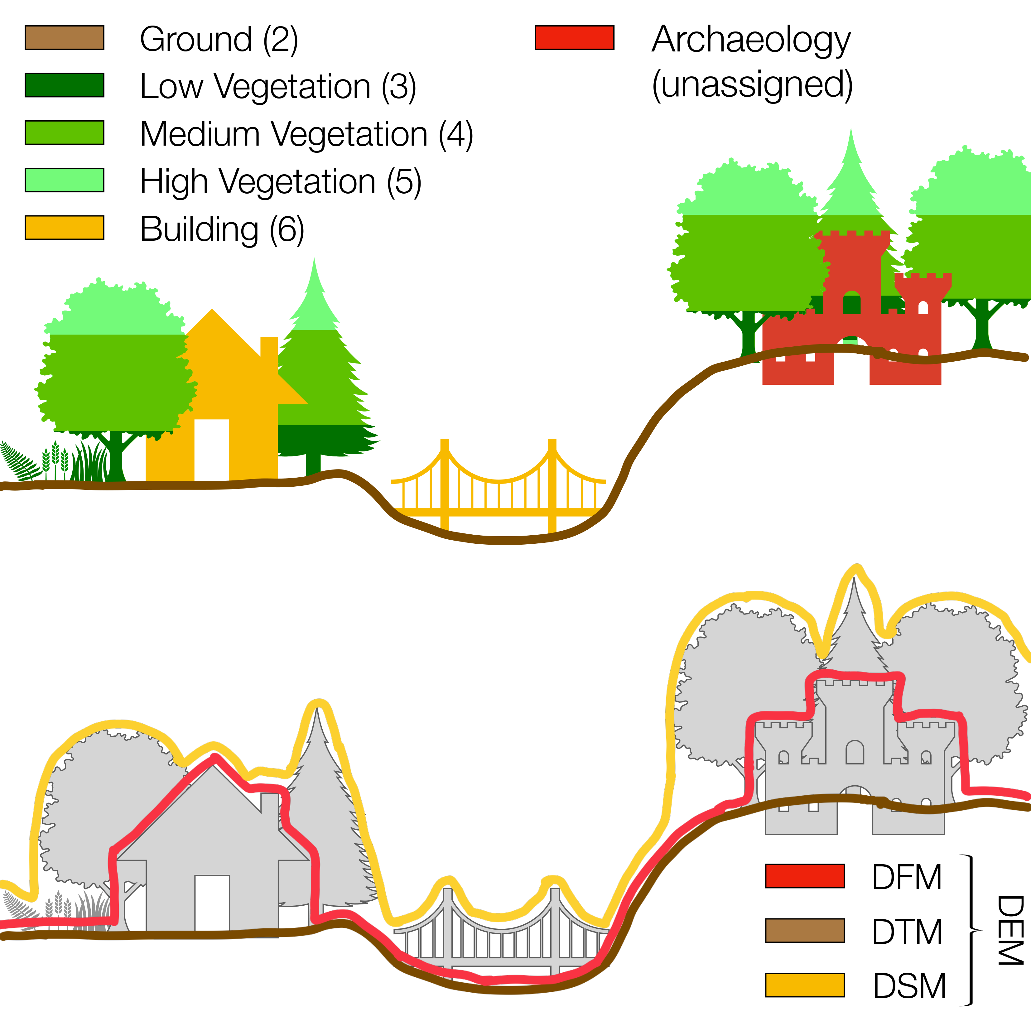
None of the above, however, describe an archaeology-specific gridded surface model. Archaeology-specific LiDAR data processing produces an archaeology-specific DEM. It combines ground data with archaeologically relevant micro-relief features or potential archaeological features: standing walls and stones, roads, channels, and earthworks [4]. Modern buildings are included to provide contextual information during the process of interpretative mapping, and to expedite orientation in the field [7]. Such an “archaeological digital elevation model” [4] has been called a digital feature model (DFM; Figure 1) [33]. It should be mentioned that although DFMs are commonly used in archaeological practice, they are usually referred to either as DEMs, e.g., [34,35] or DTMs, e.g., [4,36].
DFMs, then, are by definition archaeology-specific, and thus require the attention of archaeologists. Accordingly, the first aim of this paper is to describe DFMs in detail. The second goal is to contribute to archaeology-specific LiDAR data processing by providing the pipeline and tools for the automatic precision assessment of DFMs, which we have named the DFM confidence map. The DFM confidence map provides metadata that is a necessary part of the workflow documentation [7], helps in the process of interpretative mapping, and also enables the determination of the appropriate DFM resolution. The latter is a theoretical task, and another area that is neglected in the archaeological literature. To accommodate it, we have adapted the structure of this paper by adding the Theory section.
2. Materials and Methods
2.1. Test Sites
Four test sites were selected in order to simulate the most common archaeological uses of airborne LiDAR data (Figure 2). Due to the availability of data and first-hand experience, all of the datasets are from Europe. For the comparison of the different steps of data processing, these are the same test sites we have already used and outlined in other studies [1,7]. The description of the test sites is therefore only briefly repeated.
The test data from Austria (AT), Slovenia (SI1, SI2), and Spain (ES) were selected based on their archaeological and morphological similarity. Each site has a hilltop settlement (archaeology), buildings (modern), vegetation on steep slopes, and sharp discontinuities. An additional test site (SI2) was selected as an example of relentlessly dense low vegetation. Each test site is 1000 × 1000 m, but only the most relevant windows are shown in figures. All datasets are from nationwide data acquisitions and are in the public domain under various licences. The main difference between them is the average point density (Table 1). Therefore, the datasets represent, high, medium, and low point density scenarios, respectively.
2.2. DFM Quality Assessment
The fact that significant areas of DFMs derived from airborne LiDAR data are interpolated from undersampled points has important implications for all subsequent steps in the workflow. Most vulnerable to these implications are interpretative mapping and certain methods of “deep” interpretation—for example, hydrological analysis. An experienced operator is able to visually identify undersampled areas and, to some extent, the severity of the undersampling. By observing undersampled areas, the interpolator, or at least the family of interpolators, can also be identified in most cases. However, in order to achieve the necessary scientific integrity for archaeological interpretation, the quality of the DFM must be quantified. Given the high internal variability of DFMs, quality assessment must be done on a cell-by-cell basis.
This can be achieved using classification and regression tree analysis (CART). CART is a technique used in data mining that is commonly used as a rule-based classification design. The output of a CART analysis is a set of logical if–then conditions that end in terminal nodes and predict the value of the response variable. These conditional rules can be implemented using map algebra to create a quality assessment map. CART analysis is commonly applied to remote sensing data because it makes no assumptions about input data or their statistical distribution, and is well suited for dealing with collinear datasets, outliers, and potentially insignificant predictors [37,38,39,40,41].
CART was successfully used to derive the DEM uncertainty prediction map. Bater and Coops used CART analysis and identified ground point density and slope as the two conditions that have the greatest impact on error when the DEM is interpolated from airborne LiDAR data. They also tested vegetation structure, but found that it had the least effect on prediction [40]. However, Montealegre and colleagues found slope to be the most important factor, and that land cover type had a significant effect on the quality of DEM in forests [41]. Simpson and colleagues further refined this by finding that accuracy in flat terrain is primarily influenced by dense understory vegetation, such as ferns and brambles. Specifically, the error was associated with the density of vegetation up to a height of 3.5 m [42]. However, vegetation height is specific to each case study, and in our tests the difference between 3.5 m and 2.0 m (ASPRS class 3, low vegetation, which is defined as being 0.5–2.0 m above ground) was negligible.
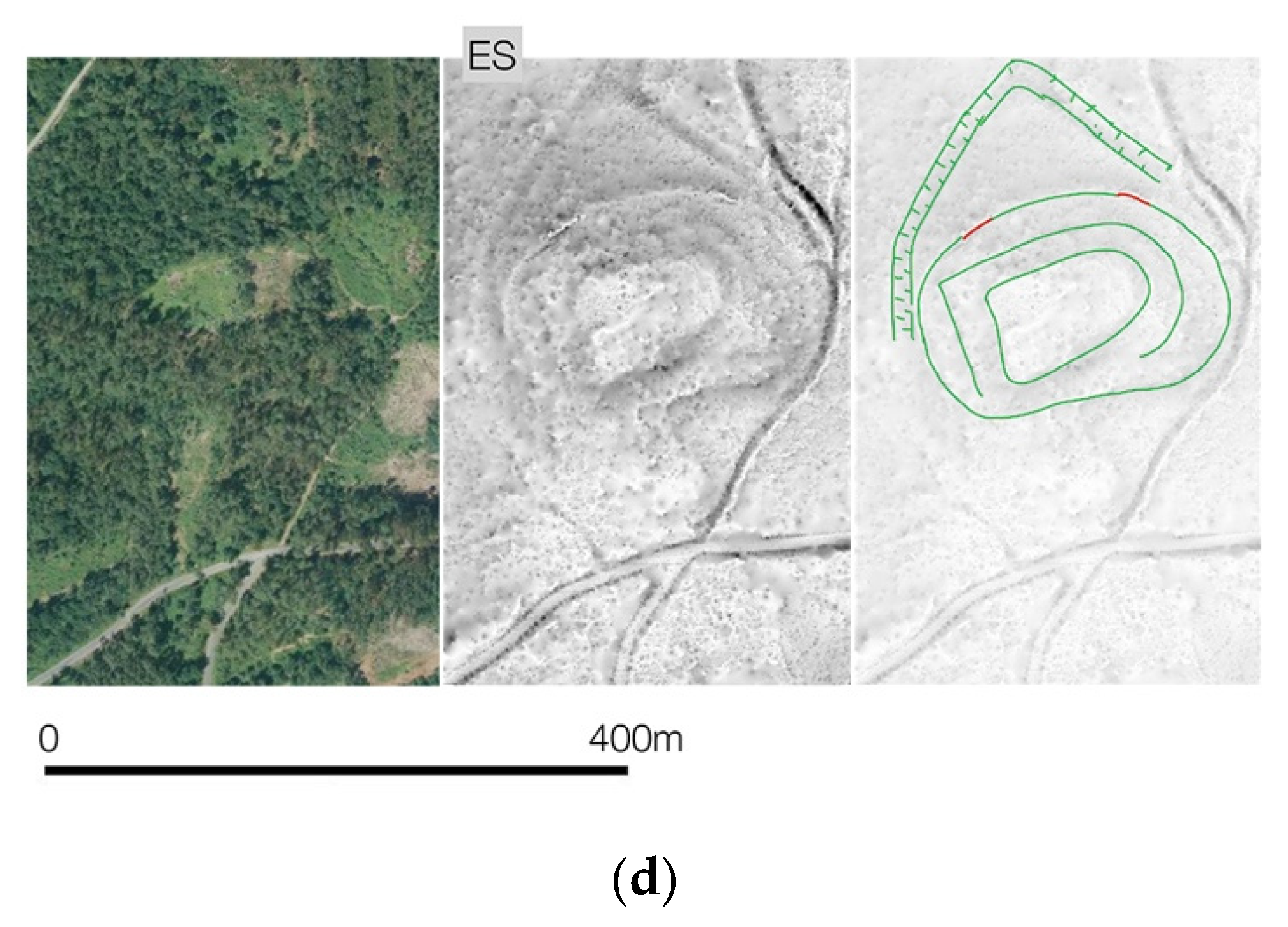
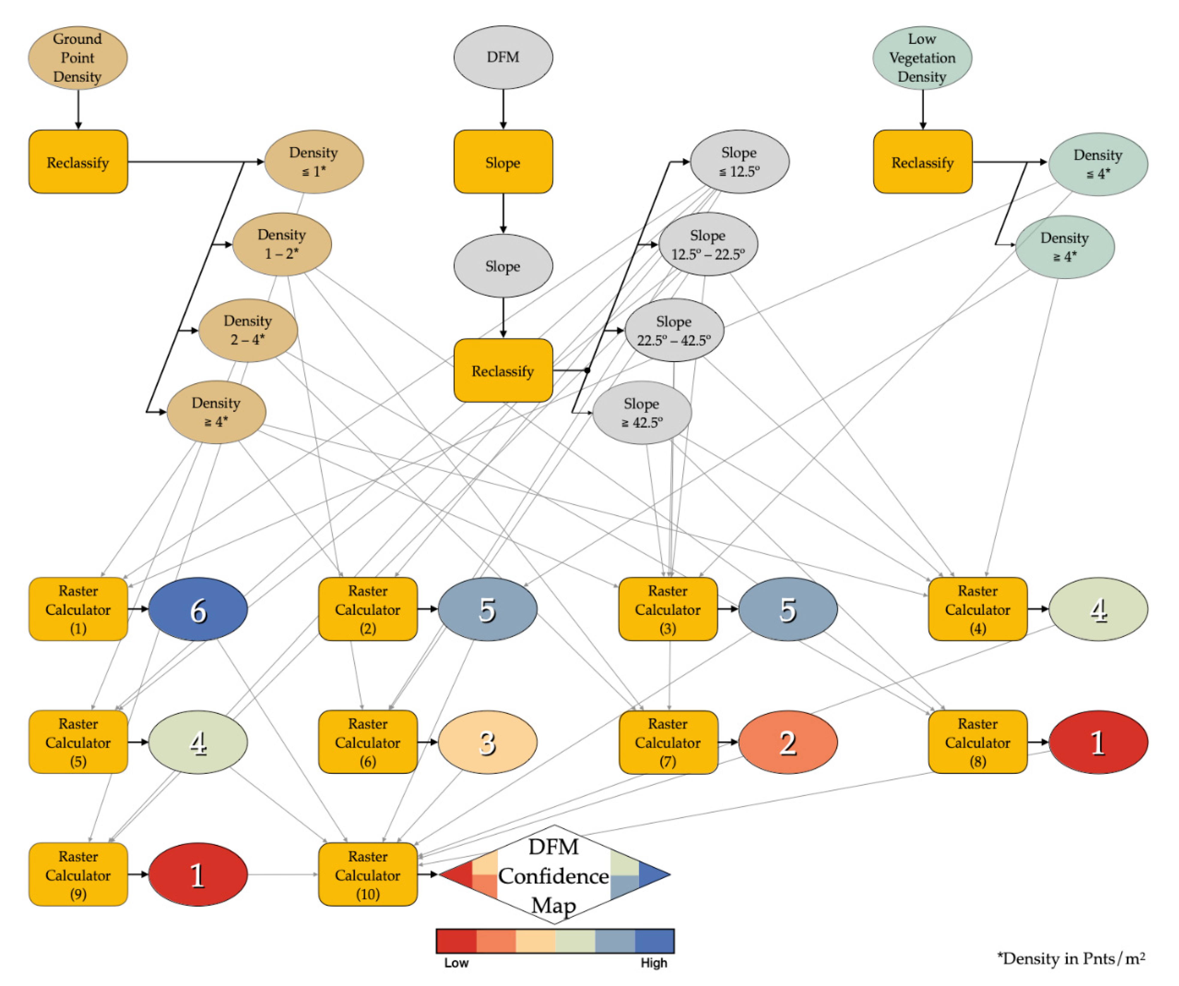
Therefore, we propose a modified CART classification tree with which to extract the DFM prediction uncertainty map, which we refer to as the DFM confidence map (Figure 3). Our CART tree is modelled after the proposal of Bater and Coops, who considered point density to be more important than slope. We modified the starting value for the ground point density according to the DFM specifications: The point density must be approximately equal to the grid density. The interpolator used is IDW. The slope conditions follow Bater and Coops, who defined thresholds at 12.5, 22.5, and 42.5°. To this, low vegetation was added following the decision tree structure of Montealegre and colleagues, but with vegetation height between 0.5 and 2.0 m. We defined the threshold for low vegetation density with the grid density: Vegetation is significant if its density is higher than the grid density, for example, more than 1 point per m2 for a grid cell size of 1 m2. This estimate roughly corresponds to a forest with a dense or very dense understory ([42]: structural categories C and D). The DFM confidence map has six confidence levels, with one being the lowest and six being the highest confidence.
We also provide visual precision testing of the DFM confidence maps. The accuracy of the DFM map is not questionable, since the method is derived from the statistical analysis of DEM accuracy tests [40,41,42]. More importantly, we argue that visual precision is more important for archaeology. Why? DEMs in general are used for analysis, visualization, or both [43]. Accuracy is the most important factor for analysis and precision of visualization. Since the primary application of DFMs in archaeology is visual analysis, precision is more important for us.
Our visual precision test of the DFM confidence maps was conducted by comparing DFM visual quality at different levels of confidence. The four test sites provide a good estimation of typical archaeological data at four levels of data quality.
2.3. Software Tool
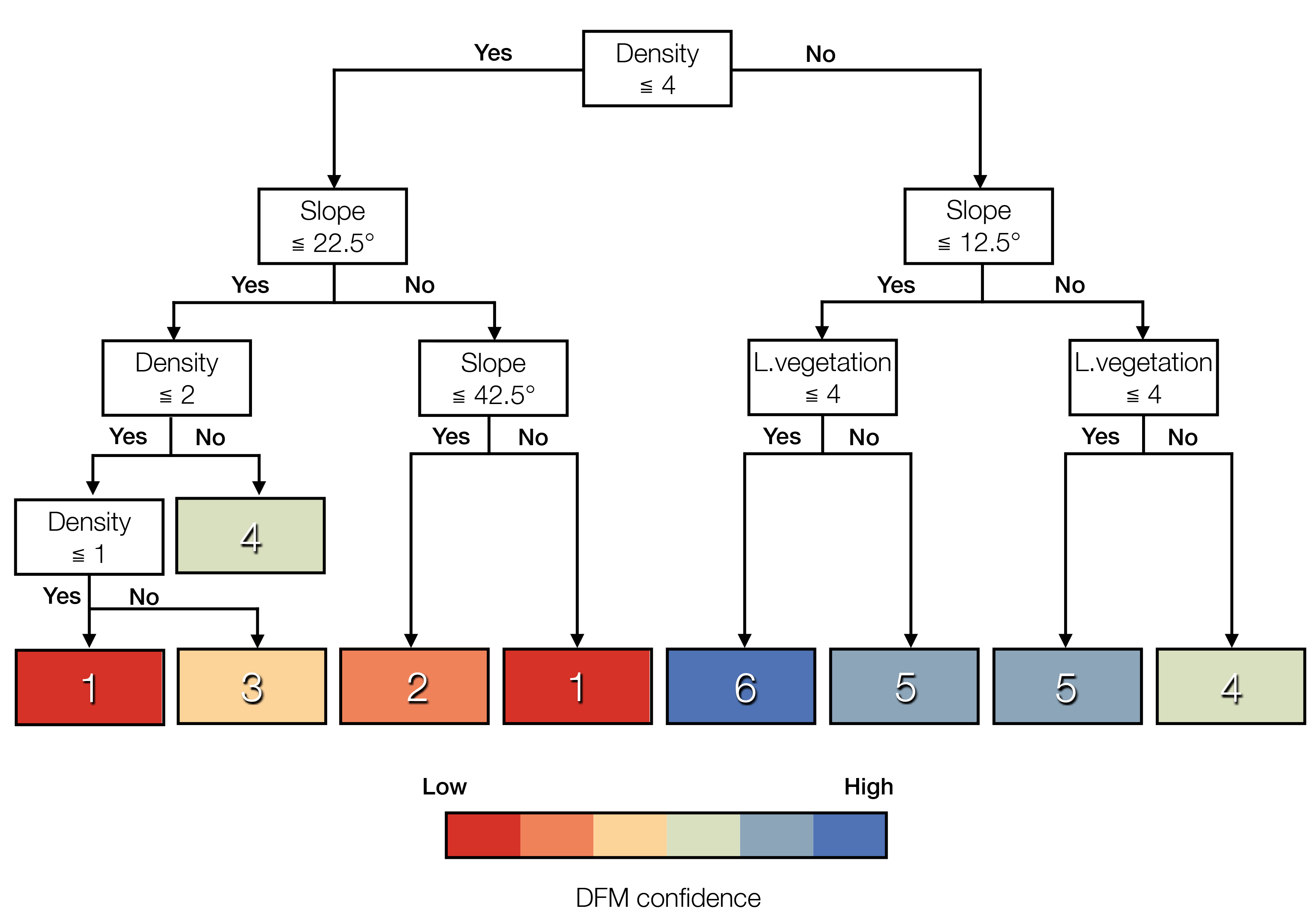
The tools required to compute a DFM confidence map—reclassification, slope, and raster calculator—are included in most GIS packages, and the process involves relatively low computational costs. However, the pipeline is relatively complex, consisting of 21 individual steps and 40 connections (Figure 4).
To facilitate the computation, we developed an open source tool in the form of a QGIS plug-in, which is available as a ZIP file via the Github repository [44]. In the first step, we built the pipeline in the QGIS graphical model designer. The first calculation uses the GRASS r.resample algorithm to unify the cell size (default 0.5 m) and the extent of the input rasters (DFM, vegetation density, and ground point density). The slope was then calculated using the QGIS slope algorithm. Each raster was then reclassified based on the above parameters or ranges using QGIS reclassify by table. The GDAL raster calculator was used to calculate the resulting confidence maps, which were styled according to the colour scheme introduced in this article (Figure 3 and Figure 4). The results were loaded as layers into QGIS. In the second step, the pipeline was implemented in the Python programming language to create a QGIS plug-in [45]. The plug-in has been tested in the latest long-term release of QGIS 3.16.x on Windows 10, macOS Big Sur, and Linux.
After installing the tool using the “Install from ZIP” dialog, the user first selects the input layers, either from files or from already loaded map layers. Depending on the options selected, the tool delivers up to four DFM confidence maps for resolutions of 0.25 m, 0.5 m (default), 1 m, and 2 m.
3. Theory
3.1. DFM
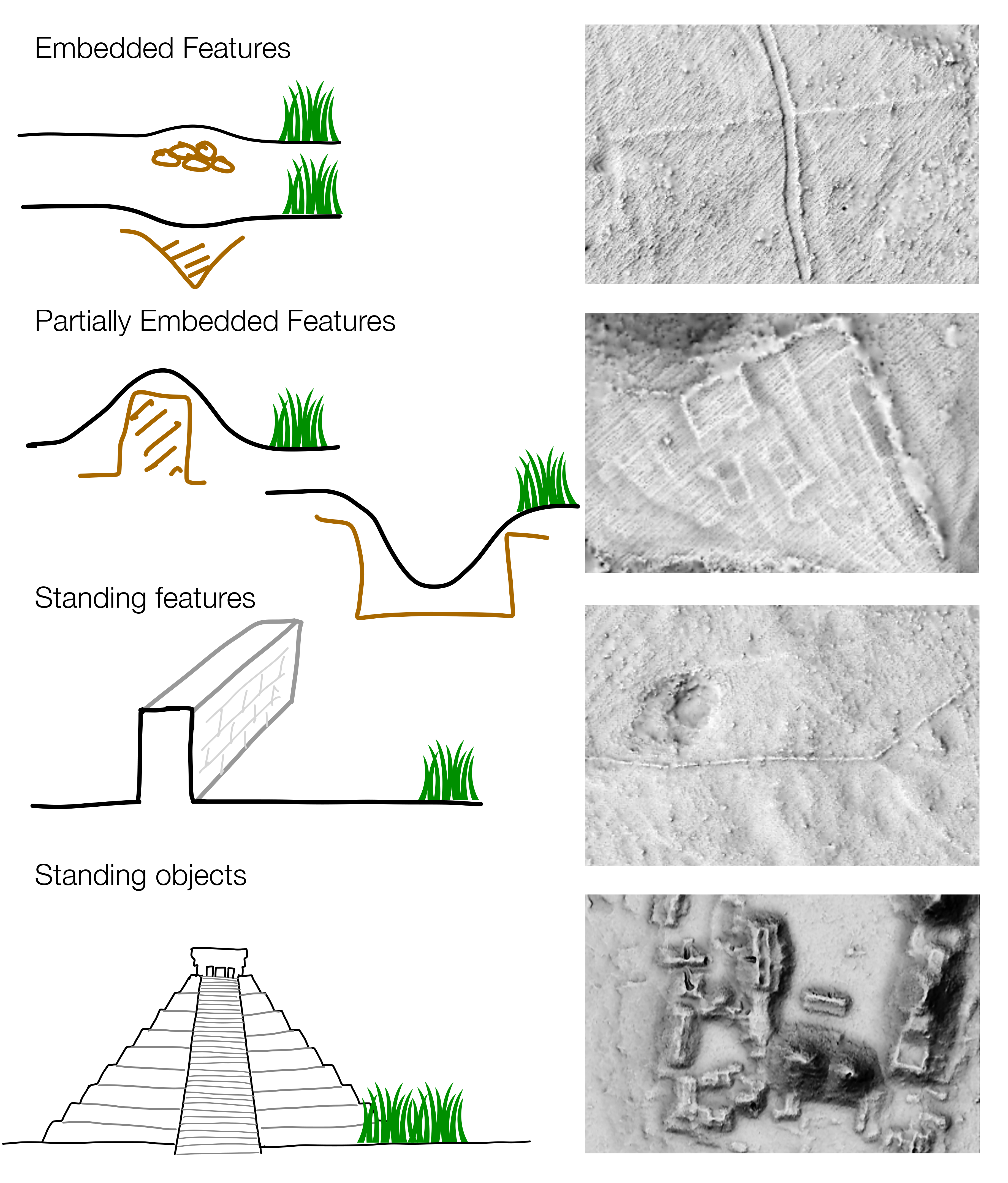
A DFM is an archaeology-specific gridded surface model—a product of archaeology-specific LiDAR data processing. It combines ground features with archaeological micro-relief features and buildings. To properly describe a DFM, therefore, archaeological features need to be specified. There are many different archaeological features, but four morphological types can be distinguished (Table 2; Figure 5). Most archaeological features detected using airborne LiDAR data fall into the first two types—embedded or partially embedded features—which are to some degree part of the ground and, hence, the DTM. This explains why archaeologists are able to detect many archaeological features using a general purpose DTM. However, standing features and standing objects are off-terrain features. As such, they are intentionally excluded from DTMs. In addition, partially embedded features may be misrepresented in a general purpose DTM because of smoothing or similar. Furthermore, while standing objects in point clouds can often be correctly classified using algorithms designed for buildings, there is currently no off-the-shelf solution for detecting standing features in areas with even modest low and medium vegetation (ASPRS classes 3 and 4, respectively). As a consequence, in many cases DFM-specific data processing must include ample manual reclassification [7].
It should be noted that standing features and standing objects are either relict (abandoned elements of earlier phases of landscape use that survive above ground) or fossilized features (elements of earlier phases of landscape use that are integrated into the later historic landscape, for example a linear earthwork re-purposed as a field boundary) [46].
We therefore use the term DFM as a subtype of DEM to describe the archaeology-specific gridded surface model of elevations that has been interpolated from ground points, buildings (ASPRS classes 2 and 6, respectively), and archaeological features.
3.2. Optimal DFM Resolution
In spatial sciences, the term “resolution” initially referred to the level of detail or to the smallest object that can be recognized on an aerial photograph. In a DEM or DFM, it refers to the grid cell size, and is expressed in terms of ground spacing. The smaller the grid size, the higher the resolution [47]. The selection of resolution is based on point density and distribution, horizontal accuracy, spatial autocorrelation, terrain complexity, or a combination of these. The computational cost and data storage should also be considered [48].
The first problem in generating a DEM is to determine a resolution that can represent the terrain features at the desired level of detail [49]. There are a number of studies on this topic, but they are field- and case-study specific (overview in [47]). For example, landscape scarps are identified on 1 m or 2 m DEMs [50], while a 10 to 30 m DEM is sufficient for an unbiased prediction of the landscape terrain [51]. There are no archaeology-specific studies that address the determination of the optimal resolution to represent the archaeological features that we are aware of. However, there have been several studies that have looked at point density. Two studies showed a significant improvement in point cloud classification success when the point density was increased from one to five data points per square meter (hereafter pnts/m2), and a slight improvement when the point density was further increased to 10 pnts/m2. It was the identification of the larger structures that benefited most from the increased resolution of the DEM [52,53]. In another study, the recognition rate of archaeological features was found to decrease slowly when the point density was reduced from 7.3 to 1.8 pnts/m2, and to decrease more rapidly with further reduction [54]. A Slovenian study demonstrated a decrease in the precision of DEMs when the pulse density was halved from 16 to 8 pulses per m2 [55]. A comparison of datasets at 0.7 and 2 pnts/m2 with a UAV dataset at 22 ground pnts/m2 showed little improvement in detection success [56]. Similarly, a comparison of a 0.5 pnt/m2 dataset with a 13 pnts/m2 dataset showed that the accuracy of archaeological interpretation was significantly better with the latter [57]. Some ongoing studies in Finland demonstrated stark improvement and numerous new features observed when comparing a 2 m DEM with 0.02 m and 0.1 m DEMs [58]. Based on these studies, we would cautiously agree that the effect of point density is not purely exponential, and that it has a breaking point at around 5 pnts/m2 [58] for most archaeological features that are not standing objects.
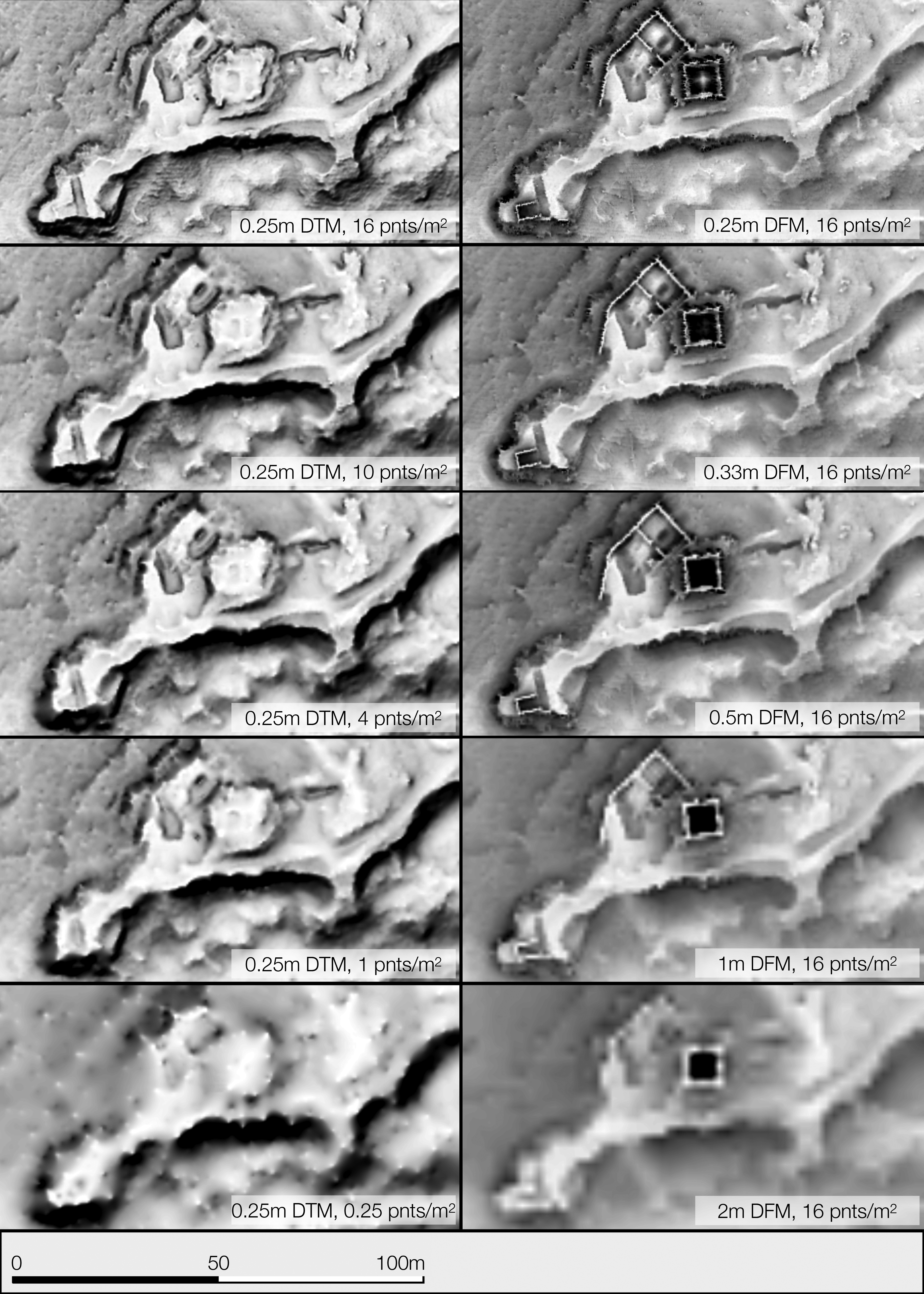
These results cannot be directly applied to DFM resolution. Both the reduction in point density and the reduction in DEM resolution have detrimental effects on visual precision, but the effects of each are very different. Our own experiment has shown that the amount of archaeological information deteriorates significantly when the resolution is reduced from 0.5 to 1 m (Figure 6).
This is consistent with the vast majority of published studies that use grids with 0.5 or 1 m resolution. Lower resolution is only used when better data are not available, and there are no examples that clearly show significant benefits of increasing resolution beyond 0.5 m. It can be said that 0.5 m DEM is currently the gold standard in archaeological practice. Archaeology-specific data acquisition is usually planned to produce a 0.5 m DFM or better. The types of archaeological features that can be recorded with such data can be estimated by applying the cardinal theorem of interpolation [59] and its implementation in archaeological field survey practice: The survey grid must be half the size of the archaeological features to be recorded. Therefore, current archaeological practice most commonly uses airborne LiDAR data to detect features either at least 1 m in diameter or linear features at least approximately 0.5 m wide. In practice, the most commonly acquired features are larger.
The second problem is determining the appropriate source data density. It is believed that for DEMs with lower resolution—for example, 5 m or lower—a point density as low as 0.36 points per grid cell may be sufficient [51]. For high-resolution DEMs, one point per grid cell is required [60]. Above this value, there is no appreciable improvement in accuracy [61]. On the other hand, if the point density is much lower, the surface will be representative of the specific interpolator used rather than the target terrain, because there will be many interpolation artefacts [62].
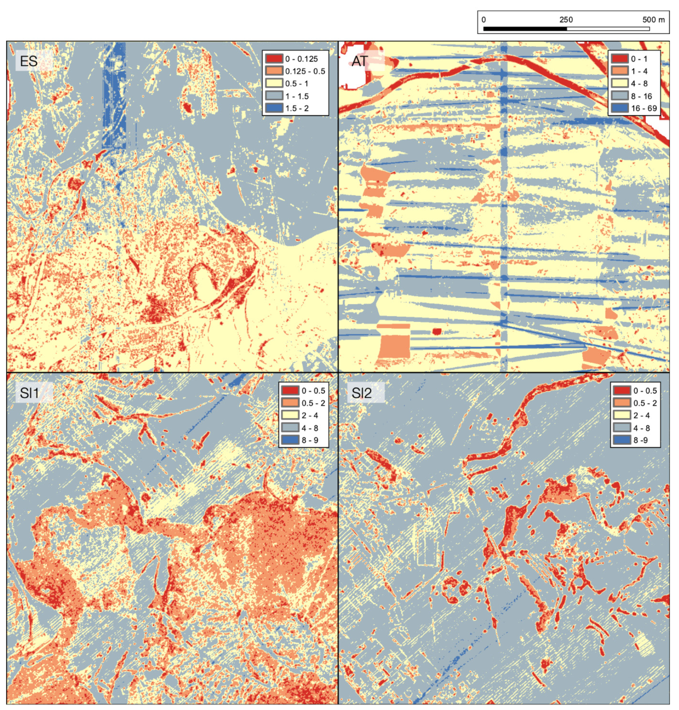
However, aside from data point density, there are several factors that affect the accuracy of DEMs: the morphology of the terrain, the interpolation method [63], and the distribution of the data points [64]. In the case of airborne LiDAR data, the latter is very important. This is because of non-uniform point distribution due to inter-scan-line spacing and flight strip overlap (Figure 7: AT) [20,65], and because data points are typically undersampled in non-vegetated areas and oversampled in densely vegetated areas (Figure 3: SI1 and SI2). This makes the typical airborne LiDAR data an inefficient data source, to say the least. For example, 4 pnts/m2 measured in a regular grid is a data source superior to a typical airborne LiDAR dataset with an average density of 4 ground pnts/m2. In a typical airborne LiDAR project, this fact is compensated for by brute force, so to speak—namely, by oversampling. In the above example, the LiDAR dataset would have to be densified to about 20 pulses/m2 in order to match the use case scenario of 4 manually measured ground pnts/m2.
However, many, if not most archaeologists use LiDAR data that have been acquired for non-archaeological purposes. For example, general purpose data are available for many countries and regions. For such projects, the question of resolution arises in reverse: How to determine the resolution that maximizes the use of the available data? The simplified answer is that the resolution should be approximately equal to the average point density; for example, a 0.5 m DFM should be interpolated if the data have 4 pnts/m2. For archaeology, a minimum of 2 pnts/m2 for a 0.5 m DFM is suggested [18]. However, as mentioned above, airborne LiDAR point data are extremely unevenly distributed. This is exacerbated to an extreme in terrain where densely forested steep slopes are mixed with fields and meadows interspersed with hedgerows. For example, in SI2 the density varies between 0.3 and 15 pnts/m2 within the boundaries of a single archaeological site, let alone a single 1 km2 tile (Figure 7: SI2).
4. Results
4.1. DFM Confidence Map
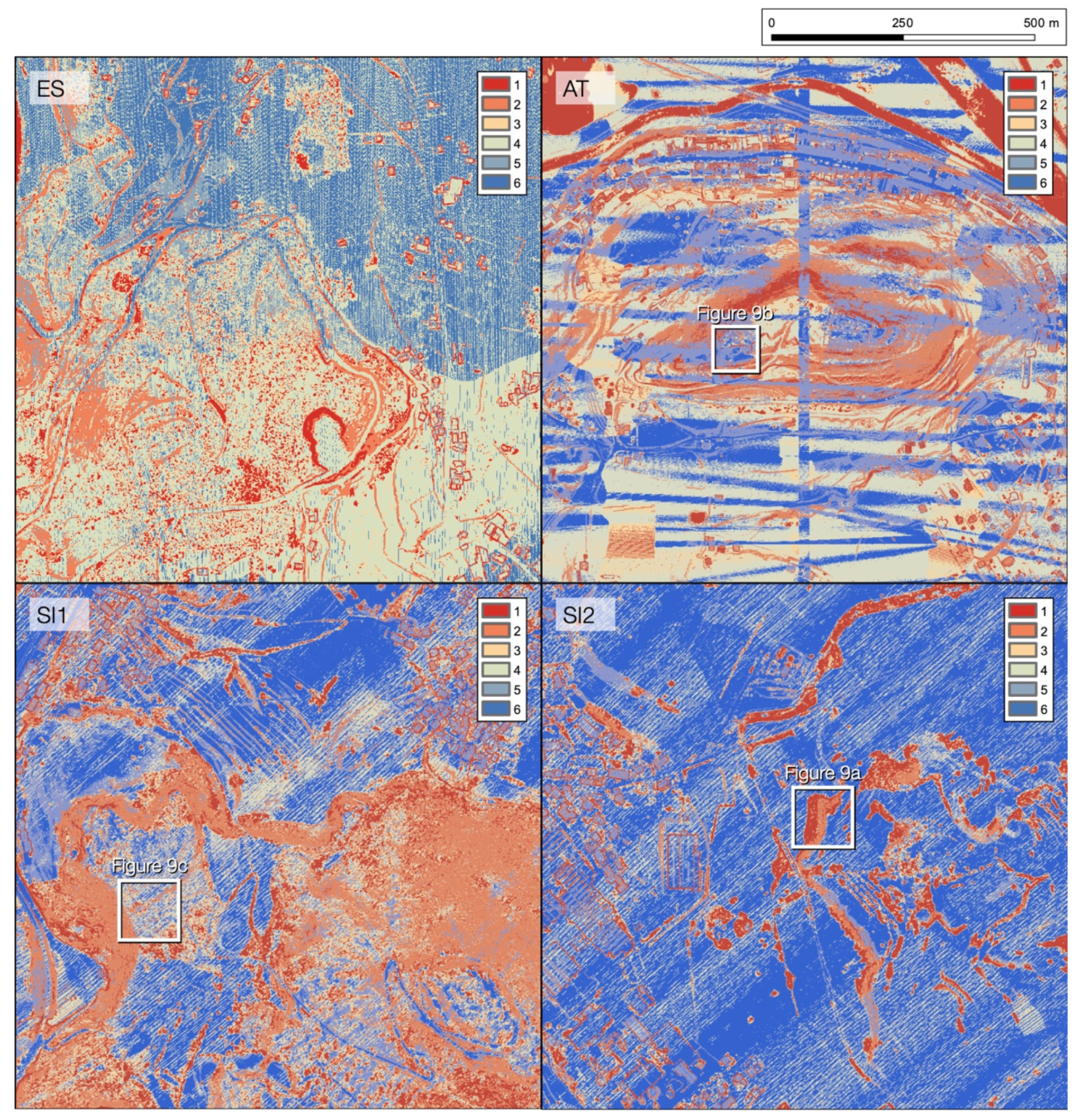
We have produced DFM confidence maps for each of our test sites at resolutions suitable to the data quality: 0.25 m for AT, 0.5 m for SI1 and SI2, and 1 m for ES (Figure 8). Looking at the structure of the maps it immediately becomes apparent that “orange” areas (confidence level two) are predominantly defined by steep slopes. As a consequence, these tend to appear in contiguous areas. Additionally, smaller—but still contiguous—“red” areas (confidence level one) that have been caused by dense vegetation or very low point density—for example, those caused by water bodies—are also apparent. These two landscape types are where the key differences between DFM confidence maps (Figure 7) and ground point density maps (Figure 6) appear. Other areas are often highly dispersed and directly comparable to ground point density.
We also tested the concordance of the DFM confidence map with visual precision assessment of DFM visualizations. For this we used the triangulated irregular network with linear interpolation (TLI) and sky view factor visualization (SVF). The TLI provides stark differences between undersampled and oversampled areas [66,67], while SVF is an established standard tool in archaeology [68].
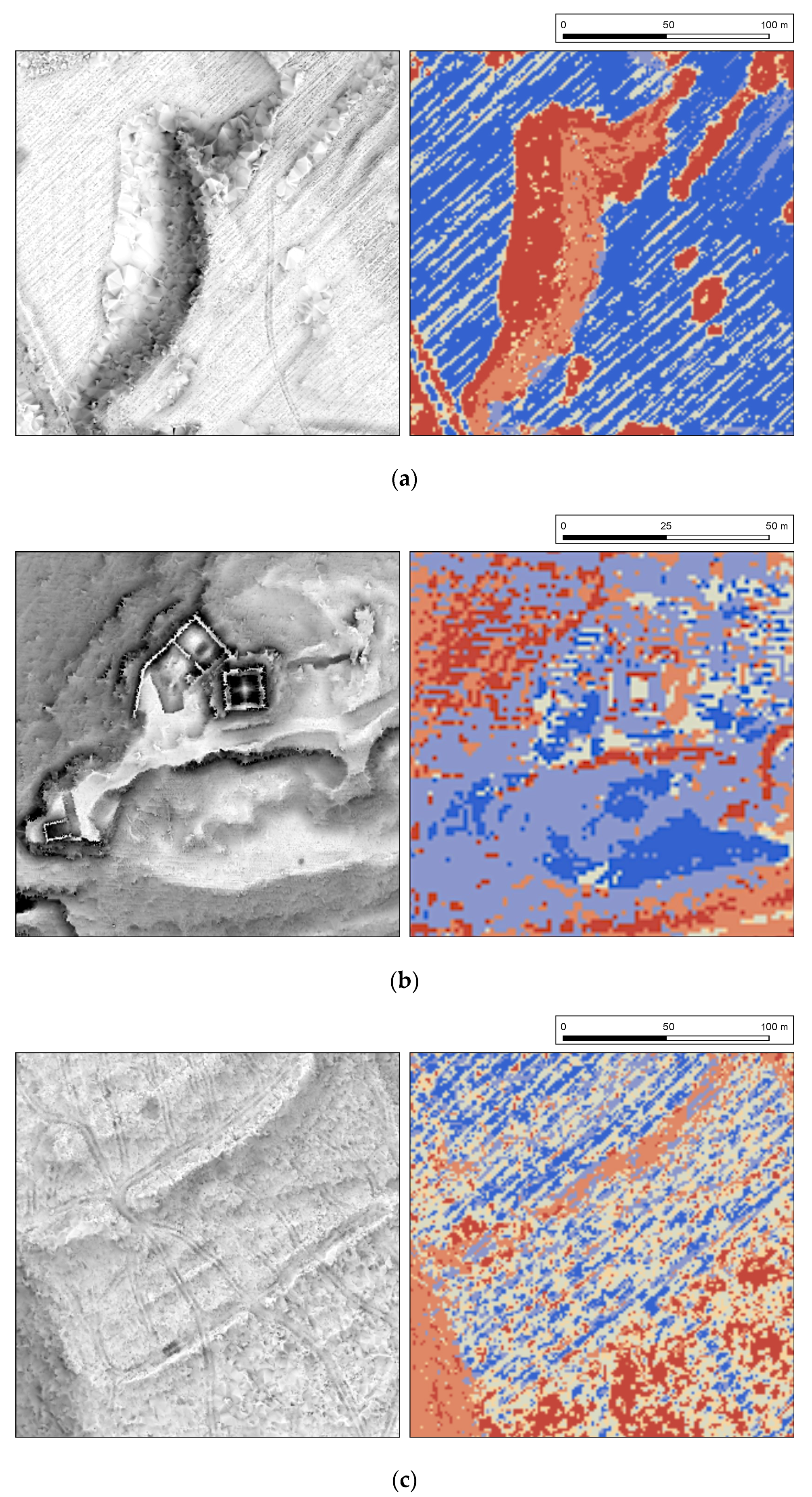
In “red” areas, the terrain could not be accurately predicted by any algorithm, and only algorithm artefacts were observed [62]—in this case, the triangular pattern. In “orange” areas this effect was still discernible (Figure 9a,b). Following the artefacts, both the “red” and the “orange” areas were a good match to the artefacts on the DFM. The same can be said for the “blue” areas (confidence levels five and six), which were perfect matches for the areas of highest visual quality (Figure 9b). “Transition” areas (confidence three and four) did not exhibit direct visual artefacts. However, looking at the selected features in detail confirmed the established confidence levels. We turned, for example, to the tracks left by heavy machinery clearing the forest after the ice rain disaster (Figure 9c). These tracks were about as wide as the size of the grid cell, but more pronounced than typical archaeological features. The fact that the tracks were not reproduced in full is proof that the quality of the DFM in that area was indeed not perfect, which is in line with confidence levels three and four.
We can therefore conclude that the visual assessment of the DFM confirms that the DFM confidence map is accurate in describing the DFM’s quality.
Obviously, the DFM confidence map has its limitations. The biggest problem with the CRAN method, as with any decision tree, is that it is based on binary decisions. In reality, for example, the quality of the DFM is not 15% worse at a slope of 12.4° than at a slope of 12.6°. Cell by cell, the method provides only rough estimates. However, when looking at a whole map—for example, a 1 km2 tile—it provides a good approximation and is an excellent indicator of the problem areas.
4.2. DFM Resolution
As mentioned, airborne LiDAR point data are extremely unevenly distributed, and it is difficult to determine optimal DFM resolution. There are several possible approaches to this [69]: (1) The conventional wisdom for DEM interpolation described above would suggest a grid resolution suitable for the vast majority of the dataset—for example, by fitting to the 95th percentile of point spacing in the dataset. The disadvantage is the loss of archaeological information in areas of locally high data density, such as meadows. (2) The second option is to segment the data into areas of similar point density, interpolate each area separately, and merge them for a final DEM. However, the result of this complex procedure would hardly differ from the simple (3) interpolation of the whole dataset with the resolution suitable for the areas with the highest continuous point density. The latter solution is more or less established in archaeological practice, mainly because of its practicality.
Archaeological DFMs are therefore interpolated at approximately the resolution corresponding to the areas with the highest continuous point density (not to be confused with the highest local point density, which occurs in narrow strips or small patches where flight lines overlap or intersect, respectively). Significant areas are therefore interpolated from undersampled points, making the choice of interpolator for archaeology much more important than in most LiDAR use case scenarios [70].
DFM confidence mapping can be used as a tool to determine the optimal DFM resolution. Based on the above results, and on our experience in interpretative mapping, ideally about ½ of the map should have a confidence level of three or four, and the remainder should be approximately evenly distributed among the other levels. However, if processing time and storage space are not limited, the resolution can be increased as long as at least one contiguous area of archaeological interest, such as a meadow complex, is level six.
5. Discussion and Conclusions
We set three goals for this work: to describe the archaeology-specific DFM in detail, to provide a tool for automatic precision assessment of the DFM, and to determine the suitable DFM resolution.
To date, very little attention has been paid to the specifics of archaeology-specific DEMs, although this has been a recurring topic in discussions at workshops and the like. Therefore, we first defined a DFM as a subtype of DEM, describing the archaeology-specific gridded surface model of elevations; this is interpolated from airborne LiDAR-derived ground points, buildings (ASPRS classes 2 and 6, respectively), and archaeological features. To achieve this, we defined for the first time the morphological types of archaeological features. This is not a trivial task, for two reasons: (1) there are a large number of archaeological features in different landscape contexts, and (2) with the increasing availability of hyper-resolution DFMs obtained via UAV–LiDAR, the list is likely to expand. We have therefore taken care to ensure that our definitions are broad enough to encompass all existing morphological types of archaeological features, and potentially those that we are not yet aware of.
The meaning of DFM, we believe, extends beyond the mere dictionary definition. It seems that the “revolution” that airborne LiDAR data have achieved in archaeology to date has been largely due to the enormous amount of archaeological information that has been obtained from general-purpose DEMs. This was possible because the vast majority of archaeological features are embedded features that form part of any general purpose DEM. We hope that these and other studies calling for archaeology-specific data processing will spur the next “evolutionary” step that will bring additional data by mapping archaeological features that can only be detected in DFMs. An accurate definition of DFMs is a prerequisite for an appropriate archaeology-specific data processing pipeline.
DFM quality assessment is a critical tool that enables such a processing pipeline. For example, DFM interpolation has not yet been addressed. Archaeologists have previously used tools and processing pipelines developed for DEMs or DSMs. IDW has been suggested as one of the more suitable interpolators for both, and the same is true for DFMs. However, IDW power variable two is best for DSMs and power three for DEMs [41]. Which is best for DFMs? Which has been used most often by archaeologists?
We do not provide answers to these questions in this paper, but we do provide the tools to answer them. The DFM confidence map is a tool (QGIS plug-in: [44]; see Supplementary Materials) for evaluating DFM quality. The primary application of the DFM confidence map is interpretive mapping, or the archaeological interpretation of DFMs. In particular, it allows the (automatic) determination of the confidence level for each mapped archaeological feature. This does not replace the confidence level determined by the operator, but can be used either in addition to it or as part of it. It also provides important metadata for interpretive mapping. For example, the density of a particular type of archaeological feature mapped in a given area may reflect past human activity, but it may also reflect bias in the data—e.g., fewer features in areas with a lower quality DFM—and such bias can be revealed by the DFM confidence map. In fact, any archaeological interpretation based on feature density and not matched with data quality (e.g., [71]) can be considered incomplete.
The third issue, which has been largely neglected in the archaeological literature, is the question of optimal DFM resolution. Regardless, in archaeological practice 0.5 m is an established gold standard. We have reasoned that the archaeology-specific optimal resolution should lean heavily towards undersampling in order to extract the maximum amount of archaeological information from a given dataset. The DFM confidence map can be used as a tool to determine the optimal DFM resolution. As defined above, the optimal archaeology-specific resolution for visualization will have a confidence level of three or four for approximately ½ of the map. If there are no computational cost constraints, the optimal resolution can be increased until at least one contiguous area remains at confidence level six, regardless of undersampling in other areas. DFMs intended for the analysis of GIS (or any DEM) will strive to be predominantly populated with confidence levels four or higher.
To this end, the DFM confidence map can serve another purpose: providing clear criteria for DEM or DFM segmentation into zones within which positioning accuracy assessment can be evaluated and reported. In this way, accuracy indices can be offered for each of the considered zones, which is one of the open issues in the field of DEM accuracy assessment [72] and interpolation.
We believe that these are all important steps towards a general methodological maturity of airborne LiDAR in archaeology, which is our ultimate goal.
Supplementary Materials
The QGIS plug-in is available online at https://github.com/stefaneichert/OpenLidarTools.
Author Contributions
Conceptualization, B.Š., E.L., and S.E.; methodology, B.Š.; software, S.E.; validation, E.L. and B.Š.; formal analysis, E.L.; writing—original draft preparation, B.Š. and E.L.; writing—review and editing, B.Š., E.L., and S.E.; visualization, E.L.; project administration, B.Š. and E.L.; funding acquisition, B.Š. All authors have read and agreed to the published version of the manuscript.
Funding
This research was funded by Slovenian Research Agency (ARRS) grant numbers N6-0132 and P6-0064, and Austrian Science Fund (FWF) grant number I 3992.
Institutional Review Board Statement
Not applicable.
Informed Consent Statement
Not applicable.
Data Availability Statement
Airborne LiDAR data for Slovenia are publicly available at http://gis.arso.gov.si/evode. Airborne LiDAR data for Spain are publicly available at http://centrodedescargas.cnig.es/CentroDescargas (accessed on 10 May 2021).
Acknowledgments
The authors give thanks for the constructive comments and suggestions by academic editors and the anonymous reviewers. Open Access Co-funding by the Austrian Science Fund (FWF).
Conflicts of Interest
The authors declare no conflict of interest. The funders had no role in the design of the study, in the collection, analyses, or interpretation of data, in the writing of the manuscript, or in the decision to publish the results.
References
- Štular, B.; Lozić, E. Comparison of Filters for Archaeology-Specific Ground Extraction from Airborne LiDAR Point Clouds. Remote Sens. 2020, 12, 3025. [Google Scholar] [CrossRef]
- Cohen, A.; Klassen, S.; Evans, D. Ethics in Archaeological Lidar. J. Comput. Appl. Archaeol. 2020, 3, 76–91. [Google Scholar] [CrossRef]
- Chase, A.S.Z.; Chase, D.; Chase, A. Ethics, New Colonialism, and Lidar Data: A Decade of Lidar in Maya Archaeology. J. Comput. Appl. Archaeol. 2020, 3, 51–62. [Google Scholar] [CrossRef]
- Doneus, M.; Mandlburger, G.; Doneus, N. Archaeological Ground Point Filtering of Airborne Laser Scan Derived Point-Clouds in a Difficult Mediterranean Environment. J. Comput. Appl. Archaeol. 2020, 3, 92–108. [Google Scholar] [CrossRef] [Green Version]
- Crutchley, S. Light Detection and Ranging (Lidar) in the Witham Valley, Lincolnshire: An Assessment of New Remote Sensing Techniques. Archaeol. Prospect. 2006, 13, 251–257. [Google Scholar] [CrossRef]
- Challis, K.; Carey, C.; Kincey, M.; Howard, A.J. Assessing the Preservation Potential of Temperate, Lowland Alluvial Sediments Using Airborne Lidar Intensity. J. Archaeol. Sci. 2011, 38, 301–311. [Google Scholar] [CrossRef]
- Lozić, E.; Štular, B. Documentation of Archaeology-Specific Workflow for Airborne LiDAR Data Processing. Geosciences 2021, 11, 26. [Google Scholar] [CrossRef]
- Menéndez Blanco, A.; García Sánchez, J.; Costa-García, J.M.; Fonte, J.; González-Álvarez, D.; Vicente García, V. Following the Roman Army between the Southern Foothills of the Cantabrian Mountains and the Northern Plains of Castile and León (North of Spain): Archaeological Applications of Remote Sensing and Geospatial Tools. Geosciences 2020, 10, 485. [Google Scholar] [CrossRef]
- Inomata, T.; Triadan, D.; Vázquez López, V.A.; Fernandez-Diaz, J.C.; Omori, T.; Méndez Bauer, M.B.; García Hernández, M.; Beach, T.; Cagnato, C.; Aoyama, K.; et al. Monumental Architecture at Aguada Fénix and the Rise of Maya Civilization. Nature 2020, 582, 530–533. [Google Scholar] [CrossRef] [PubMed]
- Stanton, T.W.; Ardren, T.; Barth, N.C.; Fernandez-Diaz, J.C.; Rohrer, P.; Meyer, D.; Miller, S.J.; Magnoni, A.; Pérez, M. ‘Structure’ Density, Area, and Volume as Complementary Tools to Understand Maya Settlement: An Analysis of Lidar Data along the Great Road between Coba and Yaxuna. J. Archaeol. Sci. Rep. 2020, 29, 102178. [Google Scholar] [CrossRef]
- Laharnar, B.; Lozić, E.; Štular, B. A structured Iron Age landscape in the hinterland of Knežak, Slovenia. In Rural Settlement: Relating Buildings, Landscape, and People in the European Iron Age; Cowley, D.C., Fernández-Götz, M., Romankiewicz, T., Wendling, H., Eds.; Sidestone Press: Leiden, The Netherlands, 2019; pp. 263–271. ISBN 978-90-8890-819-4. [Google Scholar]
- Stereńczak, K.; Zapłata, R.; Wójcik, J.; Kraszewski, B.; Mielcarek, M.; Mitelsztedt, K.; Białczak, M.; Krok, G.; Kuberski, Ł.; Markiewicz, A.; et al. ALS-Based Detection of Past Human Activities in the Białowiez a Forest-New Evidence of Unknown Remains of Past Agricultural Systems. Remote Sens. 2020, 12, 2657. [Google Scholar] [CrossRef]
- Evans, D. Airborne laser scanning as a method for exploring long-term socio-ecological dynamics in Cambodia. J. Archaeol. Sci. 2016, 74, 164–175. [Google Scholar] [CrossRef] [Green Version]
- Gheyle, W.; Stichelbaut, B.; Saey, T.; Note, N.; Van den Berghe, H.; Van Eetvelde, V.; Van Meirvenne, M.; Bourgeois, J. Scratching the Surface of War. Airborne Laser Scans of the Great War Conflict Landscape in Flanders (Belgium). Appl. Geogr. 2018, 90, 55–68. [Google Scholar] [CrossRef]
- Rosenswig, R.M.; López-Torrijos, R. Lidar Reveals the Entire Kingdom of Izapa during the First Millennium BC. Antiquity 2018, 92, 1292–1309. [Google Scholar] [CrossRef]
- Masini, N.; Lasaponara, R. On the Reuse of Multiscale LiDAR Data to Investigate the Resilience in the Late Medieval Time: The Case Study of Basilicata in South of Italy. J. Archaeol. Method Theory 2020. Available online: https://0-link-springer-com.brum.beds.ac.uk/article/10.1007%2Fs10816-020-09495-2 (accessed on 7 May 2021). [CrossRef]
- De Boer, A.G.; Laan, W.N.; Waldus, W.; Van Zijverden, W.K. LiDAR-based surface height measurements: Applications in archaeology. In Beyond Illustration: 2D and 3D Digital Technologies as Tools for Discovery in Archaeology; Frischer, B., Dakouri-Hild, A., Eds.; BAR International Series; Archaeopress: New York, NY, USA, 2008; pp. 76–84. ISBN 978-1-40730-292-8. [Google Scholar]
- Crutchley, S.; Crow, P. The Light Fantastic: Using Airborne Laser Scanning in Archaeological Survey; English Heritage: Swindon, UK, 2010. [Google Scholar]
- Doneus, M.; Briese, C. Airborne Laser Scanning in forested areas–Potential and limitations of an archaeological prospection technique. In Remote Sensing for Archaeological Heritage Management; Cowley, D.C., Ed.; Europae Archaeologia Consilium (EAC): Brussels, Belgium, 2011; pp. 59–76. [Google Scholar]
- Fernandez-Diaz, J.; Carter, W.; Shrestha, R.; Glennie, C. Now You See It … Now You Don’t: Understanding Airborne Mapping LiDAR Collection and Data Product Generation for Archaeological Research in Mesoamerica. Remote Sens. 2014, 6, 9951–10001. [Google Scholar] [CrossRef] [Green Version]
- Grammer, B.; Draganits, E.; Gretscher, M.; Muss, U. LiDAR-Guided Archaeological Survey of a Mediterranean Landscape: Lessons from the Ancient Greek Polis of Kolophon (Ionia, Western Anatolia). Archaeol. Prospect. 2017, 24, 311–333. [Google Scholar] [CrossRef] [PubMed] [Green Version]
- Kokalj, Ž.; Somrak, M. Why Not a Single Image? Combining Visualizations to Facilitate Fieldwork and On-Screen Mapping. Remote Sens. 2019, 11, 747. [Google Scholar] [CrossRef] [Green Version]
- Dong, P.; Chen, Q. LiDAR Remote Sensing and Applications; CRC Press, Taylor & Francis Group: Boca Raton, FL, USA; London, UK; New York, NY, USA, 2018; pp. 41–46. ISBN 978-1-4822-4301-7. [Google Scholar]
- Moore, I.D.; Grayson, R.B.; Ladson, A.R. Digital Terrain Modelling: A Review of Hydrological, Geomorphological, and Biological Applications. Hydrol. Process. 1991, 5, 3–30. [Google Scholar] [CrossRef]
- Doyle, F.J. Digital Terrain Models: An Overview. Photogramm. Eng. Remote Sens. 1978, 44, 1481–1485. [Google Scholar]
- Collins, S.H.; Moon, G.C. Algorithms for Dense Digital Terrain Models. Photogramm. Eng. Remote Sens. 1981, 47, 71–76. [Google Scholar]
- Podobnikar, T. Methods for Visual Quality Assessment of a Digital Terrain Model. SAPIENS 2009, 1, 1–10. [Google Scholar]
- Galin, E.; Guérin, E.; Peytavie, A.; Cordonnier, G.; Cani, M.-P.; Benes, B.; Gain, J. A Review of Digital Terrain Modeling. Comput. Graph. Forum 2019, 38, 553–577. [Google Scholar] [CrossRef]
- Demel, L.E.; Fornaro, R.J.; McAllister, D.F. Techniques for Computerized Lake and River Fills in Digital Terrain Models. Photogramm. Eng. Remote Sens. 1982, 48, 1431–1436. [Google Scholar]
- Lindsay, J.B.; Cockburn, J.M.H.; Russell, H.A.J. An integral image approach to performing multi-scale topographic position analysis. Geomorphology 2015, 245, 51–61. [Google Scholar] [CrossRef]
- ASPRS. LAS Specification Version 1.4-R13; The American Society for Photogrammetry & Remote Sensing: Bethesda, MD, USA, 2013. [Google Scholar]
- Miltiadou, M.; Campbell, N.D.F.; Cosker, D.; Grant, M.G. A Comparative Study about Data Structures Used for Efficient Management of Voxelised Full-Waveform Airborne LiDAR Data during 3D Polygonal Model Creation. Remote Sens. 2021, 13, 559. [Google Scholar] [CrossRef]
- Pingel, T.J.; Clarke, K.; Ford, A. Bonemapping: A LiDAR Processing and Visualization Technique in Support of Archaeology under the Canopy. Cartogr. Geogr. Inf. Sci. 2015, 42, 18–26. [Google Scholar] [CrossRef]
- Johnson, K.M.; Ouimet, W.B. Rediscovering the Lost Archaeological Landscape of Southern New England Using Airborne Light Detection and Ranging (LiDAR). J. Archaeol. Sci. 2014, 43, 9–20. [Google Scholar] [CrossRef]
- Rutkiewicz, P.; Malik, I.; Wistuba, M.; Osika, A. High Concentration of Charcoal Hearth Remains as Legacy of Historical Ferrous Metallurgy in Southern Poland. Quat. Int. 2019, 512, 133–143. [Google Scholar] [CrossRef]
- Doneus, M.; Kühteiber, T. Airborne laser scanning and archaeological interpretation–Bringing back the people. In Interpreting Archaeological Topography: Airborne Laser Scanning, 3D Data and Ground Observation; Opitz, R.S., Cowley, D.C., Eds.; Occasional Publication of the Aerial Archaeology Research Group; Oxbow Books: Oxford, UK, 2013; pp. 32–50. ISBN 978-1-84217-516-3. [Google Scholar]
- Bonham-Carter, G.F. Geographic Information Systems for Geoscientists: Modelling with GIS; Pergamon: Kidlington, UK, 1994; pp. 285–287. ISBN 978-0-08-041867-4. [Google Scholar]
- Lawrence, R.L.; Wright, A. Rule-Based Classification Systems Using Classification and Regression Tree (CART) Analysis. Photogramm. Eng. Remote Sens. 2001, 67, 1137–1142. [Google Scholar]
- Shao, Y.; Lunetta, R.S. Comparison of Support Vector Machine, Neural Network, and CART Algorithms for the Land-Cover Classification Using Limited Training Data Points. Isprs J. Photogramm. Remote Sens. 2012, 70, 78–87. [Google Scholar] [CrossRef]
- Bater, C.W.; Coops, N.C. Evaluating Error Associated with Lidar-Derived DEM Interpolation. Comput. Geosci. 2009, 35, 289–300. [Google Scholar] [CrossRef]
- Montealegre, A.; Lamelas, M.; Riva, J. Interpolation Routines Assessment in ALS-Derived Digital Elevation Models for Forestry Applications. Remote Sens. 2015, 7, 8631–8654. [Google Scholar] [CrossRef] [Green Version]
- Simpson, J.; Smith, T.; Wooster, M. Assessment of Errors Caused by Forest Vegetation Structure in Airborne LiDAR-Derived DTMs. Remote Sens. 2017, 9, 1101. [Google Scholar] [CrossRef] [Green Version]
- Ali, T.A. On the Selection of an Interpolation Method for Creating a Terrain Model (TM) from LIDAR Data. In Proceedings of the American Congress on Surveying and Mapping (ACSM) Conference 2004, Nashville, TN, USA, 19–21 April 2004. [Google Scholar]
- Eichert, S.; Štular, B.; Lozić, E. Open LiDAR Tools. Available online: https://github.com/stefaneichert/OpenLidarTools (accessed on 25 March 2021).
- Open Source Community 16.1.1. Writing a Plugin. PyQGIS Developer Cookbook. Available online: https://docs.qgis.org/3.16/en/docs/pyqgis_developer_cookbook/plugins/plugins.html#writing-a-plugin (accessed on 25 March 2021).
- Rippon, S. Historic Landscape Analysis: Deciphering the Countryside; Council for British Archaeology: New York, NY, USA, 2004. [Google Scholar]
- Xiaoye, L. Airborne LiDAR for DEM Generation: Some Critical Issues. Prog. Phys. Geogr. 2008, 32, 31–49. [Google Scholar] [CrossRef]
- Hengl, T. Finding the Right Pixel Size. Comput. Geosci. 2006, 32, 1283–1298. [Google Scholar] [CrossRef]
- Mitas, L.; Mitasova, H. Spatial Interpolation. In Geographical Information Systems: Principles, Techniques, Management and Applications, GeoInformation International; Longley, P., Goodchild, M.F., Maguire, D.J., Rhind, D.W., Eds.; Wiley: New York, USA, 1999; pp. 481–492. ISBN 978-0-471-73545-8. [Google Scholar]
- Chu, H.-J.; Wang, C.-K.; Huang, M.-L.; Lee, C.-C.; Liu, C.-Y.; Lin, C.-C. Effect of Point Density and Interpolation of LiDAR-Derived High-Resolution DEMs on Landscape Scarp Identification. Giscience Remote Sens. 2014, 51, 731–747. [Google Scholar] [CrossRef]
- Anderson, E.S.; Thompson, J.A.; Crouse, D.A.; Austin, R.E. Horizontal Resolution and Data Density Effects on Remotely Sensed LIDAR-Based DEM. Geoderma 2006, 132, 406–415. [Google Scholar] [CrossRef]
- Bollandsås, O.M.; Risbøl, O.; Ene, L.T.; Nesbakken, A.; Gobakken, T.; Næsset, E. Using Airborne Small-Footprint Laser Scanner Data for Detection of Cultural Remains in Forests: An Experimental Study of the Effects of Pulse Density and DTM Smoothing. J. Archaeol. Sci. 2012, 39, 2733–2743. [Google Scholar] [CrossRef]
- Ole Risbøl, O.M.B. Anneli Nesbakken Hans Ole Ørka Erik Næsset Terje Gobakken Interpreting Cultural Remains in Airborne Laser Scanning Generated Digital Terrain Models: Effects of Size and Shape on Detection Success Rates. J. Archaeol. Sci. 2013, 40, 4688–4700. [Google Scholar] [CrossRef]
- Trier, Ø.D.; Pilø, L.H. Automatic Detection of Pit Structures in Airborne Laser Scanning Data. Archaeol. Prospect. 2012, 19, 103–121. [Google Scholar] [CrossRef]
- Mlekuž, D.; Rutar, G. Koliko Točk? Gostota Lidarskih Snemanj Za Arheološke Prospekcije (How Many Points? Lidar Point Density in Archaeological Prospections). Arheo 2013, 30, 27–46. [Google Scholar]
- Risbøl, O.; Gustavsen, L. LiDAR from Drones Employed for Mapping Archaeology-Potential, Benefits and Challenges. Archaeol. Prospect. 2018, 25, 329–338. [Google Scholar] [CrossRef]
- Norstedt, G.; Axelsson, A.-L.; Laudon, H.; Östlund, L. Detecting Cultural Remains in Boreal Forests in Sweden Using Airborne Laser Scanning Data of Different Resolutions. J. Field Archaeol. 2020, 45, 16–28. [Google Scholar] [CrossRef]
- Risbøl, O.; Langhammer, D.; Mauritsen, E.S.; Seitsonen, O. Employment, Utilization, and Development of Airborne Laser Scanning in Fenno-Scandinavian Archaeology-A Review. Remote Sens. 2020, 12, 1411. [Google Scholar] [CrossRef]
- Shannon, C.E. A Mathematical Theory of Communication. Bell Syst. Tech. J. 1948, 27, 623–656. [Google Scholar] [CrossRef]
- McCullagh, M.J. Terrain and Surface Modelling Systems: Theory and Practice. Photogramm. Rec. 1988, 12, 747–779. [Google Scholar] [CrossRef]
- Liu, X.; Zhang, Z.; Peterson, J.; Chandra, S. The effect of LiDAR data density on DEM accuracy. In Proceedings of the MODSIM07: International Congress on Modelling and Simulation: Land, Water and Environmental Management: Integrated Systems for Sustainability, Christchurch, New Zealand, 10–13 December 2007; pp. 1363–1369. [Google Scholar]
- Albani, M.; Klinkenberg, B.; Andison, D.W.; Kimmins, J.P. The Choice of Window Size in Approximating Topographic Surfaces from Digital Elevation Models. Int. J. Geogr. Inf. Sci. 2004, 18, 577–593. [Google Scholar] [CrossRef]
- Aguilar, F.J.; Agüera, F.; Aguilar, M.A.; Carvajal, F. Effects of Terrain Morphology, Sampling Density, and Interpolation Methods on Grid DEM Accuracy. Photogramm. Eng. Remote Sens. 2005, 71, 805–816. [Google Scholar] [CrossRef] [Green Version]
- Gosciewski, D. Selection of Interpolation Parameters Depending on the Location of Measurement Points. Giscience Remote Sens. 2013, 50, 515–526. [Google Scholar] [CrossRef]
- Wehr, A. LiDAR Systems and Calibration. In Topographic Laser Ranging and Scanning: Principles and Processing; Shan, J., Toth, C.K., Eds.; CRC Press; Taylor & Francis Group: Boca Raton, FL, USA; New York, NY, USA; London, UK, 2018; pp. 159–200. ISBN 978-1-49-877227-3. [Google Scholar]
- Lee, D.T.; Schachter, B.J. Two Algorithms for Constructing a Delaunay Triangulation. Int. J. Comput. Inf. Sci. 1980, 9, 219–242. [Google Scholar] [CrossRef]
- Guibas, L.; Stolfi, J. Primitives for the Manipulation of General Subdivisions and the Computation of Voronoi Diagrams. ACM Trans. Graph. 1985, 4, 74–123. [Google Scholar] [CrossRef]
- Kokalj, Ž.; Zakšek, K.; Oštir, K. Application of Sky-View Factor for the Visualisation of Historic Landscape Features in Lidar-Derived Relief Models. Antiquity 2011, 85, 263–273. [Google Scholar] [CrossRef]
- Štular, B.; Lozić, E. Primernost podatkov projekta Lasersko skeniranje Slovenije za arheološko interpretacijo: Metoda in študijski primer (The Suitability of Laser Scanning of Slovenia Data for Archaeological Interpretation: Method and a Case Study). In Digitalni Podatki; Ciglič, R., Geršič, M., Perko, D., Zorn, M., Eds.; Geografski inštitut Antona Melika ZRC SAZU: Ljubljana, Slovenia, 2016; Volume 13, pp. 157–166. ISBN 978-961-254-929-9. [Google Scholar]
- Štular, B.; Lozić, E.; Eichert, S. Interpolation of Airborne LiDAR Data for Archaeology. HAL Preprints. 2021. Available online: https://hal.archives-ouvertes.fr/hal-03196185 (accessed on 16 April 2021).
- Canuto, M.A.; Estrada-Belli, F.; Garrison, T.G.; Houston, S.D.; Acuña, M.J.; Kováč, M.; Marken, D.; Nondédéo, P.; Auld-Thomas, L.; Castanet, C.; et al. Ancient Lowland Maya Complexity as Revealed by Airborne Laser Scanning of Northern Guatemala. Science 2018, 361, eaau0137. [Google Scholar] [CrossRef] [PubMed] [Green Version]
- Mesa-Mingorance, J.L.; Ariza-López, F.J. Accuracy Assessment of Digital Elevation Models (DEMs): A Critical Review of Practices of the Past Three Decades. Remote Sens. 2020, 12, 2630. [Google Scholar] [CrossRef]
Figure 1.
An outline of the differences between DEMs, DFMs, DTMs, and DSMs.

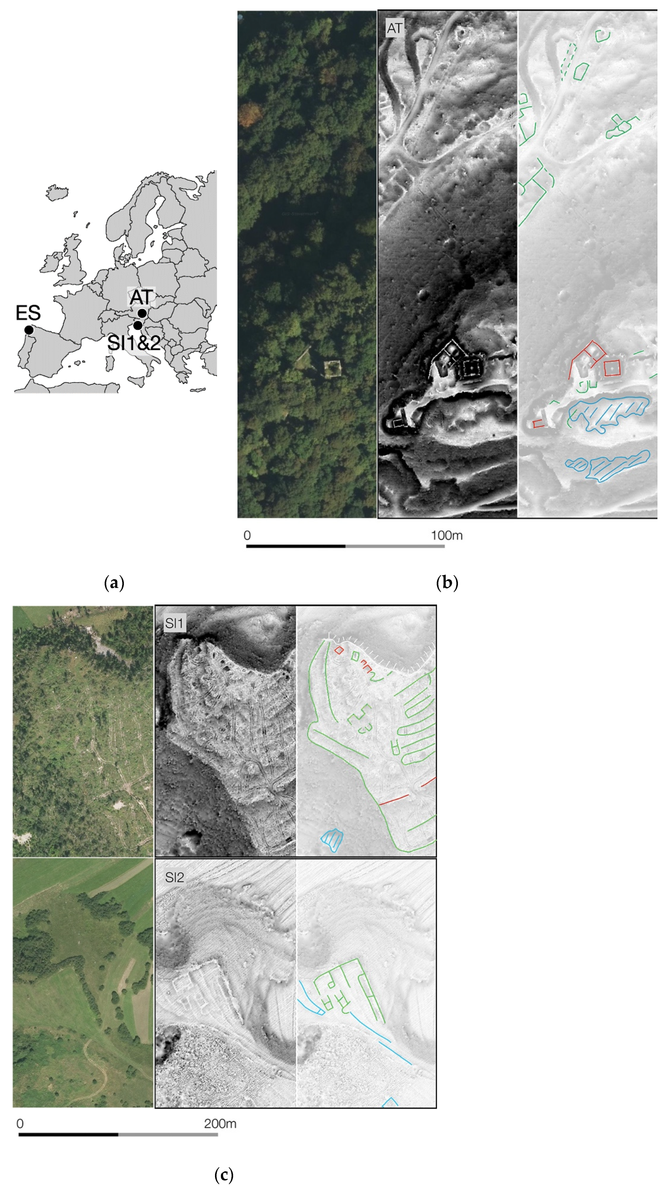
Figure 2.
Test data: (a) location of test sites: AT—46°53′05″N, 15°30′48′′E, SI1—45°40′21″N, 14°11′40′′E, SI2—45°40′56″N, 14°12′25″E, ES—42°44′30″N, 8°33′02″E; (b) test site AT; (c) test sites SI1 and SI2; (d) test site ES. (b–d): shown at 100% crop size; left-digital orthophoto; middle-enhanced visualization of manually processed DFM; right-archaeological features (blue: embedded features; green: partially embedded features; red: standing features). DFMs are visualised using sky view factor (RVT 2.2, default settings; after [1], Figure 1; CC-BY 4.0).


Figure 3.
Classification tree resulting from a CART analysis of absolute errors for 0.5 m DFM. The model is read from top to bottom until the terminal nodes, which predict the confidence level of the selected variables (one: lowest confidence; six: highest confidence).
Figure 3.
Classification tree resulting from a CART analysis of absolute errors for 0.5 m DFM. The model is read from top to bottom until the terminal nodes, which predict the confidence level of the selected variables (one: lowest confidence; six: highest confidence).

Figure 4.
Processing pipeline diagram for a 0.5 m DFM confidence map.

Figure 5.
Morphological types of archaeological features detectable via DFM (Bottom-right figure after [22], Figure 8, CC-BY 4.0).
Figure 5.
Morphological types of archaeological features detectable via DFM (Bottom-right figure after [22], Figure 8, CC-BY 4.0).

Figure 6.
Test site AT, the effects of reducing ground point density (left) and reducing DFM resolution (right). The ground point density and DEM/DFM resolution are indicated in each image. The processing pipeline is the same for all instances (point cloud processing according to [1]; OK interpolation; sky view factor visualization with default settings in RVT v.2.2). However, to demonstrate the effect of reduced point density on ground point filtering, the data in the left column lacks manual reclassification.

Figure 7.
Ground point density for each test site (in pnts/m2).

Figure 8.
DFM confidence maps for each test site (higher is better).

Figure 9.
Visualizations of DFMs (left) and DFM confidence maps (right) for selected areas at 200% crop size. See Figure 8 for the location. The processing pipeline is the same for all instances (point cloud processing according to [1]; TLI interpolation; 0.5 m DFM resolution; sky view factor visualization with default settings in RVT v.2.2).


Table 1.
Data point density for test sites. Pnts 106: No. of all data points in millions; Pnts/m2: median point density per m2 (average density is in this case equal to Pnts 106); Pnts 106 class 2&6: No. of points used for interpolation (ASPRS classes 2 and 6); Pnts/m2: median density of points used for interpolation per m2 (ASPRS classes 2 and 6); Spacing: average spacing between the points used for interpolation (ASPRS classes 2 and 6).
| Filter | Pnts 106 | Pnts/m2 | Pnts 106 (Class 2&6) | Pnts/m2 (Class 2&6) | Spacing (m) (Class 2&6) |
|---|---|---|---|---|---|
| AT | 12.11 | 15.54 | 7.52 | 8.96 | 0.33 |
| SI1 | 5.37 | 5.91 | 3.23 | 4.37 | 0.68 |
| SI2 | 5.39 | 5.81 | 4.65 | 5.23 | 0.62 |
| ES | 1.03 | 1.26 | 0.54 | 0.63 | 1.26 |
Table 2.
Morphological types of archaeological features typically represented in a DFM (after [1], CC-BY 4.0).
Table 2.
Morphological types of archaeological features typically represented in a DFM (after [1], CC-BY 4.0).
| Type | Description | Examples | DFM | DTM |
|---|---|---|---|---|
| Embedded f. | Slight positive or negative bulges typically with up to 0.5 m rise over 5 to 20 m run. | Trench, ditch, fossil field, past land division, track | Y | Y |
| Partially embedded f. | Positive or negative spikes typically with more than 0.5 m rise over 5 m run. | Dwelling, rampart, terrace, burial mound | Y | Y/N 1 |
| Standing f. | Off-terrain objects characterized by a sharp discontinuity in the ground. | Individual wall, castle ruins, collapsed building | Y | N |
| Standing objects | Large non-ground structures characterized by a sharp discontinuity in the ground and a significant diameter. | Mayan monumental architecture at Aguada Fénix, Khmer temples in Angkor | Y | N |
1 If the DTM is smoothened, which is often the case with general purpose airborne LiDAR derived DTMs, features may be diminished or even erased.
Publisher’s Note: MDPI stays neutral with regard to jurisdictional claims in published maps and institutional affiliations. |
© 2021 by the authors. Licensee MDPI, Basel, Switzerland. This article is an open access article distributed under the terms and conditions of the Creative Commons Attribution (CC BY) license (https://creativecommons.org/licenses/by/4.0/).
Share and Cite
MDPI and ACS Style
Štular, B.; Lozić, E.; Eichert, S. Airborne LiDAR-Derived Digital Elevation Model for Archaeology. Remote Sens. 2021, 13, 1855. https://0-doi-org.brum.beds.ac.uk/10.3390/rs13091855
AMA Style
Štular B, Lozić E, Eichert S. Airborne LiDAR-Derived Digital Elevation Model for Archaeology. Remote Sensing. 2021; 13(9):1855. https://0-doi-org.brum.beds.ac.uk/10.3390/rs13091855
Chicago/Turabian StyleŠtular, Benjamin, Edisa Lozić, and Stefan Eichert. 2021. "Airborne LiDAR-Derived Digital Elevation Model for Archaeology" Remote Sensing 13, no. 9: 1855. https://0-doi-org.brum.beds.ac.uk/10.3390/rs13091855
Note that from the first issue of 2016, this journal uses article numbers instead of page numbers. See further details here.