SNR-Based Water Height Retrieval in Rivers: Application to High Amplitude Asymmetric Tides in the Garonne River

Abstract

Signal-to-noise ratio (SNR) time series acquired by a geodetic antenna were analyzed to retrieve water heights during asymmetric tides on a narrow river using the Interference Pattern Technique (IPT) from Global Navigation Satellite System Reflectometry (GNSS-R). The dynamic SNR method was selected because the elevation rate of the reflecting surface during rising tides is high in the Garonne River with macro tidal conditions. A new process was developed to filter out the noise introduced by the environmental conditions on the reflected signal due to the narrowness of the river compared to the size of the Fresnel areas, the presence of vegetation on the river banks, and the presence of boats causing multiple reflections. This process involved the removal of multipeaks in the Lomb-Scargle Periodogram (LSP) output and an iterative least square estimation (LSE) of the output heights. Evaluation of the results was performed against pressure-derived water heights. The best results were obtained using all GNSS bands (L1, L2, and L5) simultaneously: R = 0.99, ubRMSD = 0.31 m. We showed that the quality of the retrieved heights was consistent, whatever the vertical velocity of the reflecting surface, and was highly dependent on the number of satellites visible. The sampling period of our solution was 1 min with a 5-min moving window, and no tide models or fit were used in the inversion process. This highlights the potential of the dynamic SNR method to detect and monitor extreme events with GNSS-R, including those affecting inland waters such as flash floods.

1. Introduction

The Global Navigation Satellite System (GNSS) has been used for decades for positioning and navigation purposes. Developments of GNSS constellations, more than twenty years ago, led to other remote sensing applications such as GNSS meteorology [1] and radio-occultation [2]. The L2 civilian (L2C) and L5 frequencies offer new tools for sensing atmospheric and Earth surface conditions; specifically, the L5 band improves altimetric performances of GNSS and Global Navigation Satellite System Reflectometry (GNSS-R) retrievals [3].

Recent developments include the improvements and use of GNSS-R as a consistent technique for retrieval of various land and ocean parameters. The operating principle for the use of these opportunistic signals was first proposed in 1988 [4], then experimented in 1993 for GPS constellation with an ocean altimetry case study [5]. These early experiments used a dual-antenna device, one up-looking to acquire the direct signal, and one down-looking to acquire the multipath reflected on the Earth’s surface. The use of a single geodetic antenna to combine both direct and reflected signals was introduced later [6]. The constructive and destructive interferences due to the coherent superposition of direct and reflected paths are transcribed in Signal-to-Noise Ratio (SNR) oscillations. This allowed successful retrieval of various environmental parameters such as soil moisture [7,8,9,10,11], snow depth [12,13], vegetation height [8,14,15] and, of course, ocean altimetry [16,17,18,19,20,21]. The technique is known as the Interference Pattern Technique (IPT), or GNSS Interferometric Reflectometry (GNSS-IR).

Nowadays, the ability and the interest of GNSS-IR to monitor sea level (SL) changes as a tide gauge is being assessed, especially in coastal areas where the capability of radar altimeters is limited, due to insufficient spatial and temporal sampling, and performance is degraded due to the presence of land contamination in the radar echo [22]. Nevertheless, some limitations of IPT were identified, mostly coming from the retrieval algorithms, especially when the tidal range was high. Most of the methods use a constant height assumption to retrieve the relative antenna height h, related to the frequency of the multipath oscillations [23]. As a consequence, water stages can be estimated only when the elevation rate ($\dot{h}$) is small, i.e., in micro to meso tidal conditions. The complete time series has to be reconstructed using a representation/interpolation of SL as a B-spline, tide models, or fitting a cubic spline on raw heights derived from SNR data [22]; a correction for the rate of change in SL is also necessary [17].

Few studies have been performed, to our knowledge, for retrieving water levels from GNSS-IR over rivers [24]. The major reason is the narrow width of rivers compared to the coastal ocean cases, which drastically limits the number of available reflections over the water surface. The majority of the SNR retrieval approaches only use low-elevation tracks to estimate the dominant frequencies [22], which are mainly masked or flagged in rivers. Some other reasons depend on the location of the study area along the river stream, presence of asymmetric tides in the downstream part of the rivers, occurrence of tidal bores at low tides and, for low-flow conditions over the same areas, occurrence of flash floods, which rapidly modify the river stage in the upstream part of the rivers. The constant height assumption [23] is not adapted to retrieve water levels during such complex and rapid phenomena. First the rate of elevation is higher, and asymmetry in tides prevents us from using models to estimate a correction based on the rate of change [17,25]. Pressure and acoustic measurements from the bottom of the river are commonly used to estimate water heights [26,27], and provide a consistent determination of tides. The case of tidal bores is more complicated, as they are highly nonhydrostatic phenomena, and pressure water levels are reconstructed under the hydrostatic assumption. Other instrumentation can help in better understanding the evolution of water levels and the spatial structure of tidal bores, i.e., GNSS measurements using a mobile antenna onboard a buoy [28], and LiDAR [27].

The dynamic SNR method was proposed to increase the range of applications of the IPT technique to all tidal environments, considering the vertical velocity of the reflecting surface (or elevation rate, $\dot{h}$) that is simultaneously estimated with the relative antenna height h using a Least Square Estimation (LSE) [29]. This allowed it to retrieve the temporal variations of the SL in macro-tidal environments (i.e., with a tidal range higher than 4 m) [19,29,30]. Furthermore, this method introduces a moving window to estimate dominant frequencies along the satellite tracks, while previous approaches estimate only one frequency per track at low elevations [22]. The use of the dynamic SNR method can provide more information when few GNSS satellite tracks are available, and integrates reflections from satellites with high elevation.

In this study, we analyzed SNR data acquired using a GNSS geodetic receiver on a platform over the Garonne River (France), 130 km upstream of its mouth, during one semidiurnal tide. The dynamic method was first used to retrieve the water levels. Due to the asymmetry of the tides and the complexity of the study area (small river, few GNSS satellites visible, vegetation on the riverbanks), it was adapted by introducing two processes for filtering the frequencies estimated with LSP before height inversion. Validation was performed using pressure water levels in the Garonne River.

2. Study Area and Datasets

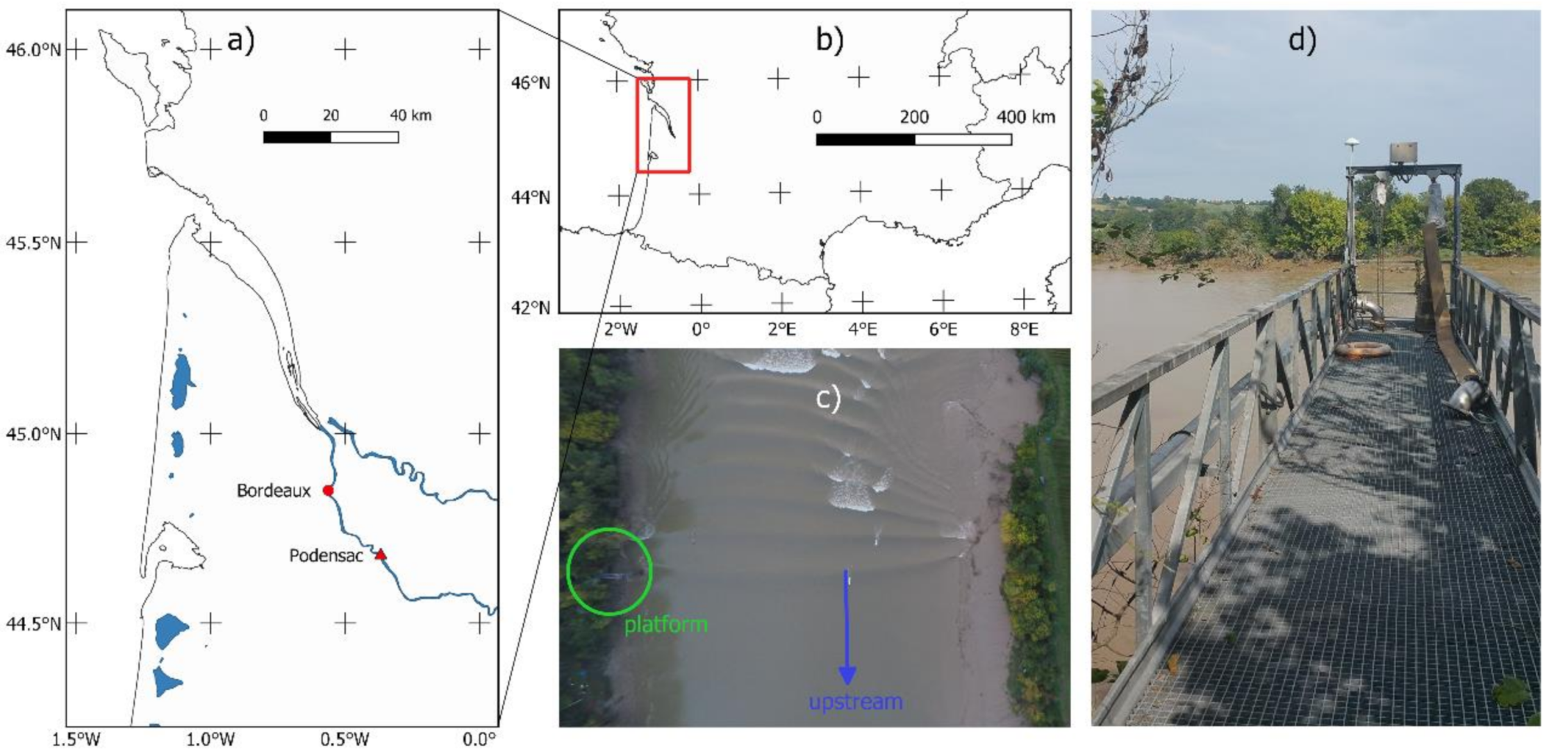
2.1. Study Area

The study area is located along the Garonne River in Podensac, southwest France (see Figure 1a,b). The confluence between the Garonne and Dordogne rivers forms the Gironde estuary in the Bay of Biscay. Tidal waves propagate in both rivers up to 160 km from the mouth of the estuary, with a tidal range exceeding 6m in Podensac [26,27]. Podensac is about 120 km upstream the mouth of the estuary and is the place where both the tidal range and the asymmetry of the tides are maximal due to a narrow river configuration.

Tides in alluvial estuaries, such as the Gironde/Garonne/Dordogne estuary, are highly asymmetric [27,31], unlike coastal areas where GNSS-R classical retrieval methods compare well to tide gauges [22]. While symmetrical patterns are found in most studies, asymmetric tides in Podensac compose a challenging dataset to explore the ability to retrieve high amplitude water level variations using GNSS-R. Rising tides last around three hours, while falling tides are slower, around nine hours, to complete a semidiurnal cycle. During faster rising tides, elevation changes materialized by the vertical velocity $\dot{h}$ reach 0.5 $\mathrm{mm}·{\mathrm{s}}^{-1}$ to 1$\mathrm{mm}·{\mathrm{s}}^{-1}$. Moreover, the Garonne River is affected by tidal bores, whose intensities are particularly high during spring tides combined with low discharge [26]. Extremely rapid variations of water height during this phenomenon (>1 $\mathrm{m}·{\mathrm{s}}^{-1}$ [27]) affect the performances of GNSS-R retrieval methods onsite. The structure of tidal bores is shown in Figure 1c. More information about the tides and the formation and dynamics of tidal bores in the Garonne and the Dordogne Rivers can be found in the literature [26,27,31].

The Garonne River in Podensac forms a straight line oriented from south-southeast (azimuth = 160°, upstream) to north-northwest (azimuth = 340°, downstream). The platform we used for SNR acquisition was on the left side of the river, whose width is around 150 m. We removed data in a 10° buffer corresponding to the potential interactions of reflected signals with the riverbank and the vegetation (including trees up to 20 m high: see Figure 1c,d). As no reflection was acquired on the north due to GPS orbits, the final azimuthal range was 10–150°. We also masked the data when elevation was below 5° (reflected signals affected by the vegetation on the opposite riverbank) or above 70° (reflections on the platform). These constraints drastically reduce the number of satellites tracked, and particularly the number of low-elevation tracks available for analysis.

2.2. GNSS-IR Data

A GNSS station composed of a conventional Leica AR10 antenna and GR25 receiver was installed on a platform above the river, ~4 m to 10 m above, depending on the tides (Figure 1d). It was used as a reference station to process the data acquired by a mobile GNSS receiver onboard a buoy using Differential GNSS (D-GNSS) technique, to retrieve water heights during tidal bore occurrence [28]. This reference station was also employed to collect SNR information at L1 (1575.42 MHz for GPS and 1602 MHz for GLONASS with a 562.5 kHz frequency shift between each carrier), L2 (1227.60 MHz for GPS and 1246 MHz for GLONASS with a 437.5 kHz frequency shift between each carrier), and L5 (1176.45 MHz for GPS) GNSS bands from GPS and GLONASS satellites reflected over the river.

The SNR acquisition was performed during a time span of 15 h, starting on October 17, 2016, at 2:35 p.m. UTC and ending on October 18, 2016, at 5:50 a.m. UTC. The nominal sampling rate was set to 20 Hz to further evaluate the ability of SNR-based retrieval methods to detect tidal bore propagation. A first tidal bore occurred on October 17th at 05:03 p.m., and a second on October 18th at 05:30 a.m. UTC (see Figure 2). In this study, we only focused on tide retrieval. Thus, 1 Hz resampled SNR data were used as inputs over the entire time span to retrieve the evolution of water heights during asymmetric tides. The output of our method produced a regularly spaced antenna height time series. Sampling was set to one minute for this case study.

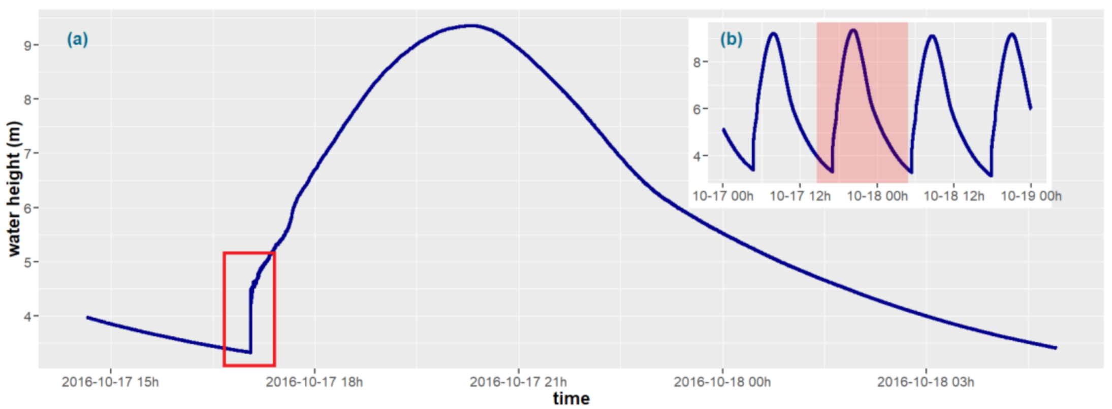
2.3. Validation: Pressure Data

Several instruments were installed on the riverbed from 12 October to 20 October 2016, to monitor tidal bore occurrences during spring tides, including an Acoustic Doppler Current Profiler (ADCP, Nortek Signature 1000) and a pressure sensor (Ocean Sensor Systems). Water heights estimated with pressure measurements using the hydrostatic assumption were used for comparison with the GNSS-R SNR height estimation (Figure 2). The specifications from the constructor indicated an accuracy of 0.05% on the pressure measurements, corresponding to an accuracy of about 0.005 m on the water height determination at high tides in Podensac. Nonetheless, the maximum error could reach up to 0.10 m in extreme conditions. The nominal sampling rate of pressure measurements was 10 Hz. For validation purposes, we smoothed the pressure water height while averaging values over a one minute interval to conform to the output sampling of GNSS-R height time series.

The whole anchorage containing the pressure and ADCP sensors was only referenced in longitude, latitude. No ellipsoidal height was provided, as it was installed to study temporal evolution of relative water height. For this reason, absolute comparisons between GNSS-R antenna heights and relative pressure water heights were impossible. Only relative comparisons, neglecting potential bias, were performed in this study.

3. Methods

3.1. Preprocessing

The SNR values represent the addition of the interferences of direct and reflected (multipath) signals components, which is written following [7]:

$$SN{R}^2=A_d^2+A_m^2+2A_d{A}_{m}cos\left(\psi \right),$$

(1)

where $A_d$ and $A_m$ are the amplitudes of the direct and multipath signals respectively, and ψ is the phase different between both signals. The term ${A_d}^2$ can be neglected since $A_m\ll A_d$ due to the attenuation upon reflection and the design of GNSS antennas. The direct component was modelled using a low-order polynomial function of elevation [23] then removed from the raw SNR time series. Here, as in most of the previous studies mentioned above, we used a 2nd order polynomial function. The remaining detrended SNR time series represents the multipath component corresponding to the reflected signals. Only specular points over the river were selected.

Due to the river characteristics in the study area (orientation and width, see Section 2.1), an azimuthal mask was applied to only select the tracks with an azimuth angle ranging from 10° to 150°. All elevation angles between 5° and 70° were retained, and higher values were masked by the platform on the top of which the antenna was installed. A small sample of reflected signals from low elevation could be affected by the presence of vegetation on the opposite riverbank. Nevertheless, we decided not to apply a more constraining mask on low elevations to maximize the number of available tracks for the inversion process.

Classical SNR-based retrieval methods use a limited elevation range (1–15°) to maximize the area of the first Fresnel zone [22]. This allows a more accurate height retrieval, as reflected signals are related to the crests of sea waves approximating a homogeneous surface. One frequency and height determination are performed for each single low-elevation track. In contrast, we used the dynamic SNR method [29] with a multisatellite approach, and no elevation mask was necessitated. This is a key point as very low-elevation tracks were not available due to vegetation masks and as we had a lesser number of satellites visible with constraining azimuthal configuration. We also performed a multifrequency analysis to improve the accuracy of the time series.

3.2. Dynamic SNR Inversion

According to [32], the multipath relative phase ψ of the detrended SNR time series is:

$$\psi =\frac{2\pi }{\lambda }\delta =\frac{4\pi h}{\lambda }sin\left(\epsilon \right)$$

(2)

with δ the path delay, λ the signal wavelength, ε the satellite elevation and h the receiver height. The frequency of the multipath oscillations can be obtained deriving Equation (2) against time [29]:

$$f=\frac{d\psi }{dt}=\frac{4\pi \dot{h}}{\lambda }sin\left(\theta \right)+\frac{4\pi h}{\lambda }cos\left(\theta \right)\theta \dot{}.$$

(3)

By making a change of variable $x=sin\left(\theta \right)$, we obtain:

$$\tilde{f}=\frac{d\psi }{dx}=\frac{4\pi }{\lambda }\left(\dot{h}\frac{tan\left(\theta \right)}{\theta \dot{}}+h\right).$$

(4)

The term with $\dot{h}$ can be neglected when $\dot{h}<1\times {10}^{-6} \mathrm{m}·{\mathrm{s}}^{-1}$ [23]. Equation (4) is then simplified and the dominant frequency $\tilde{f}$ is directly related to the antenna height h. This static case simplifies the computation assuming a very low elevation rate. In our case study, vertical velocities were much larger and the influence of the $\dot{h}$ component had to be considered.

Due to the characteristics of the study area, similar algorithms as the ones used for SL inversion (see [22] for a recent review) could not be used. Two main reasons constrained the retrieval of water heights with GNSS-R SNR in Podensac. First, the diurnal amplitude of the tides, which can reach up to 6 m, and the asymmetric tidal pattern, are responsible for high $\dot{h}$ especially during rising tides (see Figure 2), which is a major issue for most algorithms. Static SNR approaches applied to estimate SL use tide modelling to correct the $\dot{h}$ component or to reconstruct a complete time series from peaks and troughs (low $\dot{h}$). This is reliable when tides are symmetric, but not with asymmetric patterns. Second, the shape of the river in Podensac introduces a major constraint as reflections out of a 10–150° range fall out of the river (see Section 3.1). In most of the studies, the azimuthal range was near 360° and only observations with low elevations (<15°) were considered to maximize the extent of the first Fresnel zone and the accuracy of GNSS-R height retrieval. By contrast, in our study case it was mandatory to use a multisatellite, multielevation and multiGNSS frequency approach due to the lower number of available tracks.

The dynamic SNR method [29] offers an alternative technique which fits well with the problems we faced. A flowchart showing the initial method in blue, with our specific improvements in red, is presented in Figure 3. The basic idea was to estimate the dominant frequencies in a regularly spaced interval of time/elevation for all satellite tracks using a Lomb-Scargle Periodogram (LSP). These frequencies gathered into a moving window, filled an overdetermined system of equations following Equation (4), then h and $\dot{h}$ were jointly estimated using a Least Square Estimation (LSE, see Figure 3a). The parameter Δt, set by users, sampled the output time series of antenna heights by shifting the moving window in time. This approach was multisatellite because, from experience, the system of equations could only be solved if estimations from at least two distinct satellites were involved.

3.3. Improvements on the Dynamic SNR Approach

If we consider the dynamic approach as proposed by [29], the computed antenna heights exhibited very rough results (see Section 4.1). This was mainly due to the presence of noise in the dominant frequencies estimated using the LSP. As we considered the influence of $\dot{h}$ in the determination of $\tilde{f}$, a larger range of frequencies were analyzed. This may affect the quality of retrieved $\tilde{f}$ in several ways: low-frequencies due to the contribution of upper reflecting surfaces to the multipath signals (riverbanks, vegetation, the platform, boat stationed on the river) and high-frequency phenomena affecting the reflecting surface (tidal bores, boat wake: See Figure 1c). While the theoretical LSP outputs would present one single peak with high power, these aim to produce multi-peaks with equivalent power outputs, and a clear determination of the dominant frequencies is impossible. Illustrations of both a single peak and multipeaks outputs from LSP for the same satellite track are given in Figure 3b and Figure 3c respectively.

Enough tracks are needed to perform a dynamic SNR inversion, so the application of more constraining elevation masks is impossible, as this would remove a major part of the data. Instead, we propose a method to filter out the noisy dominant frequencies in two steps (see red charts in Figure 3a). First, we look to filter out all frequencies associated with multipeaks considered as not reliable. Let $\widetilde{f_a}$ be the main peak in LSP with power $P_a$. We consider $\widetilde{f_a}$ being a multipeaks output if a frequency $\widetilde{f_b}\ne \widetilde{f_a}$ is found with peak power $P_b$ that verifies:

$$P_b \ge k\times P_a,$$

(5)

with $0 \le k \le 1$. The value of parameter k is set empirically (see the results section). If k is low, a less noisy result is expected, but this may lead to gaps in the height determination. A 99% prediction interval (PI) is calculated based on single peak frequencies. This helps to extract the expected values in multipeaks LSP outputs and to fill the gaps resulting from filtering. If only one frequency is found in the PI, it is considered as the correct dominant frequency and extracted. In other cases, the multi-peaks are removed and a NA value is set at time index.

The second step consists of the implementation of an iterative least square approach to estimate h instead of the former single LSE estimation. It is necessary because of the persistence of noise after filtering out the multipeaks. For each iteration, approximated values of h and $\dot{h}$ are computed with LSE [29]. Corresponding approximate frequencies $f_{aprox}$ are calculated following Equation (4), and the standard deviation ${\sigma }_f=std\left(\tilde{f}-f_{aprox}\right)$ is deduced from initial and estimated frequencies. Absolute errors between $\tilde{f}$ and $f_{aprox}$ are calculated and $\tilde{f}$ is removed when:

$$\left|\tilde{f}-f_{aprox}\right|>3{\sigma }_f.$$

(6)

This corresponds to the filtering of the 1% worst values according to the Gaussian distribution. The standard deviation ${\sigma }_f$ decreases while iterating, and a convergence criterion is set on its value. This allows removal of most of the outliers, with successive estimations of the approximated values of h, $\dot{h}$ and $\tilde{f}$.

3.4. Validation

Pressure-derived water heights were used to validate the GNSS-R antenna heights. The absolute ellipsoidal height of the pressure sensor was not available which was the major issue in the validation procedure. Only a relative comparison between the dynamic SNR output and the pressure dataset was possible.

We further assumed that bias was zero, so the means of both datasets were adjusted for validation. Two metrics were then estimated: unbiased Root Mean Square Deviation (ubRMSD), adapted because of the no-bias assumption, and Pearson’s correlation coefficient (R). We compute ubRMSD and R for the entire water height time series, and we also calculated metrics on subsampled times series to study the influence of both the vertical velocity and the number of satellites visible on the SNR heights.

Following the adapted dynamic SNR algorithm, we retrieved 1-min regularly spaced time series of antenna heights using a 5-min moving window. To set the empirical parameter k, several determinations were performed ranging from k = 0.5 (high filtering of multipeaks) to k = 1 (no filtering case). Qualitative and quantitative conclusions are highlighted in the following section. Results for separate L1, L2, L5 and combination of GNSS bands are also presented.

4. Results

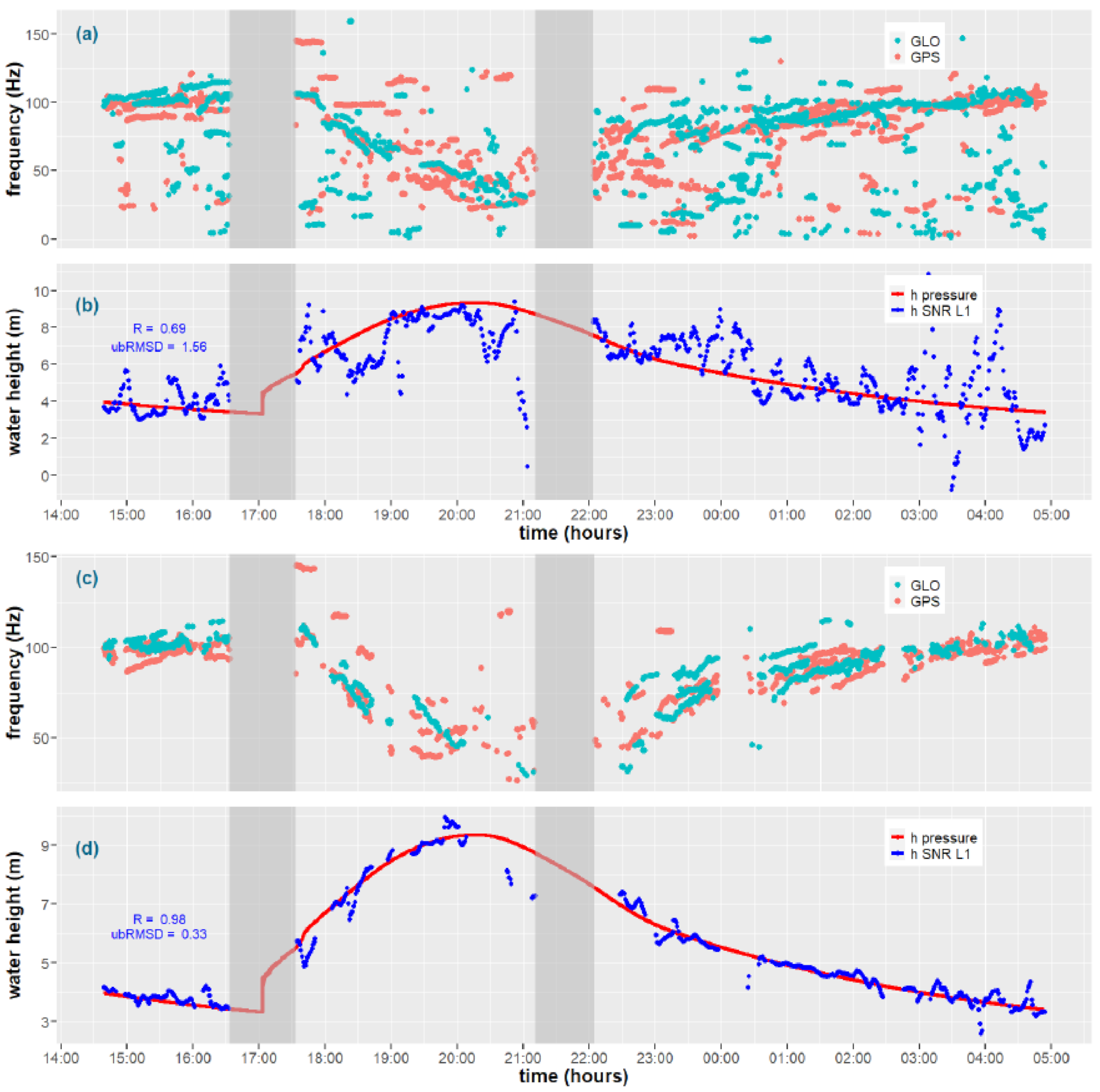
4.1. Preliminary Filtering of the Dominant Frequencies

The estimation and filtering of dominant frequencies is a key point of our method to reduce noise and achieve a convincing height inversion. A good estimation of parameter k is necessary to first reject massive multi-peak outputs in LSP, then the iterative LSE approach filters out remaining noise in the dominant frequencies. With k too low, the loss of information leads to gaps in the output or to a miscalculation of h. With k too high, the filtering of the noise would be insufficient and cause variability in the output time series. The optimal value of k was empirically determined. It depended on the environment, particularly on the variations of the reflecting surface, the width of the river and the high-frequency phenomena affecting the SNR time series. In our case, the combination of these factors required strong filtering.

Figure 4 presents the frequencies estimated before and after these two filtering operations for a L1-only retrieval. As the occurrence of tidal bores (here at ~5:03 p.m.) affects the frequency estimation in the moving window, we decided to remove estimations using a one hour buffer around the phenomena. The second gap from 9:00 to 10:00 p.m. was due to a stop in the acquisition recording.

Table 1. Performances of the adapted dynamic SNR inversion of h depending on the filtering level k, the minimal number of satellites, and the bands of frequency used. The best statistical results for each GNSS band/k parameter configuration were obtained with at least four satellites and new iterative LSE, while the worst results were obtained without the implementation of iterative LSE. Bold values highlight the best results for L1-only, L2-only and L1/L2/L5 height retrievals.

GNSS Bands Used	k	Iterative LSE	Min Number of Satellites	Nh—Number of deTerminations of h	Maximum Error (m)	R (Pearson)	ubRMSD (m)
L1	1	No	/	738	8.37	0.69	1.57
		Yes	2	735	10.45	0.73	1.64
			4	620	10.60	0.91	0.91
L1	0.90	No	/	733	3.82	0.90	0.85
		Yes	2	730	3.34	0.96	0.54
			4	643	3.32	0.97	0.47
L1	0.75	No	/	723	8.64	0.85	1.09
		Yes	2	720	8.46	0.88	0.96
			4	606	2.93	0.97	0.44
L1	0.60	No	/	715	20.64	0.83	1.19
		Yes	2	688	8.57	0.93	0.76
			4	529	1.59	0.98	0.33
L1	0.50	No	/	688	4.56	0.91	0.83
		Yes	2	660	5.28	0.93	0.72
			4	465	2.81	0.98	0.35
L2	0.60	No	/	702	21.60	0.77	1.48
		Yes	2	686	12.05	0.84	1.21
			4	476	1.59	0.99	0.32
L1, L2, L5	0.60	No	/	742	2.38	0.95	0.62
		Yes	2	741	2.16	0.98	0.44
			4	662	2.08	0.99	0.31

presents the statistical results obtained between each configuration of the adapted dynamic SNR algorithm (user-determined value of parameter k, GNSS bands used and minimal number of satellites for the inversion process) and the validation dataset. The values for R, ubRMSD, the maximum error and the number of points calculated with LSE using the configuration ($N_h$) are shown. Further analysis based on statistical values refer to this table.

The raw frequencies extracted with LSP (Figure 4a, with k = 1 and no iterative LSE process) show very noisy results particularly for the GLONASS constellation. The concordant estimation of h using LSE is fickle and highly affected by noise, as this is shown both graphically (Figure 4b) and statistically: R = 0.69, ubRMSD = 1.56 m, and the maximum error is 8.37 m. This presents the case of the nonadapted dynamic SNR method as proposed by [29] for SL retrieval. It confirms that the specific environment on rivers introduces noise in the SNR acquisition which has to be filtered. On the contrary, a much better result was observed with our adapted solution (Figure 4c), considering k = 0.6 and iterative LSE process with at least four satellites visible. The heights inverted using these filtered frequencies compared well to the reference (Figure 4d), with R = 0.98, ubRMSD = 0.33 m, with a maximum error of 1.59 m. All maximum errors listed in Table 1 are high but this was mainly due to a poor satellite configuration as we will discuss in Section 4.3 and Section 5.2.

The optimal k for the Podensac study case is 0.6 (Table 1). This value seems adapted to Podensac, but rivers with larger width, SL determinations and antenna configurations with a large azimuthal range should accommodate with a higher value of k tending towards 1 (no filtering case). Several determinations were made using the L1 GNSS band, while varying its value from 0.5 to 1 and with or without an iterative LSE approach. When k < 0.5 too many frequencies were filtered out so height inversion was affected. Results without iterative LSE implementation were systematically worse whatever the value of k. The influence of the minimal number of satellites will be presented and discussed later. Finally, when considering an iterative LSE approach to filter out noise, a high correlation and low ubRMSD were found for k = 0.9, k = 0.75, k = 0.6 and k = 0.5, with the best values obtained for k = 0.6. The maximum error also helped us in analyzing the results: the lower value was found for k = 0.6 (maximum error = 1.59 m), with much larger values for all other outputs (maximum error ≥ 2.81 m).

The two-step filtering method drastically improved the quality of the height retrieval. One last parameter should be considered too: the number of determinations of h ($N_h$), i.e., the number of systems of equations successfully resolved using LSE while shifting time (with the same sampling parameters for every time series). This informs the potential loss of data when the level of filtering is high. When compared to the no-filtering case (738 points), the best results using L1 for k = 0.9, k = 0.75, k = 0.6 and k = 0.5 had $N_h$ = 643 (87.1% of the total), $N_h$ = 606 (82.1%), $N_h$ = 529 (71.7%) and $N_h$ = 465 (63.0%), respectively. This highlights the cost of the filtering approaches, with only ~70% of the time series being calculated with the best parameters.

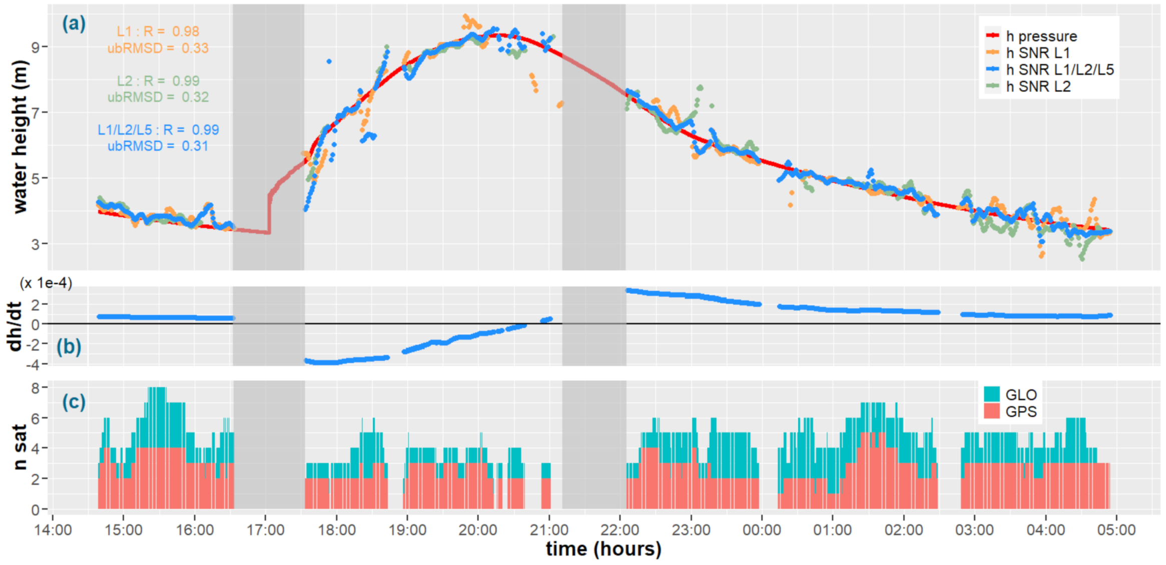
4.2. Comparison Between L1, L2 and L5 GNSS Frequencies

The first results were obtained using the GPS and GLONASS L1 frequency only. To ensure the stability of the solution, the L1 band was first chosen because few satellites during the acquisition (2016) also operated at the L5 frequency. The quality of SNR measurements from L2C is good [33,34], but few GPS satellites (from Block IIR-M, 2005) are equipped with it, and the L2 P(Y) code is more sensitive to noise due to weaker power. Furthermore, penetration of the L1 signal (λ = 0.1903 m) compared to L2 (λ = 0.2445 m) and L5 (λ = 0.2540 m) signals in the vegetated riverbanks may change due to the wavelength difference. To prevent effects on studying reflections from heterogeneous surfaces, we first did a band-by-band inversion then compared results to the multiband analysis. The respective performances of L1 and L2 bands for GNSS-R altimetry are a subject of discussion [34].

The interest of the technique was assessed using the L1 band only (Figure 4d). Figure 5 presents final results using all bands: joint estimation of h (Figure 5a) and $\dot{h}$ (Figure 5b), and number of distinct GPS and GLONASS to solve the system of equations (Figure 5c). Figure 5a also superimposes the L1 only, L2 only and L1 + L2 + L5 height retrieval with the reference time series. Extended statistical results are found in Table 1. A qualitative analysis highlights the consistency of all the solutions calculated. Single band time series (L1 in orange, L2 in green) look noisy, especially when few satellites were visible: at ~9:00 p.m. (L1), ~11:00p.m. (L2) or ~0:30 a.m. (L1). On the contrary, they correlated well to each other and to the all-band solution (in blue) when optimal conditions were found, i.e., a high number of satellites and a low $\dot{h}$: before 4:30 p.m., and from 0:30 a.m. to 2:30 a.m. Looking globally, the three-time series were comparable with a bias below 0.03 m, and the wavelength gap from L1 to L2 and L5 bands did not affect the height retrieval.

Statistical results led to comparable conclusions. The correlation coefficients R were greater than 0.98 for every time series, and ubRMSD ranges from 0.31 m to 0.35 m, the best performance being obtained using all bands. The maximum errors were comparable for L1 and L2 (1.59 m), and surprisingly larger for the all-bands solution (maximum error = 2.08 m). This corresponds in reality to individual noisy points when few satellites were visible, e.g., between 6:00 p.m. and 7:00 p.m. (see Section 5.2 for details). Using the L1 band only, we obtained $N_h$ = 535. Although presenting excellent statistical results, $N_h$ = 484 for the L2-only case, confirmed that the absence of the L2 civilian frequency for some GPS satellites led to data gaps, especially when few satellites were visible. Finally, when combining all the L1, L2 and L5 bands in a unique system of equations, $N_h$ = 664 was obtained. Compared to this result, the output time series of antenna height contained 19.4% fewer points for the L1-only case and 27.1% less for the L2, for quasi-identical statistical results. This loss of information was particularly accentuated when the configuration of the study area provided a restricted number of available satellite tracks for SNR based inversion, as in the Podensac case.

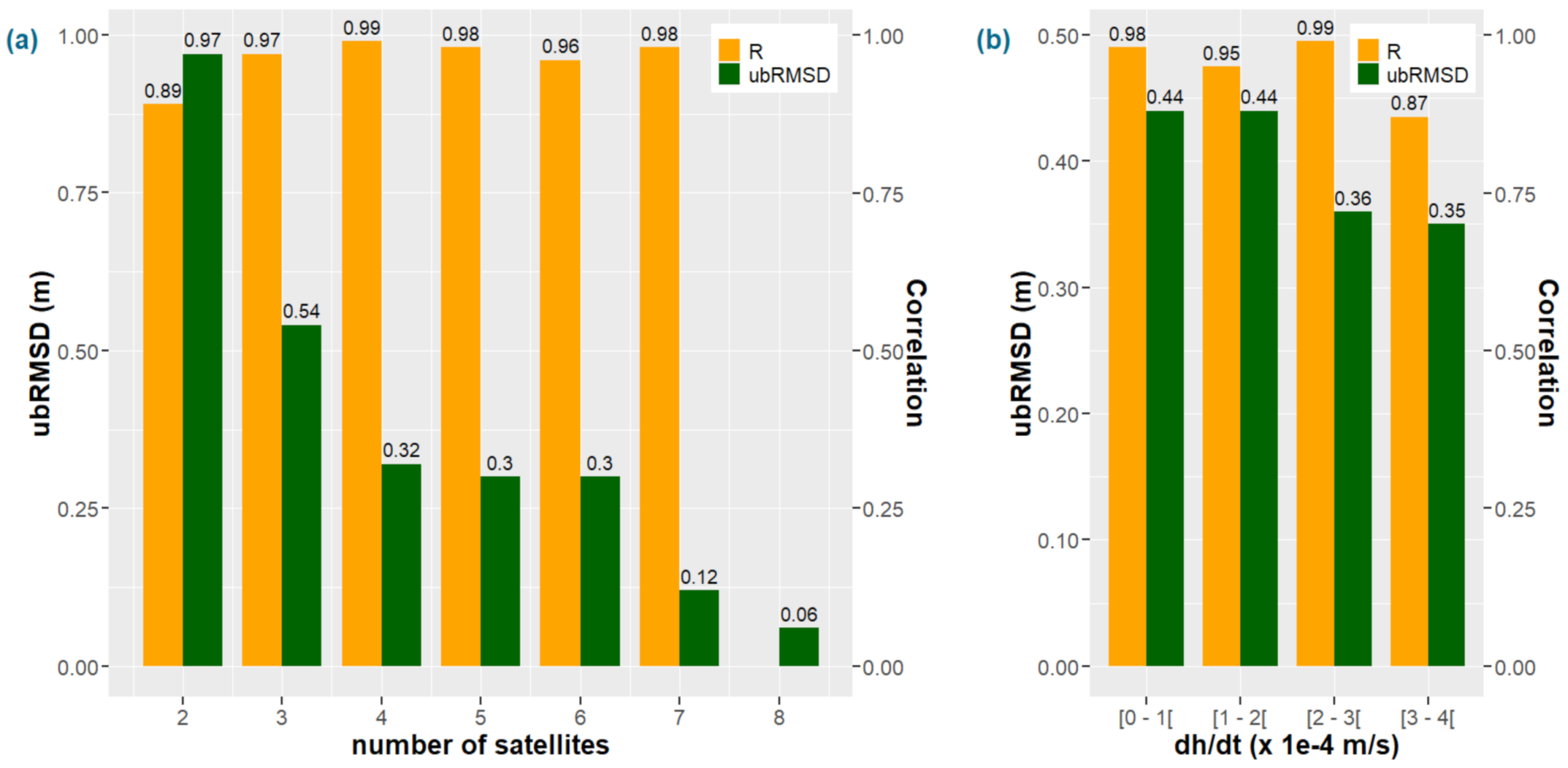
4.3. Influence of the Number of Satellites and Elevation Rate in the LSE Inversion

The number of GNSS satellites used to solve the system of equations with LSE ($n_{sat}$) appears to be a key point for the quality of the height retrieval. Following Equation (4), $\dot{h}$ also impacted the estimated frequencies and heights, as high $\dot{h}$ limits the application of static SNR retrieval methods [23]. In Figure 5c, the number of GPS ($n_{gps}$) and GLONASS ($n_{glo}$) satellites used for height inversion through the windowing of the dominant frequencies is presented. In Figure 5b, the vertical velocities $\dot{h}$ jointly estimated with h using LSE are shown.

Figure 5 is not sufficient to help us in separating the effects of $\dot{h}$ and $n_{sat}$ on height retrieval. The best qualitative results for all bands configurations were obtained from 2:30 p.m. to 4:30 p.m., and after 11:00 p.m. This corresponds to both relatively low vertical velocities ($\dot{h}<2\times {10}^{-4} \mathrm{m}·{\mathrm{s}}^{-1}$) and high number of satellites: $n_{sat}=n_{gps}+n_{glo}\ge 4$. On the contrary, the worst results were obtained from 5:30 p.m. to 7:00 p.m., and correspond to high $\dot{h}$ combined with a poor satellites configuration. Due to the study area characteristics (see Section 2.1), the number of satellites visible was frequently lower than three, and $\dot{h}$ reached $4\times {10}^{-4} \mathrm{m}·{\mathrm{s}}^{-1}$. It was then necessary to dissociate both influences by studying each separately.

Figure 6 shows the R and ubRMSD values as a function either of the number of satellites ($n_{sat}$, Figure 6a) or the vertical velocity of the reflecting surface ($\dot{h},$ Figure 6b) in the case of a L1 + L2 + L5 combined SNR inversion. The deterioration of the height retrieval was clear for $n_{sat}<4$. For $n_{sat}=2$ and $n_{sat}=3$, the correlations were 0.89 and 0.97 respectively, and the ubRMSD values were 0.97 m and 0.54 m. For $n_{sat}\ge 4$, the statistical results were homogeneous with R ≥ 0.96 and ubRMSD ≤ 0.32 m. We also notice that ubRMSD values fall to 0.12 m and 0.06 m respectively when $n_{sat}$ is equivalent to 7 and 8 (on a very small sample). Following the same methodology, we calculated maximum errors of 0.39 m and 0.14 m for $n_{sat}=7$ and $n_{sat}=8$ respectively. Although the maximum errors values listed in Table 1 are high, a very coherent result was observed when a sufficient number of satellites was observed to ensure the stability of the solution. The major influence of the number of satellites in the dynamic SNR height retrieval was assessed. On the contrary, the variations of $\dot{h}$ from ~0 to $4\times {10}^{-4}\mathrm{m}·{\mathrm{s}}^{-1}$ did not affect indisputably the quality of the height retrieval. For every $\dot{h}$ class extracted, ubRMSD values ranged from 0.35 m to 0.44 m and R from 0.87 to 0.99. A lower correlation was found for high $\dot{h}$ but ubRMSD was good, and the sample size is small. We conclude that using the dynamic SNR method, the influence of $\dot{h}$ (in the studied range) on the results was low.

5. Discussion

5.1. Retrieving Water Heights in Rivers with GNSS-R

When compared to previous studies on GNSS-IR SL or water height retrieval, our work distinguishes itself by the complexity of the study area: constraining azimuthal masks, narrow river, vegetation and complex phenomena affecting the river surface. This led to two main difficulties. First, a fewer number of available satellite tracks than for SL studies, which employ only elevations lower than 15° [22], or use a receiver installed on top of a lighthouse for dynamic SNR inversion [29], with a near-360° azimuthal range and a multielevation analysis. Second, a deterioration of the quality of frequency analysis with LSP highly affected by noise, leading to wrong estimations of the heights whatever the retrieval algorithm.

The visibility of the maximal number of satellites is a key point for all GNSS-IR height retrievals, and is limited for all-case studies on the rivers. Ideally, the receiver should be installed in a meander with land on the north, to maximize the azimuthal range with reflections on the river. The configuration in Podensac is not ideal for GNSS-R acquisition regarding this criterion: the Garonne River forms a straight line and the platform on which the GNSS antenna is installed is on the southwest riverbank. On the other hand, the shape of the river makes it a perfect case study for the spatial structure of tidal bores [26,27,31] by conventional means including the pressure sensor that was used as a reference. Anyway, while working on rivers a reduction of the number of available satellite tracks is inevitable.

The second point, with much noise in the raw LSP frequency output (Figure 4a), may be considered as the particularity of the Podensac site. First, the occurrence of tidal bores during spring tides introduces high-frequency perturbations unrelated to the water height in the SNR time series and had to be removed from the analysis. Then, the narrow width of the river combined with the presence of vegetation on the riverbanks masks the low-elevation tracks, which are the most adapted for altimetry [22]. With a river cross-section of about 180 m only, riverbanks plus trees up 30 m on the opposite side, potentially affect reflections up to a 10–15° elevation. Furthermore, a small sample of the low-elevation tracks may be affected by the vegetation as a secondary reflecting surface, and low-frequency perturbations are then introduced in the signal. This affects only one or all GNSS bands, as L1 can slightly penetrate the canopy deeper due to the wavelength difference between L2 and L5.

5.2. Influence of the GNSS Band, the Number of Satellites Visible and the Vertical Velocity

We computed SNR heights using multiple configurations of our adapted dynamic method (see the Results section). Characterizing the differences introduced by a change in several parameters, i.e., the GNSS bands used, the number of satellites visible, $n_{sat}$ and the vertical velocity $\dot{h}$, may lead to improvements in the quality of SNR-based height retrievals on rivers.

First, the use of the GNSS L1 or L2 band only did not show a specific deviation when compared to the multiband estimation (Figure 5a). Best results correlation ranged from 0.98 to 0.99 and ubRMSD ranged from 0.33 m to 0.31 m (Table 1). The single-band estimations contained some speckle noise in the output results, mainly due to a low number of distinct satellites visible, which was smoothed by the addition of L2 and L5 bands in the multifrequency analysis. Theoretically, the L2 P(Y) code is noisier and not appropriate for altimetry, while only GPS satellites from Block IIR-M (2005) and later blocks emit at L2C. Our results show that the noise in L2 SNR time series was removed from dominant frequency’s estimation, with consequently a lesser number of retrieved heights for L2 than for L1. The stability of the results was guaranteed whatever GNSS band combination we used: the bias between L1 and L2 estimations was 0.04 m.

When considering the maximum errors between SNR based heights and pressure water levels, we noticed that the values for a single band output (maximum error = 1.59 m for both L1 and L2) were lower than the value for the all-bands output. These values were high but if we look more in detail, they correspond to bad determinations when few satellites were visible, e.g., from 5:30 p.m. to 7:00 p.m. (see Figure 5a). At this time the L1 heights seemed correct but there was mostly no L2-only output due to poor satellite configuration and the filtering operations on noisy frequencies. We think that the addition of speckle L2 (and eventually L5) frequencies in the L1-only system of equations reduced, in this particular case, the stability of the solution. However, looking both qualitatively (see Figure 5a) and quantitatively (ubRMSD = 0.31 m), the solution with all GNSS bands performed slightly better on the entire time series. The combination of distinct GNSS frequencies reduced the variability of the output, especially when a sufficient number of distinct tracks was available. Moreover, when compared to the time series inverted with all GNSS bands, the L1-only and L2-only solutions contained 19.4% and 27.1% less determinations, respectively. We, therefore, recommend a multifrequency analysis, which should be combined with an increasing number of distinct tracks in the SNR data, to maximize the number of independent observations in height inversion. A perspective for further studies is the potential of the L5 band for altimetry [3]. The low amount of GPS/Galileo satellites equipped with L5 emitters in 2016 prevented us from retrieving a L5-only height estimation, but it would be interesting for further work.

Results depending on the elevation rate looked very stable. In Figure 6b, results were separated in four classes depending on the value of $\dot{h}$ ranging from 0 to $4\times {10}^{-4} \mathrm{m}·{\mathrm{s}}^{-1}$. Analyzing these small, subsampled time series, we observed that the deterioration of statistical indicators (R and ubRMSD) did not seem related to the increase of $\dot{h}$ value as expected. Correlations were great and ubRMSD ranged from 0.35 m to 0.44 m with lower values for high $\dot{h}$ during the rising tide. Our method offers the possibility to cover rapid events up to at least $5\times {10}^{-4} \mathrm{m}·{\mathrm{s}}^{-1}$ using GNSS-IR data.

With the major problem of GNSS-R retrievals on rivers being the azimuthal and elevation masks (see Section 5.1), a key point is the influence of the number of available tracks for SNR inversion ($n_{sat}$) on the final results. Figure 6a permits the analysis of statistical indicators for subsampled time series depending on $n_{sat}$, ranging from 2 to 8 in the Podensac case. Both R and ubRMSD showed an important deterioration for $n_{sat}$ < 4 and stable results in other cases: R ≥ 0.96 and ubRMSD ≤ 0.32 m for $n_{sat}$ ≥ 4. We also note that when $n_{sat}$ exceeded 6, the height comparison became excellent: ubRMSD = 0.12 m and maximum error = 0.39 m for $n_{sat}$ = 7, and ubRMSD = 0.06 and maximum error = 0.14 m for $n_{sat}$ = 8. Although definitive conclusions cannot be drawn due to the small sample size, this result looks very promising for further work with better environmental conditions. An increasing number of satellites systematically improved all the statistical indicators we used in this study.

We are optimistic about the potential of the SNR height inversion as a survey method for rapid water height evolution, in tides or flash floods as an example, for two reasons. First, in most cases, a receiver configuration with less constraining azimuthal and elevation masks can be installed to increase the number of satellites visible and the accuracy of heights inverted with the dynamic SNR method. Second, a true multiconstellations approach including Galileo and Beidou satellites (limited interest in 2016) could now be performed, including a L5-only height retrieval based on GPS and Galileo.

5.3. The Dynamic SNR Method

Following the specificities of the study area and the velocity of the rising tides, we chose to employ the dynamic SNR method (see Section 2.1 and Section 3.1). Would it be possible to retrieve equivalent or better results using a method that assumes a negligible $\dot{h}$ [23]? No dedicated study has been published, to our knowledge, on asymmetric phenomena with such a high amplitude as the tides in Podensac. Logical considerations make us think that these methods are not appropriate for a case study like Podensac. They are mostly employed on symmetric and predictable tides, and produce better results when amplitude is low [22]. The dominant frequencies are extracted with LSP, then heights are inverted assuming a quasi-static case ($\dot{h}<1\times {10}^{-6}\mathrm{m}·{\mathrm{s}}^{-1}$). Following this hypothesis only points in peaks and troughs of the tides can be correctly estimated. Various strategies help to reconstruct the complete time series: using tide models or functions (cubic splines) to fit the output SNR heights, and calculating a correction for the rate of change based on expected values. Furthermore, frequencies are extracted for each entire low-elevation subsampled satellite track, compromising the detection of rapid and unpredictable changes in the surface state with SNR time series.

On the contrary, the dynamic SNR method has arguments to deal with the problems enunciated above. First, the integration of the rate of change into a system of equations where h and $\dot{h}$ are jointly estimated with LSE being important: true values are directly extracted and no modelling or a priori knowledge of the phenomena is necessary. Second, the use of all-elevation SNR data (when not masked) as input, and the windowing of time series in the frequency estimations, produce finer detection of rapid changes in surface state. This is limited, as the influence of tidal bores, as an example, contaminated the results around 5:00 p.m. and had to be removed from the analysis (see Figure 4b,d and Figure 5a). However, this is an extreme case, being a highly nonlinear and extremely rapid ($\dot{h} ~ 1 \mathrm{m}·{\mathrm{s}}^{-1}$) phenomenon which occurs a few times a year. Third, the number of satellite tracks available can be a major issue while working on rivers, due to more constraining azimuthal and elevation masks, as in seas (see Section 4.3). The dynamic SNR method combines windowing with a multisatellite, multi-constellations and multi-frequency analysis, and provides good results with few satellites visible (Figure 5). This is of major interest as we look to extend the applications of GNSS-IR altimetry.

Following the idea in [25], we tried to add a new term to Equation (4) with the acceleration of the reflecting surface $\ddot{h}$. The LSE estimation then provides all h, $\dot{h}$ and $\ddot{h}$ values along with the dominant frequencies as inputs. The results for h and $\dot{h}$ looked like the without-acceleration case, with a small influence from acceleration. However, we noted an addition of speckle noise in the output h time series, so we finally rejected the idea. In [25], $\ddot{h}$ was calculated from true values or models. In our case, estimation was made from noisy frequencies based on the SNR time series (see Figure 4a). The derivative of h already adds noise in Equation (4). When deriving a second time for $\ddot{h}$ the noise level becomes prominent for a low gain, so including the acceleration has no advantage.

The noisy SNR time series in Podensac composed a challenging dataset. We were able to clean up the extracted dominant frequencies to retrieve h and $\dot{h}$ using two levels of filtering noise: first removal of the multipeaks in the LSP output that materialize other reflection surfaces or high frequency perturbations, then filtering of frequencies up to 3σ (99%) with an iterative approach of LSE. These additions to the initial method [29] were mandatory to work with GNSS-IR on very constraining river environments, of which Podensac is a perfect example.

A key last point is the sampling of output SNR height time series: the results presented in this study had a 1-min sampling period with the size of the moving window for the LSE of h and $\dot{h}$ being 5 min. The choice of a tiny window was made in opposition to the literature, where the lowest window size found was 2 h [25], applied to detect abrupt water-level changes in a reservoir with a 10-min sampling time series of heights. We thus showed that the use of the dynamic SNR approach provided a very high temporal resolution when compared to other methods. We could smooth the results over a longer time span but our thoughts are that this approach offers a distinct and complementary solution to other SNR retrieval algorithms, and can be used to extend the potential applications of GNSS-IR altimetry. Combining the high temporal resolution, its independence with any tide model or fitting function, and the ability to detect surface changes with high $\dot{h}$ (at least $5\times {10}^{-4} \mathrm{m}·{\mathrm{s}}^{-1}$), it opens the field to detection and monitoring of extreme events such as flash floods, marine surges in estuaries or coastal areas, tsunamis and storms.

6. Conclusions

In this study, SNR time series acquired over a narrow river were analyzed to retrieve the evolution of water height during asymmetric tides. The characteristics of the study area in Podensac made it a complicate environment for GNSS-R studies: the river shape forms a constraining azimuthal mask and disrupt low elevation signals, the tidal range is high (~6 m) and other high-frequency phenomena (i.e., tidal bores) affect the water surface and, thereby, the SNR time series during the acquisition.

The dynamic SNR method was chosen because it considers the dynamics of the reflecting surface during the height inversion [29], which is a key point for studying asymmetric and nonpredictable water level variations. The rising tide vertical velocity reached $5\times {10}^{-4} \mathrm{m}·{\mathrm{s}}^{-1}$, which is far more than the limit set for a static case ($1\times {10}^{-6} \mathrm{m}·{\mathrm{s}}^{-1}$ [23]). As the dominant frequencies estimated with LSP suffered noise, introduced in SNR time series by the river environment, we added a two-step filtering method to the dynamic inversion. First, the multipeaks were eliminated in the LSP output, then we iterated over the least square estimation (LSE) of h and $\dot{h}$ to remove the frequency values showing the greatest error when compared to estimation. This improved the results considerably when compared to the no-filtering inversion.

The best results obtained versus reference pressure water heights were consistent whatever the GNSS band we used: ubRMSD = 0.33 m for L1, ubRMSD = 0.32 m for L2, ubRMSD = 0.31 m for L1, L2 and L5 combined, with a correlation value higher than 0.98. The raw output without filtering the dominant frequencies showed ubRMSD = 1.56 m for L1. When combining all GNSS bands, a more robust estimation was found when enough satellites were visible; therefore it increased the number of samples in the output time series. Other factors are discussed including the influence of the vertical velocity of the reflecting surface and the number of distinct satellite tracks used in the LSE inversion. The influence of $\dot{h}$ on both R and ubRMSD values was low in the analyzed $0-5\times {10}^{-4} \mathrm{m}·{\mathrm{s}}^{-1}$ span. The dynamic SNR method fitted the reference data well, whatever the elevation rate of the reflecting surface. On the contrary, the number of tracks available had a major impact on the results. R and ubRMSD were consistent when $n_{sat}$ ≥ 4 with values greater than 0.96 and lower than 0.33 m, respectively. A clear degradation was observed for $n_{sat}$ = 2 (R = 0.89, ubRMSD = 0.97 m) or $n_{sat}$ = 3 (R = 0.97, ubRMSD = 0.54 m). Finally, we obtained a great result for a small subsample when $n_{sat}$ = 7 (ubRMSD = 0.12 m) and $n_{sat}$ = 8 (ubRMSD = 0.06 m). This latest point would have to be confirmed with longer time series analysis, but it is very promising for further work. Studies on rivers wider than the Garonne (~150 m), with more GNSS constellations (including Galileo, Beidou) and frequencies (recent developments of L5 band) would provide more available satellite tracks.

The windowing of the dynamic SNR method allows us to perform analyses with good temporal resolution when compared to previous methods. To take advantage of this point the sampling of our output time series of antenna heights is 1 min, and the size of the moving window is 5 min. The results exhibited good variations due to the rapid rising tide. It was also more subject to noise, because for tide modelling, at least a 2-h window is employed, which smooths the output time series. By contrast, this highlights the value of the dynamic SNR method to retrieve unpredictable water levels during extreme events with high elevation rates.

References

1. Bevis, M.; Businger, S.; Herring, T.A.; Rocken, C.; Anthes, R.A.; Ware, R.H. GPS Meteorology: Remote Sensing of Atmospheric Water Vapor Using the Global Positioning System. J. Geophys. Res. Atmos. 1992, 97, 15787–15801. [Google Scholar] [CrossRef]
2. Wickert, J.; Cardellach, E.; Martin-Neira, M.; Bandeiras, J.; Bertino, L.; Andersen, O.B.; Camps, A.; Catarino, N.; Chapron, B.; Fabra, F.; et al. GEROS-ISS: GNSS REflectometry, Radio Occultation, and Scatterometry Onboard the International Space Station. IEEE J. Sel. Top. Appl. Earth Obs. Remote Sens. 2016, 9, 4552–4581. [Google Scholar] [CrossRef] [Green Version]
3. Lestarquit, L.; Peyrezabes, M.; Darrozes, J.; Motte, E.; Roussel, N.; Wautelet, G.; Frappart, F.; Ramillien, G.; Biancale, R.; Zribi, M. Reflectometry With an Open-Source Software GNSS Receiver: Use Case With Carrier Phase Altimetry. IEEE J. Sel. Top. Appl. Earth Obs. Remote Sens. 2016, 9, 4843–4853. [Google Scholar] [CrossRef]
4. Hall, C.D.; Cordey, R.A. Multistatic Scatterometry. In Proceedings of the IEEE International Geoscience and Remote Sensing Symposium, Edinburgh, UK, 12–16 September 1988; pp. 561–562. [Google Scholar]
5. Martin-Neira, M. A Passive Reflectometry and Interferometry System (PARIS): Application to Ocean Altimetry. ESA J. 1993, 17, 331–335. [Google Scholar]
6. Kavak, A.; Vogel, W.J.; Xu, G. Using GPS to Measure Ground Complex Permittivity. Electron. Lett. 1998, 34, 254–255. [Google Scholar] [CrossRef]
7. Larson, K.M.; Small, E.E.; Gutmann, E.D.; Bilich, A.L.; Braun, J.J.; Zavorotny, V.U. Use of GPS Receivers as a Soil Moisture Network for Water Cycle Studies. Geophys. Res. Lett. 2008, 35, L24405. [Google Scholar] [CrossRef] [Green Version]
8. Rodriguez-Alvarez, N.; Camps, A.; Vall-Llossera, M.; Bosch-Lluis, X.; Monerris, A.; Ramos-Perez, I.; Valencia, E.; Martinez-Fernandez, J.; Baroncini-Turricchia, G.; Perez-Gutierrez, C.; et al. Land Geophysical Parameters Retrieval Using the Interference Pattern GNSS-R Technique. IEEE Trans. Geosci. Remote Sens. 2011, 49, 71–84. [Google Scholar] [CrossRef]
9. Chew, C.C.; Small, E.E.; Larson, K.M.; Zavorotny, V.U. Effects of Near-Surface Soil Moisture on GPS SNR Data: Development of a Retrieval Algorithm for Soil Moisture. IEEE Trans. Geosci. Remote Sens. 2014, 52, 537–543. [Google Scholar] [CrossRef]
10. Roussel, N.; Frappart, F.; Ramillien, G.; Darrozes, J.; Baup, F.; Lestarquit, L.; Ha, M.C. Detection of Soil Moisture Variations Using GPS and GLONASS SNR Data for Elevation Angles Ranging from 2° to 70°. IEEE J. Sel. Top. Appl. Earth Obs. Remote Sens. 2016, 9, 4781–4794. [Google Scholar] [CrossRef]
11. Zhang, S.; Calvet, J.C.; Darrozes, J.; Roussel, N.; Frappart, F.; Bouhours, G. Deriving Surface Soil Moisture from Reflected GNSS Signal Observations from a Grassland Site in Southwestern France. Hydrol. Earth Syst. Sci. 2018, 22, 1931–1946. [Google Scholar] [CrossRef] [Green Version]
12. Larson, K.M.; Gutmann, E.D.; Zavorotny, V.U.; Braun, J.J.; Williams, M.W.; Nievinski, F.G. Can We Measure Snow Depth with GPS Receivers? Geophys. Res. Lett. 2009, 36, L17502. [Google Scholar] [CrossRef] [Green Version]
13. Rodriguez-Alvarez, N.; Aguasca, A.; Valencia, E.; Bosch-Lluis, X.; Camps, A.; Ramos-Perez, I.; Park, H.; Vall-llossera, M. Snow Thickness Monitoring Using GNSS Measurements. IEEE Geosci. Remote Sens. Lett. 2012, 9, 1109–1113. [Google Scholar] [CrossRef]
14. Small, E.E.; Larson, K.M.; Braun, J.J. Sensing Vegetation Growth with Reflected GPS Signals. Geophys. Res. Lett. 2010, 37, L12401. [Google Scholar] [CrossRef]
15. Zhang, S.; Roussel, N.; Boniface, K.; Cuong Ha, M.; Frappart, F.; Darrozes, J.; Baup, F.; Calvet, J.C. Use of Reflected GNSS SNR Data to Retrieve Either Soil Moisture or Vegetation Height from a Wheat Crop. Hydrol. Earth Syst. Sci. 2017, 21, 4767–4784. [Google Scholar] [CrossRef] [Green Version]
16. Anderson, K.D. Determination of Water Level and Tides Using Interferometric Observations of GPS Signals. J. Atmos. Ocean. Technol. 2000, 17, 1118–1127. [Google Scholar] [CrossRef]
17. Larson, K.M.; Ray, R.D.; Nievinski, F.G.; Freymueller, J.T. The Accidental Tide Gauge: A GPS Reflection Case Study From Kachemak Bay, Alaska. IEEE Geosci. Remote Sens. Lett. 2013, 10, 1200–1204. [Google Scholar] [CrossRef] [Green Version]
18. Löfgren, J.S.; Haas, R. Sea Level Measurements Using Multi-Frequency GPS and GLONASS Observations. EURASIP J. Adv. Signal Process. 2014, 2014, 50. [Google Scholar] [CrossRef] [Green Version]
19. Vu, P.L.; Ha, M.C.; Frappart, F.; Darrozes, J.; Ramillien, G.; Dufrechou, G.; Gegout, P.; Morichon, D.; Bonneton, P. Identifying 2010 Xynthia Storm Signature in GNSS-R-Based Tide Records. Remote Sens. 2019, 11, 782. [Google Scholar] [CrossRef] [Green Version]
20. Purnell, D.; Gomez, N.; Chan, N.H.; Strandberg, J.; Holland, D.M.; Hobiger, T. Quantifying the Uncertainty in Ground-Based GNSS-Reflectometry Sea Level Measurements. IEEE J. Sel. Top. Appl. Earth Obs. Remote Sens. 2020, 13, 4419–4428. [Google Scholar] [CrossRef]
21. Tabibi, S.; Geremia-Nievinski, F.; Francis, O.; van Dam, T. Tidal Analysis of GNSS Reflectometry Applied for Coastal Sea Level Sensing in Antarctica and Greenland. Remote Sens. Environ. 2020, 248, 111959. [Google Scholar] [CrossRef]
22. Geremia-Nievinski, F.; Hobiger, T.; Haas, R.; Liu, W.; Strandberg, J.; Tabibi, S.; Vey, S.; Wickert, J.; Williams, S. SNR-Based GNSS Reflectometry for Coastal Sea-Level Altimetry: Results from the First IAG Inter-Comparison Campaign. J. Geod. 2020, 94, 70. [Google Scholar] [CrossRef]
23. Larson, K.M.; Löfgren, J.S.; Haas, R. Coastal Sea Level Measurements Using a Single Geodetic GPS Receiver. Adv. Space Res. 2013, 51, 1301–1310. [Google Scholar] [CrossRef] [Green Version]
24. Beckheinrich, J.; Hirrle, A.; Schon, S.; Beyerle, G.; Semmling, M.; Wickert, J. Water Level Monitoring of the Mekong Delta Using GNSS Reflectometry Technique. In Proceedings of the 2014 IEEE Geoscience and Remote Sensing Symposium, Quebec City, QC, Canada, 13–18 July 2014; pp. 3798–3801. [Google Scholar]
25. Tabibi, S.; Francis, O. Can GNSS-R Detect Abrupt Water Level Changes? Remote Sens. 2020, 12, 3614. [Google Scholar] [CrossRef]
26. Bonneton, P.; Bonneton, N.; Parisot, J.-P.; Castelle, B. Tidal Bore Dynamics in Funnel-Shaped Estuaries. J. Geophys. Res. Ocean. 2015, 120, 923–941. [Google Scholar] [CrossRef]
27. Martins, K.; Bonneton, P.; Frappart, F.; Detandt, G.; Bonneton, N.; Blenkinsopp, C.E. High Frequency Field Measurements of an Undular Bore Using a 2D LiDAR Scanner. Remote Sens. 2017, 9, 462. [Google Scholar] [CrossRef] [Green Version]
28. Frappart, F.; Roussel, N.; Darrozes, J.; Bonneton, P.; Bonneton, N.; Detandt, G.; Perosanz, F.; Loyer, S. High Rate GNSS Measurements for Detecting Non-Hydrostatic Surface Wave. Application to Tidal Borein the Garonne River. Eur. J. Remote Sens. 2016, 49, 917–932. [Google Scholar] [CrossRef] [Green Version]
29. Roussel, N.; Ramillien, G.; Frappart, F.; Darrozes, J.; Gay, A.; Biancale, R.; Striebig, N.; Hanquiez, V.; Bertin, X.; Allain, D. Sea Level Monitoring and Sea State Estimate Using a Single Geodetic Receiver. Remote Sens. Environ. 2015, 171, 261–277. [Google Scholar] [CrossRef]
30. Vu, P.-L.; Frappart, F.; Darrozes, J.; Ha, M.-C.; Dinh, T.-B.-H.; Ramillien, G. Comparison of Water Level Changes in the Mekong River Using Gnss Reflectometry, Satellite Altimetry and in-Situ Tide/River Gauges. In Proceedings of the IGARSS 2018—2018 IEEE International Geoscience and Remote Sensing Symposium, Valencia, Spain, 22–27 July 2018; pp. 8408–8411. [Google Scholar]
31. Bonneton, P.; Filippini, A.G.; Arpaia, L.; Bonneton, N.; Ricchiuto, M. Conditions for Tidal Bore Formation in Convergent Alluvial Estuaries. Estuar. Coast. Shelf Sci. 2016, 172, 121–127. [Google Scholar] [CrossRef]
32. Bishop, G.J.; Klobuchar, J.A.; Doherty, P.H. Multipath Effects on the Determination of Absolute Ionospheric Time Delay from GPS Signals. Radio Sci. 1985, 20, 388–396. [Google Scholar] [CrossRef]
33. Strandberg, J.; Hobiger, T.; Haas, R. Improving GNSS-R Sea Level Determination through Inverse Modeling of SNR Data: GNSS-R INVERSE MODELING. Radio Sci. 2016, 51, 1286–1296. [Google Scholar] [CrossRef] [Green Version]
34. Santamaría-Gómez, A.; Watson, C.; Gravelle, M.; King, M.; Wöppelmann, G. Levelling Co-Located GNSS and Tide Gauge Stations Using GNSS Reflectometry. J. Geod. 2015, 89, 241–258. [Google Scholar] [CrossRef]
Figure 1. Location of the study area. (a) Location of Podensac on the Garonne River; (b) the Gironde/Garonne/Dordogne estuary in southwest France; (c) drone image of the Garonne River taken by V. Marie (EPOC), showing the first waves of the tidal bore, its direction of propagation, and the platform location; (d) photo of the Garonne River from the platform with the GNSS antenna installed. The narrowness of the river and the vegetation on riverbanks are visible in both images.
Remotesensing 13 01856 g001
Figure 2. 1-Hz resampled pressure water level time series of the Garonne River at Podensac. (a) During the GNSS-R SNR acquisition with red rectangle indicating tidal bores; (b) during four consecutive tide periods. These figures are representative of the entire pressure water level time series and do not show the tidal oscillations over a longer period, as the acquisition was performed during spring tides only when both the tidal range is maximum and tidal bores can form.
Remotesensing 13 01856 g002
Figure 3. Flowchart of the dynamic SNR method with our improvements adapted from [29]. (a) Processing chain with the addition of a two-step filtering of the dominant frequencies (in orange); (b,c) respective examples of a single-peak output and a multipeak output from LSP for the same satellite track (G01). Red line materializes the level of filtering which depends on parameter k (here k = 0.6), and f ˜ ~100 Hz.
Remotesensing 13 01856 g003
Figure 4. Dominant frequencies extracted from GPS (green) and GLONASS (orange) satellites using the LSP, and river heights inverted with the dynamic SNR method (blue) compared to pressure water levels (red). (a,b)   f ˜ and h from raw LSP output respectively; (c) frequencies filtered out after multipeak rejection with parameter k = 0.6 and iterative LSE; (d) concordant time series of water levels estimated with iterative LSE. Grey areas are masks due to tidal bore occurrence (17 h) and data gaps (21–22 h).
Remotesensing 13 01856 g004
Figure 5. Final results using the adapted dynamic SNR inversion. (a) Comparison of h calculated using L1 only (orange), L2 only (green), and L1 + L2 + L5 (blue) frequencies for GPS and GLONASS satellites with pressure water levels (red); (b) output h ˙ with L1 + L2 + L5 bands; (c) number of GPS and GLONASS satellites for the calculation of h and h ˙ . The value of h ˙ was derived from the relative antenna height h, thus it was negative during rising tides as the relative antenna height decreased.
Remotesensing 13 01856 g005
Figure 6. Statistical results depending on the number of satellites and the vertical velocity. (a) R and ubRMSD computed according to the number of satellites for the inversion of h and h ˙ ; (b) Idem according to the vertical velocity class (intervals computed with range 1 × 10⁻⁴ m.s−1).
Remotesensing 13 01856 g006