Optical Remote Sensing Image Denoising and Super-Resolution Reconstructing Using Optimized Generative Network in Wavelet Transform Domain

Abstract

High spatial quality (HQ) optical remote sensing images are very useful for target detection, target recognition and image classification. Due to the influence of imaging equipment accuracy and atmospheric environment, HQ images are difficult to acquire, while low spatial quality (LQ) remote sensing images are very easy to acquire. Hence, denoising and super-resolution (SR) reconstruction technology are the most important solutions to improve the quality of remote sensing images very effectively, which can lower the cost as much as possible. Most existing methods usually only employ denoising or SR technology to obtain HQ images. However, due to the complex structure and the large noise of remote sensing images, the quality of the remote sensing image obtained only by denoising method or SR method cannot meet the actual needs. To address these problems, a method of reconstructing HQ remote sensing images based on Generative Adversarial Network (GAN) named “Restoration Generative Adversarial Network with ResNet and DenseNet” (RRDGAN) is proposed, which can acquire better quality images by incorporating denoising and SR into a unified framework. The generative network is implemented by fusing Residual Neural Network (ResNet) and Dense Convolutional Network (DenseNet) in order to consider denoising and SR problems at the same time. Then, total variation (TV) regularization is used to furthermore enhance the edge details, and the idea of Relativistic GAN is explored to make the whole network converge better. Our RRDGAN is implemented in wavelet transform (WT) domain, since different frequency parts could be handled separately in the wavelet domain. The experimental results on three different remote sensing datasets shows the feasibility of our proposed method in acquiring remote sensing images.

1. Introduction

High spatial quality (HQ) optical remote sensing images have the characteristics of high spatial resolution (HR) and low noise, which can be widely used in agricultural and forestry monitoring, urban planning, military reconnaissance and other fields. However, the time and cost of development and the vulnerability of the image to changes in atmosphere and light are the reasons for the acquisition of a large number of low spatial quality (LQ) remote sensing images. So, how to obtain HQ images economically and conveniently has been a major challenge in the field of remote sensing.

Recently, more researchers have paid attention to recovering HQ remote sensing images from LQ ones using image processing technology.

Low spatial resolution (LR) and noise are two common factors causing low quality of remote sensing images [1]. So, enhancing spatial resolution and denoising are two of the most common approaches to acquire high quality images.

Generally, image SR reconstruction and denoising methods mean adding useful information (HR details) to LQ images and removing useless information (noise) from LQ images, respectively. Due to the existence of multiple solutions for any pixel in a LR image, SR methods are ill-posed problems [2]. Basically, SR methods include Single Image Super-Resolution (SISR) and Multi-Image Super-Resolution (MISR) according to the number of LR image, because, in the field of remote sensing research, image data are not abundant. However, the MISR method obtains HR images by processing a set of LR images which have only slightly different views, so the SISR method is commonly used in the remote sensing field, which acquires a HR image through a single LR image. Interpolation-based [3,4], reconstructed-based [5,6] and example-based [7] are three common classifications of SISR methods. This article does not discuss interpolation-based methods and reconstructed-based methods since these two types of methods are usually treated as traditional methods. For example, moments-based methods are very popular in image reconstruction [8,9,10,11]. Example-based methods establish the relationship between LR and HR images to reconstruct the high-frequency part of the LR images. In recent years, with the development of big data technology, machine learning methods have become increasingly popular and practical. Deep learning methods, which usually mean deep convolutional neural networks (CNN) [12,13,14], are currently one of the research hot-spots. Deep learning methods have achieved impressive results in many fields such as image processing. In particular, the SR algorithm based on deep learning has achieved significantly better results than the traditional SR reconstruction algorithm [15,16,17,18,19]. This algorithm has also achieved excellent results in the field of SR reconstruction of remote sensing images [7,20,21]. SRCNN, which is the first SR method based on CNN, was proposed by Dong et al. [2,22]. SRCNN borrows the idea of parse-coding SR method. However, if SRCNN deepens the number of layers, it will become very difficult to train. Then, with the emergence of residual learning techniques, deeper networks could be designed to achieve better results. The VDSR published by Kim et al. [23] is the earliest and most typical method of using residual learning. Recently, Generative Adversarial Network (GAN) based methods are getting popular because these methods could generate more interesting results. SRGAN [24] is the first GAN-based SR method that could reconstruct more details than the normal non-GAN-based method. After that, ESRGAN [25] is proposed, which is the enhancement of SRGAN, and this method achieved the state-of-the-art effect that time.

The problems of image denoising and SR are similar because both of them mainly process the parts of high-frequency, but keep other information preserved. Model-driven traditional maximum posteriori and data-driven modern deep learning method are two categories of image denoising algorithm. The model-driven approach accomplishes the task of denoising by constructing a reasonable maximum posteriori model. The biggest disadvantage of the model-driven approach is that it relies too much on the assumption of image priori and noise distribution given in advance. When the assumption deviates from the real situation of the actual data, the established model is no longer applicable. Recently, the data-driven method has achieved good results in image denoising. Its operation mode is: using pairs of noised image and corresponding clean image as inputs and outputs to train a pre-designed deep network with an end-to-end approach. The well-trained architecture could be directly regarded as a function, which could use the noised image as input to acquire the corresponding restored image.

The above methods have achieved some results, but there is still room for improvement. First, Most of the existing methods mentioned above only employ denoising or SR technology to obtain HQ optical images. However, due to the complex structure [1] and the large noise of remote sensing optical images, the quality of image obtained only by denoising method or SR method cannot meet the actual needs. So, how to handle the two problems fast and accurate is very important and meaningful for acquiring HQ optical remote sensing images. Second, non-GAN-based methods could achieve better Peak Signal-to-Noise Ratio (PSNR) results, but details in these results are more blurry than the results that GAN-based methods achieved. However, GAN-based methods are difficult to train because when the discriminator is well trained, the generator gradient disappears and the loss cannot be lowered. When the discriminator is poorly trained, the generator gradient is inaccurate. Only if the discriminator is not well trained can it be good. However, it is difficult to grasp this fire. Even in different stages before and after the same round of training, this fire may be different, so GAN-based methods are so difficult to train. Third, most of methods mentioned above only handle image denoising or SR problems in spatial domain directly, which we think is not suitable because different high frequencies corresponding different detailed information should be processed differently, which cannot be distinguished well in the spatial domain. To address the above-mentioned problems, an end-to-end CNN-based method named “Restoration Generative Adversarial Network with ResNet and DenseNet” (RRDGAN) that could handle the two problems using one network in the meantime is proposed by us. Considering that residual learning could reuse features implicitly and the dense connection keeps exploring new features, we combine the benefit of the three network structure as our generator to achieve a better effect. We furthermore use total variation (TV) loss [26] to achieve better edge details since Rudin et al. [27] observed that the TV of noise-polluted images was significantly greater than that of noise-free images. Then, we use the idea of Relativistic GAN [28] to optimize our discriminator to make the whole network converge better. Not only that, considering most of the remote sensing image denoising and SR methods are carried out directly in the spatial domain and processing different frequency parts of a remote sensing image is the key step to both denoising and SR reconstruction, so to furthermore improve the performance of our methods, RRDGAN is implemented in WT domain instead of directly in spatial domain. So, Figure 1 illustrates the result of improving the quality of remote sensing images (4 times SR with 25 level Gaussian noise removal) in spatial domain or in WT domain, respectively. We could see that the result in WT domain is obviously better than in spatial domain.

In conclusion, The following three aspects are the contribution of this article:

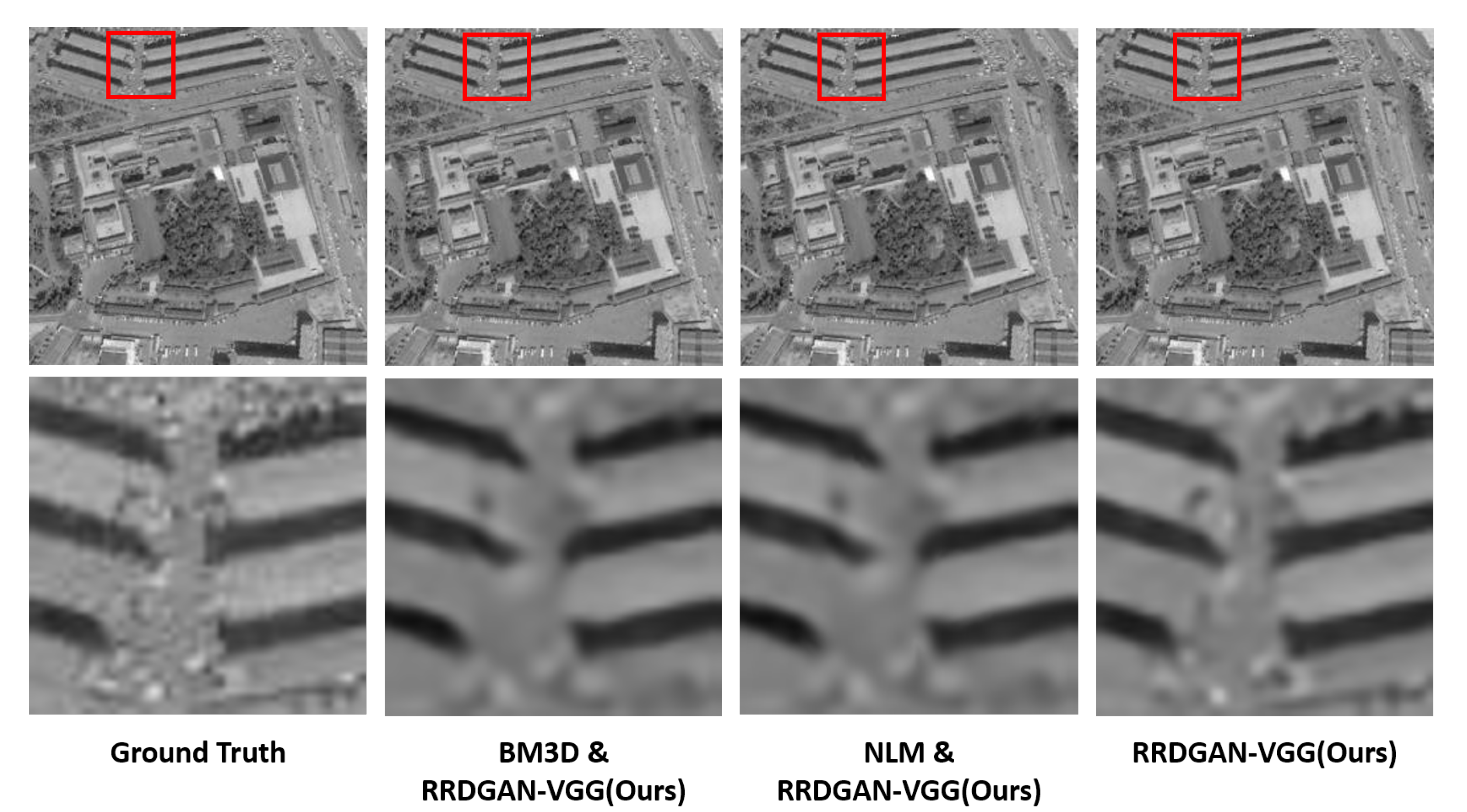
• A method named RRDGAN is proposed. RRDGAN combines denoising and super-resolution reconstruction into a unified framework to obtain better quality optical remote sensing images.
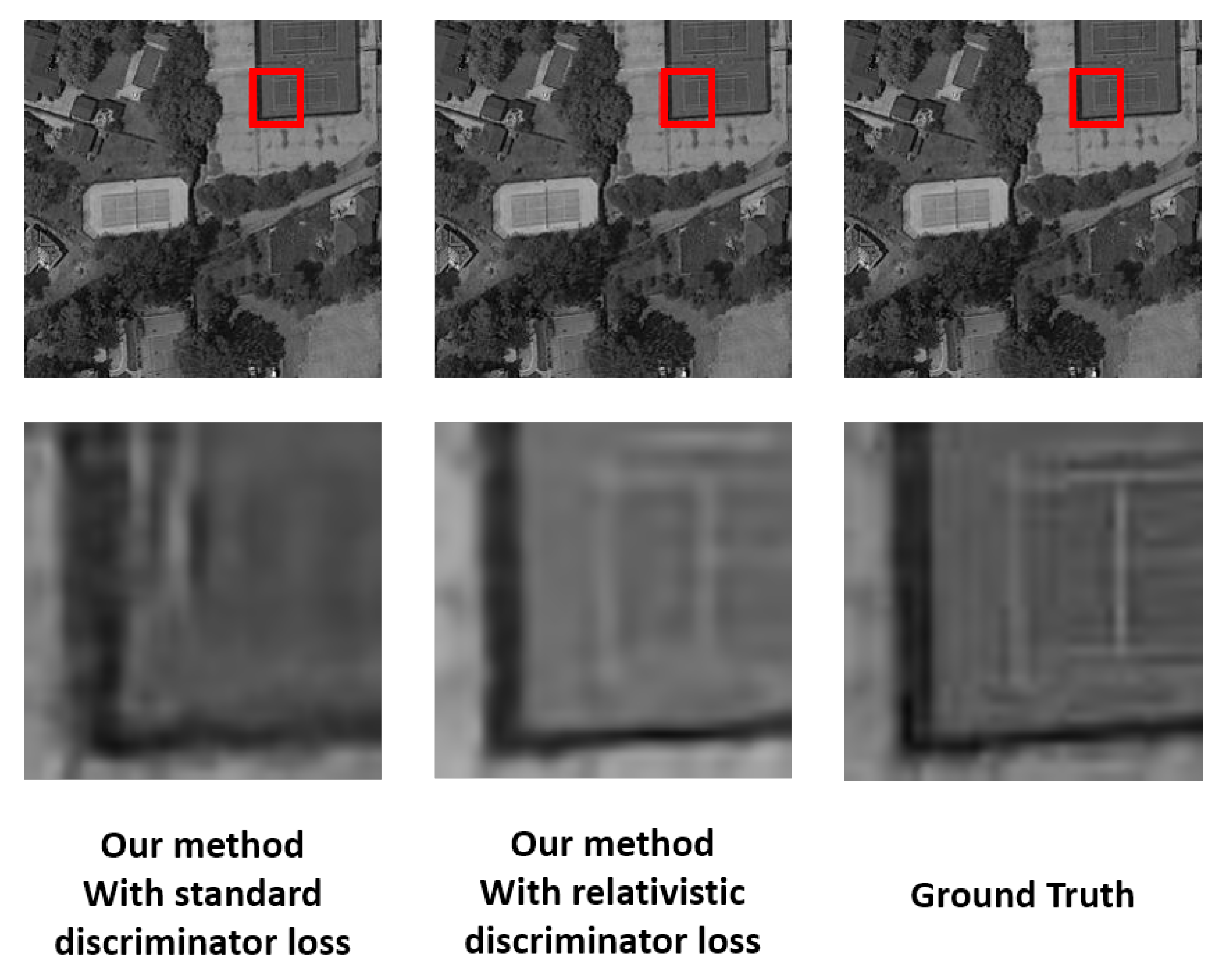
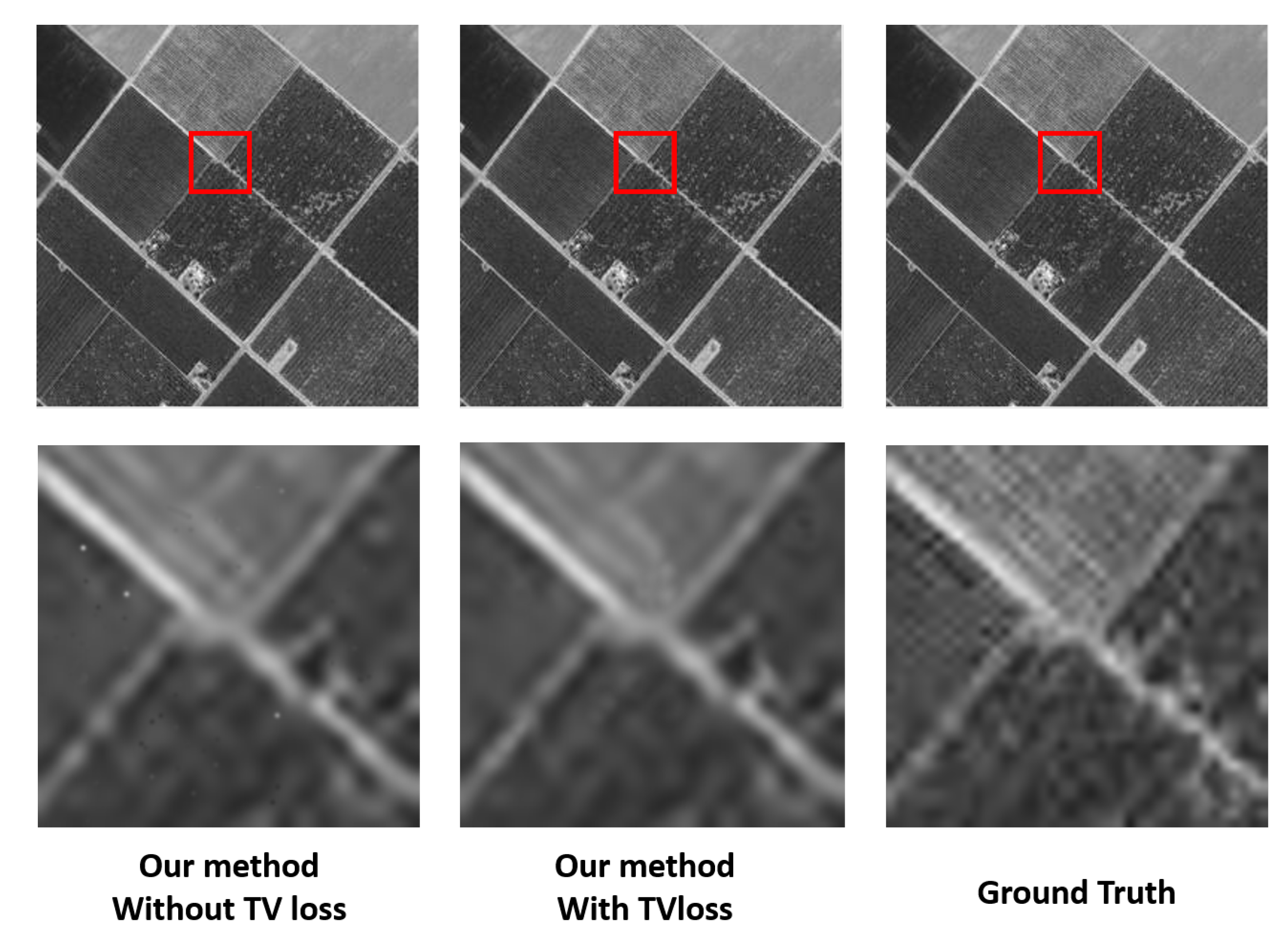
• The generator of RRDGAN combines residual learning and dense connection to obtain better PSNR results, and the discriminator uses relativistic loss to make the entire network converge better. Generator also uses TV loss to reconstruct better details.
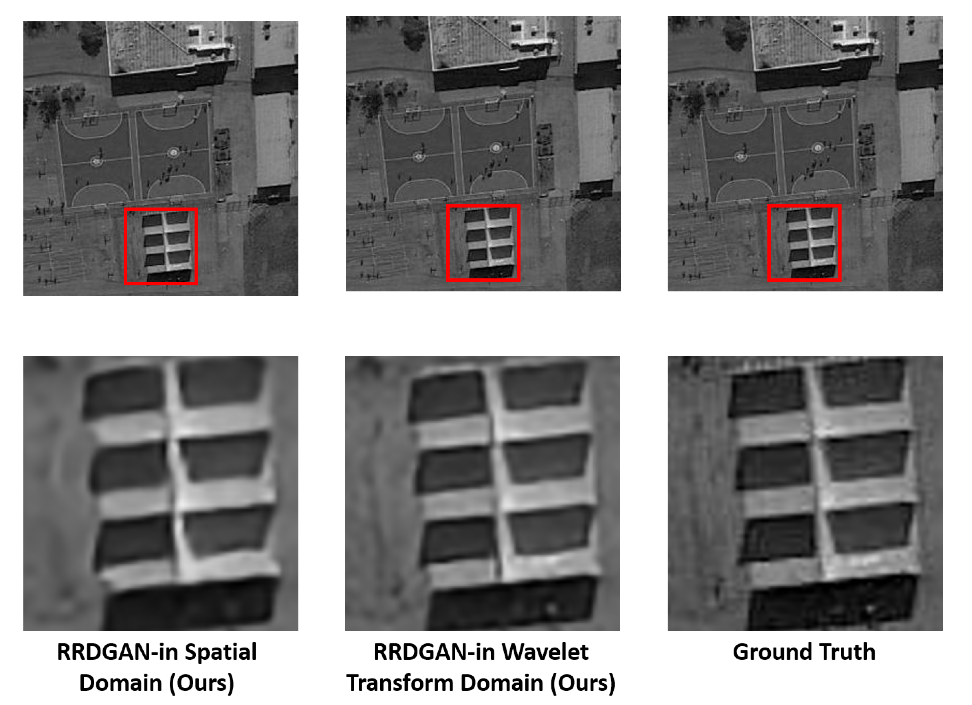
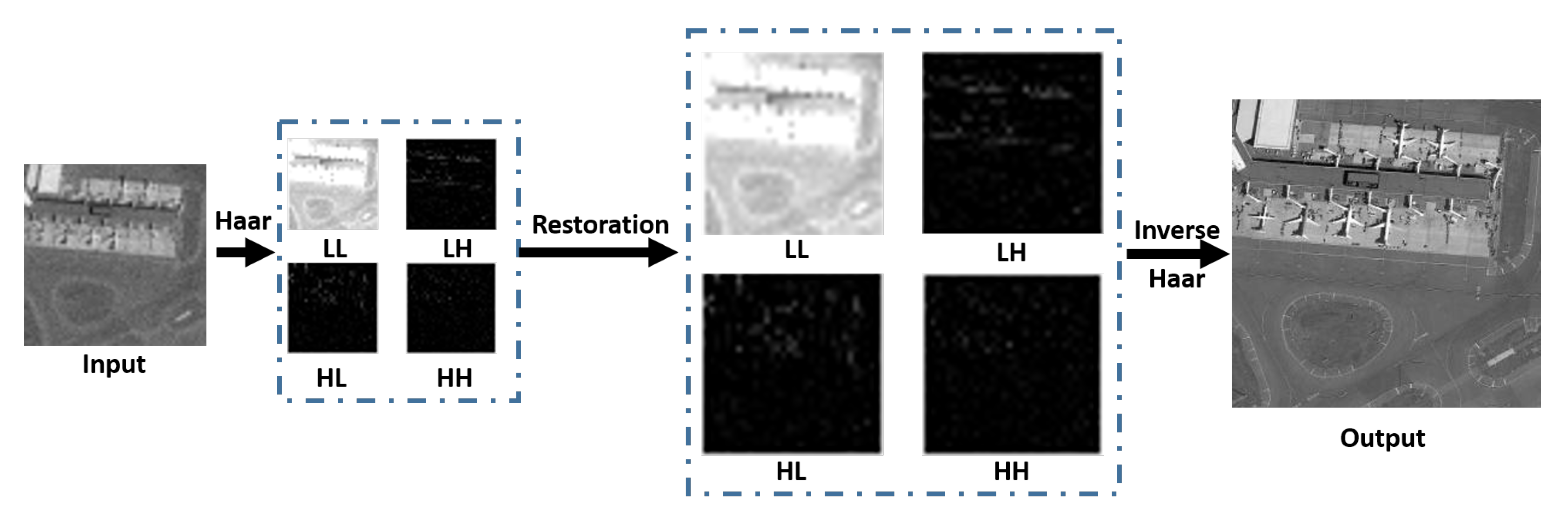
• RRDGAN is implemented in WT domain, which could handle different parts of LR image well, respectively.

The rest of this article is organized as follows. Section 2 introduces related works in handling single image denoising and SR reconstruction methods. Section 2 also recommends the related works about processing these problems in WT domain. Section 3 gives the implementation details of our RRDGAN. Section 4 describes the experimental results. Section 5 gives some discussions about this article and conclusion is drawn in Section 6.

2. Related Works

2.1. Optical Image Super-Resolution Reconstruction Method

As mentioned above, the recent research hotspot in image processing is a CNN-based method because CNN could extract more exact image features gradually as the network layers get deeper, which could achieve better results than traditional methods and human eyes. As mentioned above, SRCNN, which is the first SR method using CNN, was proposed [2] in 2016. Then, various CNN-based SR methods keep coming out every year. Kim et al. [23] proposed the first SR method-based residual learning, which deepens the network to 20 layers. After that, Laplacian Pyramid SR CNN (LapSRN) was proposed by Lai et al. [29], and it could gradually reconstruct high-frequency details in different sub-bands of potential remote sensing images. Then, a SR method based on dense connection was proposed by Tong et al. [30], which made CNN layers deeper and became the state-of-the-art (SOTA) SR method that time.

Nowadays, GAN-based methods are getting more popular in image processing research areas. Different from those SR methods, who use PSNR to evaluate the effect, SRGAN, which is proposed by Ledig et al. [24], is the first GAN-based SR method. In addition to using PSNR, SRGAN uses Mean Opinion Score (MOS) [24] to evaluate the effect, which could evaluate human visual effect of an image. The generative part of this method, named Super-Resolution Residual Network (SRResnet) is a CNN structure, which combines local and global residual learning. The adversarial part of this method is a very ordinary CNN structure, which could discriminate whether an image is ground truth or the result of SR reconstruction. In this article, the authors compare the SR reconstruction result of some typical methods, including SRResnet. The comparison result shows that the PSNR result of SRGAN is not the highest among these SOTA methods. However, when using MOS to evaluate the reconstruction effect, we could see that SRGAN achieves the highest score in MOS, and we could also see that SRGAN reconstructs more details than other non-GAN methods do, even including SRResnet. This is because PSNR-based method uses MSE to compute the loss between reconstructed image and ground truth, which could make reconstructed images smoother. So, in general, PSNR is not the only rule to judge whether the reconstructed image is good or not.

2.2. Single Image Denoising Method

Similarly, CNN-based denoising methods are also popular recently. Jain et al. [31] proposed the first CNN-based denoising method. Compared with other traditional methods, this method achieves similar or even better results. DnCNN was proposed by Zhang et al. [32], which combines batch normalization with residual learning and obtained the latest results. Then, an automatic encoder with symmetric jump connection network was proposed by Mao et al. [33]. The method realizes 10 pairs of symmetric convolution and deconvolution layers, the first 5 layers are the coding layer, while the last 5 layers are the decoding layer. Therefore, the image denoising network based on CNN becomes more and more profound.

2.3. Single Image Restoration in Wavelet Transform Domain

Remote sensing image restoration methods in spatial domain usually handle high frequency and low frequency parts together, which is not very appropriate. We should pay more attention in processing different high frequency parts, especially high frequency part because SR problem and some typical noises (e.g., salt and pepper noise) are related to the high frequency part. So, a good way to deal with image restoration problems is treating different frequency parts separately. WT has been proven to be a very effective image restoration method [20,34]. An image could be transformed into a series of coefficients in the same size by WT operation. It is suitable to predict the wavelet coefficients by exploiting the sparse coding algorithm and reconstructing the HQ optical image for the detail of seed band, which is very sparse.

A typical Haar WT operation is showed in Figure 2. As illustrated in Figure 2, LL is the low frequency sub-band of the original image, which represents the global topology. The other three sub-bands (HL, LH and HH in the figure) represent the high frequency part in vertical, horizontal and diagonal orientations, respectively. By the way, using the inverse implementation of wavelet transformation, we could acquire the final image with these four sub-band coefficients.

A SR method using 3D-CNN in WT domain was proposed by Yang et al. [35]. This method first uses 3D-CNN to acquire features, then decomposes these features into wavelet coefficients. After that, these wavelet coefficients with 3D-CNN can be handled to get the reconstructed coefficients and finally, the reconstructed image would be obtained by inverse wavelet transform. This method requires multi-frame images to accomplish 3D-CNN, which is not convenient for the remote sensing research area.

3. Proposed Method

In this section, we give the problem definition first and then the details of our proposed method following.

3.1. Problem Definition

To achieve our ultimate goal, which is to reconstruct a HQ optical remote sensing image from a LQ one, the relationship between LQ remote sensing image and its HQ reconstructed result should be established. So, the purpose of our method is to process denoising and SR problems simultaneously by establishing a mapping F from LQ image to its HQ reconstructed counterpart through a CNN-based network. In this article, the LQ image is denoted as Y, and recovering Y from an image $F$(Y) is our goal. In this article, RRDGAN is the mapping F.

As illustrated in Figure 3, the generator of our method mainly includes four steps. First, Haar wavelet transformation is implemented to decompose the input LQ remote sensing image into four sub-band coefficients. Second, these coefficients would be sent into our generator, which is a deep network, to acquire the reconstructed sub-bands coefficients. Finally, the output image is acquired by Haar inverse wavelet transformation. To accomplish the adversarial part, both the reconstructed image and spatial ground truth would be sent into a typical CNN-base network, which is similar to the discriminator of SRGAN. After these steps, we will get a well-trained network, which could improve the spatial quality of remote sensing images.

3.2. Proposed Method

Our network architecture is introduced in this section. The proposed method RRDGAN is illustrated in Figure 4. The LQ images were obtained by downsampling the HQ optical images using bicubic kernel with factor r = 4, then adding some typical noises.

Compared with SRGAN, we made two modifications to achieve better performance on remote sensing images. First, we combined residual learning and dense connection to replace the original SRResnet, which is the generative part. Then, we used Realistic GAN loss function to train the discriminator part.

3.2.1. Network Architecture

The Discriminator aims to distinguish whether the estimated HQ optical images are plausible or not. Different from the original SRGAN, our discriminator is based on Relativistic GAN. The discriminator takes both the real reconstruction result and the fake reconstruction result as inputs. The recent Relativistic GAN [24] is one improvement of the original GAN which could distinguish a real sample and a fake one better. So, we apply Realistic GAN instead of the original GAN in our discriminator, which could further improve the performance.

The Generator processes remote sensing input images in wavelet transform domain. It first enlarges the input image twice by simply bicubic method, because applying Haar wavelet transform to the image will result in four sets of coefficients that are one-fourth the size of the original image. Then, it sends the four wavelet transform coefficients into a deep network, which combines the advantages of residual learning and densely connection, respectively, to restore the coefficients, which could be used to acquire final high quality images.

In our generator, residual learning and dense connection are the most important implementations. Residual learning is learning the residual between the input and output, so in this article, we define a residual $r=y-x$, most of which may be zero or less [14]. In this equation, r is the residual pixel of x and y. Dense connection is defined as $d=h\left(\left[x_0,x_1,...,x_l\right]\right)$, where $[x_0,x_1,\dots ,x_l]$ refers to the concatenation of feature-maps produced in layers $x_0,x_1,\dots ,x_l$ [13].

Residual learning and dense connection have a complex relationship. Residual learning could reuse features implicitly, but it is not good at exploring new features. In contrast, the dense connection keeps exploring new features, but suffers from higher redundancy [36]. So, we fuse these two structure and achieve both advantages. Each Dense-Residual-Block (DRB) contains a densely connection branch and a residual learning branch. The residual learning branch consists of one 1 × 1 filter, one 3 × 3 filter and one 1 × 1 filter. The densely connection branch concatenates the input and residual learning output. There are 20 DRB blocks in our generator part. The final upsampling implementation is inspired by ESPCN [37], which could upscale the last feature maps into the HR output by using an efficient sub-pixel convolution layer. What needs to be illustrated is that we remove all BN operations in our generator part for the reason of keeping BN operations that could not achieve better performance than removing them.

3.2.2. The Loss Function

The Discriminator uses idea of relativistic GAN, we define the discriminator loss as:

$$L_D=-{\mathbb{E}}_g\left[log\left(D(g,f)\right)\right]-{\mathbb{E}}_f\left[log\left(1-D(f,g)\right)\right]$$

(1)

In this equation, ${\mathbb{E}}_g\left[·\right]$ and ${\mathbb{E}}_f\left[·\right]$ represent the average of all the ground truth or reconstructed image in one mini-batch, respectively. D is defined as equation

$$D\left(g,f\right)=\sigma \left(O\left(g\right)-\mathbb{E}\left[O\left(f\right)\right]\right)$$

(2)

$$D\left(f,g\right)=\sigma \left(O\left(f\right)-\mathbb{E}\left[O\left(g\right)\right]\right)$$

(3)

In this equation, O, g and f represent the non-transformed discriminator output, the ground truth and reconstructed image by generator, respectively.

The Generator loss function includes three parts: content loss, adversarial loss and TV loss. Instead of MSE loss, VGG loss is chosen to be our content loss [24] in our generator, which is defined as:

$$L_{VGG}=\frac{{\sum }_{j=1}^{N_{i,j}}\left({\sum }_{i=1}^{M_{i,j}}{\left({\varphi }_{i,j}\left(F\left(Y\right)\right)-{\varphi }_{i,j}\left(X\right)\right)}^2\right)}{M_{i,j}{N}_{i,j}}$$

(4)

In this content loss equation, ${\varphi }_{i,j}$ is the feature map obtained by the j-th convolution of the well-trained VGG19 network before the i-th maxpooling layer. X is the HQ image, and $F\left(Y\right)$ is the reconstructed image. M is the row number of image X, and N is the column number of image $F\left(Y\right)$.

Furthermore, the adversarial loss is similar to discriminator loss:

$$L_G=-{\mathbb{E}}_g\left[log\left(1-D(g,f)\right)\right]-{\mathbb{E}}_f\left[log\left(D(f,g)\right)\right]$$

(5)

Finally, TV loss is defined as (6). in order to enhance the edge information of the reconstructed image. Rudin et al. [27] observed that the TV of noise-polluted images was significantly greater than that of noise-free images, so in image super-resolution and denoising, TV regularization is a structured restoration method aimed at preserving image details.

$$L_{TV}=\sum _{i,j}\sqrt{{\left|y_{i+1,j}-y_{i,j}\right|}^2+{\left|y_{i,j+1}-y_{i,j}\right|}^2}$$

(6)

As showed in (6), y represents the reconstructed image, and $i,j$ represent the pixel horizontal and vertical positions in the image, respectively.

In summary, the loss function for the generator is similar to SRGAN, which is illustrated as follows:

$$L_{G_{all}}=L_{VGG}+\lambda L_G+\beta L_{TV}$$

(7)

In this equation, $\lambda$ and $\beta$ are the coefficients to balance different loss terms.

4. Experimental Results

In this experimental results section, the datasets this article used are described first, then experimental results are illustrated.

4.1. DataSets

In our experiment, three datasets were used to verify the performance of RRDGAN. The three datasets are: UCMERCED [38], NWPU-RESISC45 [39] and GaoFen-1. Among these datasets, UCMERCED includes 21 land-use scene classes. All these classes have high spatial resolution (0.3 m/pixel). NWPU-RESISC45 is proposed by Northwestern Polytechnical University (NWPU). This dataset is a public benchmark and has 31,500 images in total. These images could be divided into 45 scenes. The size of each image in UCMERCED and NWPU-RESISC45 is 256 × 256 pixels. GaoFen-1 is the dataset of multispectral images which are obtained by GaoFen-1 satellite. We choose to mix these three datasets instead of implementing the three datasets, respectively. Then, 135 images are randomly chosen for training, while another 40 images are randomly chosen for testing.

4.2. Implementation Details

The LQ images (96 × 96) for training were acquired by downsampling the ground truth (256 × 256) with factor 4, then adding noise on them. As Figure 5 and Figure 6 show, two types of noise are added, respectively, in our experiments: White Gaussian noise with level 25, and salt and pepper noise with level 0.005. The total number of these LQ image/HQ image pairs is 135, which are from three datesets. These images belong to various types, including airplane, church, forest, wetland and so on.

Finally, we added a total of 20 DPN blocks. The learning rate is 0.0001 in the beginning, $\lambda$ in Equation (7) is ${10}^{-3}$ and decayed by a factor of 0.1 every ${10}^5$ iterators. The environments of implementing these experiments are Nvidia GTX 1080Ti, Inter Genuine Inter CPU 1.4 GHz, 64 GB RAM, and the tensorflow-1.14.0 package.

For the sake of fairness, VDSR, SRGAN and ESRGAN are well retrained using the datasets mentioned above.

By the way, the reason we choose to use Haar wavelet is that Haar wavelet is one of the simplest and fastest wavelet transform methods, and processing the four frequency sub-bands obtained by Haar wavelet can achieve the expected denoising and super-resolution reconstruction effect in this paper, and the processing speed is also satisfactory.

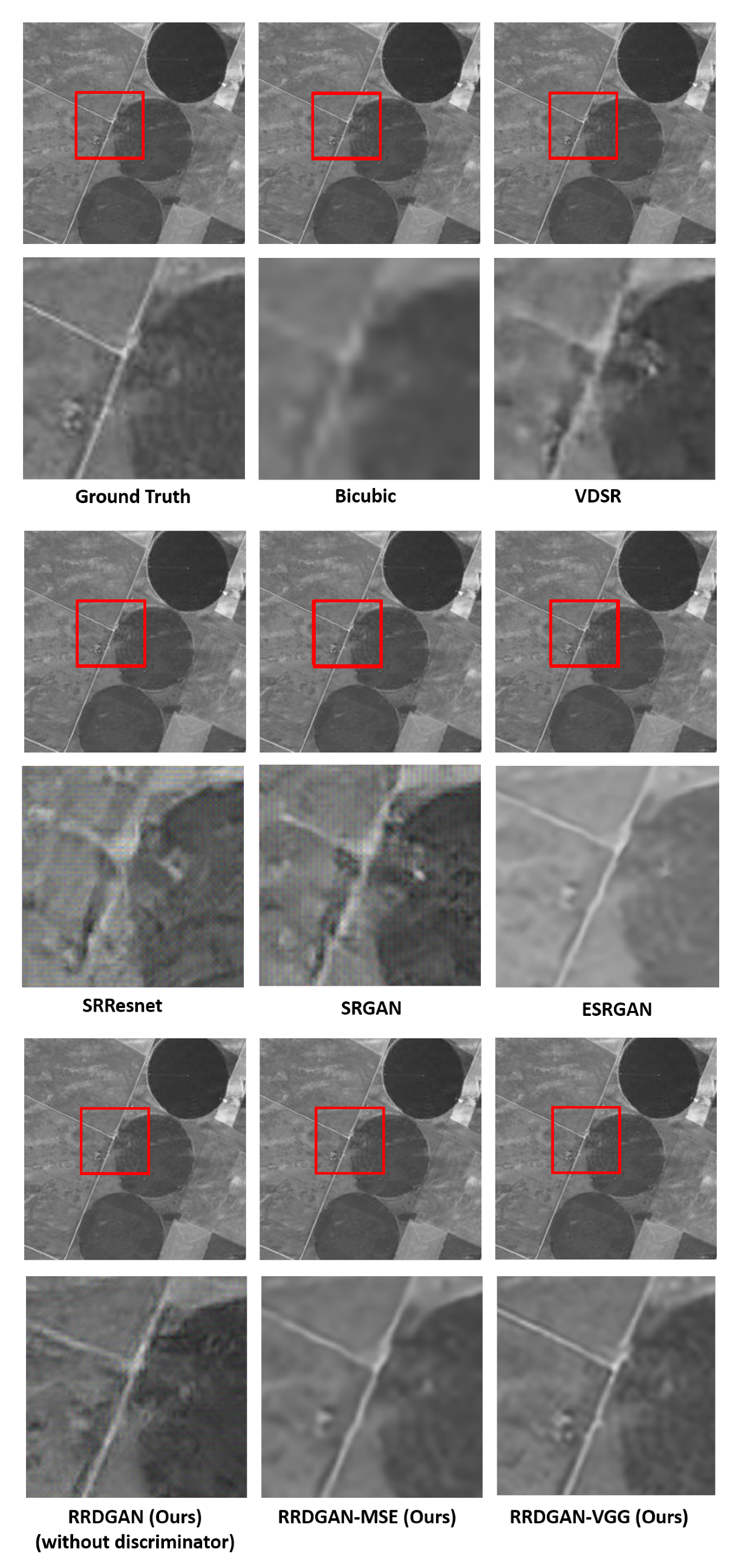
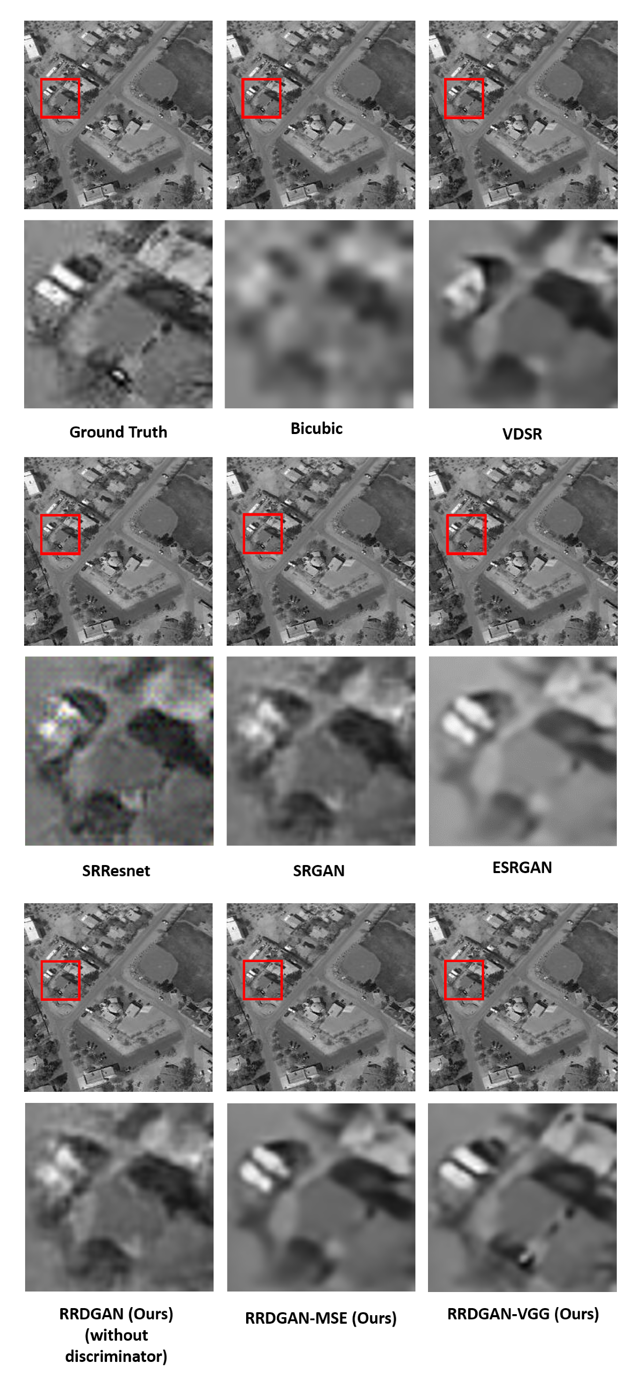
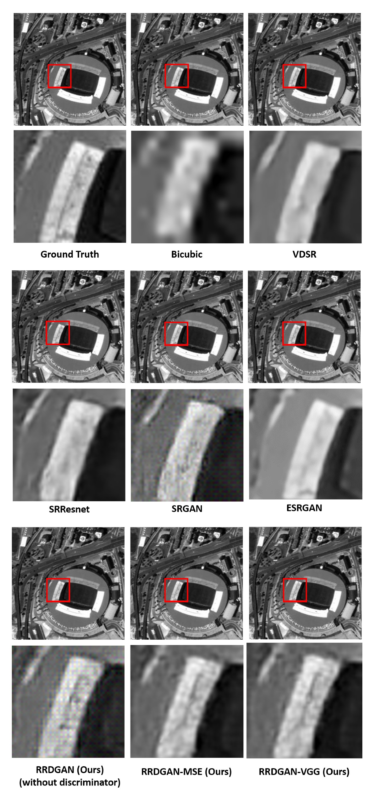
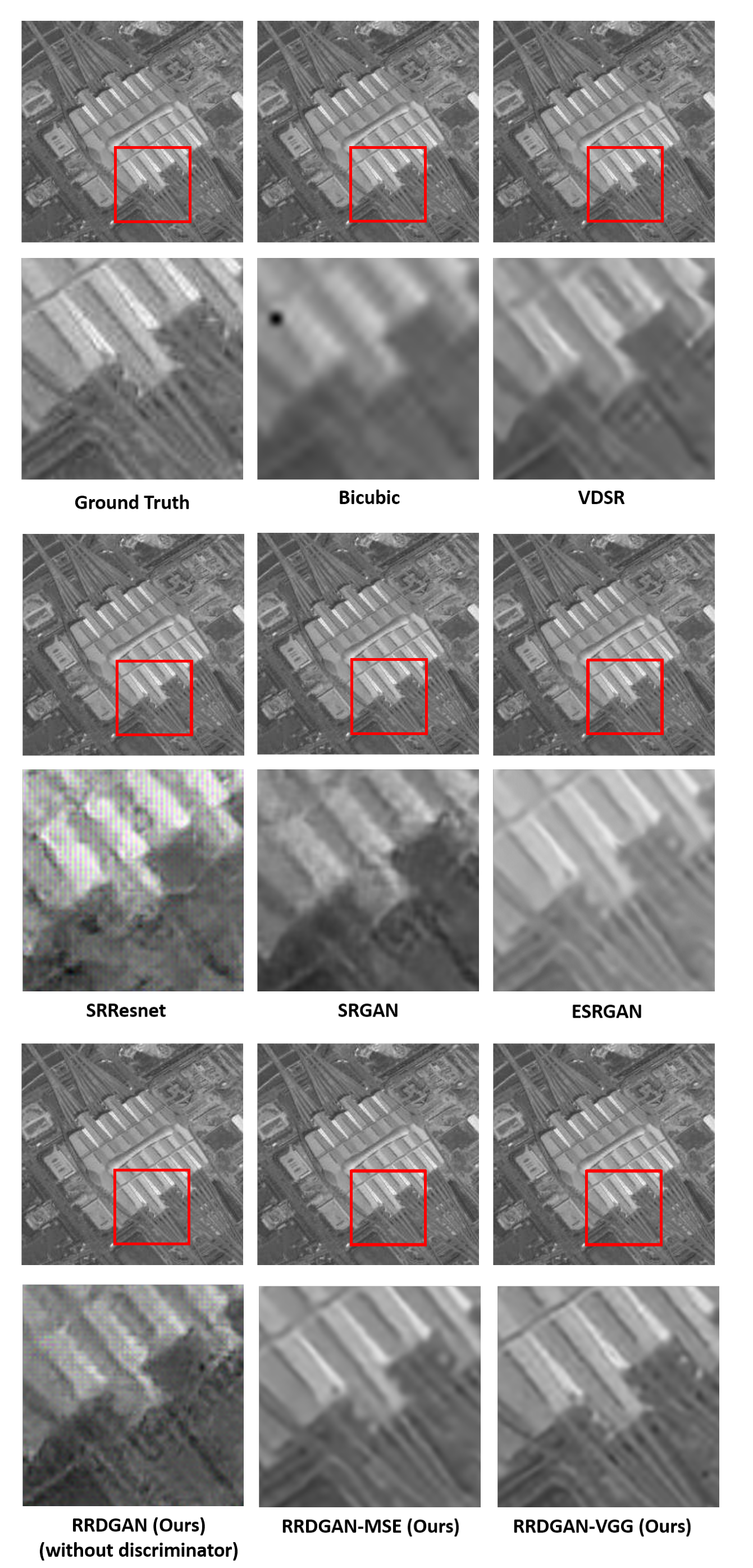
4.3. Results and Analysis

PSNR results and MOS of low resolution images with noise among our method, SRGAN, SRResnet and VDSR are illustrated in

Table 1. PSNR/MOS/Perceptual Index results (low resolution with noise) of applying methods to UCMERCED, NWPU-RESISC45 and GaoFen-1.

Scale	Bicubic	VDSR	SRResnet	SRGAN	ESRGAN	RRDGAN-MSE (Ours)	RRDGAN-VGG (Ours)
4	23.83/1.36/6.72	28.12/2.72/5.1	28.57/3/4.23	24.35/3.09/2.58	24.89/3.18/2.08	24.89/3.18/2.23	24.91/3.42/2.01
4	24.12/1.53/6.5	28.45/3.07/5.21	28.71/3.30/3.6	24.97/3.34/2.45	25.52/3.42/2.06	25.52/3.42/2.18	25.63/3.81/1.98

.

PSNR, short for “Peak Signal to Noise Ratio”, is an objective standard for image evaluation. It is generally used as an engineering project between the maximum signal and background noise.

$$PSNR=10{log}_{10}\frac{{\left(2^n-1\right)}^2}{MSE}$$

(8)

In Equation (8), n is the image bit width. The MSE is the mean square error, which is defined in Equation (9). X is the ground truth, and $F\left(Y\right)$ is the reconstructed image. M is the row number in X, and N is the column number in $F\left(Y\right)$.

$$MSE=\frac{{\sum }_{j=1}^N\left({\sum }_{i=1}^M{\left(F\left(Y_{i,j}\right)-X_{i,j}\right)}^2\right)}{MN}$$

(9)

MOS test has been used for decades. It was used to evaluate the quality of voice communication systems in the beginning, and later widely used to identify key components in voice communication systems. The MOS test process is a group of listeners sitting in a quiet room, listening to the call and scoring the call quality. Especially, inspired by SRGAN, 26 raters were asked to give an integral score from 1 (low) to 5 (high) to evaluate images reconstructed by different methods.

Another important metric to evaluate the reconstructed images is called perceptual index. Perceptual index is used to judge the perceptual quality of images. The definition of perceptual index is the expression of Ma’s score [40] and NIQE [41], which is showed in Equation (10). The lower perceptual index means a better reconstructed image.

$$perceptualindex=\frac{1}{2}\left(\left(10-M{a}^{\prime }sscore\right)+NIQE\right)$$

(10)

The result between our RRDGAN with VGG loss (RRDGAN-VGG) as its discriminator and RRDGAN with MSE loss (RRDGAN-MSE) as its discriminator were also compared int this table.

To further verify the performance of RRDGAN, we classify the results by the content of images. We totally use 10 classes of ground features to test.

Table 2. MEAN PSNR/MOS/Perceptual Index results (low resolution with white Gaussian noise) of each class in UCMERCED, NWPU-RESISC45 and GaoFen-1.

Class	Scale	Bicubic	VDSR	SRGAN	ESRGAN	RRDGAN-MSE (Ours)	RRDGAN-VGG (Ours)
airplane	4	23.46/1.53/6.44	28.04/2.73/4.36	24.23/3/2.53	24.92/3/2.11	24.89/3.11/2.20	25.00/3.42/2.02
baseballdiamond	4	24.12/1.63/6.35	28.45/2.73/4.35	24.31/3/2.35	25.04/3/2.08	25.01/3.19/2.21	25.11/3.57/1.90
beach	4	24.21/1.53/6.85	28.53/2.73/4.52	24.62/2.80/2.86	25.04/2.80/2.31	25.03/3.03/2.32	25.13/3.42/2.23
bridge	4	24.35/1.63/6.96	28.61/2.73/4.31	24.71/3.03/2.94	24.85/3.03/2.45	24.83/3.23/2.42	24.91/3.81/2.36
forest	4	23.75/1.63/6.53	28.72/2.84/4.25	24.72/3.09/2.51	25.09/3.09/2.34	25.08/3.26/2.38	25.14/3.42/2.20
groundtrack	4	21.34/1.82/7.69	25.34/2.73/5.12	21.98/3.07/3.34	22.07/3.07/2.95	22.11/3.18/3.00	22.35/3.57/2.98
intersection	4	23.45/1.53/6.45	28.04/2.63/4.86	24.24/3/2.68	24.56/3/2.35	24.52/3.36/2.45	24.63/3.42/2.26
mediumresidial	4	24.13/1.42/6.14	28.37/2.80/4.26	24.61/3.09/2.75	25.0/3.09/2.13	24.91/3.23/2.15	25.10/3.42/2.08
river	4	24.51/1.53/6.43	28.69/2.73/4.59	24.70/3.15/2.62	25.18/3.15/2.32	25.12/3.23/2.40	25.25/3.81/2.26
stadium	4	24.46/1.38/6.86	28.66/2.63/4.39	24.71/3/2.43	25.16/3/1.86	25.12/3.18/2.11	25.21/3.69/2.01

shows the results for these ground features. These results are reconstructions of low resolution with white Gaussian noise inputs. These results prove our RRDGAN has the best performance.

Figure 7, Figure 8, Figure 9, Figure 10 and Figure 11 illustrate some visual results (Low resolution with white Gaussian noise and low resolution with salt and pepper noise, respectively) of these methods. The HQ optical remote sensing images reconstructed by the RRDGAN-VGG have clearer details.

The influence of DBN numbers, BN and wavelet transform were also investigated, respectively, in our experiment. Among these three factors, we would discuss the influence of the number of DBN first. Figure 12 and Figure 13 are the experiment results of five different numbers of DBN on performance of PSNR and training time, respectively. We could see that PSNR is getting better with the increasing number of DBN. However, when the number of DBN is 25, the performance of PSNR is not significantly enhanced, while the training time is obviously increasing.

Then, we investigate the influence of BN. In this experiment, The result of using BN in the generative part and not using BN in the generative part were compared. We could see that not using BN is good for our method. BN only considers relative differences, and does not require absoluteness. It ignores absolute differences between pixels (or features) of the image (normalized variance because mean is zero). Differential tasks (such as categorization and recognition) have added value. Batch normalization does not perform well for image super-resolution reconstruction, which requires absolute difference. Figure 14 illustrates the influence of batch normalization.

Then, we discuss the influence of whether using wavelet transform. As illustrated in Figure 1 (LR with Gaussian noise), we could see that image restoration in wavelet transform domain achieves better performance.

For image SR reconstruction task, wavelet transform has been proven to have an ideal effect [42]. As Figure 15 shows, different frequency sub-bands represent different information of the image after wavelet decomposition, in which the low-frequency sub-bands represent the global topological information of the image, while the other high-frequency sub-bands represent the structure and texture of the image. Therefore, as long as the corresponding wavelet coefficients are accurately predicted, high-quality and high-resolution images with rich texture details and global topological information can be reconstructed from low-resolution images.

For image denoising, Gaussian noise and salt and pepper noise are two common noises in remote sensing images. For Gaussian noise, it exists in each frequency sub-band after Haar wavelet transform. Therefore, the removal of Gaussian noise is equivalent to learning the threshold information of traditional wavelet transform to remove Gaussian noise. After Haar wavelet transform, salt and pepper noise also exists in each frequency sub-band, and its shape and distribution are similar to the spatial domain. Therefore, the removal of salt and pepper noise is equivalent to learning the end-to-end relationship between noisy and noise-free images.

The effect of removing Gaussian noise in the wavelet transform domain is better than that in the spatial domain (just like Figure 1 shows), but the effect of removing salt and pepper noise in the wavelet transform domain is not significantly better than that in the spatial domain. This is because salt and pepper noise cannot be removed more easily in the domain of wavelet transform, so it is impossible to achieve a more ideal denoising effect through end-to-end learning. Figure 16 shows the comparison results of applying RRDGAN (only denoising) in both WT domain and spatial domain. We removed the upsampling part to make RRDGAN only accomplish the denoising task.

By the way, we also did some experiments to verify whether the performance of RRDGAN is better than implementing denoising method (BM3D Algorithm [43] or Non-Local Means method [44], which are two of the best denoising method) first, then SR method followed. Figure 17 shows the result that RRDGAN is better than using the combination of BM3D (or NLM) and RRDGAN. We can see that the result of the combination of BM3D (or NLM) and RRDGAN is smoother than the result of using RRDGAN directly.

Finally, we experimented to verify the effect of using relativistic loss and TV loss. Figure 18 and Figure 19 give the comparison results of whether to use relativistic loss and whether to use TV loss, respectively. We can see that using relativistic loss and TV loss helps to learn more details.

5. Discussions

5.1. Different from ESRGAN

Our method looks like ESRGAN, but there are still three differences between the two methods. Firstly, our RRDGAN uses TV loss to furthermore improve the quality of reconstructed image in generator part. Secondly, dense connection is the backbone of our RRDGAN, which has higher capacity, while ESRGAN uses residual learning as its backbone. Finally, our RRDGAN is implemented in WT domain, while ESRGAN is implemented in spatial domain. The experiment result shows that the performance of our RRDGAN is better than ESRGAN. In terms of computational complexity, we used bottleneck structure while ESRGAN did not. Each RRDGAN block almost has 290 M parameters, while each ESRGAN block has 4500M. So in one block, ESRGAN’s parameter number is almost 15 times ours.

5.2. Deal with White Gaussian Noise

Our method is implemented in WT domain, which could deal with SR and denoising problems in different frequency parts. In our experiment, Gaussian and salt and pepper noise are added, respectively, to the low resolution optical remote sensing image to obtain the final low quality image. Based on our analysis, SR and salt and pepper problems are both related to the high frequency part of optical remote sensing image, but white Gaussian noise exists in all frequency parts. So, handling white Gaussian noise in WT domain with deep learning method is to learn the different relationships in each frequency between low quality image and ground truth. The relationship obtained by our method is similar to the sparse decomposition result in using traditional WT-based denoising method. So after using the image with white Gaussian noise to train in WT domain, our RRDGAN could remove white Gaussian noise well.

5.3. Others

We add experiments to compare the super-resolution part of our method with Fractional Charlier moments method [10] and Hahn moments method [11] using database Set14 and AVLetters [45]. The experiment result shows that the super-resolution part of our method has better performance in both visual effect and quantitative result.

Figure 20 and Figure 21 are the results of experiment:

6. Conclusions

In this article, a GAN-based method implemented in WT domain named RRDGAN is proposed, which could solve both remote sensing image denoising and SR problems in the meantime by a unified network structure. RRDGAN mainly handles optical remote sensing image spatial denoising and super-resolution reconstruction problem in wavelet transform domain. It combines the advantages of both non-GAN-based and GAN-based methods, which means the generative part combines residual learning (includes both local and global residual learning) and dense connection to get a high PSNR result. Generator uses TV loss to furthermore enhance the reconstructed effect. Relativistic loss is also applied in our discriminator to make the whole network converge better. Finally, RRDGAN is implemented in WT domain instead of in spatial domain directly for the reason of different high frequency corresponding different detailed information, should be processed differently, which cannot be distinguished well in the spatial domain. The experimental results, which are tested on the datasets of UCMERCED, NWPU-RESISC45 and GAOFEN-1, show that our method not only could remove typical noise (salt & pepper noise and white gaussian noise) of remote sensing images but also could enhance the spatial resolution.

In the future, we would research a way to handle the problem that the quality of so-called remote sensing ground truth is also low. We will try to use high quality natural images to help us to accomplish this mission.

References

1. Xu, W.; Xu, G.; Wang, Y.; Sun, X.; Lin, D.; Wu, Y. Deep Memory Connected Neural Network for Optical Remote Sensing Image Restoration. Remote Sens. 2018, 10, 1893. [Google Scholar] [CrossRef] [Green Version]
2. Dong, C.; Loy, C.; He, K.; Tang, X. Learning a deep convolutional network for image super-resolution. In Proceedings of the European Conference on Computer Vision, Zurich, Switzerland, 6–12 September 2014; pp. 184–199. [Google Scholar]
3. Hou, H.; Andrews, H. Cubic spline for image interpolation and digital filtering. IEEE Trans. Image Process. 1978, 26, 508–517. [Google Scholar]
4. Dodgson, N. Quadratic interpolation for image resampling. IEEE Trans. Image Process. 1997, 6, 1322–1326. [Google Scholar] [CrossRef]
5. Huang, T.; Tsai, R. Multi-frame image restoration and registration. Adv. Comput. Vis. Image Process. 1984, 1, 317–339. [Google Scholar]
6. Kim, S.; Bose, N.; Valenauela, H. Recursive reconstruction of high resolution image from noisy undersampled multiframes. IEEE Trans. Acoust. Speech Signal Process. 1990, 38, 1013–1027. [Google Scholar] [CrossRef]
7. Shao, Z.; Wang, L.; Wang, Z.; Deng, J. Remote Sensing Image Super-Resolution Using Sparse Representation and Coupled Sparse Autoencoder. IEEE J. Sel. Top. Appl. Earth Obs. Remote Sens. 2019, 12, 2663–2674. [Google Scholar] [CrossRef]
8. Daoui, A.; Yamni, M.; Karmouni, H.; Sayyouri, M.; Qjidaa, H. Stable computation of higher order Charlier moments for signal and image reconstruction. Inf. Sci. 2020, 521, 251–276. [Google Scholar] [CrossRef]
9. Hmimid, A.; Sayyouri, M.; Qjidaa, H. Image classification using separable invariant moments of Charlier-Meixner and support vector machine. Multimed. Tools Appl. 2018, 77, 1–25. [Google Scholar] [CrossRef]
10. Yamni, M.; Daoui, A.; Karmouni, H.; Sayyouri, M.; Qjidaa, H.; Flusser, J. Fractional Charlier moments for image reconstruction and image watermarking. Signal Process. 2020, 171, 107509. [Google Scholar] [CrossRef]
11. Mesbah, A.; Berrahou, A.; Hammouchi, H.; Berbia, H.; Qjidaa, H.; Daoudi, M. Lip Reading with Hahn Convolutional Neural Networks. Image Vis. Comput. 2019, 88, 76–83. [Google Scholar] [CrossRef]
12. Li, F.; Xin, L.; Guo, Y.; Gao, D.; Kong, X.; Jia, X. Super-Resolution for GaoFen-4 Remote Sensing Images. IEEE Geosci. Remote Sens. Lett. 2015, 15, 28–32. [Google Scholar] [CrossRef]
13. Huang, G.; Zhuang, L.; Maaten, L. Densely Connected Convolutional Networks. In Proceedings of the IEEE Conference on Computer Vision and Pattern Recognition, Honolulu, HI, USA, 21–26 July 2017; pp. 4700–4708. [Google Scholar]
14. Feng, X.; Su, X.; She, J.; Jin, H. Single Space Object Image Denoising and Super-Resolution Reconstructing Using Deep Convolutional Networks. Remote Sens. 2019, 11, 1910. [Google Scholar] [CrossRef] [Green Version]
15. Glasner, D.; Bagon, S.; Irani, M. Super-resolution from a single image. In Proceedings of the IEEE International Conference on Computer Vision, Kyoto, Japan, 29 September–2 October 2009. [Google Scholar]
16. Yang, J.; Wright, J.; Huang, T.; Ma, Y. Image super-resolution via sparse representation. IEEE Trans. Image Process. 2010, 19, 2861–2873. [Google Scholar] [CrossRef]
17. Pérez-Pellitero, E.; Salvador, J.; Ruiz-Hidalgo, J.; Rosenhahn, B. PSyCo: Manifold span reduction for super resolution. In Proceedings of the IEEE Conference on Computer Vision and Pattern Recognition, Las Vegas, NV, USA, 27–30 June 2016; pp. 1837–1845. [Google Scholar]
18. Timofte, R.; De Smet, V.; Van Gool, L. PSyCo: A+: Adjusted anchored neighborhood regression for fast super-resolution. In Proceedings of the Asian Conference on Computer Vision, Singapore, 1–5 November 2014; pp. 111–126. [Google Scholar]
19. Salvador, J.; Pérez-Pellitero, E. Naive Bayes super-resolution forest. In Proceedings of the IEEE International Conference on Computer Vision, Santiago, Chile, 11–18 December 2015; pp. 325–333. [Google Scholar]
20. Song, H.; Liu, Q.; Wang, G.; Hang, R.; Huang, B. Spatiotemporal Satellite Image Fusion Using Deep Convolutional Neural Networks. IEEE J. Sel. Top. Appl. Earth Obs. Remote Sens. 2018, 11, 821–829. [Google Scholar] [CrossRef]
21. Kanakaraj, S.; Nair, M.S.; Kalady, S. SAR Image Super Resolution using Importance Sampling Unscented Kalman Filter. IEEE J. Sel. Top. Appl. Earth Obs. Remote Sens. 2018, 11, 562–571. [Google Scholar] [CrossRef]
22. Dong, C.; Loy, C.; He, K.; Tang, X. Image super-resolution using deep convolutional networks. IEEE Trans. Pattern Anal. Mach. Intell. 2016, 38, 295–307. [Google Scholar] [CrossRef] [Green Version]
23. Kim, J.; Lee, J.; Lee, K. Accurate Image Super-Resolution Using Very Deep Convolutional Networks. In Proceedings of the IEEE Conference on Computer Vision and Pattern Recognition, Las Vegas, NV, USA, 27–30 June 2016; pp. 142–149. [Google Scholar]
24. Ledig, C.; Theis, L.; Huszar, F.; Caballero, J.; Cunningham, A.; Acosta, A.; Aitken, A.; Tejani, A.; Totz, J.; Wang, Z.; et al. Photo-Realistic Single Image Super-Resolution Using a Generative Adversarial Network. In Proceedings of the IEEE Conference on Computer Vision and Pattern Recognition, Honolulu, HI, USA, 21–26 July 2017. [Google Scholar]
25. Wang, X.; Yu, K.; Wu, S.; Gu, J.; Liu, Y.; Dong, C. Esrgan: Enhanced super-resolution generative adversarial networks. In Proceedings of the European Conference on Computer Vision Workshops, Munich, Germany, 8–14 September 2018. [Google Scholar]
26. Mahendran, A.; Vedaldi, A. Understanding Deep Image Representations by Inverting Them. In Proceedings of the IEEE Conference on Computer Vision and Pattern Recognition, Columbus, OH, USA, 24–27 June 2014. [Google Scholar]
27. Rudin, L.I.; Osher, S.; Fatemi, E. Nonlinear total variation based noise removal algorithms. Phys. Nonlinear Phenom. 1992, 60, 259–268. [Google Scholar] [CrossRef]
28. Alexia, J.-M. The relativistic discriminator: A key element missing from standard GAN. arXiv 2018, arXiv:1807.00734. [Google Scholar]
29. Lai, W.S.; Huang, J.B.; Ahuja, N.; Yang, M.H. Deep Laplacian Pyramid Networks for Fast and Accurate Super-Resolution. In Proceedings of the IEEE Conference on Computer Vision and Pattern Recognition, Honolulu, HI, USA, 21–26 July 2017; pp. 5835–5843. [Google Scholar]
30. Tong, T.; Li, G.; Liu, X.; Guo, Q. Image Super-Resolution Using Dense Skip Connections. In Proceedings of the IEEE Conference on Computer Vision and Pattern Recognition, Honolulu, HI, USA, 21–26 July 2017; pp. 4700–4708. [Google Scholar]
31. Jain, V.; Seung, H. Natural image denoising with convolutional networks. In Proceedings of the Advances in Neural Information Processing Systems, Vancouver, BC, Canada, 8–10 December 2008; pp. 769–776. [Google Scholar]
32. Zhang, K.; Zuo, W.; Chen, Y.; Meng, D.; Zhang, L. Beyond a Gaussian Denoiser: Residual Learning of Deep CNN for Image Denoising. IEEE Trans. Image Process. 2017, 26, 3142–3155. [Google Scholar] [CrossRef] [Green Version]
33. Mao, X.; Shen, C.; Yang, Y. Image Restoration Using Convolutional Auto-encoders with Symmetric Skip Connections. arXiv 2016, arXiv:1606.08921. [Google Scholar]
34. Nhat, N.; Peyman, M. A Wavelet-Based InterpolationRestoration Method For Superresolution (Wavelet Superresolution). Circuits Syst. Signal Process. 2000, 19, 321–338. [Google Scholar]
35. Yang, J.; Zhao, Y.; Chan, J.; Xiao, L. A Multi-Scale Wavelet 3D-CNN for Hyperspectral Image Super-Resolution. Remote Sens. 2019, 11, 1557. [Google Scholar] [CrossRef] [Green Version]
36. Chen, Y.; Li, J.; Xiao, H.; Jin, X.; Yan, S.; Feng, J. Dual Path Network. arXiv 2017, arXiv:1707.01629. [Google Scholar]
37. Shi, W.; Caballero, J.; Huszar, F.; Totz, J.; Aitken, A.P.; Bishop, R. Real-time single image and video super-resolution using an efficient sub-pixel convolutional neural network. In Proceedings of the IEEE Conference on Computer Vision and Pattern Recognition, Las Vegas, NV, USA, 27–30 June 2016. [Google Scholar]
38. Yang, Y.; Newsam, S. Bag-of-visual-words and spatial extensions for land-use classification. In Proceedings of the 18th SIGSPATIAL International Conference On Advances in Geographic Information Systems, San Jose, CA, UAS, 2–5 November 2010; pp. 270–279. [Google Scholar]
39. Cheng, G.; Han, J.; Lu, X. Remote sensing image scene classification: Benchmark and state of the art. Proc. IEEE 2017, 105, 1865–1883. [Google Scholar] [CrossRef] [Green Version]
40. Ma, C.; Yang, C.Y.; Yang, X.; Yang, M.H. Learning a no-reference quality metric for single-image super-resolution. CVIU 2017, 158, 1–16. [Google Scholar] [CrossRef] [Green Version]
41. Mittal, A.; Soundararajan, R.; Bovik, A.C. Making a completely blind image quality analyzer. IEEE Signal Process. Lett. 2013, 20, 209–212. [Google Scholar] [CrossRef]
42. Huang, H.; He, R.; Sun, Z.; Tan, T. Wavelet-SRNet: A Wavelet-Based CNN for Multi-scale Face Super Resolution. ICCV 2017, 2, 175–213. [Google Scholar]
43. Lebrun, M. An analysis and implementation of the BM3D image denoising method. Image Process. Line 2012, 2, 175–213. [Google Scholar] [CrossRef] [Green Version]
44. Buades, A.; Coll, B.; Morel, J.M. Non-Local Means Denoising. Image Process. Line 2011, 1, 208–212. [Google Scholar] [CrossRef] [Green Version]
45. Matthews, I.; Cootes, T.F.; Bangham, J.A.; Cox, S.; Harvey, R. Extraction of visual features for lipreading. IEEE Trans. Pattern Anal. Mach. Vis. 2002, 24, 198–213. [Google Scholar] [CrossRef]
Figure 1. The comparison of implementing our method in WT domain or in spatial domain.
Remotesensing 13 01858 g001
Figure 2. The flowchart of Haar wavelet transform.
Remotesensing 13 01858 g002
Figure 3. The main steps of the generative part in RRDGAN.
Remotesensing 13 01858 g003
Figure 4. The architecture of RRDGAN.
Remotesensing 13 01858 g004
Figure 5. Low resolution with White Gaussian noise input.
Remotesensing 13 01858 g005
Figure 6. Low resolution with salt and pepper noise input.
Remotesensing 13 01858 g006
Figure 7. Comparison results among different methods of “Airplane”, scale factor is 4.
Remotesensing 13 01858 g007
Figure 8. Comparison results among different methods of “CircularFarmland”, scale factor is 4.
Remotesensing 13 01858 g008
Figure 9. Comparison results among different methods of “BaseballDiamond”, scale factor is 4.
Remotesensing 13 01858 g009
Figure 10. Comparison results among different methods of “Stadium”, scale factor is 4.
Remotesensing 13 01858 g010
Figure 11. Comparison results among different methods of “Railway”, scale factor is 4.
Remotesensing 13 01858 g011
Figure 12. The influence of DBN numbers on performance of PSNR.
Remotesensing 13 01858 g012
Figure 13. The influence of DBN numbers on performance of training time.
Remotesensing 13 01858 g013
Figure 14. The influence of batch normalization.
Remotesensing 13 01858 g014
Figure 15. Wavelet transform schematic diagram of image with salt and pepper noise.
Remotesensing 13 01858 g015
Figure 16. Comparison results of Applying RRDGAN (only denoising) in both WT domain and spatial domain.
Remotesensing 13 01858 g016
Figure 17. Comparison results of implementing BM3D (or NLM) and RRDGAN and implementing RRDGAN only.
Remotesensing 13 01858 g017
Figure 18. Comparison results of whether using relativistic loss or not.
Remotesensing 13 01858 g018
Figure 19. Comparison results of whether using TV loss or not.
Remotesensing 13 01858 g019
Figure 20. Comparing the super-resolution part of our method with Fractional Charlier moments using Set14.
Remotesensing 13 01858 g020
Figure 21. Comparing the super-resolution part of our method with Hahn moments using AVLetters.
Remotesensing 13 01858 g021