
Analysis of Activity in an Open-Pit Mine by Using InSAR Coherence-Based Normalized Difference Activity Index


Department of Geophysics, Kangwon National University, Chuncheon-si 24341, Korea
*
Author to whom correspondence should be addressed.
Remote Sens. 2021, 13(9), 1861; https://0-doi-org.brum.beds.ac.uk/10.3390/rs13091861
Submission received: 1 April 2021
/
Revised: 28 April 2021
/
Accepted: 7 May 2021
/
Published: 10 May 2021
(This article belongs to the Special Issue Selected Papers from the “International Symposium on Remote Sensing 2021”)
Abstract
:In this study, time-series of Sentinel-1A/B Interferometric Synthetic Aperture Radar (InSAR) coherence images were used to monitor the mining activity of Musan open-pit mine, the largest iron mine in North Korea. First, the subtraction of SRTM DEM (2000) from TanDEM-X DEM (2010–2015) has identified two major accumulation areas, one in the east (+112.33 m) and the other in the west (+84.03 m), and a major excavation area (−42.54 m) at the center of the mine. A total of 89 high-quality coherence images with a 12-day baseline from 2015 to 2020 were converted to the normalized difference activity index (NDAI), a newly developed activity indicator robust to spatial and temporal decorrelation. An RGB composite of annually averaged NDAI maps (red for 2019, green for 2018, and blue for 2017) showed that overall activity has diminished since 2018. Dumping slopes were categorized into shrinking, expanding, or transitional, according to the color pattern. Migration and expansion of excavation sites were also found on the pit floor. Time series of 12-day NDAI graphs revealed the date of activities with monthly accuracy. It is believed that NDAI with continuous acquisition of Sentinel-1A/B data can provide detailed monitoring of various types of activities in open-pit mines especially with limited in situ data.

1. Introduction
Surface mining refers to a method of excavating ore deposits from the surface and is preferred to underground mining for large-scale ore development [1]. Abrupt surface change occurs in the surface mining site, such as deforestation, ecological destruction [2,3], desertification [4,5], and hydrological disruptions [6,7,8]. It is required to monitor surface mines constantly to investigate the ecological and hydrological impact of mining activities as well as economical activities especially in restricted areas where direct information is scarce.
Remote sensing is useful for studies observing surface changes caused by the mining activities. Various techniques have been developed in studies to identify mining areas or to detect changes in land cover. For example, LaJeunesse Connette et al. [9] calculated the mining area using reflectance data acquired from Landsat images. Julzarika [10] identified the mining area through vegetation index differencing. Lobo et al. [11] confirmed the mining area by applying supervised classification to Sentinel-2A and RapidEye images. The study using digital elevation model (DEM) data to confirm that mining is also a topic of interest to many researchers. Ross et al. [12] used LiDAR to generate high-resolution elevation data and confirmed the elevation change before and after mine activity. Lee [13] estimated the mining depth by differentiating the DEM extracted from the KOMPSAT-5 Synthetic Aperture Radar (SAR) interferogram from the Shuttle Radar Topography Mission (SRTM) DEM [14]. Wu et al. [15] improved detection accuracy using Landsat data while performing an elevation analysis based on DEM data. Wang et al. [16] detected the location of legal and illegal mining activities by extracting the decorrelation area based on the coherence map and overlaying it on the mining rights distribution maps.
Among various study methods, SAR-based remote sensing has the advantage of enabling continuous observation regardless of sunlight and cloud conditions. SAR data have been widely used in land subsidence [17], landslides [18], power towers [19], power line corridors [20], and earthquakes studies [21]. Particularly, Interferometric SAR (InSAR) coherence, which can detect random changes on the surface, is effective in the study of mines where activity occurs on the surface. Coherence has a value between 0 and 1 and represents the stability of surface. A stable surface will have coherence values near 1, while the decorrelation of random scattering will have coherence values close to 0 [22]. Bare land, rocks, outcrops, and buildings in urban areas have very high coherence values because they have almost no movement and only surface scattering exits. Vegetated areas or forest, on the other hand, have low coherence values due to volume scattering (volume decorrelation) and changes affecting the scatters within the resolution cell (temporal decorrelation) [23]. In an open-pit mine, topsoil is removed and vegetation is hardly distributed in the mining area. Therefore, the coherence value is relatively high over the open-pit except for the area of mining activities such as blasting, excavation, and accumulation.
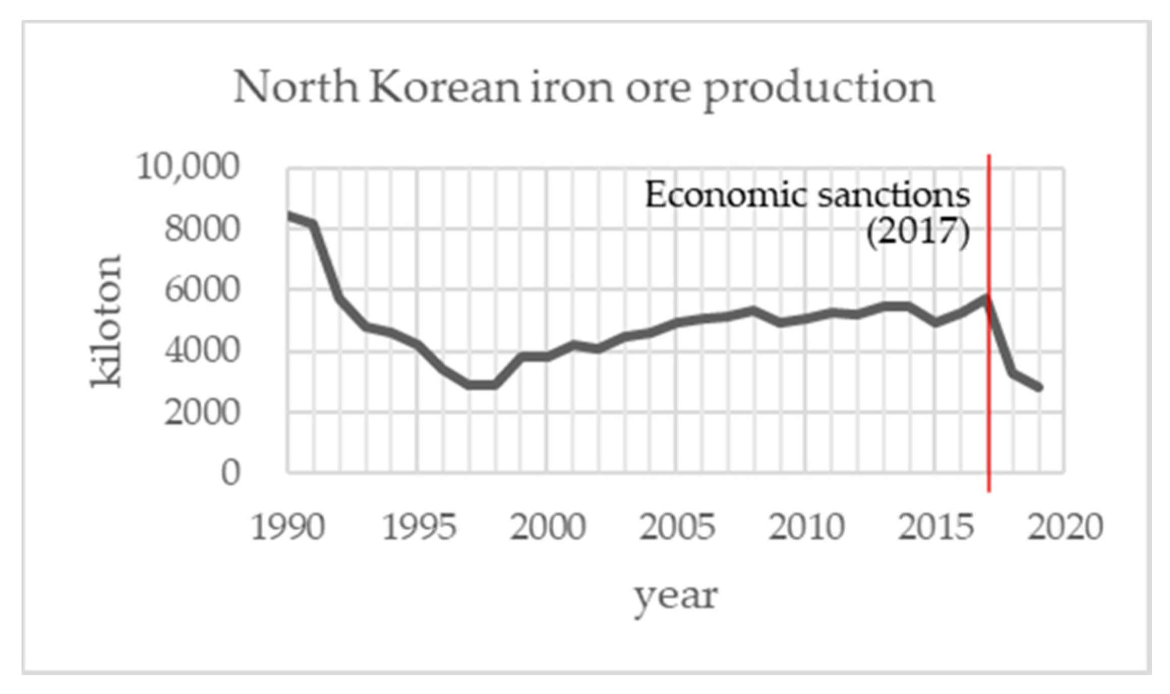
The purpose of this study is to observe the activity of Musan open-pit mine, where the in situ measurement is hard to obtain, using remote sensing techniques. According to the Korean Statistical Information Service (KOSIS), North Korea’s iron ore production is estimated to have declined due to economic sanctions from 2017 (Figure 1) [24]. Musan open pit, a major mine that accounts for most of North Korea’s iron ore production, is expected to have had a decreasing production since then. The reduction in production also came from the aging infrastructure. To overcome this problem through cooperation between South Korea and North Korea, many studies have been actively conducted recently in various fields, such as mining industry [25], resources [26,27], deposits [28], mine hazards [29], landslide susceptibility [30], and infrastructure development [31,32].
In this study, two InSAR DEM datasets were used to identify the major elevation changes due to mining activities between 2000 and 2015. Activities for the recent 5 years (2015–2020) were identified using Sentinel-1 InSAR coherence time-series data with a 12-day temporal baseline. A new index, so called the Normalized Difference Activity Index (NDAI), has been developed to highlight the activities and to mitigate decorrelation from other sources, such as precipitation or spatial baseline. Section 2 introduces the study area, data, and methods including the newly developed NDAI. Section 3 presents the research results and discussions, which includes the analysis of NDAI images over all periods, annual variations, and activities that occurred during the 12-day InSAR baseline. Section 4 concludes the paper, highlighting the major findings.
2. Materials and Methods
2.1. Study Area
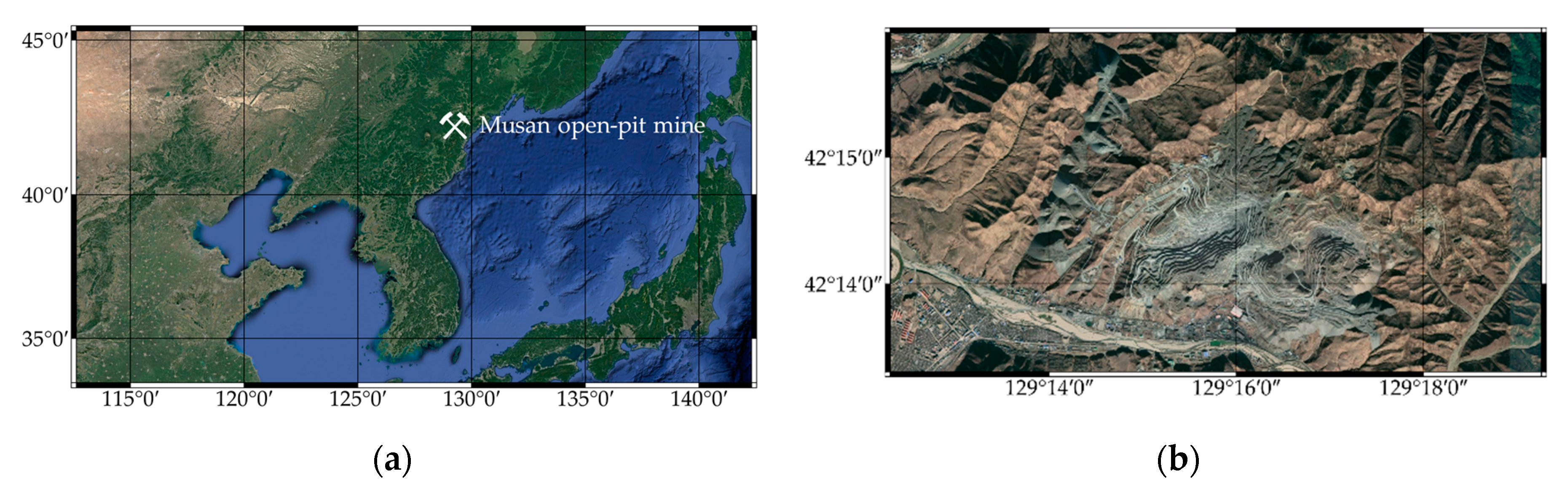
The study area is Musan open-pit mine, North Korea, close to the Chinese border (Figure 2). Musan mine is an iron-magnetite mine located in Musan-gun, North Hamgyeong Province, with a center location of 42°14′05″N, 129°15′21″E [26]. Open-pit mining refers to the process of mining the deposit near the surface by pitting benches through blasting [33]. In thick deposits, a large number of benches are required to reach the desired depth. The approximate diameter of the mine is 4 km with an area of 15 km2. Due to the limited access to the in situ data, remote sensing is the major source of information to analyze the activity of the mine. The Musan mine began production at the earliest from 1937 [34]. The existing reserves of the mine were estimated to be about 1.5 billion tons [27,35,36]. The grade of raw ore is 25–35%, and the grade of ore concentrate is 65% [37].
2.2. Data
2.2.1. SRTM and TanDEM-X DEM
Open-pit mining activities produce a large amount of surface elevation change due to excavation at mining sites and accumulation at dumping sites. As elevation changes in the accumulation and excavation areas are directly exposed on the surface, the mining activity can be inferred through the change in elevation by subtracting the DEMs obtained with a time gap. Therefore, the mining activity can be detected by elevation difference from two DEMs obtained before and after it. Bae et al. [26] investigated the elevation change at Musan mine between 1976 and 2007 based on optical satellite data. As seen in Figure 1, there was an increase in production at the Musan mine from about 2000 before its decrease after 2017; the elevation difference between an earlier DEM and a recent one can demonstrate the accumulation and excavation of the mining area. In this study, the earlier DEM is selected as the Shuttle Radar Topography Mission (SRTM) data acquired by National Geospatial Intelligence Agency (NGA) and National Aeronautics and Space Administration (NASA) in 2000 [14], and the recent one is selected as TerraSAR-X add-on for Digital Elevation Measurement (TanDEM-X) data acquired by Deutsches Zentrum für Luft und Raumfahrt, German Aerospace Center (DLR) from 2010–2015 [38].
SRTM DEM were obtained from C-band SAR data operated by the space shuttle Endeavour from 11 to 22 February, 2000. The fixed baseline single-pass spaceborne InSAR technology system was first introduced through SRTM [14]. In this study, SRTM 1 arc-second DEM were used. TanDEM-X satellite was launched on 21 June, 2010, on a mission to create the latest global InSAR DEM with consistent and high precision [39,40,41]. The TanDEM-X satellite is operated with the TerraSAR-X satellite launched earlier on 15 June, 2007 at a baseline interval of 300–500 m. Data were collected from 2010 to 2015 in a bistatic configuration, and high-resolution world DEM images were generated in 2016. We used the TanDEM-X 90m DEM released freely in September 2018, which is a global DEM with a spatial resolution of 3 arc-seconds created by reducing the pixel spacing of the existing TanDEM-X DEM with 0.4 arc-seconds resolution.
For DEM analysis, TDM1_DEM__30_N42E129 data and SRTM1N42E129V3 data were used. Both data have a spatial coverage of 42–43°N and 129–130°E. TDM1_DEM__30_N42E129 data were created on 13 June, 2015 with a total of 72 scenes acquired on 26 dates from 4 September 2011 to 28 August 2014. SRTM1N42E129V3 data were acquired on 11 February 2000 and updated on 2 January 2015.
2.2.2. Sentinel-1 SAR
Sentienel-1 SAR data were used to observe the latest mining activity in time series since 2015. Operated by the European Space Agency (ESA), Sentinel-1A/B are equipped with a C-band SAR system and provide near-global coverage [42]. The Sentinel-1A was launched on 2 April 2014 and the Sentinel-1B was on 25 April 2016. The two satellites share the same orbit, and each has a repetition period of 12 days. As the two satellites are 180° apart in orbital plane, SAR images can be acquired at intervals of 6 days at the shortest [42]. In this study, a total of 134 Sentinel-1A/B SAR images were acquired from 11 June 2015 to 9 May 2020, mostly with a 12-day temporal baseline. Single look complex (SLC) images were used to generate InSAR coherence images from data obtained in interferometric wide (IW) swath mode in descending track. IW is the main acquisition mode of Sentinel-1A/B on land for a long time-series dataset where images are acquired and merged into three sub-swaths using the terrain observation with progressive scans (TOPS) SAR technique [42,43]. It has a wide swath of 250 km with the spatial resolution of 5 m in range and 20 m in azimuth. SLC products are generally updated within 3 h of data acquisition, and all data can be downloaded freely from the Copernicus Open Access Hub [44] and Alaska Satellite Facility (ASF) [45].
2.3. Methods
2.3.1. Subtraction of DEMs
The elevation change was calculated by subtracting the TanDEM-X 90 m DEM data and the SRTM 1 arc-sec HGT DEM data. Data processing was performed using SNAP (ESA’s SentiNel Application Platform) [46]. SNAP is an open-source common architecture for ESA Toolboxes ideal for the exploitation of Earth Observation data. SNAP Sentiel-1 Toolbox (S1TBX), an open source toolbox for Sentinel-1 SAR data, also supports a variety of SAR missions such as ALOS-1/2, Cosmo-Skymed, ENVISAT, ERS-1/2, KOMPSAT-5, Radarsat-1/2, TanDEM-X, and TerraSAR-X. The TanDEM-X DEM data were resampled by the bilinear interpolation method, and the two images were stacked so that the spatial resolution of the TanDEM-X 90 m DEM and the SRTM 1 arc-sec DEM matched. The two DEM data were then subtracted to derive the elevation. Although we cannot specify the date of TanDEM-X DEM data, because it was generated based on data acquired from 2011 to 2014, it is possible to confirm the change in elevation over a decade when compared with the SRTM DEM data obtained in 2000.
2.3.2. InSAR Coherence
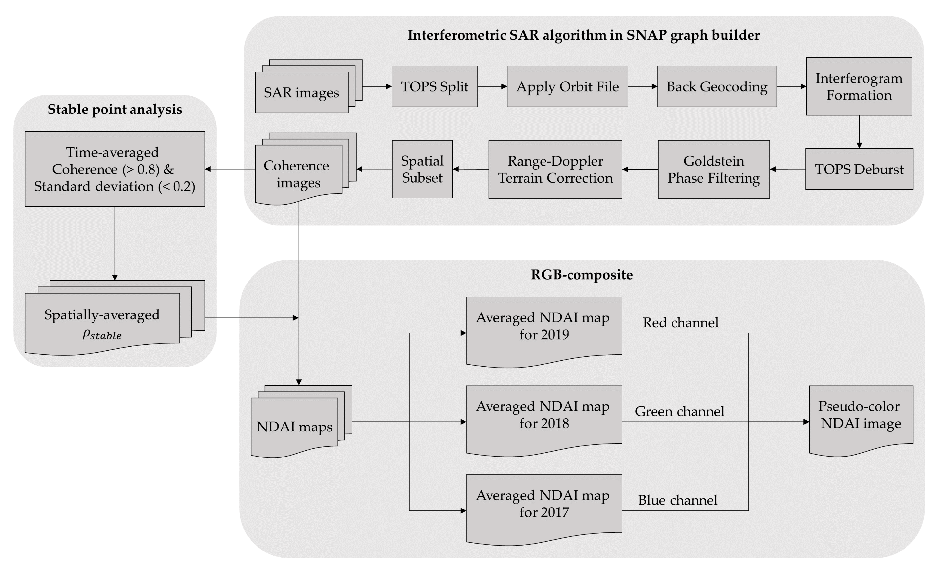
Out of the 134 SAR images, 25 images from 11 June 2015 to 24 May 2016 were acquired by Sentinel-1A and 109 images from 27 September 2016 to 9 May 2020 were by Sentinel-1B. Images between 24 May 2016 and 27 September 2016 were missing due to a change in the image acquisition plan from ESA. S1TBX was used for SAR and InSAR processing. Figure 3 shows a batch-processed InSAR process constructed by a graph builder tool in SNAP to utilize a pair of Sentinel-1 InSAR pairs as inputs to generate an interferogram and coherence map. In this processing, the orbit data were updated to Sentinel precise orbit to reduce the orbit error range to less than 10 cm. Two SAR datasets were co-registered by a back-geocoding tool. In the interferogram tool, the ellipsoidal earth phase and topographic phase were removed by using SRTM 1 arc-sec DEM data. The coherence was estimated by using an averaging window of 7 × 2 in range and azimuth, respectively. Goldstein phase filtering was applied to reduce speckle noise in the interferogram, and the data are written to finish the graph builder tool. A total of 126 coherence images with 12-day intervals were generated for further analysis (Figure 4). As a post-processing time series, coherence images can be stacked to generate average and standard deviation of coherence in time for each pixel, if necessary. To display the coherence images in Google Earth for further analysis, terrain correction and geocoding were applied to generate an orthorectified coherence image. The region of interest was subset from the image to reduce the file size before being exported to Google Earth KMZ format.
There are many causes of phase decorrelation that affect coherence [47,48,49,50]. In this study, we focus on the coherence and decorrelation factors as follows:
Here, indicates the temporal decorrelation from mining activity, the aim of this research. is related to decorrelation due to precipitation conditions, such as snow fall or rain event. is related to decorrelation from the perpendicular baseline of an InSAR pair. We try to analyze the behavior of the unwanted decorrelation factors ( and ) on stable points that were not affected by mining activity and find a way to statistically mitigate noise and highlight by introducing a new indexing method as follows.
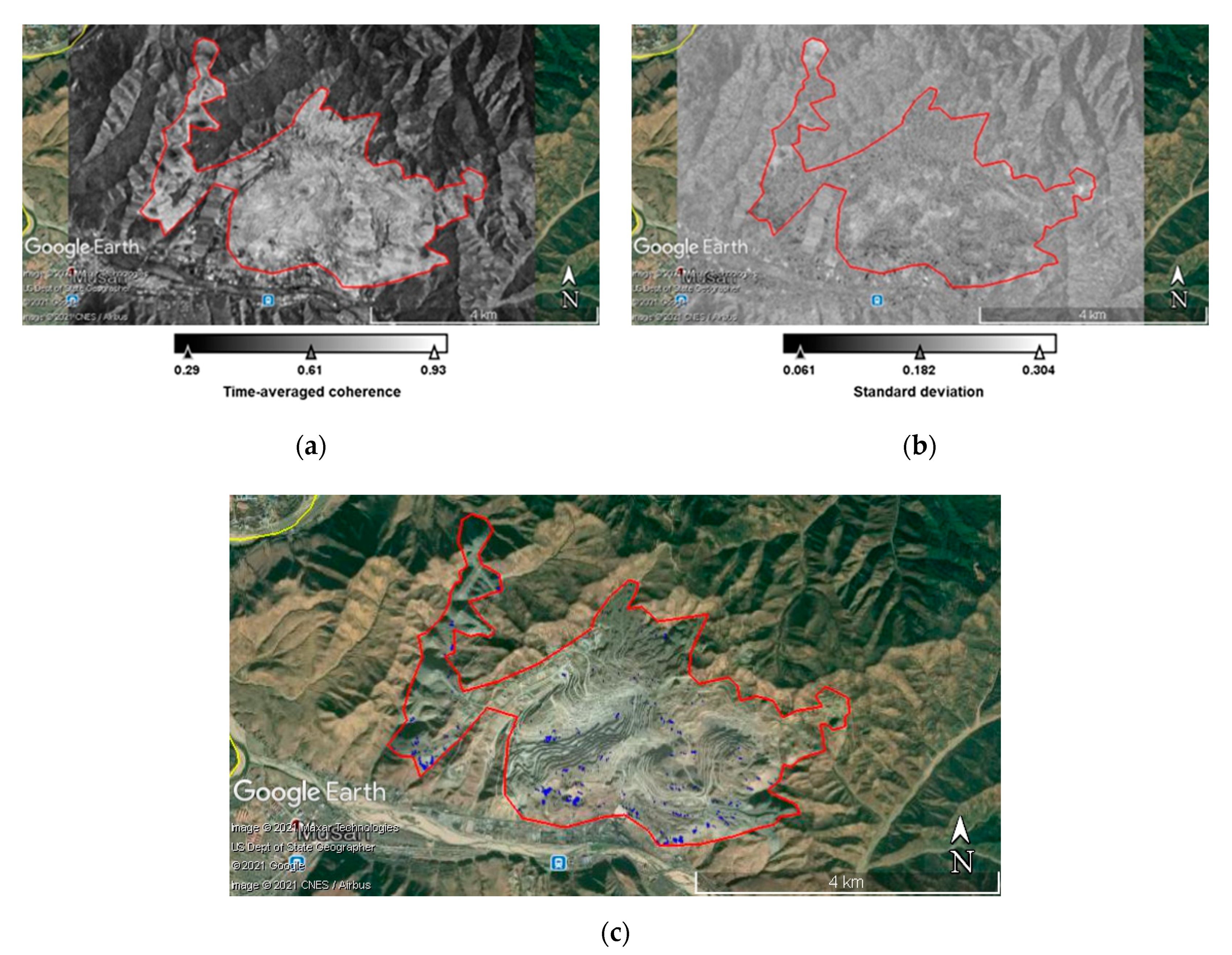
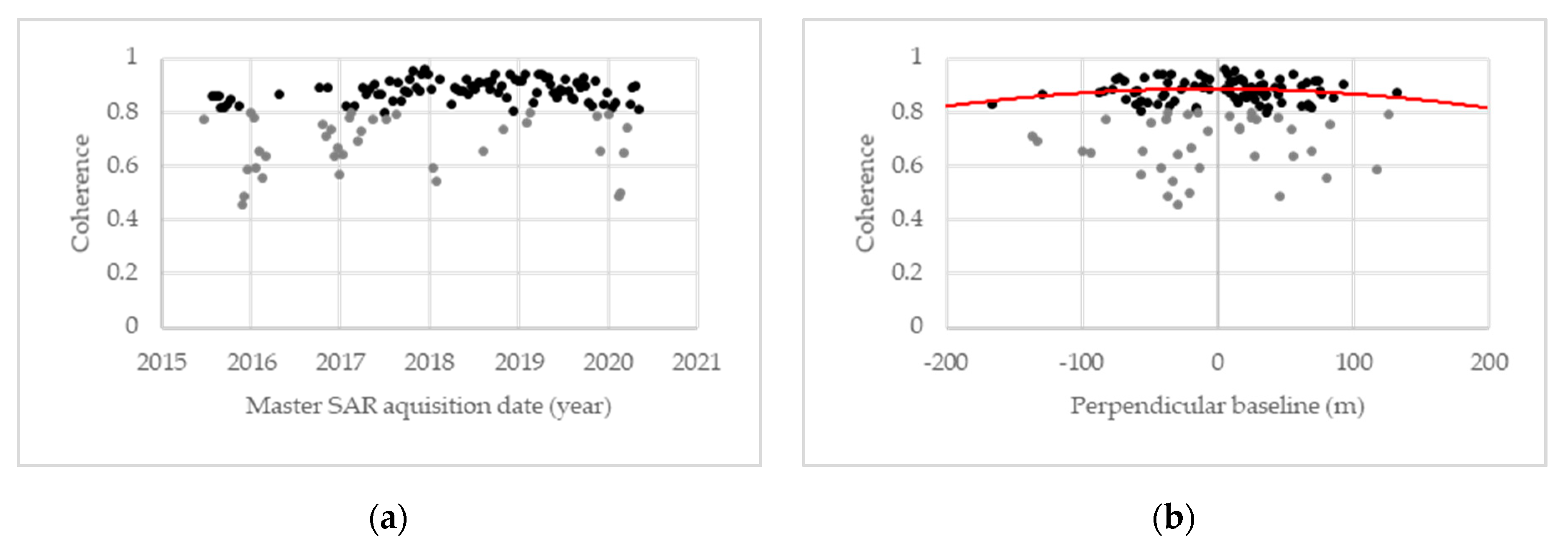
To analyze the effect of and , we generated a time-averaged coherence image over the study duration (Figure 5a) and its standard deviation (Figure 5b). Stable points in the mining area were selected (Figure 5c) by choosing pixels with time-averaged coherence values over 0.8 and standard deviation less than 0.2. In Figure 6a, the spatially averaged coherence values for those stable points ( were depicted as a function of time. It is interesting to see that low coherence values occur almost in winter time probably due to snow fall events. We decided to exclude the coherence image with a value less than 0.8 for further analysis, as depicted in light gray dots in Figure 6a. By doing so, the effect of is believed to be mitigated to some degree. A total of 89 coherence images out of 126 have survived the 0.8 criterion. Figure 6b shows the regression of spatially averaged coherence values of stable points with the perpendicular baselines. It shows that spatial decorrelation due to perpendicular baseline, , still exists after earth flattening and topographic removal operation that hinders the use of coherence as a measure of surface activity change. This is a spatial decorrelation regardless of the target property, which can be adjusted by the following method.
2.3.3. Normalized Difference Activity Index (NDAI)
We simplify Equation (1) by merging and as noise so that
We now define a new indexing method, so called the Normalized Difference Activity Index (NDAI), to reduce the noise signal by utilizing stable points.
Here, is the spatially averaged coherence value of stable points as defined above. is the coherence value of the target of interest. Since and , NDAI can be expressed as follows:
Based on the assumption that and is irrespective of target properties so that , NDAI can mitigate the noise signal and represents surface activity only as follows:
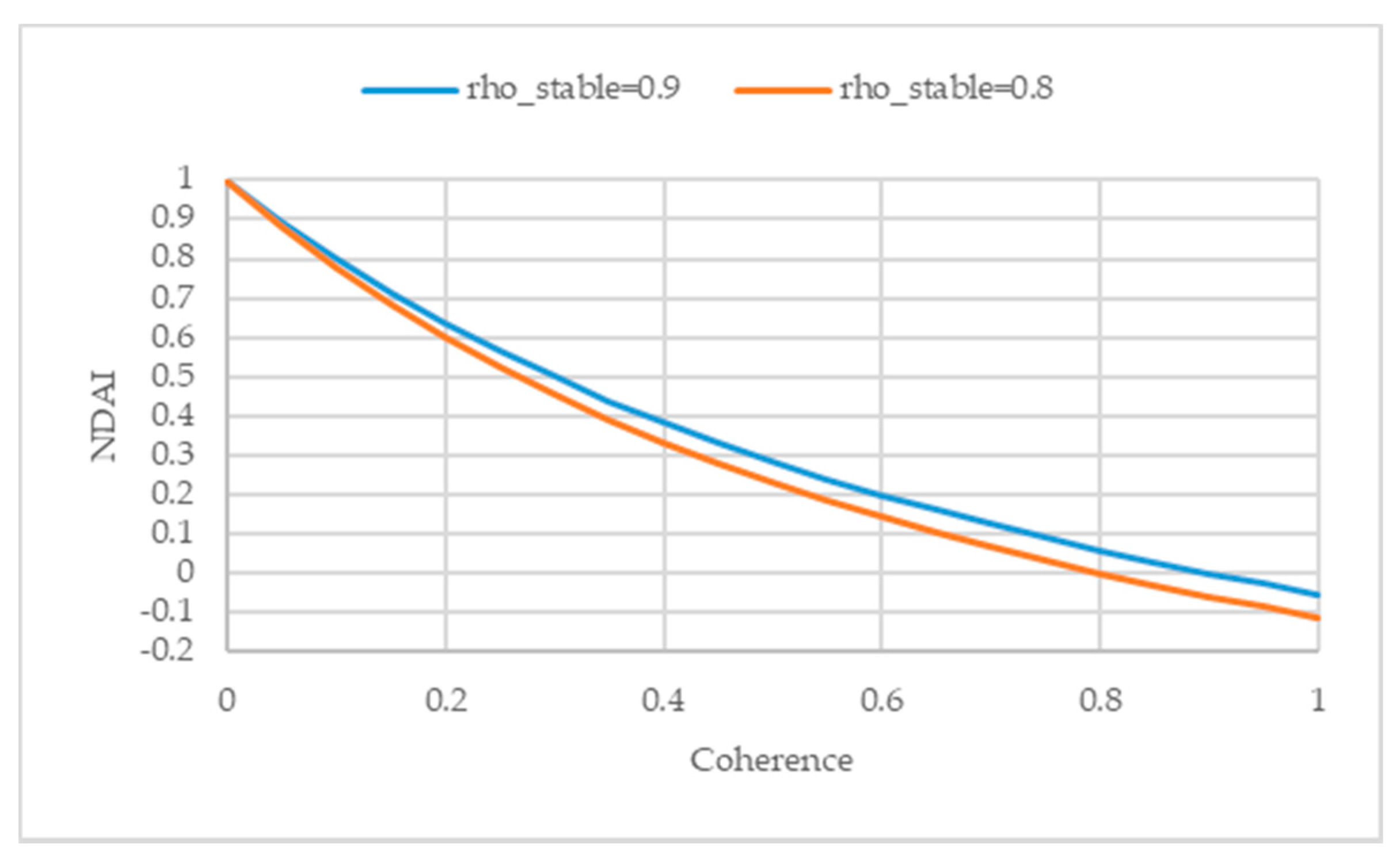
Being normalized, NDAI can have the value range of [−1, 1] numerically, but the actual lowest value is bounded, since . As shown in Figure 7, active targets with low coherence close to 0 will have NDAI close to 1, while targets with high coherence comparable to the selected stable points will be close to 0. Some man-made targets may have higher coherence than the selected stable points inside the mining area. In this case, NDAI may have negative values and can be interpreted as more stable targets than the selected natural stable points.
It is worth noting that was extracted inside the mining area (as depicted in the red polygon in Figure 5) to include natural targets only so that the and behave similarly. Otherwise, the noise response of man-made targets would be different from the mining area due to the double-bounce of buildings or building materials. The definition of mining area is performed based on the subtraction of DEMs, as described in the previous chapter and a series of historic Google Earth optical images.
2.3.4. Change Detection by RGB Composite of NDAIs
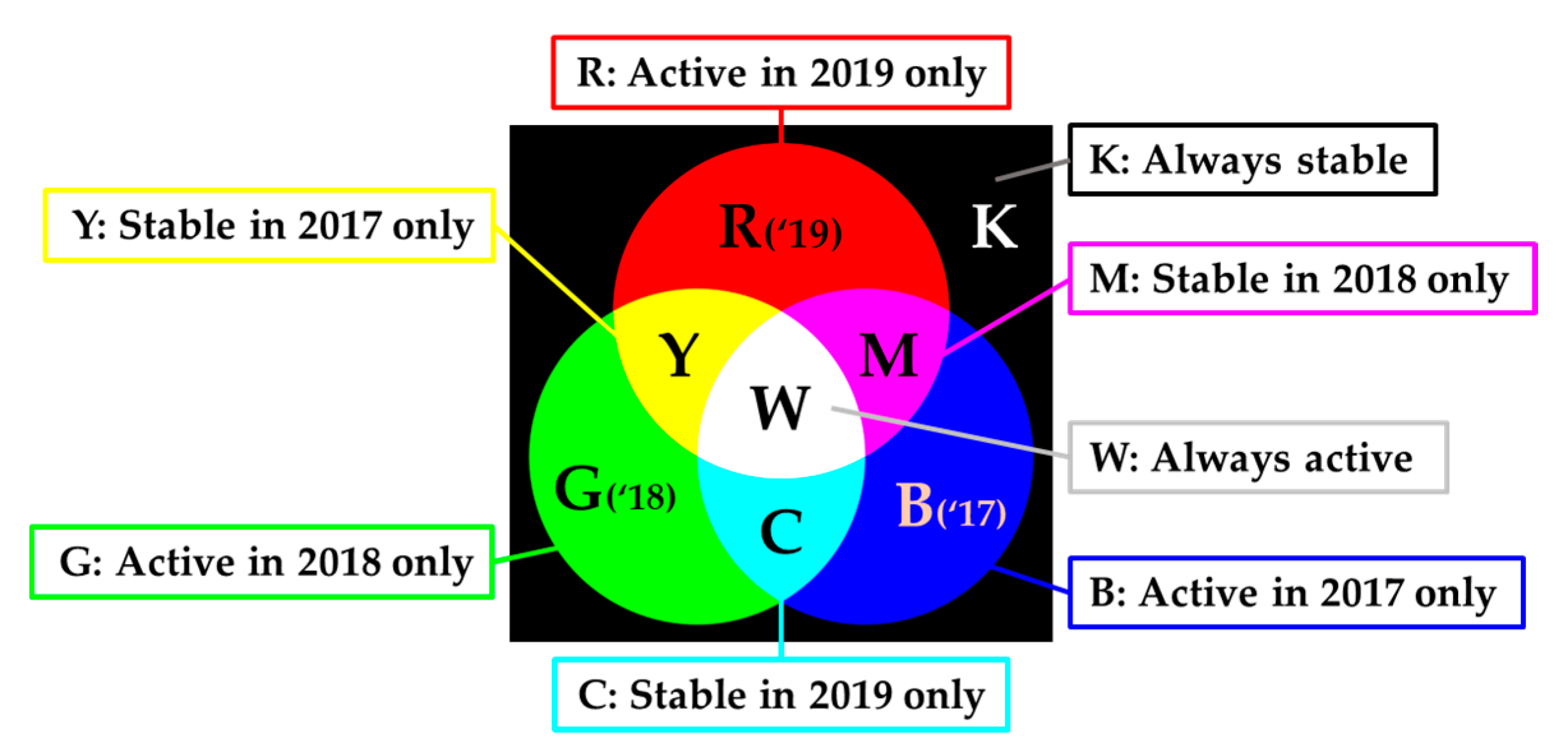
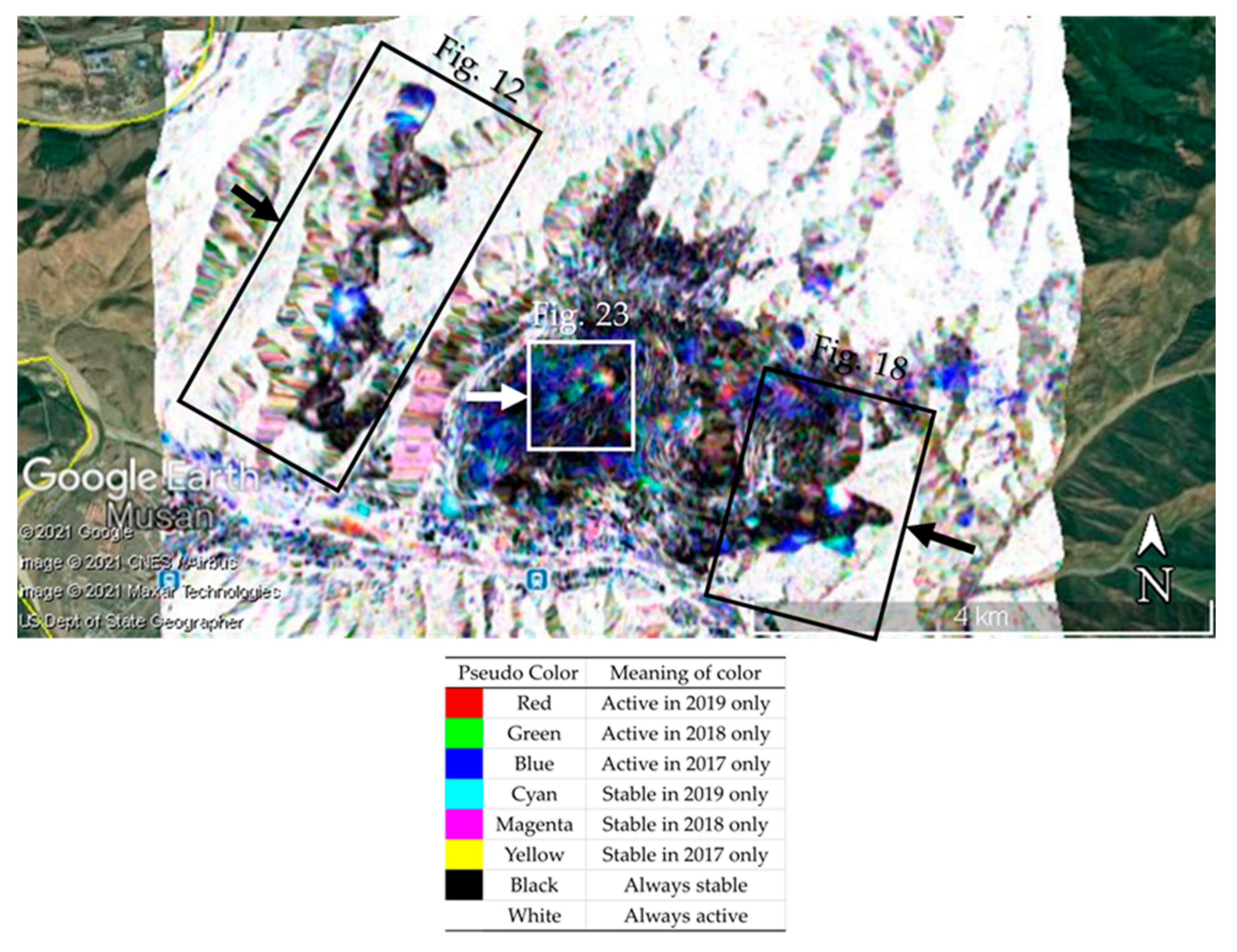
A pseudo-color image by an RGB composite of NDAI images can be generated to highlight the surface change due to mining activity (Figure 3). NDAI images for RGB channels can be averaged to represent activities over a certain period of time. In this study, NDAI maps over a year were averaged and used as an input to each RGB channels: R-channel for 2019, G-channel for 2018, and B-channel for 2017. RGB channels were linearly stretched to have Gaussian distribution for display. Figure 8 and Table 1 represent a pseudo-color scheme for this RGB composite image and the meaning of each color. For example, the red color (R) represents that the surface area was stable during 2017–2018 but became active in 2019. This could be the case if an excavation or accumulation site had been newly developed or expanded to this area recently in 2019. Similarly, the green color (G) tells us that the surface was active only for a year in 2018 and was stable before (2017) and after (2019). This could be the case where mining activity occurred within a year that started and finished in 2018 only. The blue color (B) means that the mining activity finished in 2017 and became stable afterward. Cyan (C), magenta (M), and yellow (Y) colors represent that the area was stable only in 2019, 2018, and 2017, respectively. Those three colors tell us that the surface was active for two years continuously, C (2017–2018) and Y (2018–2019), or sporadically active in 2017 and 2019 with a stable in the middle (2018). Black (K) means the area was always stable, while white color (W) represents that the area was active all the time for three years. Based on this RGB composite, the surface area can be categorized roughly by yearly based activities. A more detailed activity trend can also be investigated by using time-series NDVI graphs with a 12-day interval, from 2015 to 2020. Note that one can change the averaging period or temporal direction for RGB channels at the users’ discretion.
3. Results
3.1. InSAR DEM Change (2000–2015)
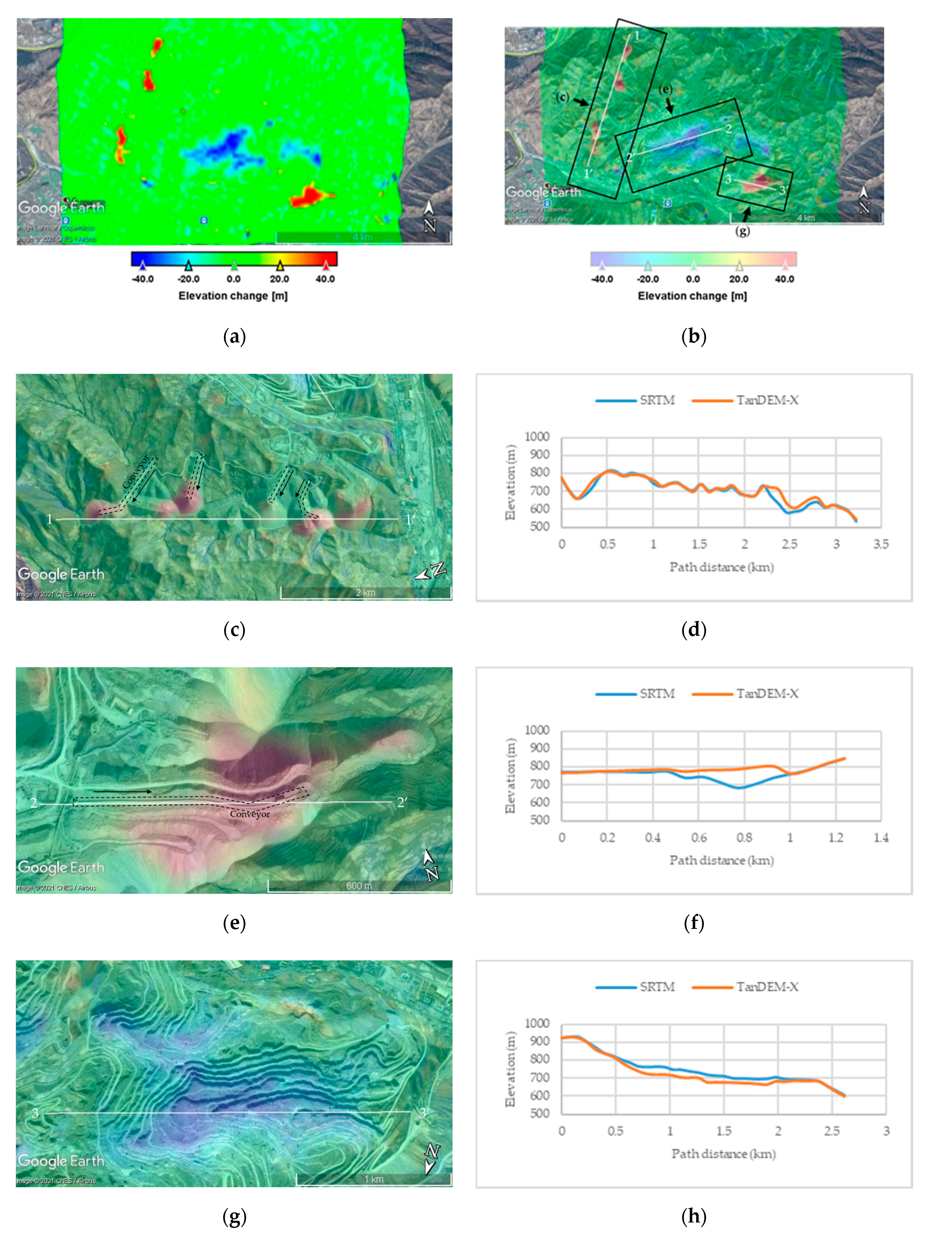
Figure 9a shows the change in elevation over Musan open-pit mine by subtracting SRTM DEM (2000) from TanDEM-X DEM (2010–2015). Major dumping areas were found in the east and the west of Musan mine (red color), while excavation sites were in the center (blue color). Maximum elevation changes and the size of the affected area were calculated in areas where elevation change exceeds 10 m. The dumping area located on the west side of the mine has a maximum elevation increase of about 84.0 m and the affected area of about 0.53 km2. For the dumping area in the east, the elevation increased up to 112.3 m, and the affected area was about 0.38 km2. The excavation site showed a maximum decrease in elevation of 42.5 m, and the affected area was about 1.82 km2.
Profiles of both DEMs were drawn for the dumping areas and excavation site, as shown in Figure 9b to check the elevation change in more detail. For 1-1′ in the west dumping area, a large amount of elevation increased at the tips of the conveyor belt lines, as shown in Figure 9c. The trend of elevation change along the slope shows a typical valley-fill dumping site, as shown in Figure 9d. For 2-2′ in the east dumping area, it was possible to confirm the expansion of the flat accumulation surface as the extension of the conveyor belt for dumping and also the valley-fill shape along the far east slope (Figure 9e,f). Figure 9g,h shows the excavation site (3-3′) with a concave-shaped open-pit mine. The elevation change was relatively uniform over the excavation site where drilling, blasting, and loading activities were performed along the benches step by step.
3.2. Averaged NDAI Map (2015–2020)
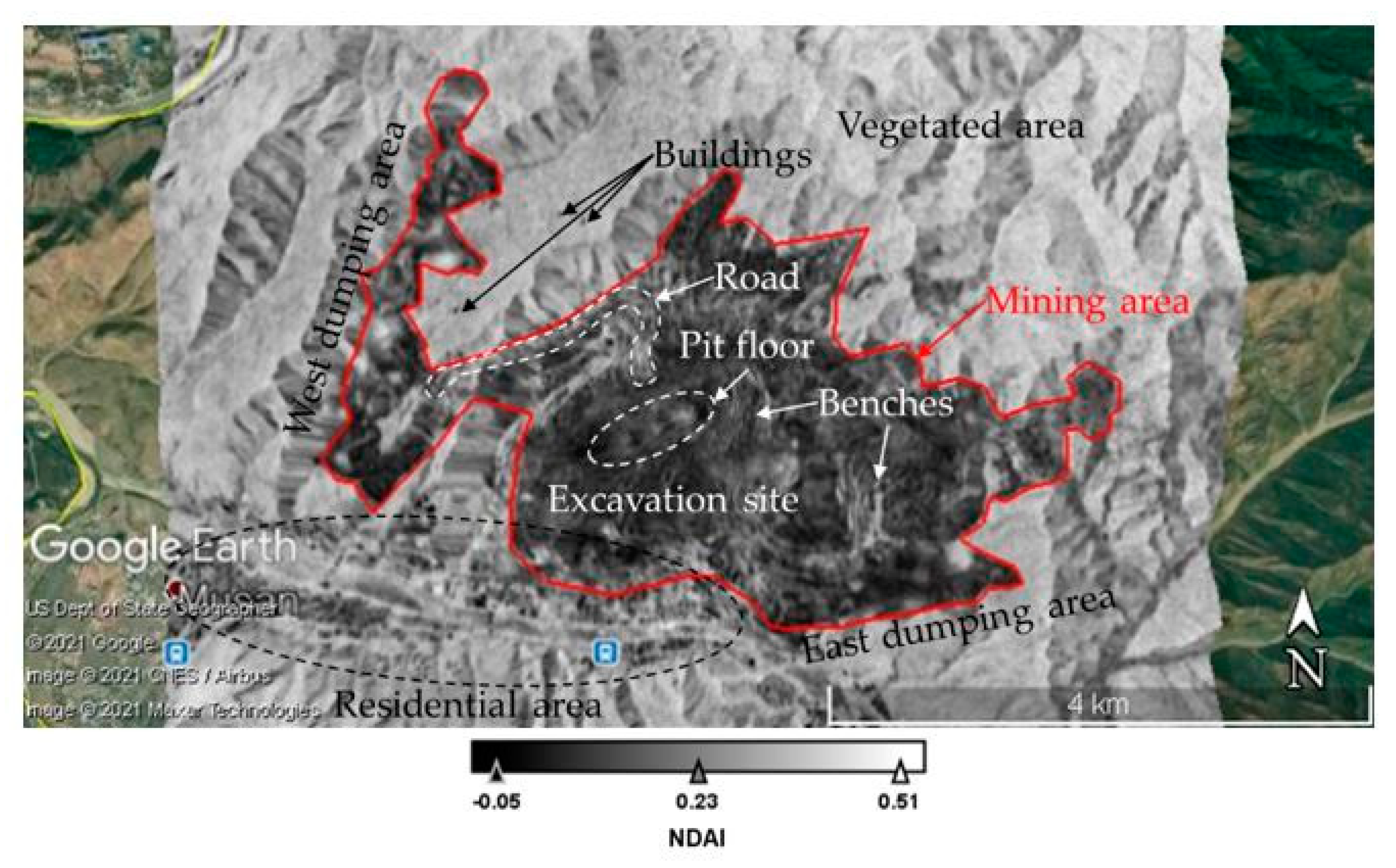
A total of 89 NDAI images obtained from Sentinel-1 A/B InSAR coherence images were averaged to see the overall mining activities of Musan mine from 2015 to early 2020. The averaged NDAI of a mining area is relatively low when compared with the surrounding area heavily covered with vegetation (Figure 10). Vegetated area is active in terms of InSAR phase statistics due to volume scattering and the effect of constantly wind-blown leaves and branches, resulting in a high NDAI all the time. On the other hand, the surface of the mining area is generally covered with bare rock; thus, it is stable and has low NDAI values unless mining activities are in progress. Stable black spots with negative NDAI values are also identified among the heavily vegetated areas. Those are the buildings that can be more stable than the natural stable targets selected for NDAI generation (Figure 10). There are also many man-made stable features with negative NDAI values in the residential area in the south of the mine. In the excavation area located in the center of the image, the shape of the benches can be clearly identifiable as high NDAI. This is due to the surface disturbance by the trucks moving on top of the bench. Clusters of high NDAI values inside the mining area, especially at the pit floor, are prominent over the stable rock surface, indicating active mining. The road from the excavation site to the dumping area can also be found in the average image. As the trucks move, wheel marks disturb the ground soil resulting in a high NDAI value. When waste rock is dumped along the slope, the NDAI value appears high from the top to the bottom of the dumping area. The dumping areas at Musan mine are mostly of valley-fill type where activity spreads from the top to the bottom of the valley, which will be shown in more detail in the next sections.
3.3. RGB Composite of Annually Averaged NDAI Maps (R: 2019, G: 2018, and B: 2017)
Figure 11 shows a pseudo-color image with RGB composite of the annually averaged NDAI maps: R for 2019, G for 2018, and B for 2017. Blue pixels, representing active in 2017 only and inactive afterward, are widely distributed throughout the mining area. This might be an important clue of the reduction in ore production due to the international sanctions imposed on North Korea after the 6th nuclear test on 3 September 2017. Cyan pixels (active in 2017 and 2018, and inactive in 2019) and green pixels (active in 2018 only) are also distributed at similar locations next to blue pixels, which can be interpreted as mining activity that has gradually shifted to nearby locations. Yellow, magenta, and red pixels indicating recent activities until 2019 occupy a relatively small area and are distributed sporadically. Clusters of white pixels are located in the center of the dumping area, and there are various colors around it. This means that the waste rock dumping slope has changed little by little on a yearly basis.
In the following sub-sections, the change in active area from 2017 to 2019 will be described in more detail for the dumping area in the west and the east, and for the excavation site in the center of Musan mine. Optical satellite images from Google Earth observed at different times will be shown to verify the surface changes if any. A time series NDAI graph for some points was also shown to determine the exact time of the activity change.
3.3.1. West Dumping Area
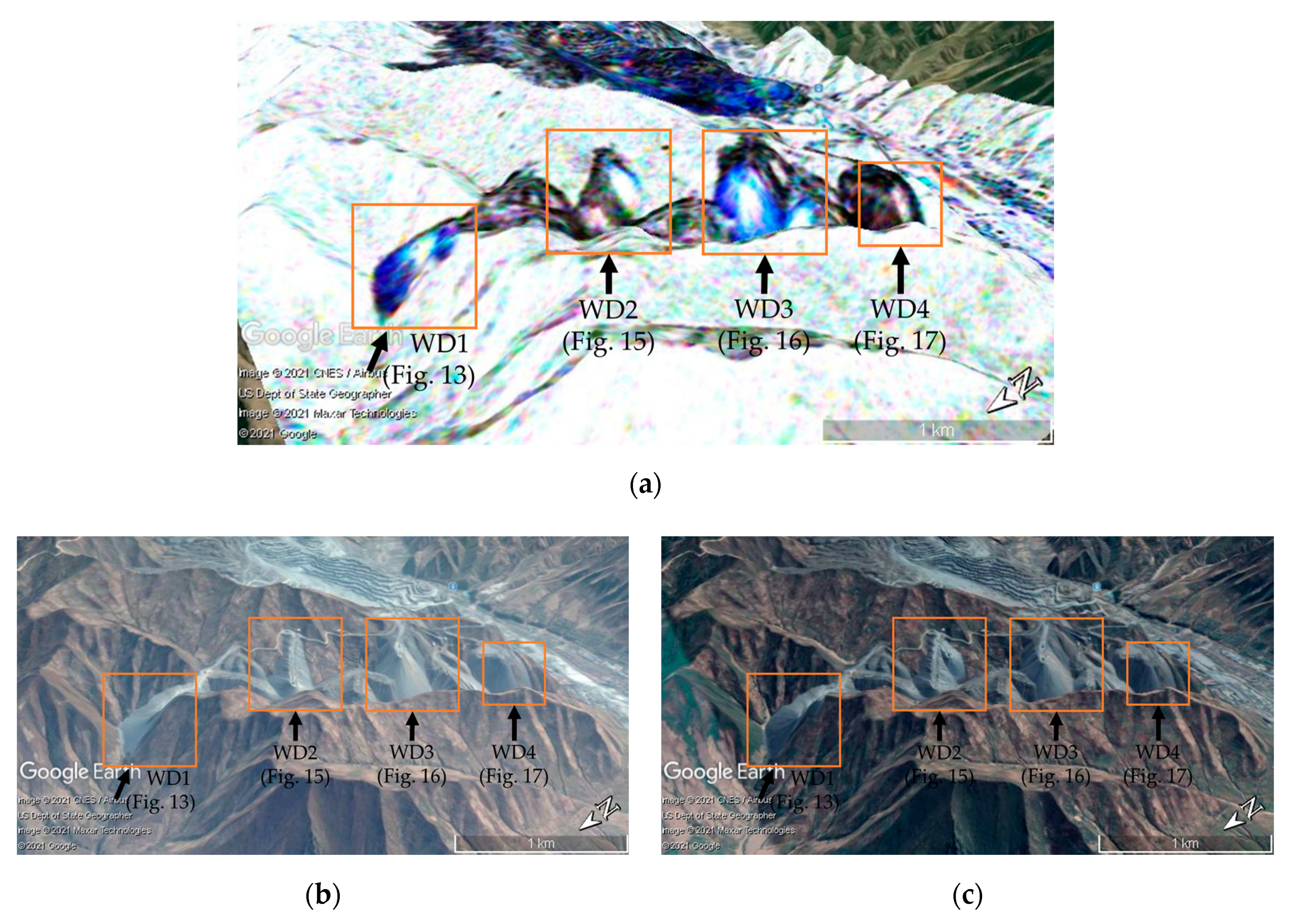
In the west dumping area located in the west-end of the mine, there are four major dumping sites that were active during 2017 to 2019, named West Dumping Site 1 (WD1), WD2, WD3, and WD4 in Figure 12a. Google Earth optical images obtained in 2015 and 2019 (Figure 12b,c) show the expansion of the dumping slopes in some areas. Google Earth provides other optical images taken from 2015 to 2019, but the image quality was not good enough due to cloud cover or image distortion from different look directions.
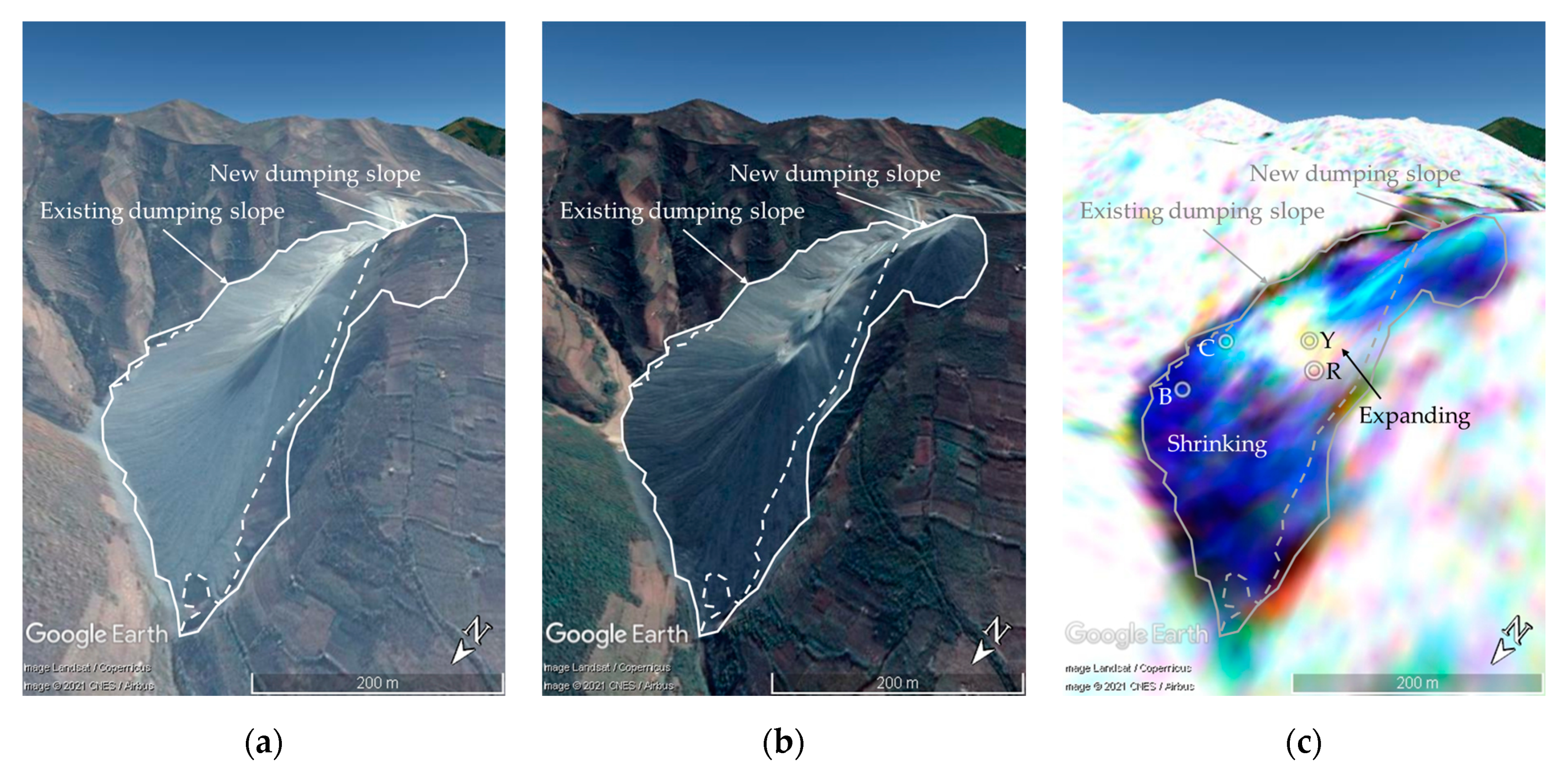
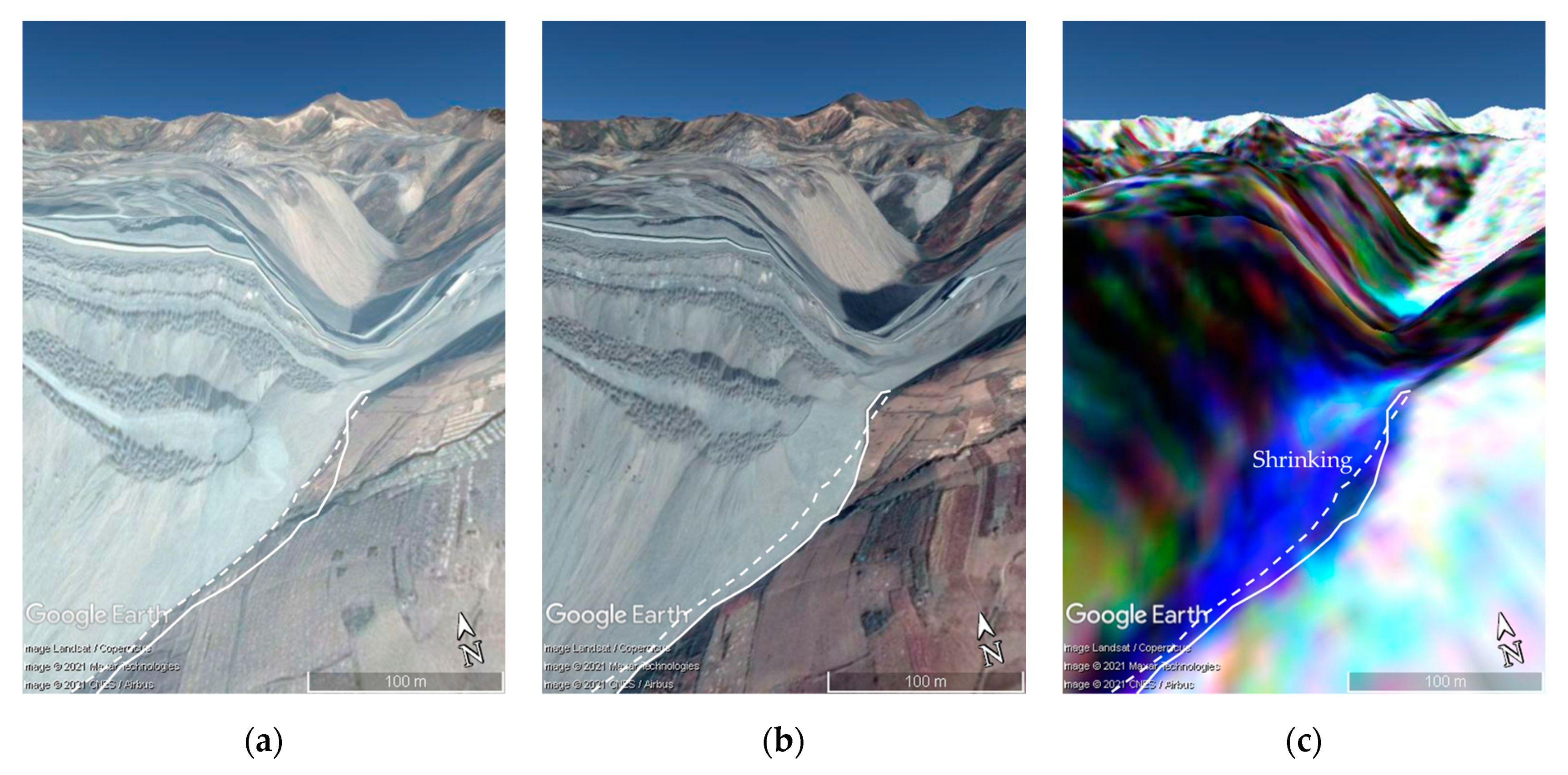
In general, different color patterns appear in the RGB composite of annually averaged NDAI between an expanding dumping slope and a shrinking dumping slope during 2017–2019. For an expanding dumping slope where the supply of dumping material is enough to expand the dumping area, the color changes from white (always active) at the top of the hill where dumping from the conveyor belt or trucks actually occurs, to yellow (active in 2018 and 2019 only) on the flank, and to red along the edges of the slope where the dumping area is newly expanded in 2019. In case of a shrinking dumping slope where dumping activity became reduced recently, color changes from white (always active) at the center where dumping activity still occurs, to cyan (active in 2017 and 2018 only) at the flank, and to blue (active in 2017 only) at the edge of the dumping slope. The latter case is dominant in the west dumping area in Musan mine, indicating overall reduction in ore production. More detailed analysis for those four major dumping sites are as follows.
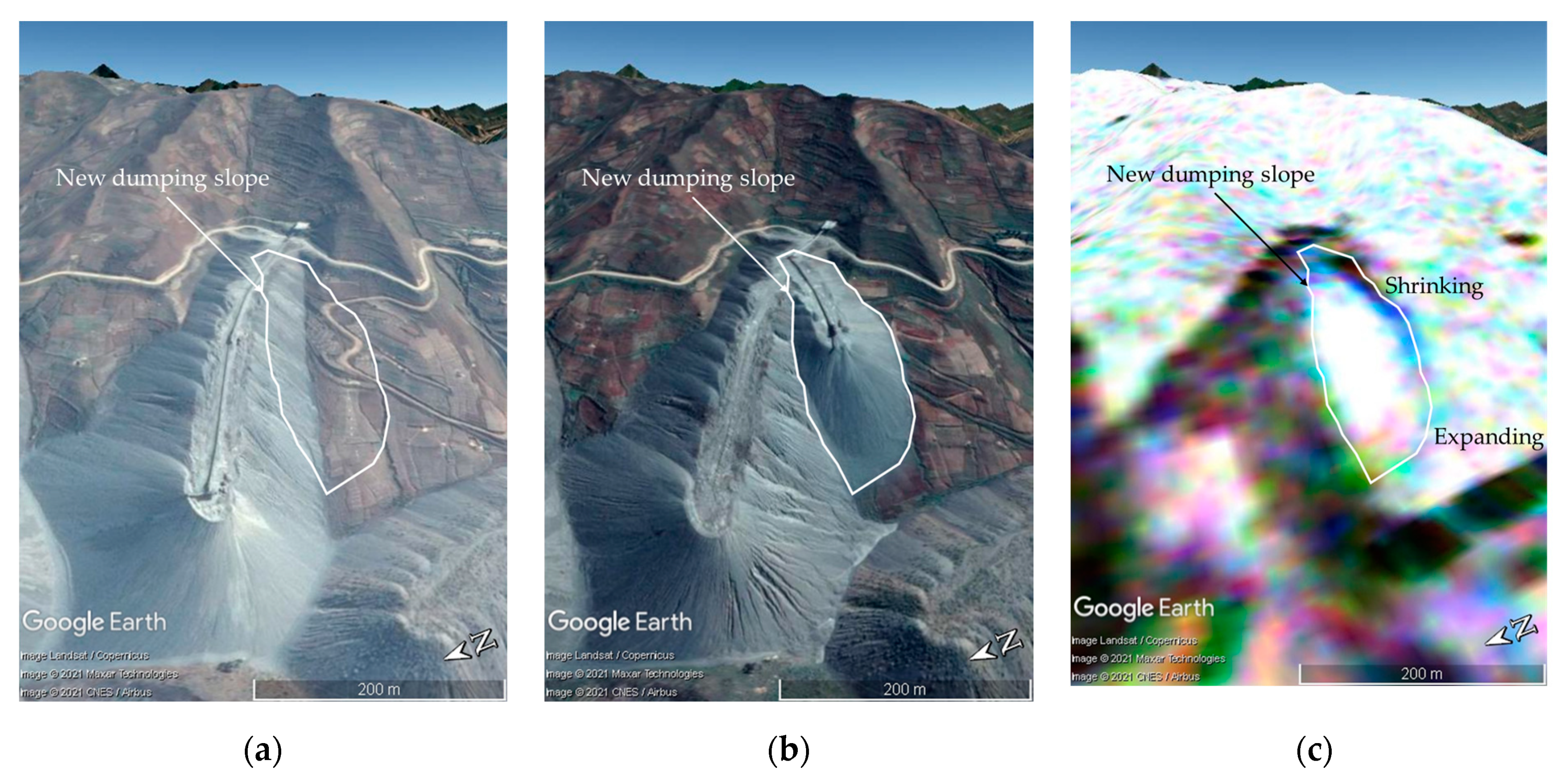
WD1 in Figure 13 shows both expanding and shrinking dumping slopes. A new dumping slope found in the upper right side of the Figure 13, by comparing the Google Earth images obtained in (a) 2015 and (b) 2019, respectively, has finished its main dumping activity between 2015–2017 and stabilized afterward, according to the RGB composite image of the annually averaged NDAI map (Figure 13c). This new dumping slope shows a shrinking pattern after 2018. In an existing dumping slope on the bottom left side, the color pattern changes from white at the top, cyan at the flank, and to blue at the edges of the slope, showing a typical shrinking dumping slope. However, this slope is partially expanding to the right side, showing white, yellow, and red pixels from the top to the bottom of the slope.
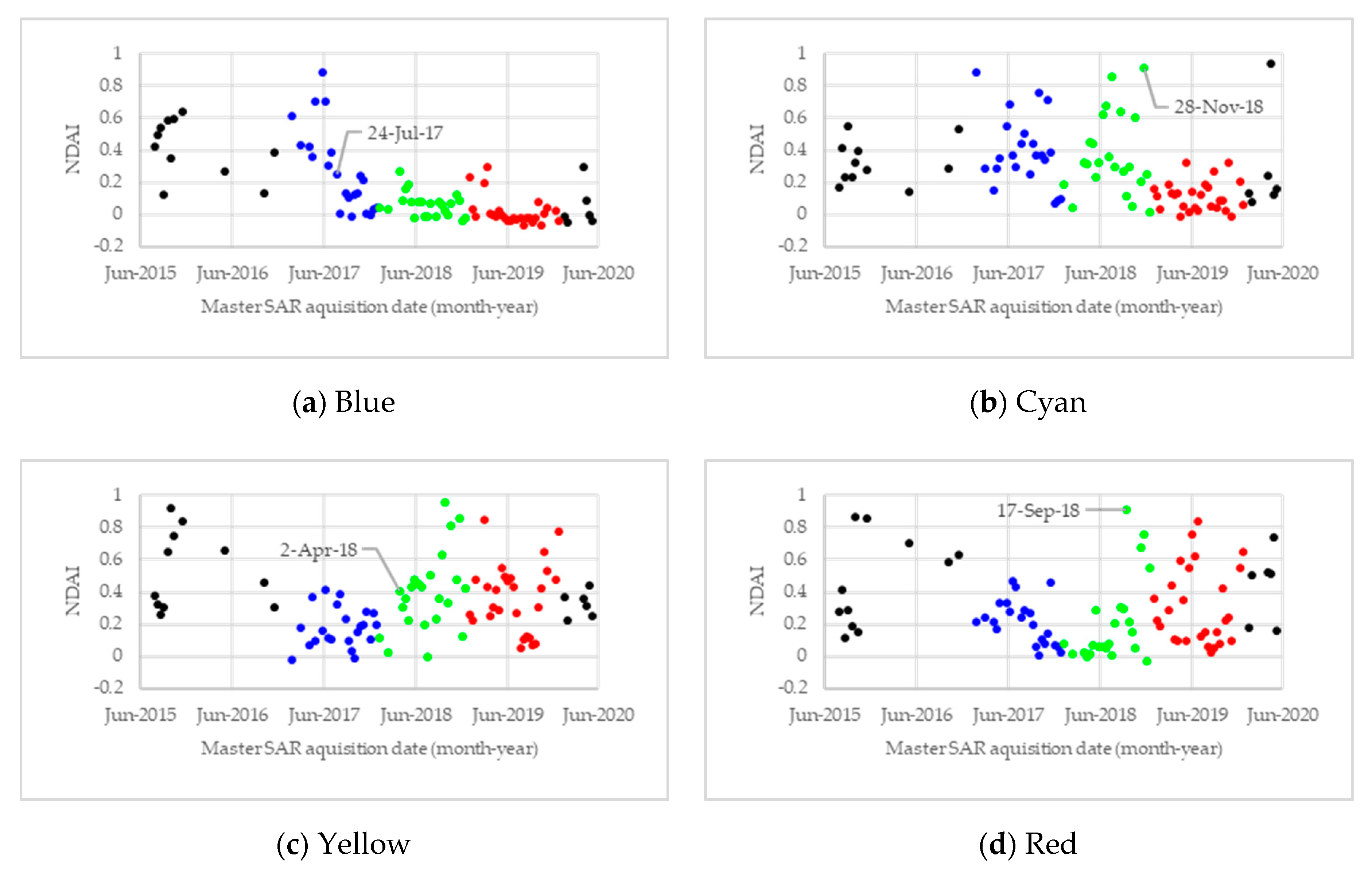
To check the activity in more detail at WD1, the NDAI graphs with 12-day intervals were extracted for some colors (Figure 14). In the NDAI graphs, each point represents the NDAI value calculated from the InSAR coherence image with a 12-day temporal baseline. The color of dots represents the data used for the RGB composite image of the annually averaged NDAI maps. Figure 14a shows that the blue color point (B) in Figure 13c was highly active from 2015 and suddenly reduced its activity after 24 July 2017. For the cyan color point (C), activity reduced after 28 November 2018 (Figure 14b). This indicates that the amount of the dumped waste rock reduced continuously and has not been enough to reach the bottom of the slope since July 2017. After November 2018, only the top area of the dumping slope shows activities that appear in white. The major expansion of the slope that happened is colored in yellow (Y) where activity began on 2 April 2018 (Figure 14c). A more recent expansion of the dumping slope appears in red (R) where activity started from 17 September 2018 and onward (Figure 14d).
WD2 also shows new expansions of a dumping slope that did not exist in the 2015 optical image in Figure 15a and appeared in 2019 in Figure 15b, as shown in a polygon. The shape of the new dumping slope has already formed in 2017, according to Figure 15c. The upper-right side of the slope has been stabilized since 2017 and shows a color pattern of a shrinking dumping slope, while the bottom of the slope shows a characteristic color pattern of an expanding dumping slope since 2018. The bottom left slope has also been active and expanding until recently, showing white to red from the top to the bottom of the slope.
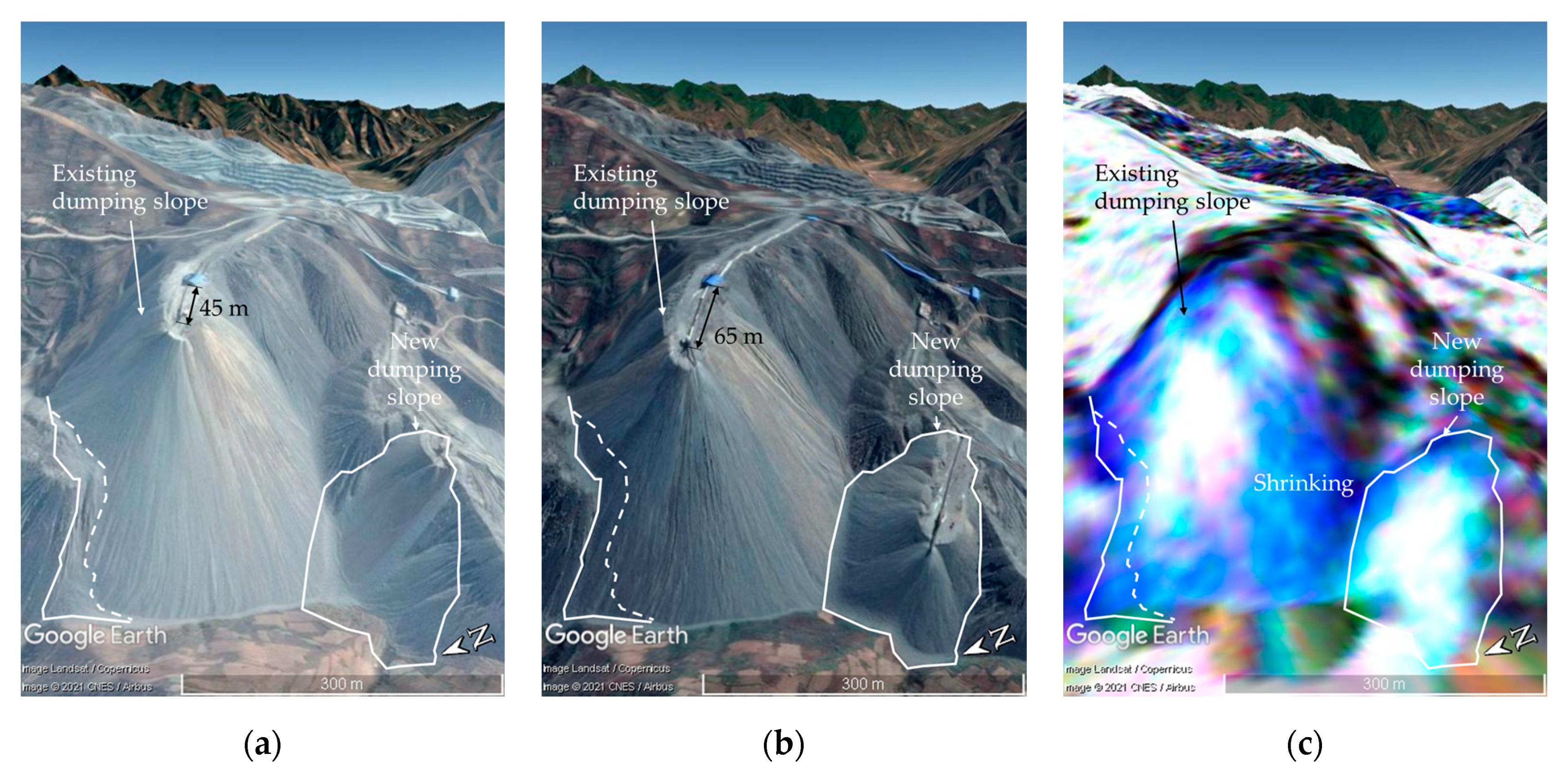
WD3 also shows the reduction in activity in the two dumping slopes after 2017 (Figure 16). A comparison of the optical images taken in 2015 and 2019 shows the expansion of the length of the conveyor belt in the existing dump site from about 45 to 65 m (Figure 16a,b). A new dumping slope appears in 2019 on the right side of the image. However, the major dumping activities finished in 2017, and the edge of the slopes remains stable after 2018 due to the reduced dumping activity (Figure 16c).
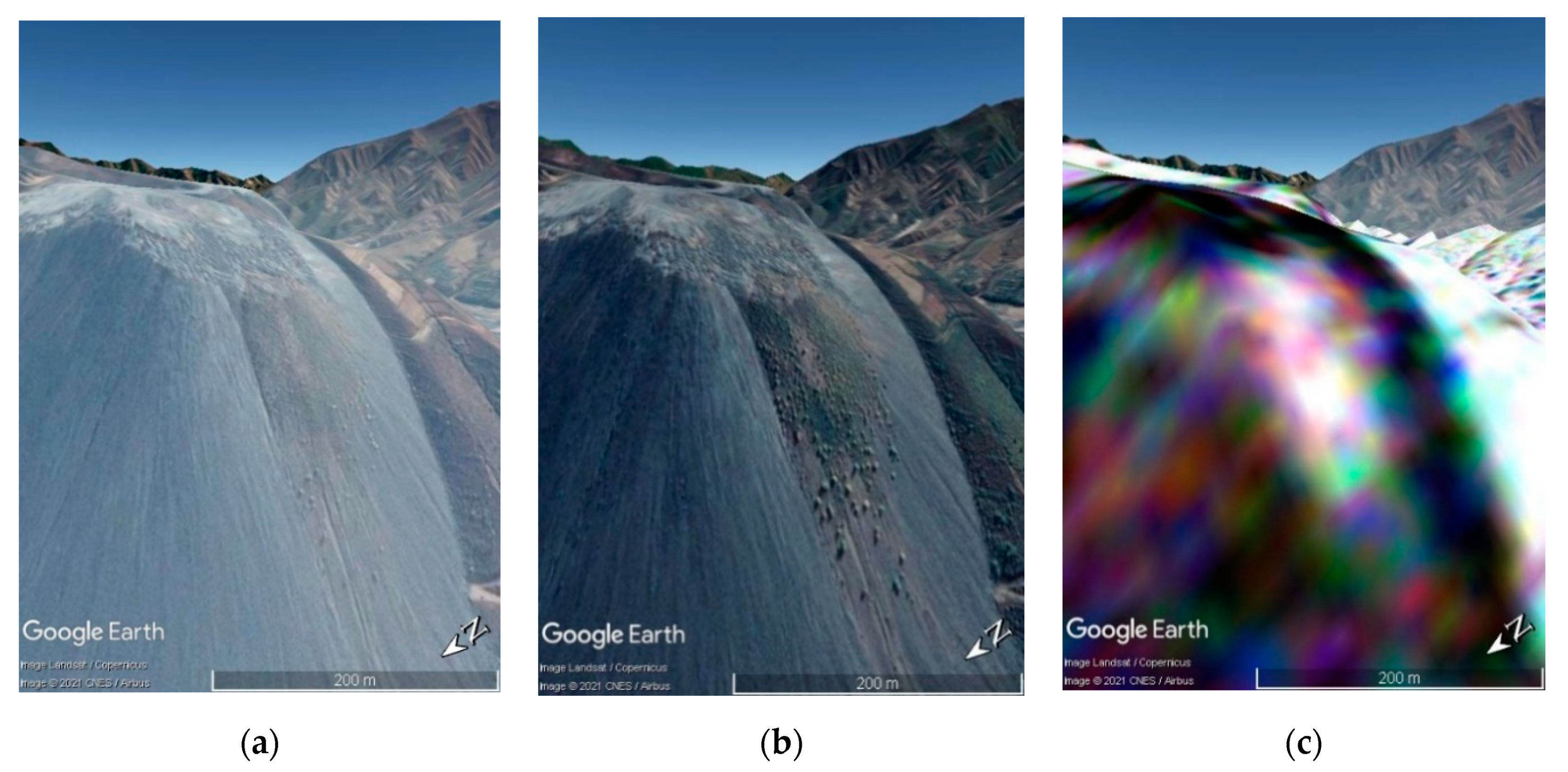
WD4 is an old dumping site where there is little change between 2015 and 2019, as shown on Google Earth images in Figure 17a,b. However, NDAI has a high value in the middle of the slope, as shown in Figure 17c, where sparse vegetation exists. Constant motion of sparse vegetation is causing low coherence on the slope and, thus, high NDAI all the time. Caution is required not to misinterpret it as a resumption of mining activity in this abandoned dumping slope.
In summary, the color pattern of the dumping slopes in WD1, WD2, and WD3 shows the shrinking dumping slope—white, cyan to blue from the top to the bottom of the slope—which indicates that the west dumping area of Musan mine was active until 2017 but reduced afterward.
3.3.2. East Dumping Area
There is another large dumping area in the east of the mine, where relatively active dumping had been progressing until recently. Three dumping slopes, named East Dumping Site 1 (ED1), ED2, and ED3 in Figure 18 are investigated further as below.
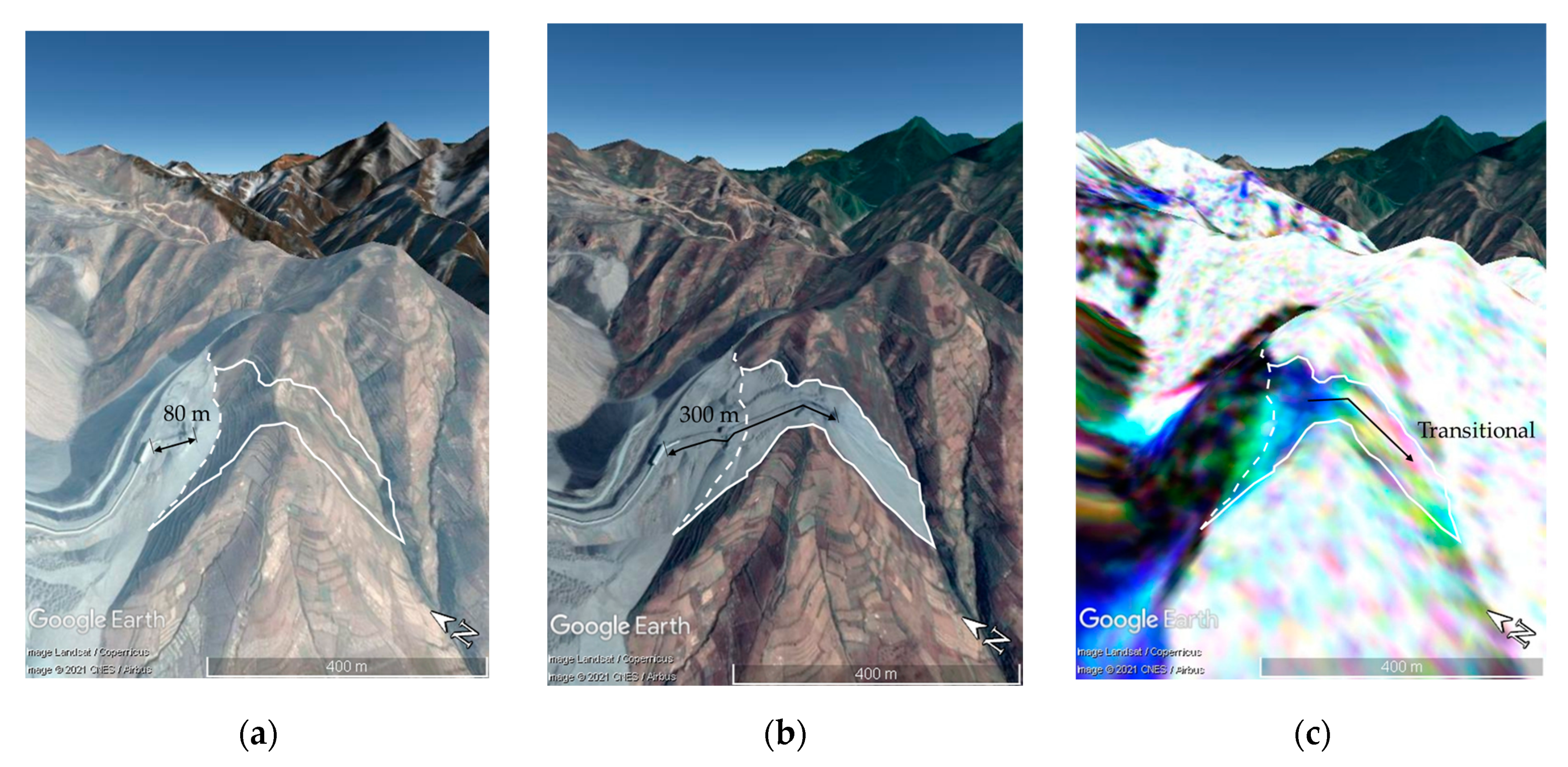
In an active area named as East Dumping Site 1 (ED1), Google Earth images show that there was a new dumping site in 2019 (Figure 19b,c). In Figure 19c, various color pixels appear around a cluster of white pixels. The color starts from blue in the upper part of the image to cyan in the flank, and to white at the top. The color continues to change from the top to the bottom of the slope in the lower image side of the image as from white, magenta, yellow, and to red at the bottom of the dumping slope (Figure 19c). The dumping progressed from the blue to white and magenta pixels until 2017, and the yellow area until 2018, and the red pixels in 2019. In this slope, dumping activity moves from one side to another, showing a shrinking color pattern on one side and an expanding one on the other side of the slope. One can call it a transitional dumping slope, apart from the previously defined shrinking or expanding dumping slope.
The 12-day NDAI graphs were examined at some locations of ED1 colored with blue (B), cyan (C), white (W), magenta (M), yellow (Y), and red (R) in Figure 19c. For B, the activity has been continuously high since 3 September 2015 until 3 December 2017, as shown in Figure 20a. For C, the activity started on 30 April 2016 and continued until 16 November 2019, as shown in Figure 20b, indicating the sequential expansion of this dumping slope. Once the active dumping slope had expanded and moved to a nearby location, then the old site became very stable afterward. The W point was stable and then became active after 9 October 2016 (Figure 20c). M was active in 2015 and 2017, then temporally inactive for a year in 2018, then resumed activity after 28 November 2018 (Figure 20d). The region Y maintains relatively high NDAI values over the entire period and became more active after 26 April 2018, as shown in Figure 20e. The high activity of the region M and Y before 2017 is because this area was covered with vegetation before dumping occurred. In the point R, new dumping activity started from 15 January 2019 over an old dumping slope that finished on 14 November 2015, as shown in Figure 20f.
Google Earth images of ED2 show the expansion of this dumping site sometime between 2015 and 2019, as shown in (Figure 21a,b). An RGB composite of the annually averaged NDAI map shows mostly blue and cyan on the slope, as shown in Figure 21c, which indicates that this dumping slope became inactive after 2018 and onward. The actual expansion identified by the Google Earth images had finished no later than 2017, and no further expansion occurred afterward.
In ED3, the conveyor belt had been expanded from 80 m in 2015 to 300 m in 2019, based on the Google Earth images (Figure 22a,b). Figure 22c shows that the activity near the boundary of ED3 in 2015 has been reduced to show blue to cyan pixels. However, the new valley-fill dumping site had been expanding until recently to show the change in colors from yellow to red along the expanding slope. Note that the DEM used in Google Earth does not represent recent elevation change in the dumping slope, resulting in unnatural topography of the dumping slope.
3.3.3. Excavation Site
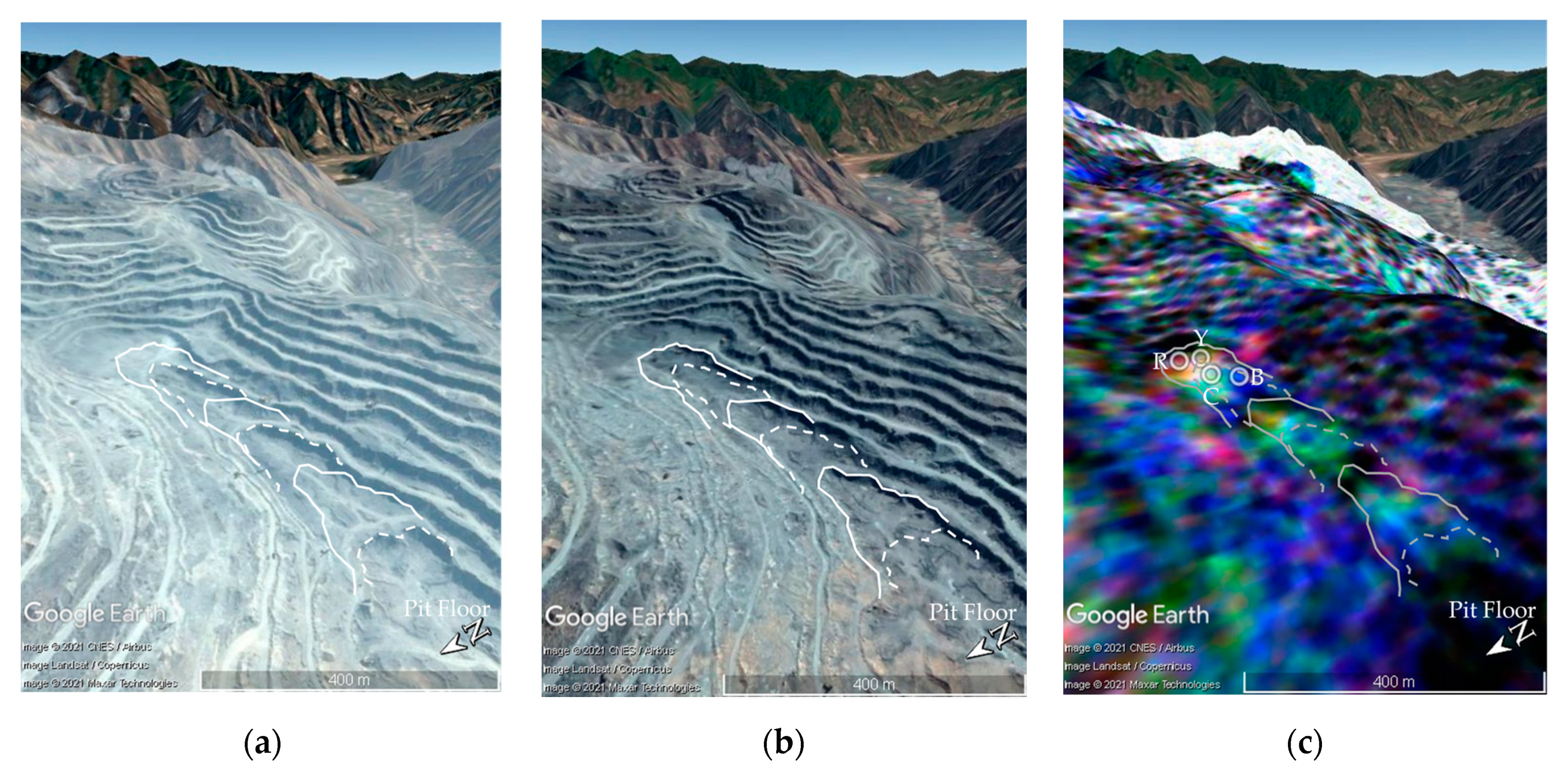
The major excavation site exists in the middle of Musan mine, where the topographic depression is prominent with many steps of benches. Google Earth images from 2015 and 2019 show the expansion of the pit floor and the change in shape at the bottom benches, as shown in Figure 23a,b. The excavation site is relatively stable, as shown in black color in the RGB composite of the annually averaged NDVI maps in Figure 23c except for the area near the pit floor. The main activities are shown at the bottom of the excavation site. Differently from the dumping areas, there are almost no large cluster of white pixels in the excavation area. This is because open-pit mines are developed in a way with balanced activities along the benches to prevent landslide. When benches are expanding near the pit floor, the activity appears in the form of an arc. A large portion of the area near the pit floor is blue, as shown in Figure 23c, indicating that major excavation activities along the benches occurred in 2017 only and stabilized afterward. Only the recent activities after 2018 happened on the bottom of the benches with the lowest altitude. Three benches were identified active recently near the pit floor. These benches expanded from the dashed line in 2015 to the solid line in 2019, as shown in Figure 23. Among them, the deepest bench (bottom right of the image) showed the largest expansion from 2015 to 2019. Color changes from B to R along the expansion direction, as shown in Figure 23c. Among three benches, the outmost bench shows a large variety of colors, indicating a rapidly expanding bench during 2017–2019.
The 12-day NDAI graphs of this bench in Figure 24a show that the color point B of Figure 23c was active in 2017 only and became stable afterward. The bench was then expanded to the point C (Figure 24b), Y (Figure 24c), and finally, to R (Figure 24d) in 2019. It was difficult to specify the exact dates of the onset and final days of activity from the 12-day NDAI graphs, because the excavation area is narrower than the dumping sites, and the activities are much more complex as a mixture of excavation and transportation. However, the rise and fall of the year-long activities can be identified by those 12-day NDAI graphs in Figure 24.
4. Discussion
The proposed NDAI is inversely proportional to coherence, as shown in Equation (5) and Figure 7. It is an advantage of NDAI that the values are proportional to the degree of surface activity, while coherence is a function of surface stability. The convenience appears when the major interest of user is the “activity” rather than “stability”. In this way, RGB composite images can be interpreted as the composite of activity indices at different times.
Another advantage of NDAI is the use of stable points as a reference to overcome temporal and spatial decorrelation beside the decorrelation from mining activity. NDAI makes use of the stable points statistically found by the time-averaged coherence and its standard deviation to assess the quality of the coherence image and mitigate the noise. The contribution of the stable points of NDAI includes two parts: One is the exclusion of the low coherence images heavily affected by snow or rainfall by using statistics from the stable targets. This is the process to mitigate by excluding images with 0.8 criterion, as shown in Figure 6a. The other is the reduction in the spatial baseline effect by calculating NDAI in Equation (3) so that a pixel having a coherence value of stable points () would have an NDAI value of 0 and can be declared absolutely stable similar to a coherence of 1.
To mitigate the noise of coherence from precipitation or spatial baseline using NDAI, we assumed that and are irrespective of target properties so that to derive Equation (5). It is worth noting that this assumption is correct provided that: (1) the targets are close enough with each other to be affected by the same weather and precipitation conditions; (2) the targets lay on flat area or on similar local slope, since geometrical decorrelation depends on both baseline and local slope; (3) the targets show the same scattering mechanisms (e.g., both are distributed scatterers). The diameter of Musan open-pit mine is 4 km with an area of 15 km2. The weather condition is thought to be homogeneous over the entire mine. However, possible errors from the difference of local slope or scattering mechanisms still remain. We expect that those errors have been mitigated to some degree by averaging the coherence of the stable points distributed widely throughout the mine. Foreshortening or layovers of an SAR image can be excluded by using local incidence angle, but the errors remain where elevation and slope changes due to mining activity.
It is difficult to set a quantitative criterion for the start or cease of the mining activity in the NDAI graphs. There is no specific NDAI criterion for activation/deactivation of the mining in this study. The onset of mining activities was interpreted with relative NDAI values or general trend in temporal graphs or spatial maps. Similar uncertainty occurs in other indices such as the conventional coherence and normalized difference vegetation index (NDVI), where no specific value can act as a criterion for image classification and segmentation. More analysis is necessary to determine the quantitative criterion, but it is dependent on location, situation, and time. The trend of NDVI depends on the characteristics of mining activities. For example, an abrupt increase in NDAI occurs near the edge of the expanding dumping slopes, while activity continues near the inlet of the shrinking dumping slopes. Some part of the excavation site would have preparatory activities such as vehicles on the road or drilling activities before the actual blasting and excavation. The stability of the surface also depends on the size of rocks, types of soil, or vegetation that cover the surface. NDAI value of less than 0.2 over the bare rock surface could be considered as stable empirically in this study. However, further analysis with sufficient collection of in situ data would be necessary to quantify the behavior of NDAI for each target surface.
Colors in RGB composites are useful to determine the spatial variations of mining activity, but the exact color varies image to image. Only the eight representative colors of R, G, B, C, M, Y, W, and K have been interpreted in this study, but more detailed colors can be explained. A reduction in noise by time averaging is also an advantage for the RGB composite of the annually averaged NDAI method. The RGB composite in this study is based on annual average only. However, the mining activity and the change are not necessarily annual-related. The annual averaging is just one effective way of representing time-series information. Seasonal or monthly averaging can be another way for some locations or events.
Regression of time-series NDAI data can be useful for the event with long-term variation. However, mining activities contain high-frequency information—they start suddenly and stop abruptly. Vegetated areas maintain high NDAI and are difficult to differentiate with mining activity. The regrowth of vegetation over the abandoned dumpsite might have been misinterpreted as a resumption of mining activity. This can be overcome by using historical high-resolution optical images of Google Earth, as shown in this paper.
5. Conclusions
By using InSAR DEMs and time-series of Sentinel-1A/B InSAR coherence images, it was possible to investigate the mining activity in the accumulation and excavation areas of Musan open-pit mine, North Korea, where field data could not be easily obtained. The change in InSAR DEM between SRTM in 2000 and TanDEM-X in 2010–2015 confirmed large elevation change in the major dumping areas in the west (+84.0 m) and the east (+112.3 m) and an excavation area (−42.5 m) in the center of the Musan mine. As a new activity indicator based on coherence image, NDAI was developed to cope with spatial and temporal (weather) decorrelation of the coherence images. Stable points were detected and analyzed for the generation of NDAI and to remove the coherence images severely degraded by a snow fall event in the winter time. The RGB composite of the annually averaged NDAI showed a yearly trend of mining activities. It was found that the overall mining activity was reduced significantly after 2017 probably due to the international sanctions imposed to North Korea due to the nuclear test on September 2017. By the change in color patterns, we could identify three types of dumping slopes such as expanding, shrinking, or transitional.
The proposed RGB composite scheme of averaged NDAI can be applied with a different averaging span for different temporal resolution of activity. The 12-day NDAI was successfully applied to determine the onset of accumulation and/or excavation process with monthly accuracy. The methods developed in this study can be applied to other open-pit mines. The continuous acquisition of Sentinel-1A/B SAR data would always be beneficial to the ongoing monitoring of mining activities in the remote and large area.
Author Contributions
Conceptualization, J.M. and H.L.; methodology, J.M. and H.L.; software, J.M. and H.L.; validation, J.M. and H.L.; formal analysis, J.M. and H.L.; investigation, J.M. and H.L.; resources, H.L.; data curation, J.M. and H.L.; writing—original draft preparation, J.M.; writing—review and editing, H.L.; visualization, J.M.; supervision, H.L.; project administration, H.L.; funding acquisition, H.L. All authors have read and agreed to the published version of the manuscript.
Funding
This research was funded by the Basic Research Project of Korea Institute of Geoscience and Mineral Resources (KIGAM) funded by the Ministry of Science and ICT of Korea and the National Research Foundation of Korea (NRF-2019R1F1A1041389 and No. 2019R1A6A1A03033167).
Institutional Review Board Statement
Not applicable.
Informed Consent Statement
Not applicable.
Data Availability Statement
The data presented in this study are available on request from the corresponding author.
Conflicts of Interest
The authors declare no conflict of interest.
References
- Yang, H.; Kang, S.; Seonwoo, C.; Jang, M.; Jeong, S.; Cho, S. Surface Mining Engineering; CIR: Seoul, Korea, 2016; pp. 5–292. [Google Scholar]
- Kobayashi, H.; Watando, H.; Kakimoto, M. A global extent site-level analysis of land cover and protected area overlap with mining activities as an indicator of biodiversity pressure. J. Clean. Prod. 2014, 84, 459–468. [Google Scholar] [CrossRef] [Green Version]
- Murguía, D.I.; Bringezu, S.; Schaldach, R. Global direct pressures on biodiversity by large-scale metal mining: Spatial distribution and implications for conservation. J. Environ. Manag. 2016, 180, 409–420. [Google Scholar] [CrossRef] [PubMed]
- Moreno-de Las Heras, M.; Merino-Martín, L.; Nicolau, J.M. Effect of vegetation cover on the hydrology of reclaimed mining soils under Mediterranean-Continental climate. Catena 2009, 77, 39–47. [Google Scholar] [CrossRef]
- Chen, W.T.; Li, X.J.; Wang, L.Z. Fine Land Cover Classification in an Open Pit Mining Area Using Optimized Support Vector Machine and WorldView-3 Imagery. Remote Sens. 2020, 12, 82. [Google Scholar] [CrossRef] [Green Version]
- Beighley, R.E.; Moglen, G.E. Trend assessment in rainfall-runoff behavior in urbanizing watersheds. J. Hydrol. Eng. 2002, 7, 27–34. [Google Scholar] [CrossRef]
- Simmons, J.A.; Currie, W.S.; Eshleman, K.N.; Kuers, K.; Monteleone, S.; Negley, T.L.; Pohland, B.R.; Thomas, C.L. Forest to reclaimed mine land use change leads to altered ecosystem structure and function. Ecol. Appl. 2008, 18, 104–118. [Google Scholar] [CrossRef]
- Townsend, P.A.; Helmers, D.P.; Kingdon, C.C.; McNeil, B.E.; de Beurs, K.M.; Eshleman, K.N. Changes in the extent of surface mining and reclamation in the Central Appalachians detected using a 1976–2006 Landsat time series. Remote Sens. Environ. 2009, 113, 62–72. [Google Scholar] [CrossRef]
- LaJeunesse Connette, K.J.; Connette, G.; Bernd, A.; Phyo, P.; Aung, K.H.; Tun, Y.L.; Thein, Z.M.; Horning, N.; Leimgruber, P.; Songer, M. Assessment of mining extent and expansion in Myanmar based on freely-available satellite imagery. Remote Sens. 2016, 8, 912. [Google Scholar] [CrossRef] [Green Version]
- Julzarika, A. Mining land identification in Wetar Island using remote sensing data. J. Degrad. Min. Lands Manag. 2018, 6, 1513–1518. [Google Scholar] [CrossRef]
- Lobo, F.D.L.; Souza-Filho, P.W.M.; Novo, E.M.L.d.M.; Carlos, F.M.; Barbosa, C.C.F. Mapping Mining Areas in the Brazilian Amazon Using MSI/Sentinel-2 Imagery (2017). Remote Sens. 2018, 10, 1178. [Google Scholar] [CrossRef] [Green Version]
- Ross, M.R.V.; McGlynn, B.L.; Bernhardt, E.S. Deep impact: Effects of mountaintop mining on surface topography, bedrock structure, and downstream waters. Environ. Sci. Technol. 2016, 50, 2064–2074. [Google Scholar] [CrossRef] [PubMed] [Green Version]
- Lee, H. Application of KOMPSAT-5 SAR Interferometry by using SNAP software. Korean J. Remote Sens. 2017, 33, 1215–1221. [Google Scholar]
- Farr, T.G.; Rosen, P.A.; Caro, E.; Crippen, R.; Duren, R.; Hensley, S.; Kobrick, M.; Paller, M.; Rodriguez, E.; Roth, L.; et al. The shuttle radar topography mission. Rev. Geophys. 2007, 45, RG2004. [Google Scholar] [CrossRef] [Green Version]
- Wu, Q.; Song, C.; Liu, K.; Ke, L. Integration of TanDEM-X and SRTM DEMs and Spectral Imagery to Improve the Large-Scale Detection of Opencast Mining Areas. Remote Sens. 2020, 12, 1451. [Google Scholar] [CrossRef]
- Wang, S.; Lu, X.; Chen, Z.; Zhang, G.; Ma, T.; Jia, P.; Li, B. Evaluating the feasibility of illegal open-pit mining identification using insar coherence. Remote Sens. 2020, 12, 367. [Google Scholar] [CrossRef] [Green Version]
- Cenni, N.; Fiaschi, S.; Fabris, M. Monitoring of Land Subsidence in the Po River Delta (Northern Italy) Using Geodetic Networks. Remote Sens. 2021, 13, 1488. [Google Scholar] [CrossRef]
- Iasio, C.; Novali, F.; Corsini, A.; Mulas, M.; Branzanti, M.; Benedetti, E.; Giannico, C.; Tamburini, A.; Mair, V. COSMO SkyMed high frequency—High resolution monitoring of an alpine slow landslide, corvara in Badia, Northern Italy. In Proceedings of the IEEE International Geoscience and Remote Sensing Symposium (IGARSS), Munich, Germany, 22–27 July 2012; pp. 7577–7580. [Google Scholar]
- Tarighat, F.; Foroughnia, F.; Perissin, D. Monitoring of Power Towers’ Movement Using Persistent Scatterer SAR Interferometry in South West of Tehran. Remote Sens. 2021, 13, 407. [Google Scholar] [CrossRef]
- Matikainen, L.; Lehtomäki, M.; Ahokas, E.; Hyyppä, J.; Karjalainen, M.; Jaakkola, A.; Kukko, A.; Heinonen, T. Remote sensing methods for power line corridor surveys. ISPRS J. Photogramm. Remote Sens. 2016, 119, 10–31. [Google Scholar] [CrossRef] [Green Version]
- Cando Jácome, M.; Martinez-Graña, A.M.; Valdés, V. Detection of Terrain Deformations Using InSAR Techniques in Relation to Results on Terrain Subsidence (Ciudad de Zaruma, Ecuador). Remote Sens. 2020, 12, 1598. [Google Scholar] [CrossRef]
- Lee, H. Investigation of SAR Systems, technologies and application fields by a statistical analysis of SAR-related journal papers. Korean J. Remote Sens. 2006, 22, 153–174. [Google Scholar]
- Khalil, R.Z.; Saad-ul-Haque. InSAR coherence-based land cover classification of Okara, Pakistan. Egypt. J. Remote Sens. Space Sci. 2018, 21, S23–S28. [Google Scholar] [CrossRef]
- Korean Statistical Information Service. Available online: https://kosis.kr/index/index.do (accessed on 10 February 2021).
- Choi, K. The Mining Industry of North Korea. Korean J. Defense Anal. 2011, 23, 211–230. [Google Scholar]
- Bae, S.; Yu, J.; Koh, S.M.; Heo, C.H. 3D Modeling Approaches in Estimation of Resource and Production of Musan Iron Mine, North Korea. Econ. Environ. Geol. 2015, 48, 391–400. [Google Scholar] [CrossRef] [Green Version]
- Koh, S.M.; Lee, G.J.; Yoon, E. Status of Mineral Resources and Mining Development in North Korea. Econ. Environ. Geol. 2013, 46, 291–300. [Google Scholar] [CrossRef] [Green Version]
- Kim, N.; Koh, S.M.; Lee, B.H. Geological Comparison Between Musan Iron Deposit in North Korea and Iron Deposits in Anshan-Benxi Area in China. J. Miner. Soc. Korea 2018, 31, 215–225. [Google Scholar] [CrossRef]
- Yoon, S.; Jang, H.; Yun, S.T.; Kim, D.M. Investigating the Status of Mine Hazards in North Korea Using Satellite Pictures. J. Korean Soc. Miner. Energy Resour. Eng. 2018, 55, 564–575. [Google Scholar] [CrossRef]
- Oh, M.; Yang, A.; Koo, Y.H.; Park, H.D. Assessment and comparison of landslide susceptibility at open-pit mines in North Korea using GIS. IOP Conf. Ser. Earth Environ. Sci. 2020, 509, 012041. [Google Scholar]
- Oh, M.; Son, J.; Park, H.D. Photovoltaic Energy Assessment near the Musan Iron Mine, North Korea, to Supply Energy. In Proceedings of the 2020 Annual Spring Meeting of the Korean Society for New & Renewable Energy, Seoul, Korea, 24–25 August 2020. [Google Scholar]
- Kim, S.M.; Suh, J.; Oh, M.; Yang, A.; Song, J.; Park, H.D. GIS-based Network Analysis of North Korea’s Transportation Infrastructure for the Trade of Mineral Resources in North Korea. J. Korean Soc. Miner. Energy Resour. Eng. 2020, 57, 159–167. [Google Scholar] [CrossRef]
- Park, J.; Joung, E. Study on North Koreas iron ore trade toward China: Focusing on the Development Situation of Musan mine. J. Northeast Asian Stud. 2017, 85, 73–98. [Google Scholar] [CrossRef]
- Kim, K.H. Reserves 5.2 billion ton(Fe 24%) of World-class open-pit mine: Clough Engineering Ltd. and Mitsui Mineral Development Engineering Co. Ltd. make a report together <First report about the present condition and investment opportunity of Musan Iron mine>. Minjog21 2002, 10, 108–113. [Google Scholar]
- Yoon, E. Status of Future of the North Korean Minerals Sector. Korean J. Defense Anal. 2011, 23, 191–210. [Google Scholar]
- Chung, J. The Mineral Industry of North Korea. Miner. Yearb. 2016, 3, 14.1–14.5. [Google Scholar]
- Nam, S.Y. Development of iron ore from North Korea and Inter-Korean Cooperation. Korean J. Unification Aff. 2014, 26, 75–113. [Google Scholar]
- Krieger, G.; Moreira, A.; Fiedler, H.; Hajnsek, I.; Werner, M.; Younis, M.; Zink, M. TanDEM-X: A satellite formation for high-resolution SAR interferometry. IEEE Trans. Geosci. Remote Sens. 2007, 45, 3317–3341. [Google Scholar] [CrossRef] [Green Version]
- Krieger, G.; Zink, M.; Bachmann, M.; Bräutigam, B.; Schulze, D.; Martone, M.; Rizzoli, P.; Steinbrecher, U.; Walter Antony, J.; de Zan, F.; et al. TanDEM-X: A radar interferometer with two formation-flying satellites. Acta Astronaut. 2013, 89, 83–98. [Google Scholar] [CrossRef] [Green Version]
- Zink, M.; Bachmann, M.; Bräutigam, B.; Fritz, T.; Hajnsek, I.; Krieger, G.; Moreira, A.; Wessel, B. TanDEM-X: The New Global DEM Takes Shape. IEEE GRSM 2014, 2, 8–23. [Google Scholar] [CrossRef]
- Rizzoli, P.; Martone, M.; Gonzalez, C.; Wecklich, C.; Tridon, D.B.; Bräutigam, B.; Bachmann, M.; Schulze, D.; Fritz, T.; Huber, M.; et al. Generation and performance assessment of the global TanDEM-X digital elevation model. ISPRS J. Photogramm. Remote Sens. 2017, 132, 119–139. [Google Scholar] [CrossRef] [Green Version]
- Geudtner, D.; Torres, R.; Snoeij, P.; Davidson, M.; Rommen, B. Sentinel-1 system capabilities and applications. In Proceedings of the 2014 IEEE International Geoscience and Remote Sensing Symposium (IGARSS), Quebec City, QC, Canada, 13–18 July 2014; pp. 1457–1460. [Google Scholar]
- Torres, R.; Snoeij, P.; Geudtner, D.; Bibby, D.; Davidson, M.; Attema, E.; Potin, P.; Rommen, B.; Floury, N.; Brown, M.; et al. GMES Sentinel-1 mission. Remote Sens. Environ. 2012, 120, 9–24. [Google Scholar] [CrossRef]
- Copernicus Open Access Hub. Available online: https://scihub.copernicus.eu/ (accessed on 15 March 2021).
- Alaska Satellite Facility (ASF). Available online: https://www.asf.alaska.edu/ (accessed on 15 March 2021).
- SNAP. Available online: https://step.esa.int/main/toolboxes/snap/ (accessed on 15 March 2021).
- Zebker, H.A.; Villasenor, J. Decorrelation in interferometric radar echoes. IEEE Trans. Geosci. Remote Sens. 1992, 30, 950–959. [Google Scholar] [CrossRef] [Green Version]
- Hoen, E.W.; Zebker, H.A. Penetration depths inferred from interferometric volume decorrelation observed over the Greenland Ice Sheet. IEEE Trans. Geosci. Remote Sens. 2000, 38, 2571–2583. [Google Scholar]
- Hanssen, R.F. Radar Interferometry: Data Interpretation and Error Analysis; Springer Science & Business Media: Dordrecht, The Netherlands, 2001; Volume 2. [Google Scholar]
- Ferretti, A.; Monti-Guarnieri, A.; Prati, C.; Rocca, F.; Massonet, D. InSAR Principles: Guideline for SAR Interferometry Processing and Interpretation; ESA Publication: Noordwijk, The Netherlands, 2007. [Google Scholar]
Figure 1.
North Korean iron ore production [24].
Figure 1.
North Korean iron ore production [24].

Figure 2.
The study area, Musan open-pit mine, in (a) small scale and (b) large scale (image from Google Earth).
Figure 2.
The study area, Musan open-pit mine, in (a) small scale and (b) large scale (image from Google Earth).

Figure 3.
Flow chart of data processing.

Figure 4.
InSAR coherence dataset with a 12-day temporal baseline. Points represent SAR data, while lines are 12-day coherence data with a perpendicular baseline.
Figure 4.
InSAR coherence dataset with a 12-day temporal baseline. Points represent SAR data, while lines are 12-day coherence data with a perpendicular baseline.

Figure 5.
Selection process of stable points. (a) Time-averaged coherence image. (b) Standard deviation image. (c) Stable points in blue color. The red polygon is the mining area, the region of interest.
Figure 5.
Selection process of stable points. (a) Time-averaged coherence image. (b) Standard deviation image. (c) Stable points in blue color. The red polygon is the mining area, the region of interest.

Figure 6.
Spatially averaged coherence values for stable points as a function of (a) master SAR acquisition date and (b) perpendicular baseline. Gray points were excluded from further analysis. The red line is a quadratic regression line (black points only).
Figure 6.
Spatially averaged coherence values for stable points as a function of (a) master SAR acquisition date and (b) perpendicular baseline. Gray points were excluded from further analysis. The red line is a quadratic regression line (black points only).

Figure 7.
NDAI as a function of coherence.

Figure 8.
A pseudo-color scheme of surface activity by the RGB composite of annually averaged NDAI images (R: 2019, G: 2018, and B: 2017).
Figure 8.
A pseudo-color scheme of surface activity by the RGB composite of annually averaged NDAI images (R: 2019, G: 2018, and B: 2017).

Figure 9.
The InSAR DEM change results. (a) is the change in DEM from SRTM DEM (2000) to TanDEM-X DEM (2010–2015). (b) is an index map showing the profile lines created in the dumping areas and excavation site overlain by Google Earth, 16 October 2013 image. (c,d) represent the elevation change in the west dumping area. (e,f) represent the elevation change in the east dumping area. (g,h) represent the elevation change in the excavation site.

Figure 10.
Overall mining activities on the averaged NDAI maps during 2015–2020. Overall NDAI is low for bare-rock-covered mining area while high in the surrounding vegetated area.
Figure 10.
Overall mining activities on the averaged NDAI maps during 2015–2020. Overall NDAI is low for bare-rock-covered mining area while high in the surrounding vegetated area.

Figure 11.
RGB composite of the annually averaged NDAI map (R: 2019, G: 2018, and B: 2017). Square boxes are the regions for the denoted figures, and arrows are the viewing directions.
Figure 11.
RGB composite of the annually averaged NDAI map (R: 2019, G: 2018, and B: 2017). Square boxes are the regions for the denoted figures, and arrows are the viewing directions.

Figure 12.
The west dumping area. (a) is the RGB composite of the annually averaged NDAI map (R: 2019, G: 2018, and B: 2017). (b,c) are Google Earth images taken on 7 October 2015 and 26 September 2019, respectively. Four active dumping sites named WD1, WD2, WD3, and WD4 are drawn in orange boxes, and the image viewing directions are indicated by arrows.

Figure 13.
West Dumping Site 1 (WD1). (a,b) are Google Earth images taken on 7 October 2015 and 26 September 2019, respectively. (c) is the RGB composite of the annually averaged NDAI map (R: 2019, G: 2018, and B: 2017) with several color points where 12-day NDAI graphs are shown in Figure 14. Dashed lines are drawn based on the 2015 Google Earth image, while solid lines are on 2019.

Figure 14.
The 12-day NDAI time-series graphs of WD1 showing the detailed activation or deactivation date in (a) blue (B), (b) cyan (C), (c) yellow (Y), and (d) red (R) points in Figure 13c. The red, green, and blue dots in the graphs indicate the data used for generating the RGB composite of the annually averaged NDAI images, while black dots were not.

Figure 15.
West Dumping Site 2 (WD2). (a,b) are Google Earth images taken on 7 October 2015 and 26 September 2019, respectively. (c) is the RGB composite of the annually averaged NDAI map (R: 2019, G: 2018, and B: 2017). Solid lines are drawn based on the 2019 Google Earth image.
Figure 15.
West Dumping Site 2 (WD2). (a,b) are Google Earth images taken on 7 October 2015 and 26 September 2019, respectively. (c) is the RGB composite of the annually averaged NDAI map (R: 2019, G: 2018, and B: 2017). Solid lines are drawn based on the 2019 Google Earth image.

Figure 16.
West Dumping Site 3 (WD3). (a,b) are Google Earth images taken on 7 October 2015 and 26 September 2019, respectively. (c) is the RGB composite of the annually averaged NDAI map (R: 2019, G: 2018, and B: 2017). Dashed lines are drawn based on the 2015 Google Earth image, while solid lines are on 2019.

Figure 17.
West Dumping Site 4 (WD4). (a,b) are Google Earth images taken on 7 October 2015 and 26 September 2019, respectively. (c) is the RGB composite of the annually averaged NDAI map (R: 2019, G: 2018, and B: 2017).
Figure 17.
West Dumping Site 4 (WD4). (a,b) are Google Earth images taken on 7 October 2015 and 26 September 2019, respectively. (c) is the RGB composite of the annually averaged NDAI map (R: 2019, G: 2018, and B: 2017).

Figure 18.
The east dumping area. (a) is the RGB composite of the annually averaged NDAI map (R: 2019, G: 2018, and B: 2017). (b,c) are Google Earth images taken on 7 October 2015 and 26 September 2019, respectively. Three active dumping sites named ED1, ED2, and ED3 are drawn in orange boxes, and the image viewing directions are indicated by arrows.

Figure 19.
East Dumping Site 1 (ED1). (a,b) are Google Earth images taken on 7 October 2015 and 26 September 2019, respectively. (c) is the RGB composite of the annually averaged NDAI map (R: 2019, G: 2018, and B: 2017) with several color points where 12-day NDAI graphs are shown in Figure 20. Solid lines are drawn based on the 2019 Google Earth image.

Figure 20.
The 12-day NDAI time-series graphs of ED1 showing the detailed activation or deactivation date in (a) blue (B), (b) cyan (C), (c) white (W), (d) magenta (M), (e) yellow (Y), and (f) red (R) points in Figure 19c. The red, green, and blue dots in the graphs indicate the data used for generating the RGB composite of the annually averaged NDAI images, while black dots were not.


Figure 21.
East Dumping Site 2 (ED2). (a,b) are Google Earth images taken on 7 October 2015 and 26 September 2019, respectively. (c) is the RGB composite of the annually averaged NDAI map (R: 2019, G: 2018, and B: 2017). Dashed lines are drawn based on the 2015 Google Earth image, while solid lines are on 2019.

Figure 22.
East Dumping Site 3 (ED3). (a,b) are Google Earth images taken on 7 October 2015 and 26 September 2019, respectively. (c) is the RGB composite of the annually averaged NDAI map (R: 2019, G: 2018, and B: 2017). Dashed lines are drawn based on the 2015 Google Earth image, while solid lines are on 2019.

Figure 23.
An excavation mining site. (a,b) are Google Earth images taken on 7 October 2015 and 26 September 2019, respectively. (c) is the RGB composite of the annually averaged NDAI map (R: 2019, G: 2018, and B: 2017) with several color points where 12-day NDAI graphs are shown in Figure 24. Dashed lines are drawn based on the 2015 Google Earth image, while solid lines are on 2019.

Figure 24.
The 12-day NDAI time-series graphs of the excavation site in (a) blue (B), (b) cyan (C), (c) yellow (Y), and (d) red (R) points of Figure 23c. The red, green, and blue dots in the graphs indicate the data used for generating the RGB composite of the annually averaged NDAI images, while black dots were not.


Table 1.
Annual surface activities and the meaning of the pseudo-color of the RGB composite of annually averaged NDAI images.
Table 1.
Annual surface activities and the meaning of the pseudo-color of the RGB composite of annually averaged NDAI images.
| Activity | Pseudo-Color | Meaning of Color | ||
|---|---|---|---|---|
| B: 2017 | G: 2018 | R: 2019 | ||
| Low | Low | High | Red | Active in 2019 only |
| Low | High | Low | Green | Active in 2018 only |
| High | Low | Low | Blue | Active in 2019 only |
| High | High | Low | Cyan | Stable in 2019 only |
| High | Low | High | Magenta | Stable in 2018 only |
| Low | High | High | Yellow | Stable in 2017 only |
| Low | Low | Low | Black | Always stable |
| High | High | High | White | Always active |
Publisher’s Note: MDPI stays neutral with regard to jurisdictional claims in published maps and institutional affiliations. |
© 2021 by the authors. Licensee MDPI, Basel, Switzerland. This article is an open access article distributed under the terms and conditions of the Creative Commons Attribution (CC BY) license (https://creativecommons.org/licenses/by/4.0/).
Share and Cite
MDPI and ACS Style
Moon, J.; Lee, H. Analysis of Activity in an Open-Pit Mine by Using InSAR Coherence-Based Normalized Difference Activity Index. Remote Sens. 2021, 13, 1861. https://0-doi-org.brum.beds.ac.uk/10.3390/rs13091861
AMA Style
Moon J, Lee H. Analysis of Activity in an Open-Pit Mine by Using InSAR Coherence-Based Normalized Difference Activity Index. Remote Sensing. 2021; 13(9):1861. https://0-doi-org.brum.beds.ac.uk/10.3390/rs13091861
Chicago/Turabian StyleMoon, Jihyun, and Hoonyol Lee. 2021. "Analysis of Activity in an Open-Pit Mine by Using InSAR Coherence-Based Normalized Difference Activity Index" Remote Sensing 13, no. 9: 1861. https://0-doi-org.brum.beds.ac.uk/10.3390/rs13091861
Note that from the first issue of 2016, this journal uses article numbers instead of page numbers. See further details here.