
Lifting Scheme-Based Sparse Density Feature Extraction for Remote Sensing Target Detection


1
Electronic Information School, Wuhan University, Wuhan 430072, China
2
Beijing System Design Institute of Electro-Mechanical Engineering, Beijing 100854, China
3
State Key Laboratory of Information Engineering in Surveying, Mapping and Remote Sensing, Wuhan University, Wuhan 430079, China
*
Author to whom correspondence should be addressed.
Remote Sens. 2021, 13(9), 1862; https://0-doi-org.brum.beds.ac.uk/10.3390/rs13091862
Submission received: 7 April 2021
/
Revised: 6 May 2021
/
Accepted: 7 May 2021
/
Published: 10 May 2021
Abstract
:The design of backbones is of great significance for enhancing the location and classification precision in the remote sensing target detection task. Recently, various approaches have been proposed on altering the feature extraction density in the backbones to enlarge the receptive field, make features prominent, and reduce computational complexity, such as dilated convolution and deformable convolution. Among them, one of the most widely used methods is strided convolution, but it loses the information about adjacent feature points which leads to the omission of some useful features and the decrease of detection precision. This paper proposes a novel sparse density feature extraction method based on the relationship between the lifting scheme and convolution, which improves the detection precision while keeping the computational complexity almost the same as the strided convolution. Experimental results on remote sensing target detection indicate that our proposed method improves both detection performance and network efficiency.
1. Introduction
Remote sensing target detection is of great significance in many fields, such as geological hazard detection, etc. It is to detect the objects in a given remote sensing image and determine which classes the objects belong to. Feature extraction is an important step for target detection, typical features including Histogram of Oriented Gradient (HOG) feature, bag-of-words (BoW) feature, texture features, sparse representation (SR)-based features, and Haar-like features [1]. However, these artifact features are limited in representational power and, thus, less effective for target detection.
Recently, deep learning has achieved great success in remote sensing target detection since it has shown strong feature representation power. Feature extraction is generally implemented in the backbone of detection networks. Therefore, various researches have been carried out on the backbone as it plays a key role in enhancing the precision of predicting location and category. The backbones are often convolutional neural networks (CNNs) that have achieved success in image classification, such as VGG [2], ResNet [3], DenseNet [4], MobileNet [5], ShuffleNet [6], SqueezeNet [7], etc. In all these backbones, it is necessary to decrease the feature extraction density in some layers for enlarging the receptive field, highlighting important features, and reducing operations. A typical approach is applying a pooling layer after the vanilla convolutional layer to decrease the feature density [8], but it suffers from the problems that the information loss is irretrievable as the pooling layer is not adaptive, and redundant calculation exists due to the operation sequence (firstly convolution then downsample). Therefore, the subsequent researches focus on altering the convolutional layer without adopting a pooling layer. The dilated convolution [9] has a new parameter named dilated ratio, and the deformable convolution [10] contains an offset variable. Both of these two methods expand the convolution range in a sparse way and, thus, decrease the feature extraction density.
The strided convolution (increasing the stride of the vanilla convolutional layer to 2) is another widely used approach to sparsity the feature extraction density in the backbones of detection networks, such as Darknet in YOLO [11,12,13] and ResNet in Faster R-CNN [14]. The computation complexity of this approach is less than the method that features are firstly extracted by a convolutional layer and then downsampled. However, it loses the information about adjacent feature points which leads to the omission of some useful features. In addition, its ability for extracting context information and geometrical information is limited without nonlinearity. These drawbacks result in a decrease in detection precision. The literature [15] compares the methods of strided convolution and pooling for feature density reduction. The experimental results on the image classification tasks indicate that the number of parameters and operations increases, while the prediction accuracy rises, when replacing the max-pooling layer with a strided convolutional layer. Another observation is that the number of operations decreases, while the prediction accuracy falls when using a strided convolutional layer instead of a vanilla convolutional layer (with the stride of 1) followed by a pooling layer. To sum up, strided convolution is with less computation complexity but lower detection precision, while downsampling after extraction approach (denoting the method of stride 1 convolutional layer followed by a pooling layer) reaches higher detection precision but higher computation complexity.
This paper introduces the lifting scheme [16,17,18] to achieve optimal in both computation complexity and detection precision. The lifting scheme is an effective implementation algorithm for the wavelet transform, which is fast, free of auxiliary memory, and able to build nonlinear wavelets [19,20,21]. The wavelet transform is traditionally implemented based on convolution operations followed by downsampling operations, which is similar to the downsampling after extraction approach in CNNs. Daubechies and Sweldens [22] had proven that any finite impulse response (FIR) wavelet transform can be decomposed into a series of prediction and update steps and, thus, performed by the lifting scheme. The lifting scheme implementation obtains exactly the same output but reduces the computation complexity compared with the traditional wavelet transform. Our previous paper [23] has applied the lifting scheme to substitute vanilla convolutional layers (with a stride of 1) in CNNs to enhance the accuracy of remote sensing scene classification. However, the relationship between the lifting scheme and the sparse density feature extraction has not been explored yet. Another observation is that remote sensing target detection is sensitive to sparse density feature extraction and existing methods have drawbacks as mentioned above. Motivated by these facts, in the present paper, we introduce the lifting scheme into deep learning and prove that the downsampling after extraction approach in CNNs can be approximately implemented by the lifting scheme to reduce computation complexity. Therefore, this paper proposes a lifting scheme-based feature extraction density reduction method that improves the detection precision while keeping the computational complexity almost the same as the strided convolution method.
1.1. Problems and Motivations
This paper develops the method from the following aspects:
The strided convolution is a frequently used method for sparse density feature extraction. It helps to increase the receptive field of the network, strike the important features, reduce feature dimension and decrease computation complexity. However, this approach omits some useful features and lacks nonlinearity, which leads to a decrease in detection precision. As shown by Springenberg et al. [15], the classification accuracy of strided convolution is less than the method of vanilla convolutional layer followed by a pooling layer (which is denoted as downsampling after extraction approach in this paper). On the other hand, the downsampling after extraction approach has the problem of higher computation complexity due to redundant calculations.
The lifting scheme is a feasible method considering both detection precision and computation complexity. (1) The lifting scheme is a highly efficient algorithm for implementing the wavelet transform which has similarity to the downsampling after extraction approach in CNNs. (2) The lifting scheme reserves the nonlinearity of the pooling layer. Thus, it is superior to the strided convolution method. Therefore, the lifting scheme can achieve a better detection precision than the strided convolution and lower computation complexity than the downsampling after extraction approach.
1.2. Contributions and Structure
This paper proposes a lifting scheme-based sparse density feature extraction method. The main contributions of this paper are summarized as follows:
- The lifting scheme is proved to be an approximate implementation of the downsampling after extraction approach, having the same output but with a half of calculations.
- A lifting scheme layer is presented and applied in the detection network backbone as the sparse density feature extraction layer. Compared with the strided convolution, the lifting scheme layer performs better with respect to the metric of detection precision, while the computational complexity is almost the same.
- Experiments are carried out on the remote sensing target detection task on the SAR image dataset SSDD [24] and AIR-SAR [25] and the optical remote sensing image dataset DOTA [26]. The results indicate that the proposed method is more effective compared with the strided convolution on the metrics of detection precision and computational complexity.
The rest of this paper is organized as follows. Section 2 introduces the existing methods for reducing feature extraction density, the wavelet transform and the lifting scheme. Section 3 describes the proposed method. Section 4 describes the experimental results on remote sensing target detection. Section 5 closes with a conclusion.
2. Related Work
2.1. Target Detection Networks
There are mainly two types of target detection networks, including one-stage and two-stage algorithms, as shown in Figure 1. In the two-stage networks, a series of candidate boxes are generated as samples in the first stage, and then the samples are classified in the second stage. Both of the two stages are completed with the convolutional neural network as the backbone. Concrete algorithms belonging to the two-stage networks include R-CNN [27], Fast R-CNN [28], Faster R-CNN [14], and so on. In the one-stage networks, the problem of object positioning is directly transformed into a regression problem processing; thus, the positioning and classification are processed at the same time with the convolutional neural network. Concrete algorithms of one-stage networks include YOLO [11,12,13], SSD [29], and so on.
In both types of detection networks, convolutional neural networks are commonly used as the backbones to extract features of the input images, which is significant for positioning and classification. In CNNs, three kinds of layers are usually cast into, including feature extraction layer with normal density, sparse density feature extraction layer, and activation function. The vanilla convolutional layer is repeatedly applied for normal density feature extraction, the size of the output feature maps of which are usually the same as the relative input feature maps. To reduce the feature map dimension and enlarge the receptive field, it is also necessary to utilize several sparse density feature extraction layers as in Figure 1 and is illustrated in detail in subsection 2.2. Activation functions, such as ReLU [30], are applied in CNNs to introduce nonlinearity to enhance the representation ability of the networks.
2.2. Sparse Density Feature Extraction
Sparse density feature extraction is one of the most important modules in detection networks. As shown in Figure 1, the detection network predicts the object category and location using the features extracted from the backbone. It is usually necessary to increase the receptive field to detect large objects and decrease the computational complexity for practical applications. The frequently used feature extraction density reduction approaches include:
- Downsampling after extraction: It is used in some typical CNNs, such as LeNet [8], AlexNet proposed by Alex Krizhevsky et al. [31], and VGG by Visual Geometry Group [2]. Features are extracted by a stride 1 vanilla convolutional layer and then downsampled by a pooling layer. The whole process can be viewed as reducing the extraction density. With the pooling layer, the dimensions of feature maps are decreased and so does the spatial resolution, which may lead to the loss of internal data structure and spatial hierarchical information.
- Dilated convolution [9]: It inserts holes in the feature maps from the vanilla convolutional layer to increase the receptive field without harming spatial resolution. Compared with vanilla convolution, there is an additional hyper-parameter in the dilated convolution named dilated rate, which is the span between holes. The dilated convolution reduces the feature extraction density since not all pixels in the feature maps are used in the computation. The dilated convolution reserves the inner data structure but its checker-board form leads to the gridding effect and the loss of the information continuity.
- Deformable convolution [10]: It is similar to the dilated convolution as it also reduces feature extraction density in a sparse way. A learnable offset variable is added to the position of each sampling point in the convolution kernel so that the convolution kernel can sample randomly near the current location to fit the irregular shape of the object. The number of parameters and calculations of deformable convolution is more than vanilla convolution.
- Strided convolution: Strided convolutional layer is used for dimensional reduction in many detection networks. It is a learnable dimensional reduction layer superior to the pooling layer since it overcomes the drawbacks of the pooling layer, such as fixed structure and irreversible information loss. However, the strided convolutional layer loses the information about adjacent feature points which leads to the omission of some useful features. Compared with the downsampling after extraction method, the strided convolutional layer decreases the detection precision [15].
2.3. From Wavelet to Lifting Scheme
Discrete wavelet transform (DWT) is a typical signal processing algorithm that has achieved great success in scientific fields with its adorable properties, such as time-frequency localization and compact support. The first-generation wavelet transform is traditionally implemented by the two-channel filter bank representation [32] as following:
where the input signal is processed by a low-pass digital filter and a high-pass digital filter separately in two channels followed by a downsampling operation denoted by “”. The output signals of DWT are coarse component and detailed component that belongs to different frequency bands. This approach is based on the convolution operation and is, thus, limited by high computational complexity and linearity.
Sweldens proposed the lifting scheme [16,17,18] to overcome these drawbacks and bring some favorable properties, such as fast, fully in-place implementation and the ability to construct nonlinear wavelets. Three steps are contained in the lifting scheme, including
- Split: The input signal is split into two non-overlapping subsets A and B.
- Prediction: Subset A is predicted by subset B with some predicted error produced.
- Update: Subset B is updated with the prediction error to maintain the same average as the input signal.
The lifting scheme is the generalization for the first-generation wavelets. Daubechies and Sweldens have proved that any first-generation wavelets can be implemented by a relative lifting scheme [22]. In the split step, a common method is the lazy wavelet transform where the original signal is split into an even subset and an odd subset . These signals are transformed into the z-domain for the subsequent processing with the z-transform, which is a generalization of the Fourier transform and is widely used in the discrete-time signal processing [33]. The z-transform of a sequence is defined as
Transformed to the z-domain, the two-channel filter bank representation is equivalent to
with and representing the z-transform of and . and are the z-transform of and , which are the even subset and odd subset of , respectively. is the polynomial matrix of and :
where and are the z-transform of the even subset and the odd subset of , respectively, while and are the z-transform of the even subset and the odd subset of , respectively. With seperated into the production of several matrices by Euclidean algorithm, the final form of the lifting scheme is figured out with the prediction and update operators determined.
2.4. Lifting Scheme for Vanilla Convolutional Layer
In our previous paper [23], we have proven the relationship between the lifting scheme and vanilla convolutional layer that
where the left-hand side denotes the vanilla convolutional layer, and the lifting scheme is on the right-hand side. denotes the z-transform, and are the input signal and the convolutional kernel, respectively. There is only one channel in the whole process; thus, the polyphase matrix is redefined as
For the convolutional layer, the polynomial matrix is decomposed into
3. Proposed Method
In this section, we describe the lifting scheme-based sparse density feature extraction by firstly illustrating the relationship between the lifting scheme and the downsampling after extraction method, and then proposing the lifting scheme layer that can be efficiently used in the detection networks.
3.1. Lifting Scheme for the Downsampling after Extraction Method
The downsampling after extraction method is usually implemented by a vanilla convolutional layer followed by a pooling layer as illustrated in Section 2. Different from the convolution in math, the convolution in CNNs omits the signal reverse step. The process of extracting features with a vanilla convolutional layer and then sampling them with a pooling layer can be formulated as
where represents the matrix of output feature maps. and are the input signal and convolution kernel, respectively. Operators “⊙” and “∗” represent the cross-correlation and the convolution in the spotlight of digital signal processing, respectively, while is the reversal signal of .
Finally, is split into the product of several matrices by the Euclidean algorithm, where the prediction and update operators are then determined. For the convolution, the matrix multiplication form of is the same as in Equation (8).
Thus, the whole process of the lifting scheme is as Figure 2b. In the split step, the input signal is split by the lazy wavelet transform:
In the prediction step, the odd subset is predicted by the even subset :
where P stands for the prediction operator, and is obtained by left shifting one bit. After prediction, is a detail signal that contains some high-frequency information. In the update step, is updated by the prediction output :
where U is the update operator. The updated is a coarse signal that contains the low-frequency signal and has the same average as the original signal . Finally, the output signal is obtained by multiplying by a scaling factor .
3.2. Lifting Scheme Layer
An effective and practical lifting scheme layer is proposed in this section based on the fundamentals illustrated in Section 3.1 to make full use of the detection network’s ability to learn from data.
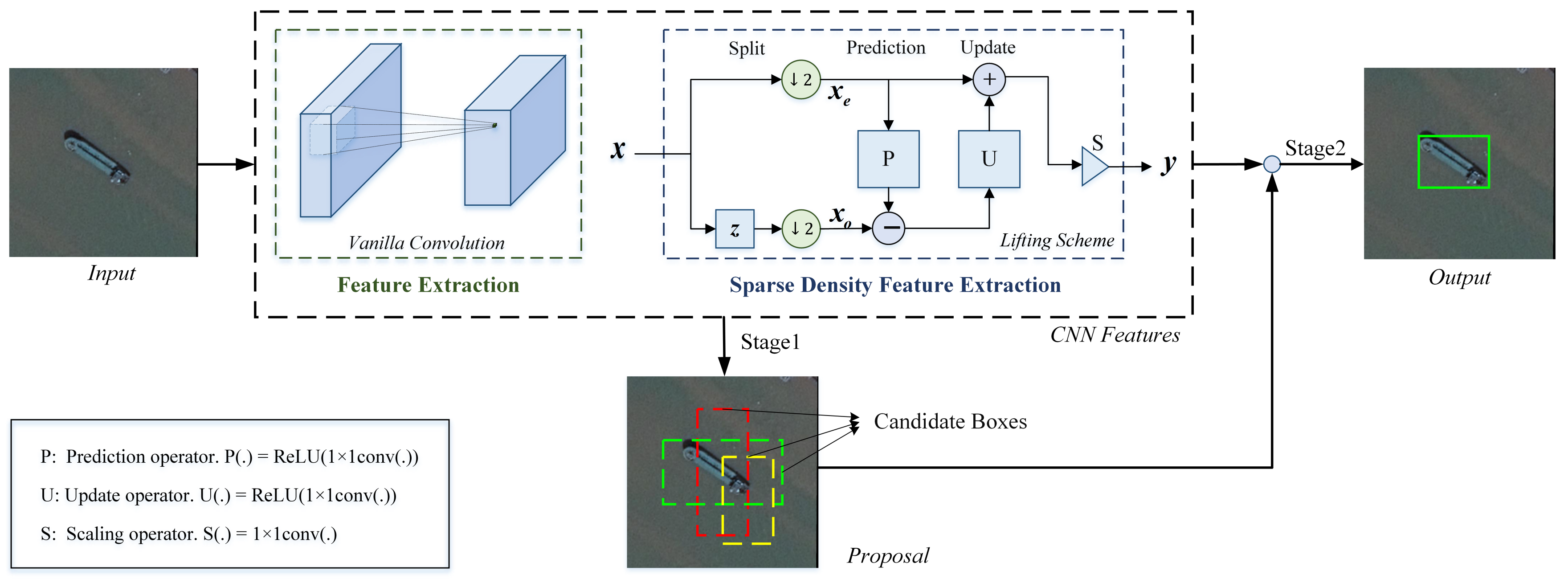
As shown in Figure 2b, both of the effects of applying the update operator and the scaling operator on a signal are multiplying this signal by a coefficient. These coefficients should be learnable and updated by the backpropagation algorithm to optimize the network representation ability. For simplicity and parallelization, we adopt the convolutional layer as U and S. The prediction operator P left shift the processed signal by one bit, which enhances the information contact between adjacent elements. To maintain the information contact property, an alternative for P is the convolutional layer. However, the convolutional layer is adopted as P in this paper to reduce the number of parameters and calculations.
The lifting scheme is a flexible algorithm to construct nonlinear wavelets. With the lifting scheme, the nonlinearity of pooling layer can be easily maintained by using nonlinear prediction and update operators. In this paper, ReLU function is used in P and U as nonlinear function. Therefore, the operators of the lifting scheme layer are as follows:
The 2D lifting scheme is implemented in a separable way, where the 1D lifting scheme is firstly applied on the rows and then on the columns of the 2D feature maps.
3.3. Lifting Scheme-Based Detection Network Flowchart
The proposed lifting scheme layer is a plug-and-play module that can be used as the feature extraction density reduction approach in both one stage and two stages detection network backbones without altering other modules. Figure 3 is the two stages detection network flowchart based on the lifting scheme layer. The backbone extracts features by vanilla Convolutional layers or the modules that are stacked by vanilla Convolutional layers, such as the basicBlock and the bottleNeck, in ResNet [3]. The lifting scheme layer is used in the modules that need to reduce feature extraction density, which can be an effective substitution for the commonly used strided convolutional layer or the vanilla convolutional layer followed by a pooling layer. CNN features are extracted by the backbone with these two kinds of modules, which are used in both of the two stages. In the first stage, some proposals are derived based on the CNN features and a selective algorithm. Then the category and the precise location of the objects are predicted with the CNN features and the proposals in the second stage.
4. Experimental Results
In military and civilian remote sensing target detection, aircraft and ship detection are usually of great practical value, among which ship detection has more datasets to evaluate the generalization ability and application prospect of the proposed method. Therefore, in this section, experiments are conducted on the remote sensing ship detection task on both the SAR image dataset and the optical remote sensing image dataset to evaluate the proposed lifting scheme-based sparse density feature extraction method.
4.1. Dataset Description
4.1.1. SAR Image Dataset
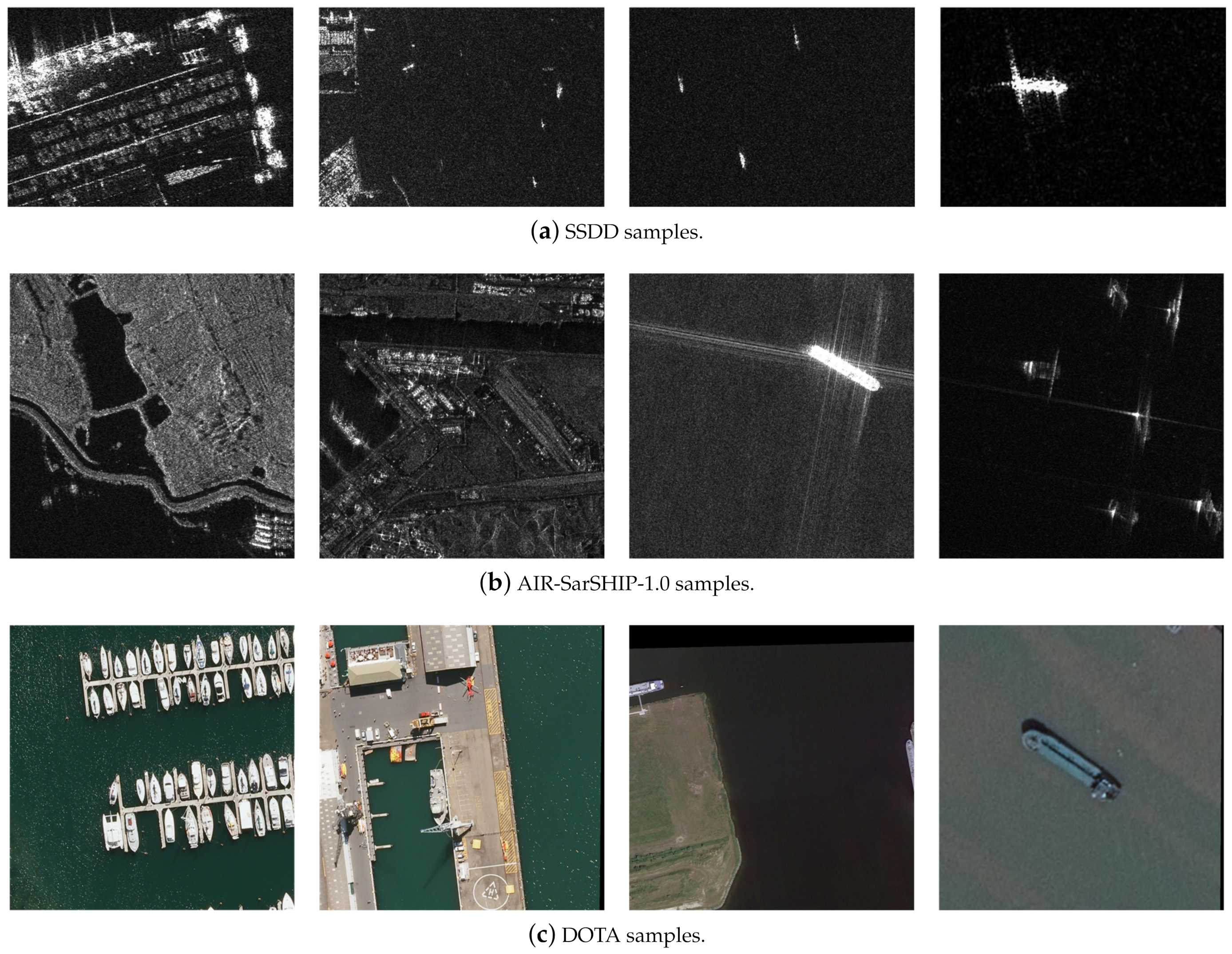
SSDD is a dataset of ships in SAR images, which contains a total of 1160 images and 2456 ships, and the average number of ships is 2.12. In SSDD, ships are in various environments, such as image resolution, ship size, sea condition, and sensor type, as shown in Figure 4a. The dataset is divided into a training set with 80% images from the total and a validation set with the rest images.
AIR-SarSHIP-1.0 is a wide-width SAR ship target public sample data set based on Gaofen-3 satellite data. The dataset contains 31 SAR images, and the scene types include ports, islands, reefs, and sea surfaces of different levels of sea conditions. Each image is cut into 36 slices, and each slice is resized to . The dataset contains 180 slices, where 70% are in the training set, while the rest slices are in the validation set. Samples from AIR-SarSHIP-1.0 dataset are shown in Figure 4b.
4.1.2. Optical Remote Sensing Image Dataset
The ship images in DOTA [26] are used as the single-class dataset for the optical remote sensing target detection experiment. DOTA is a large-scale dataset for object detection in aerial images, the size of each image of which ranges from to . In this paper, the images are divided into 1028 slices in the size of . The training set contains images from the total, while the validation set contains the rest images. Samples from the DOTA-ship dataset are shown in Figure 4c.
4.2. Evaluation Metrics
4.2.1. Detection Performance Metrics
Two universally agreed and standard metrics are used to evaluate the detection performance of the remote sensing target detection methods, namely precision-recall curve (PR curve) and average precision. These metrics are based on the overlapping area ratio (intersection over union, IOU) between detections and ground truth which is formulated as
Precision-recall curve (PR curve). The precision measures the percentage of true positives in the detected positive samples. The recall measures the percentage of the correctly detected positive samples in the ground truth. They are formulated as
where , , and denote true positive, false positive, and false negative, respectively.
In the object-level detection, a detection is labeled as true positive if IOU exceeds a predefined threshold . Otherwise, the detection is labeled as false positive. In this paper, is defined as .
Average precision (AP). The AP is the area under the PR curve that computes the average value of precision over the interval from recall = 0 to recall = 1. The higher AP value indicates the better detection performance. AP denotes the AP at .
4.2.2. Network Efficiency Metrics
It is important to evaluate the detection network efficiency for landing practical applications. In this paper, we use inference time to evaluate the detection speed, the number of parameters (#params) to evaluate the space occupancy, and billion float operations (BFLOPs) to measure the computational complexity.
4.3. Compared Methods
Baseline is Cascade R-CNN [34], whose backbone is ResNet-50 [3]. Another compared algorithm is Faster R-CNN [14]. Experimental results on SSDD and AIR-SarSHIP-1.0 are listed in Table 1 and Table 2, respectively.
In the experiments with baseline cascade R-CNN, we compare our proposed method Cascade R-CNN-LS with three sparse density feature extraction methods. The detailed illustrations are as follows.
- Cascade R-CNN. The baseline in the experiment. It is a two-stage detection network with the ResNet-50 backbone. Strided convolutional layer is the sparse density feature extraction module in the backbone.
- Cascade R-CNN-CP. The structure and settings are the same as the baseline except that the strided convolutional layer is substituted by a stride 1 convolutional layer (vanilla convolutional layer) followed by a pooling layer. Thus, this method is to evaluate the feature downsampling after extraction method and compare it with the strided convolution method. The pooling layer used in this paper is max-pooling.
- Cascade R-CNN-DCN. Deformable convolutional layer substitutes all of the stride 1 and strided convolutional layers with the size of in one module if its condition is set “True”. This network is to evaluate the effectiveness of the deformable convolution in remote sensing target detection and illustrate the advancement of our proposed method.
- Cascade R-CNN-LS. The proposed lifting scheme layer is used as the sparse density feature extraction module to replace the strided convolutional layer in the baseline. Other structures and settings of Cascade R-CNN-LS are the same as the baseline.
4.4. Results on SAR Image Datasets
The experimental results on the SAR image dataset SSDD and AIR-SarSHIP-1.0 are listed in Table 1 and Table 2, respectively. For both datasets, Cascade R-CNN-CP is superior to the baseline Cascade R-CNN with respect to the detection performance metric AP. However, the value of BFLOPs of Cascade R-CNN-CP is higher than Cascade R-CNN, which indicates higher computational complexity. These results draw the same conclusions as Springenberg et al. [15].
As Table 1 shows, our proposed lifting scheme method improves AP by compared with the baseline Cascade R-CNN while reducing BFLOPs compared with Cascade R-CNN-CP, verifying that our method achieves a better balance between detection precision and network efficiency. The proposed Cascade R-CNN-LS does not achieve an essential decrease in #Params and BFLOPs because there are only 5 layers in ResNet-50 that are altered by the lifting scheme layer for sparse density feature extraction. However, our method has the potential in improving the efficiency of backbones with more sparse density feature extraction layers. The deformable convolution-based method reaches an improvement over the baseline, but its number of parameters is larger, and it has lower AP compared with Cascade R-CNN-LS. The backbone of Faster R-CNN is ResNet-50 with stride 2 convolutional layer as the feature extraction density reduction module. As a plug-and-play module, the lifting scheme layer is also validated on another baseline, Faster R-CNN, to demonstrate its robustness with respect to different detection frameworks. The results show that Faster R-CNN-LS enhances the AP by with similar #Params and BFLOPs of the baseline.
The advancement of the proposed lifting scheme-based method is also verified on the AIR-SarSHIP-1.0 dataset as in Table 2. Cascade R-CNN-LS increases AP by over the baseline with fewer #Params and BFLOPs. It is noted that lifting scheme-based method (Cascade R-CNN-LS) even performs much better than the downsampling after extraction approach (Cascade R-CNN-CP). An explanation is that the lifting scheme is a similar implementation to the downsampling after extraction approach as proved in Section 3, but the lifting scheme layer is an adaptive layer whose parameters are updated during training, and the downsampling method in the lifting scheme layer is separable downsampling, instead of the max-pooling used in Cascade R-CNN-CP. We attribute the enhancement to these differences between these two methods.
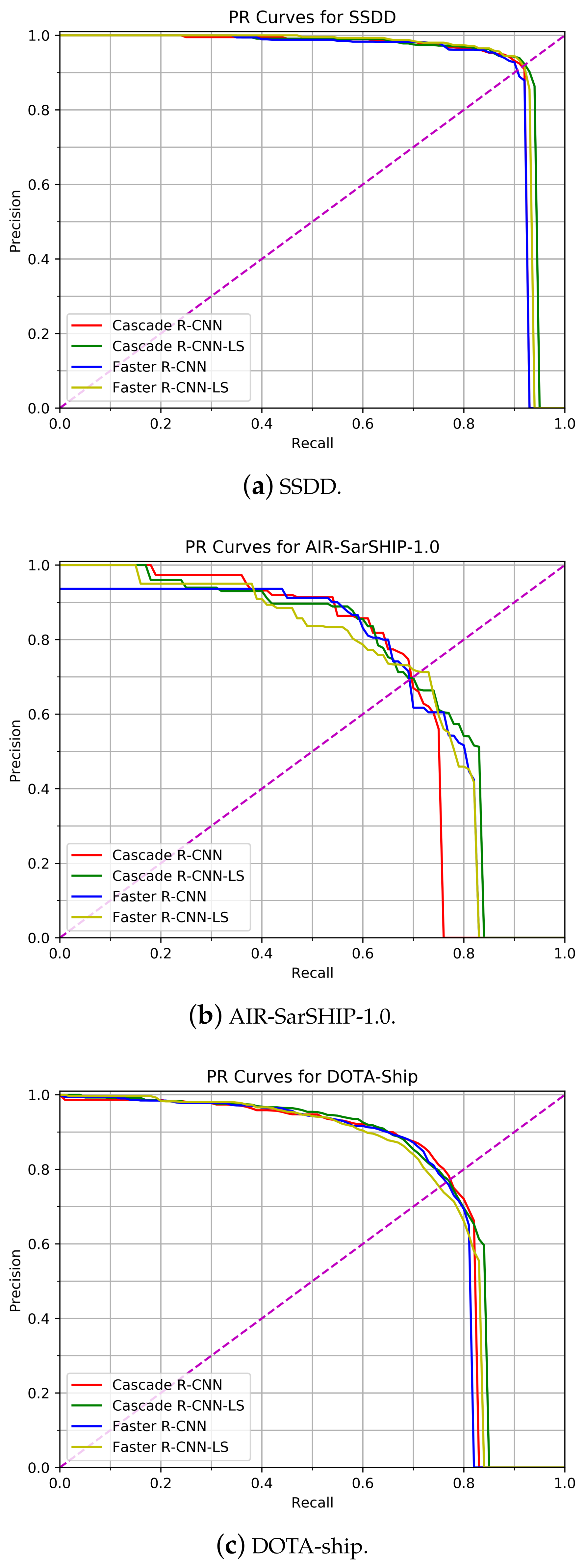
The superiority of Cascade R-CNN-LS in detection performance is also indicated by the RP curves in Figure 5a,b, where the lines of Cascade R-CNN-LS of both datasets are located at the top-right direction of the lines of baseline. For both datasets, the lifting scheme-based method reaches the best performance. For the same recall, networks with lifting scheme-based sparse density feature extraction method have higher precision, showing that our method is more sensitive to the slight differences between two similar objects and, thus, has less false alarm rate. On the other hand, the lifting scheme-based method has higher recall over baselines with the same precision, indicating that our method can detect more true targets. For Figure 5b, the deviations of different curves are larger than for other subfigures and the values of recall are particularly small. The reason is that target detection on AIR-SarSHIP-1.0 is more difficult than the other two datasets. The images in AIR-SARSHIP-1.0 have a high false alarm rate due to the land background interference. Because of the imaging principle of Gaofen-3, the dataset has a large intra-class variation on ship targets which leads to the small values of recall. Cascade R-CNN cannot handle these problems well and, thus, deviates greatly from other methods.
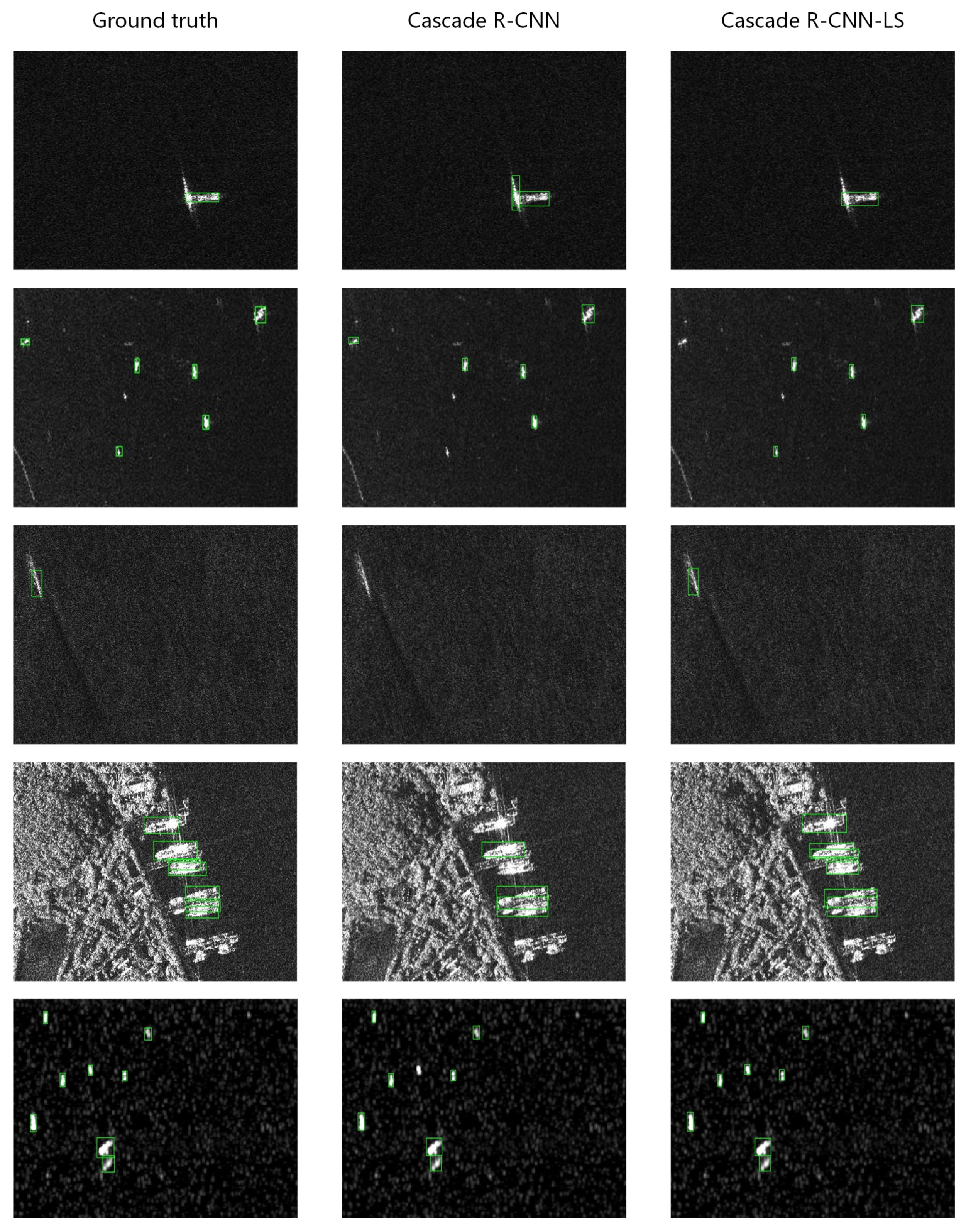
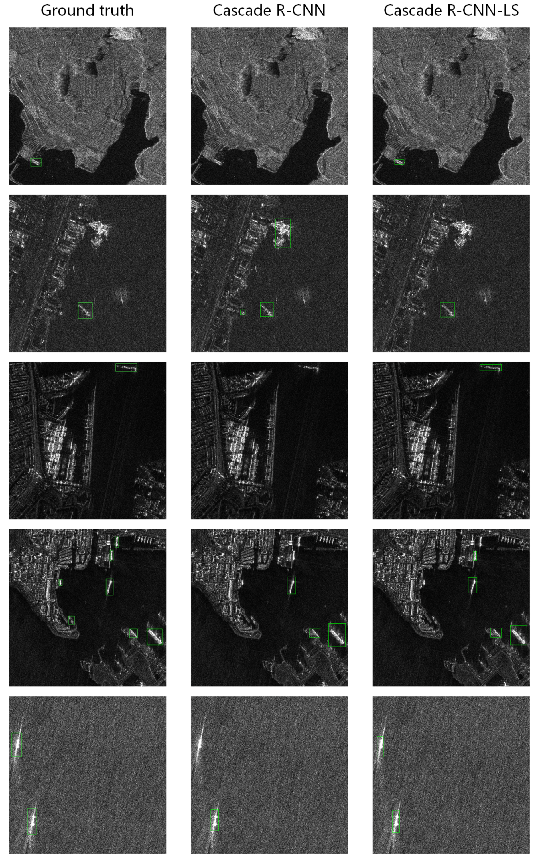
Figure 6 and Figure 7 show some detection results in the validation set of SSDD and AIR-SarSHIP-1.0, respectively. The ground truth, detection results of Cascade R-CNN and Cascade R-CNN-LS are displayed in the 1st, 2nd, and 3rd columns in these figures. For SSDD dataset, Cascade R-CNN fails to detect some targets as shown in the 2nd, 3rd, 4th, and 5th samples, while Cascade R-CNN-LS performs better both in small and middle size target detection. In addition, there is a false detection by Cascade R-CNN in the 1st sample. Cascade R-CNN-LS is also superior to Cascade R-CNN on AIR-SarSHIP-1.0 dataset as illustrated in Figure 7. In the 1st and 3rd samples, Cascade R-CNN fails to detect the targets, which are correctly detected by Cascade R-CNN-LS. In the 4th and 5th samples that contain multiple targets, Cascade R-CNN-LS correctly detects more targets than Cascade R-CNN. In the 2nd sample, false detection occurs with Cascade R-CNN, while it does not occur with Cascade R-CNN-LS. From these samples, it is observed that Cascade R-CNN-LS is more sensitive to small objects and able to detect these targets correctly. This is because Cascade R-CNN uses a strided convolutional layer to reduce feature density, which may lose the information about adjacent pixels and miss the small objects. In contrast, the lifting scheme has the advantage in the information contact between the adjacent pixels and, thus, tends to detect the small objects instead of missing them.
4.5. Results on Optical Remote Sensing Image Dataset
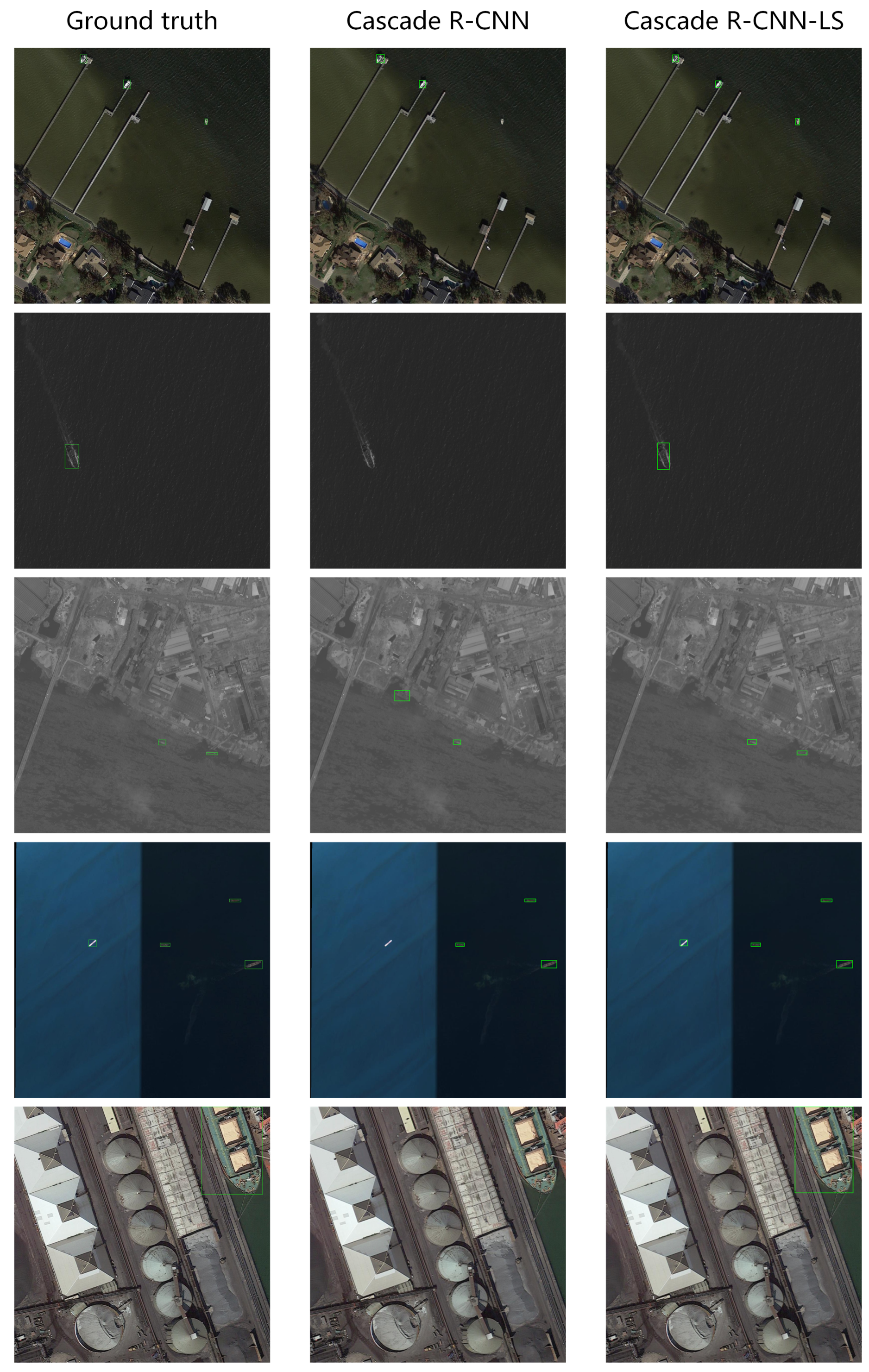
We conduct experiments on the DOTA-ship dataset to evaluate the applicability of the proposed method on the optical remote sensing target detection to verify that our approach is flexible to more application scenarios. Experimental results in Figure 5c and Table 3 show that the proposed method is superior to the strided convolution in both Cascade R-CNN and Faster R-CNN. Cascade R-CNN-LS and Faster R-CNN-LS have increased the AP by and , respectively, while they are more efficient than the relative baselines with respect to the metrices of inference time, number of parameters, and BFLOPs. Detection results of samples are shown in Figure 8, which indicates the proposed method reaches a better detection performance than the baseline. In the 1st and 4th samples in Figure 8, Cascade R-CNN fails to catch some small targets, while Cascade R-CNN-LS catches them correctly. In the 3rd sample, Cascade R-CNN misses a small target and has a false alarm, while the detection results of Cascade R-CNN-LS are the same as the ground truth. Cascade R-CNN even fails to detect some middle and big size targets as in the 2rd and 5th samples, which is inferior to Cascade R-CNN-LS.
5. Conclusions
This paper has introduced the lifting scheme into deep learning for remote sensing target detection and proposed a lifting scheme-based sparse density feature extraction method to achieve higher detection precision than the frequently used strided convolutional layer. This paper firstly proves that the lifting scheme has an inner relationship with the method that extracts features by a vanilla convolutional layer and then downsamples them by a pooling layer, and then a lifting scheme layer is constructed as the sparse density feature extraction method in the network backbone. Experimental results on both SAR and optical remote sensing image target detection indicate that the proposed method performs better than the strided convolutional layer in both computational complexity and detection precision. The lifting scheme-based sparse density feature extraction method is promising for remote sensing target detection.
Author Contributions
Conceptualization and funding acquisition, L.T.; Methodology, L.T. and Z.S.; Writing-original draft, Y.C., Z.S., and L.T.; Soft, B.H.; Project administration, C.H. and D.L.; Writing-review and editing, Z.S. and Y.C. All authors have read and agreed to the published version of the manuscript.
Funding
This research was funded by the National Natural Science Foundation of China (No. 41371342 and No. 61331016).
Institutional Review Board Statement
Not applicable.
Informed Consent Statement
Not applicable.
Data Availability Statement
No new data were created or analyzed in this study. Data sharing is not applicable to this article.
Conflicts of Interest
The authors declare no conflict of interest.
References
- Cheng, G.; Han, J. A survey on object detection in optical remote sensing images. ISPRS J. Photogramm. Remote Sens. 2016, 117, 11–28. [Google Scholar] [CrossRef] [Green Version]
- Simonyan, K.; Zisserman, A. Very deep convolutional networks for large-scale image recognition. arXiv 2014, arXiv:1409.1556. [Google Scholar]
- He, K.; Zhang, X.; Ren, S.; Sun, J. Deep residual learning for image recognition. In Proceedings of the IEEE Conference on Computer Vision and Pattern Recognition, Las Vegas, NV, USA, 27–30 June 2016; pp. 770–778. [Google Scholar]
- Iandola, F.; Moskewicz, M.; Karayev, S.; Girshick, R.; Darrell, T.; Keutzer, K. Densenet: Implementing efficient convnet descriptor pyramids. arXiv 2014, arXiv:1404.1869. [Google Scholar]
- Howard, A.G.; Zhu, M.; Chen, B.; Kalenichenko, D.; Wang, W.; Weyand, T.; Andreetto, M.; Adam, H. Mobilenets: Efficient convolutional neural networks for mobile vision applications. arXiv 2017, arXiv:1704.04861. [Google Scholar]
- Zhang, X.; Zhou, X.; Lin, M.; Sun, J. Shufflenet: An extremely efficient convolutional neural network for mobile devices. In Proceedings of the IEEE Conference on Computer Vision and Pattern Recognition, Salt Lake City, UT, USA, 18–23 June 2018; pp. 6848–6856. [Google Scholar]
- Iandola, F.N.; Han, S.; Moskewicz, M.W.; Ashraf, K.; Dally, W.J.; Keutzer, K. SqueezeNet: AlexNet-level accuracy with 50x fewer parameters and <0.5 MB model size. arXiv 2016, arXiv:1602.07360. [Google Scholar]
- LeCun, Y.; Bottou, L.; Bengio, Y.; Haffner, P. Gradient-based learning applied to document recognition. Proc. IEEE 1998, 86, 2278–2324. [Google Scholar] [CrossRef] [Green Version]
- Yu, F.; Koltun, V. Multi-scale context aggregation by dilated convolutions. arXiv 2015, arXiv:1511.07122. [Google Scholar]
- Dai, J.; Qi, H.; Xiong, Y.; Li, Y.; Zhang, G.; Hu, H.; Wei, Y. Deformable convolutional networks. In Proceedings of the IEEE International Conference on Computer Vision, Venice, Italy, 22–29 October 2017; pp. 764–773. [Google Scholar]
- Redmon, J.; Divvala, S.; Girshick, R.; Farhadi, A. You only look once: Unified, real-time object detection. In Proceedings of the IEEE Conference on Computer Vision and Pattern Recognition, Las Vegas, NV, USA, 27–30 June 2016; pp. 779–788. [Google Scholar]
- Redmon, J.; Farhadi, A. YOLO9000: Better, faster, stronger. In Proceedings of the IEEE International Conference on Computer Vision, Venice, Italy, 22–29 October 2017; pp. 7263–7271. [Google Scholar]
- Redmon, J.; Farhadi, A. Yolov3: An incremental improvement. arXiv 2018, arXiv:1804.02767. [Google Scholar]
- Ren, S.; He, K.; Girshick, R.; Sun, J. Faster r-cnn: Towards real-time object detection with region proposal networks. In Proceedings of the NIPS’15: Proceedings of the 28th International Conference on Neural Information Processing Systems, Bali, Indonesia, 8–12 December 2021; pp. 91–99. [Google Scholar]
- Springenberg, J.T.; Dosovitskiy, A.; Brox, T.; Riedmiller, M. Striving for simplicity: The all convolutional net. arXiv 2014, arXiv:1412.6806. [Google Scholar]
- Sweldens, W. Lifting scheme: A new philosophy in biorthogonal wavelet constructions. In Proceedings of the International Society for Optics and Photonics, San Diego, CA, USA, 9–14 July 1995; Volume 2569, pp. 68–80. [Google Scholar]
- Sweldens, W. The lifting scheme: A custom-design construction of biorthogonal wavelets. Appl. Comput. Harmon. Anal. 1996, 3, 186–200. [Google Scholar] [CrossRef] [Green Version]
- Sweldens, W. The lifting scheme: A construction of second generation wavelets. SIAM J. Math. Anal. 1998, 29, 511–546. [Google Scholar] [CrossRef] [Green Version]
- Heijmans, H.J.; Goutsias, J. Nonlinear multiresolution signal decomposition schemes. II. Morphological wavelets. IEEE Trans. Image Process. 2000, 9, 1897–1913. [Google Scholar] [CrossRef] [PubMed] [Green Version]
- Zheng, Y.; Wang, R.; Li, J. Nonlinear wavelets and bp neural networks adaptive lifting scheme. In Proceedings of the 2010 International Conference on Apperceiving Computing and Intelligence Analysis Proceeding, Chengdu, China, 17–19 December 2010; pp. 316–319. [Google Scholar]
- Calderbank, A.; Daubechies, I.; Sweldens, W.; Yeo, B.L. Wavelet transforms that map integers to integers. Appl. Comput. Harmon. Anal. 1998, 5, 332–369. [Google Scholar] [CrossRef] [Green Version]
- Daubechies, I.; Sweldens, W. Factoring wavelet transforms into lifting steps. J. Fourier Anal. Appl. 1998, 4, 247–269. [Google Scholar] [CrossRef]
- He, C.; Shi, Z.; Qu, T.; Wang, D.; Liao, M. Lifting Scheme-Based Deep Neural Network for Remote Sensing Scene Classification. Remote Sens. 2019, 11, 2648. [Google Scholar] [CrossRef] [Green Version]
- Li, J.; Qu, C.; Shao, J. Ship detection in SAR images based on an improved faster R-CNN. In Proceedings of the 2017 SAR in Big Data Era: Models, Methods and Applications (BIGSARDATA), Beijing, China, 13–14 November 2017; pp. 1–6. [Google Scholar]
- Xian, S.; Zhirui, W.; Yuanrui, S.; Wenhui, D.; Yue, Z.; Kun, F. AIR-SARShip–1.0: High Resolution SAR Ship Detection Dataset. J. Radars 2019, 8, 852–862. [Google Scholar]
- Xia, G.S.; Bai, X.; Ding, J.; Zhu, Z.; Belongie, S.; Luo, J.; Datcu, M.; Pelillo, M.; Zhang, L. DOTA: A Large-Scale Dataset for Object Detection in Aerial Images. In Proceedings of the IEEE Conference on Computer Vision and Pattern Recognition (CVPR), Salt Lake City, UT, USA, 18–22 June 2018. [Google Scholar]
- Girshick, R.; Donahue, J.; Darrell, T.; Malik, J. Rich feature hierarchies for accurate object detection and semantic segmentation. In Proceedings of the IEEE Conference on Computer Vision and Pattern Recognition, Columbus, OH, USA, 23–28 June 2014; pp. 580–587. [Google Scholar]
- Girshick, R. Fast r-cnn. In Proceedings of the IEEE Conference on Computer Vision and Pattern Recognition, Boston, MA, USA, 7–12 June 2015; pp. 1440–1448. [Google Scholar]
- Liu, W.; Anguelov, D.; Erhan, D.; Szegedy, C.; Reed, S.; Fu, C.Y.; Berg, A.C. Ssd: Single shot multibox detector. In Proceedings of the European Conference on Computer Vision, Amsterdam, The Netherlands, 8–16 October 2016; pp. 21–37. [Google Scholar]
- Glorot, X.; Bordes, A.; Bengio, Y. Deep sparse rectifier neural networks. In Proceedings of the Fourteenth International Conference on Artificial Intelligence and Statistics, Ft. Lauderdale, FL, USA, 11–13 April 2011; pp. 315–323. [Google Scholar]
- Krizhevsky, A.; Sutskever, I.; Hinton, G.E. Imagenet classification with deep convolutional neural networks. In Proceedings of the 26th Annual Conference on Neural Information Processing Systems, Lake Tahoe, NV, USA, 3–6 December 2012; pp. 1097–1105. [Google Scholar]
- Mallat, S.G. A theory for multiresolution signal decomposition: The wavelet representation. IEEE Trans. Pattern Anal. Mach. Intell. 1989, 11, 674–693. [Google Scholar] [CrossRef] [Green Version]
- Oppenheim, A.V.; Schafer, R.W. Discrete—Time Signal Processing; Pearson: Chennai, India, 1977. [Google Scholar]
- Cai, Z.; Vasconcelos, N. Cascade r-cnn: Delving into high quality object detection. In Proceedings of the IEEE Conference on Computer Vision and Pattern Recognition, Salt Lake City, UT, USA, 18–22 June 2018; pp. 6154–6162. [Google Scholar]
Figure 1.
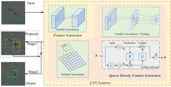
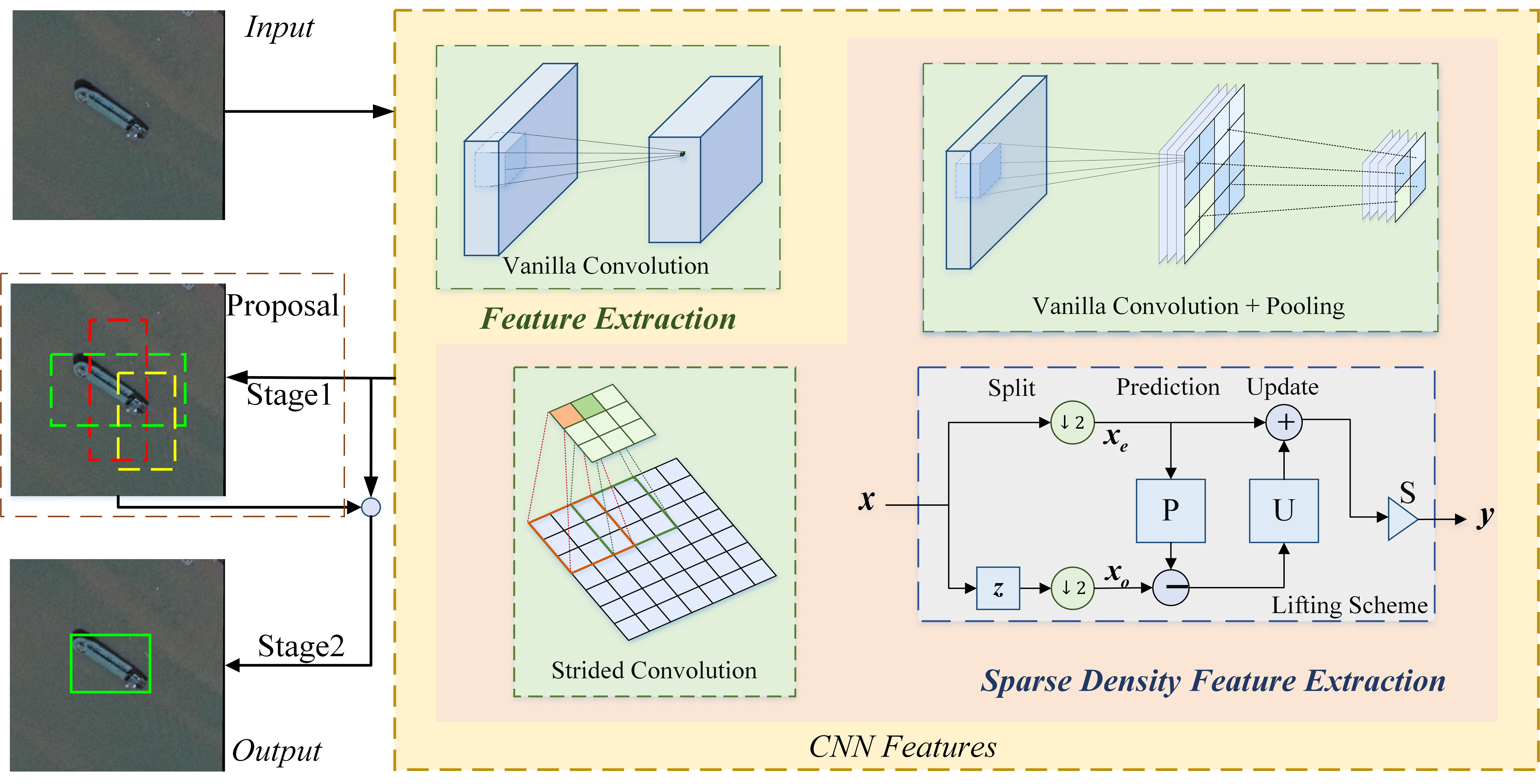
Typical remote sensing target detection flowchart. There are mainly two types of target detection networks, including two-stage (containing both Stage1 in the dashed box and Stage2) and one-stage networks (containing Stage2 only). For both of them, convolutional neural networks are the most common backbones for feature extraction. The vanilla convolution with the stride of one is repeatedly used in the backbone for normal density feature extraction. The sparse density feature extraction module is for receptive field enlargement and dimension reduction, concrete existing approaches of which are vanilla convolutional layer followed by a pooling layer (which is denoted as downsampling after extraction approach in this paper), dilated convolution, deformable convolution, and the most frequently used method—strided convolution, etc.
Figure 1.
Typical remote sensing target detection flowchart. There are mainly two types of target detection networks, including two-stage (containing both Stage1 in the dashed box and Stage2) and one-stage networks (containing Stage2 only). For both of them, convolutional neural networks are the most common backbones for feature extraction. The vanilla convolution with the stride of one is repeatedly used in the backbone for normal density feature extraction. The sparse density feature extraction module is for receptive field enlargement and dimension reduction, concrete existing approaches of which are vanilla convolutional layer followed by a pooling layer (which is denoted as downsampling after extraction approach in this paper), dilated convolution, deformable convolution, and the most frequently used method—strided convolution, etc.

Figure 2.
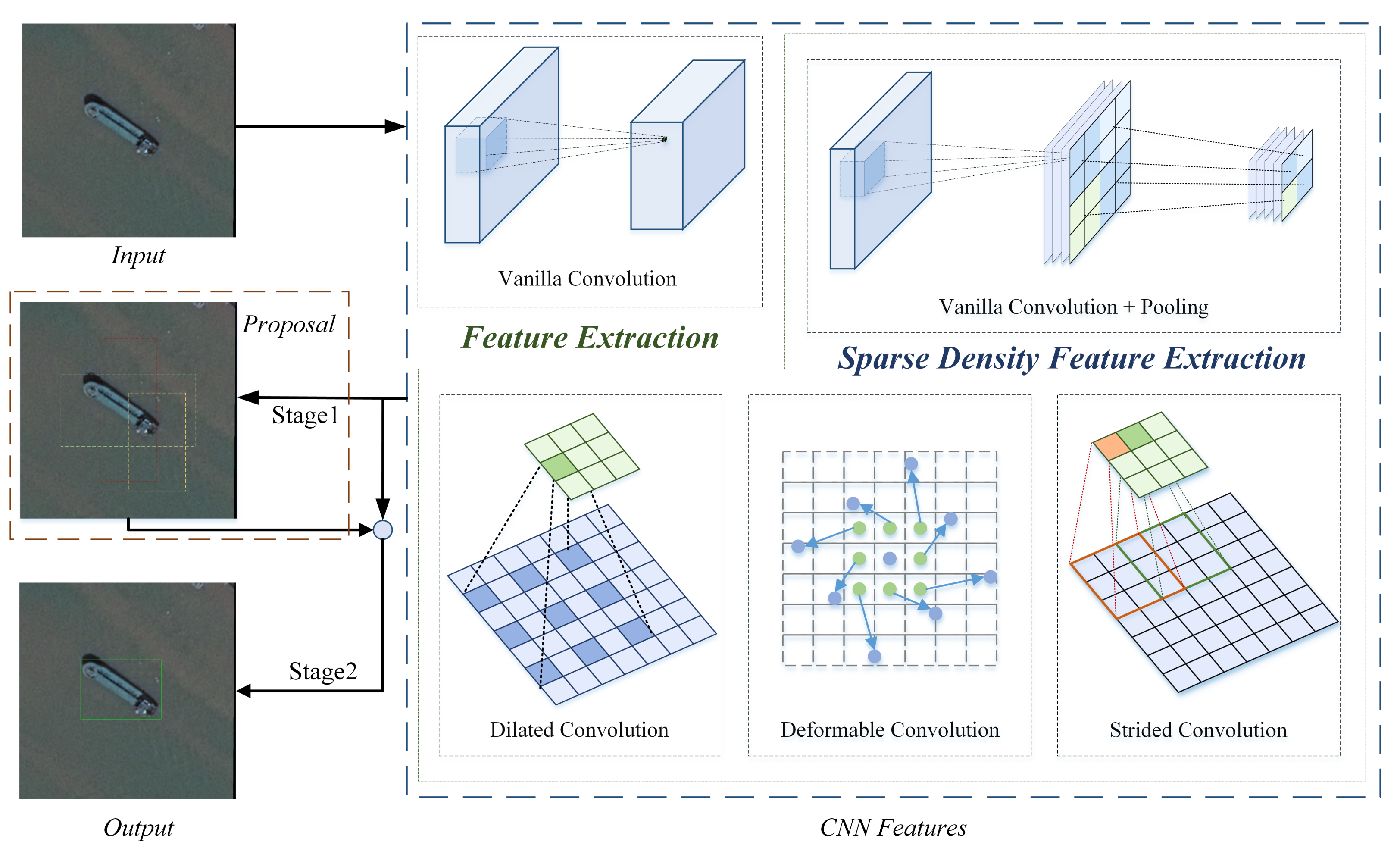
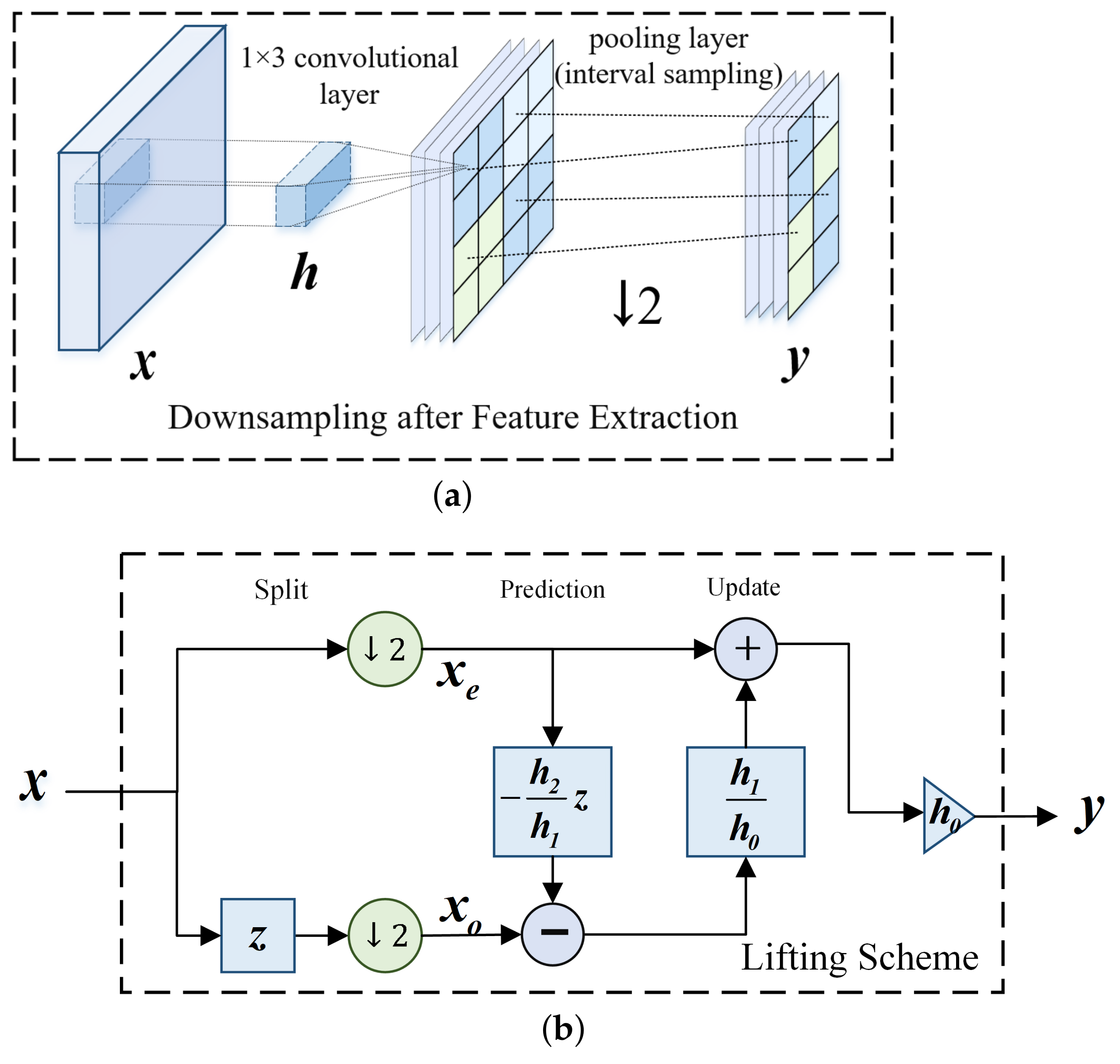
The method of downsampling after extraction is generally implemented with a vanilla convolutional layer and a pooling layer, while the lifting scheme is another alternative implementation. The symbols , , and denote the input signal, convolutional kernel, and output signal, respectively. The lifting scheme contains three steps: split, prediction and update. These two methods have the same and theoretically, and in (a) is transformed into the prediction and update operators as showned in (b).
Figure 2.
The method of downsampling after extraction is generally implemented with a vanilla convolutional layer and a pooling layer, while the lifting scheme is another alternative implementation. The symbols , , and denote the input signal, convolutional kernel, and output signal, respectively. The lifting scheme contains three steps: split, prediction and update. These two methods have the same and theoretically, and in (a) is transformed into the prediction and update operators as showned in (b).

Figure 3.
Two stage detection network flowchart based on lifting scheme layer. Different from the existing two-stage detection networks, the lifting scheme layer is used as the sparse density feature extraction module in the backbone CNN, which is superior to the frequently used strided convolution in detection precision. A series of candidate boxes are generated in the first stage, and then they are classified in the second stage. The candidate box that is classified as a ship and exceeds the IOU threshold is reserved in the output.

Figure 4.
Samples from the datasets. Three remote sensing ship datasets are used in the experiments to evaluate the proposed method, including two SAR datasets SSDD and AIR-SarSHIP-1.0, and one optical remote sensing image dataset DOTA-ship.
Figure 4.
Samples from the datasets. Three remote sensing ship datasets are used in the experiments to evaluate the proposed method, including two SAR datasets SSDD and AIR-SarSHIP-1.0, and one optical remote sensing image dataset DOTA-ship.

Figure 5.
Precision-recall curves on three remote sensing image datasets of two pairs of detection networks, including (1) Cascade R-CNN and Cascade R-CNN-LS, (2) Faster R-CNN and Faster R-CNN-LS. For all the datasets, Cascade R-CNN-LS consistently performs the best, and the lifting scheme-based method is superior to the strided convolution in both experiments with the baselines of Cascade R-CNN and Faster R-CNN.

Figure 6.
Detection results on SSDD samples. The 1st column displays the samples from the ground truth, while the 2nd and 3rd columns are the detection results of the relative samples of Cascade R-CNN and Cascade R-CNN-LS, respectively. The lifting scheme-based network tends to detect small objects better than the strided convolution as the 2nd and the 5th rows show.

Figure 7.
Detection results on AIR-SarSHIP-1.0 samples. The 1st column displays the samples from the ground truth, while the 2nd and 3rd columns are the detection results of the relative samples of Cascade R-CNN and Cascade R-CNN-LS, respectively. The lifting scheme-based network tends to detect small objects better than the strided convolution as the 1st and the 3rd rows show.

Figure 8.
Detection results on DOTA-ship samples. The 1st column displays the samples from the ground truth, while the 2nd and 3rd columns are the detection results of the relative samples of Cascade R-CNN and Cascade R-CNN-LS, respectively. The lifting scheme-based network detects targets correctly in these samples, while Cascade R-CNN fails to detect some small, middle, and large size targets and has false alarms.


Table 1.
Experiment results on SSDD with Cascade R-CNN and Faster R-CNN as baselines. The postfixes of “CP”, “DCN”, and “LS” in the Method column indicate the different sparse density feature extraction modules in the network, which are pooling after extraction, deformable convolution, and the proposed lifting scheme layer, respectively. The evaluation metrics include detection performance metrics of average precision at IOU threshold = 0.5 (AP) and network efficiency metrics of inference time (IT), the number of parameters (#params), and billion float operations (BFLOPs). The values in the parentheses in the AP column represent the increment compared with the baselines. The best results are in bold.
| Method | Backbone | AP (%) | IT (ms) | #Params (MB) | BFLOPs |
|---|---|---|---|---|---|
| Cascade R-CNN | ResNet-50 | 90.8 | 46.3 | 552 | 91.05 |
| Cascade R-CNN-CP | ResNet-50-CP | 92.8 (+2.0) | 38 | 552.6 | 96.49 |
| Cascade R-CNN-DCN | ResNet-50-DCN | 92.1 (+1.3) | 43 | 557 | 83.86 |
| Cascade R-CNN-LS | ResNet-50-LS | 92.6 (+1.8) | 39 | 541 | 90.65 |
| Faster R-CNN | ResNet-50 | 90.6 | 37.5 | 330 | 63.66 |
| Faster R-CNN-LS | ResNet-50-LS | 92.0 (+1.4) | 34.6 | 322.5 | 63.26 |
Table 2.
Experiment results on AIR-SarSHIP-1.0. The postfixes of “CP”, “DCN”, and “LS” in the Method column indicate the different sparse density feature extraction modules in the network, which are pooling after extraction, deformable convolution, and the proposed lifting scheme layer, respectively. The evaluation metrics include detection performance metrics of average precision at IOU threshold = 0.5 (AP) and network efficiency metrics of inference time (IT), the number of parameters (#params), and billion float operations (BFLOPs). The values in the parentheses in the AP column represent the increment compared with the baselines. The best results are in bold.
| Method | Backbone | AP (%) | IT (ms) | #Params (MB) | BFLOPs |
|---|---|---|---|---|---|
| Cascade R-CNN | ResNet-50 | 67.8 | 55.55 | 552 | 91.05 |
| Cascade R-CNN-CP | ResNet-50-CP | 68.3 (+0.5) | 54 | 552.6 | 96.49 |
| Cascade R-CNN-DCN | ResNet-50-DCN | 69.6 (+1.8) | 55 | 557 | 83.86 |
| Cascade R-CNN-LS | ResNet-50-LS | 72.0 (+4.2) | 37 | 541 | 90.65 |
| Faster R-CNN | ResNet-50 | 70.0 | 37 | 330 | 63.66 |
| Faster R-CNN-LS | ResNet-50-LS | 70.1 (+0.1) | 37.3 | 322.5 | 63.26 |
Table 3.
Experiment results on DOTA with Cascade R-CNN and Faster R-CNN as baselines. The postfixes of “CP” and “LS” in the Method column indicate the different sparse density feature extraction modules in the network, which are pooling after extraction and the proposed lifting scheme layer, respectively. The evaluation metrics include detection performance metrics of average precision at IOU threshold = 0.5 (AP) and network efficiency metrics of inference time (IT), the number of parameters (#params), and billion float operations (BFLOPs). The values in the parentheses in the AP column represent the increment compared with the baselines. The best results are in bold.
| Method | Backbone | AP (%) | IT (ms) | #Params (MB) | BFLOPs |
|---|---|---|---|---|---|
| Cascade R-CNN | ResNet-50 | 76.6 | 44.49 | 552 | 91.05 |
| Cascade R-CNN-CP | ResNet-50-CP | 77.8 (+1.2) | 40 | 552.6 | 96.49 |
| Cascade R-CNN-LS | ResNet-50-LS | 77.9 (+1.3) | 45 | 541 | 90.65 |
| Faster R-CNN | ResNet-50 | 75.8 | 44.8 | 330 | 63.66 |
| Faster R-CNN-LS | ResNet-50-LS | 76.5 (+0.7) | 40 | 322.5 | 63.26 |
Publisher’s Note: MDPI stays neutral with regard to jurisdictional claims in published maps and institutional affiliations. |
© 2021 by the authors. Licensee MDPI, Basel, Switzerland. This article is an open access article distributed under the terms and conditions of the Creative Commons Attribution (CC BY) license (https://creativecommons.org/licenses/by/4.0/).
Share and Cite
MDPI and ACS Style
Tian, L.; Cao, Y.; Shi, Z.; He, B.; He, C.; Li, D. Lifting Scheme-Based Sparse Density Feature Extraction for Remote Sensing Target Detection. Remote Sens. 2021, 13, 1862. https://0-doi-org.brum.beds.ac.uk/10.3390/rs13091862
AMA Style
Tian L, Cao Y, Shi Z, He B, He C, Li D. Lifting Scheme-Based Sparse Density Feature Extraction for Remote Sensing Target Detection. Remote Sensing. 2021; 13(9):1862. https://0-doi-org.brum.beds.ac.uk/10.3390/rs13091862
Chicago/Turabian StyleTian, Ling, Yu Cao, Zishan Shi, Bokun He, Chu He, and Deshi Li. 2021. "Lifting Scheme-Based Sparse Density Feature Extraction for Remote Sensing Target Detection" Remote Sensing 13, no. 9: 1862. https://0-doi-org.brum.beds.ac.uk/10.3390/rs13091862
Note that from the first issue of 2016, this journal uses article numbers instead of page numbers. See further details here.