
Can Forel–Ule Index Act as a Proxy of Water Quality in Temperate Waters? Application of Plume Mapping in Liverpool Bay, UK

 , , ,
, , ,  and
and
Abstract
:1. Introduction
2. Materials and Methods
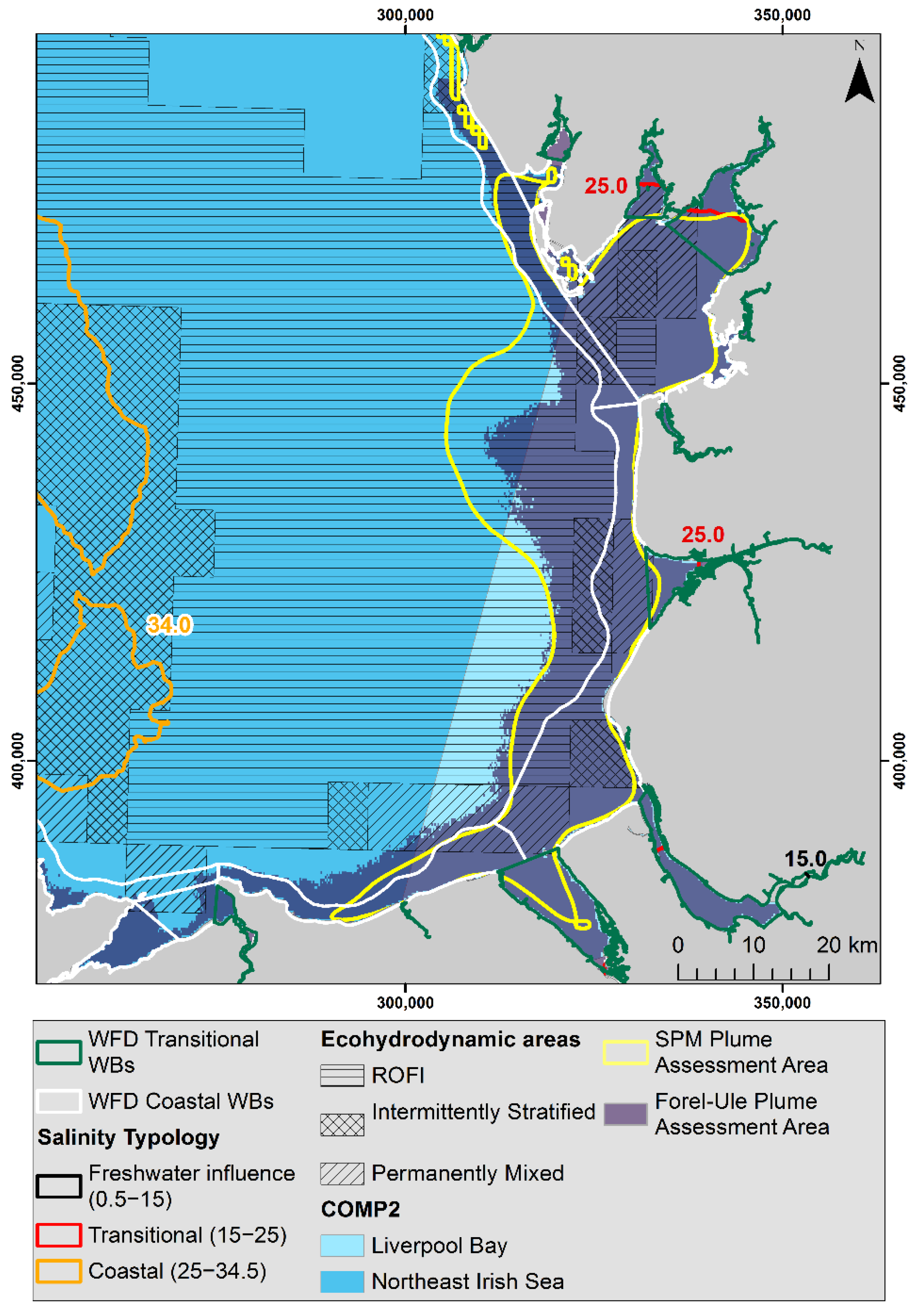
2.1. Study Area
2.2. Water Quality Monitoring
2.3. River Flow Data
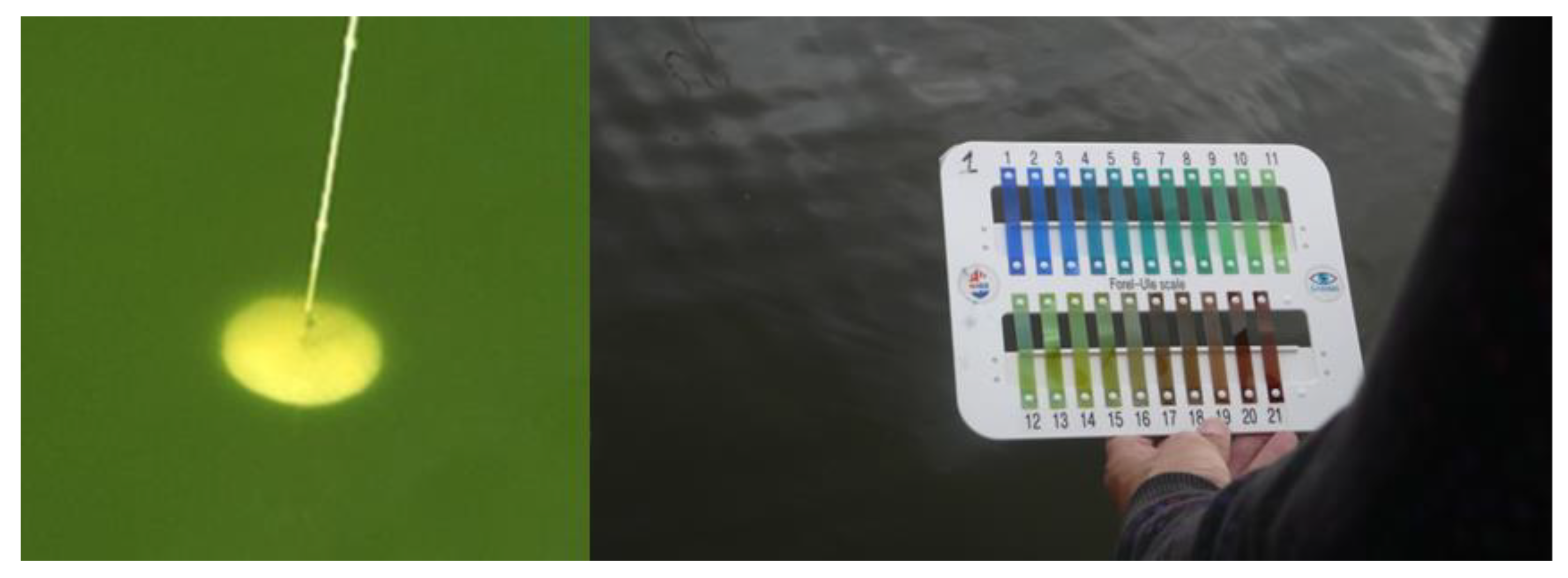
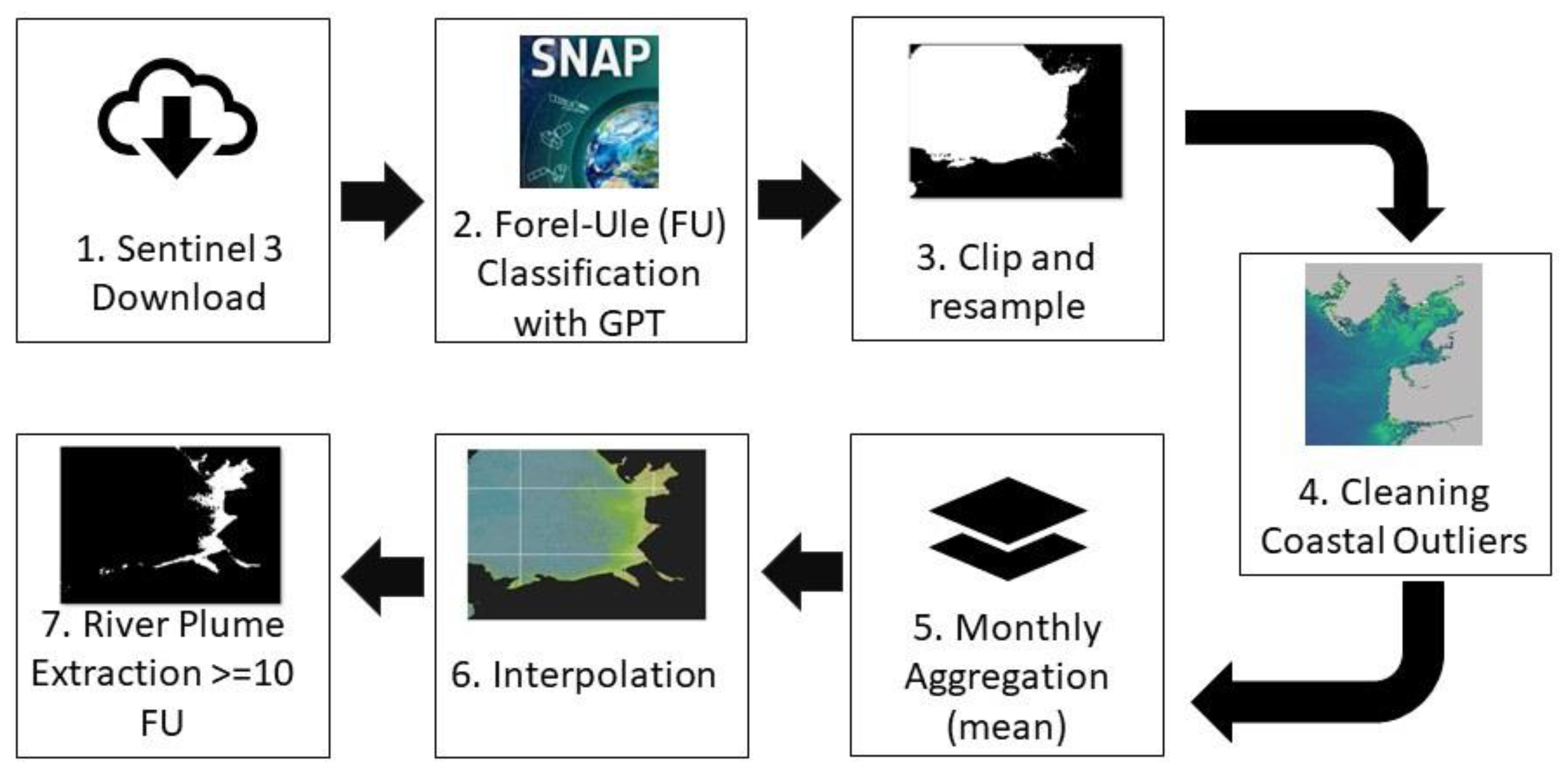
2.4. FUI Satellite Mapping of Water Type
2.5. FUI Batch Processing
3. Results
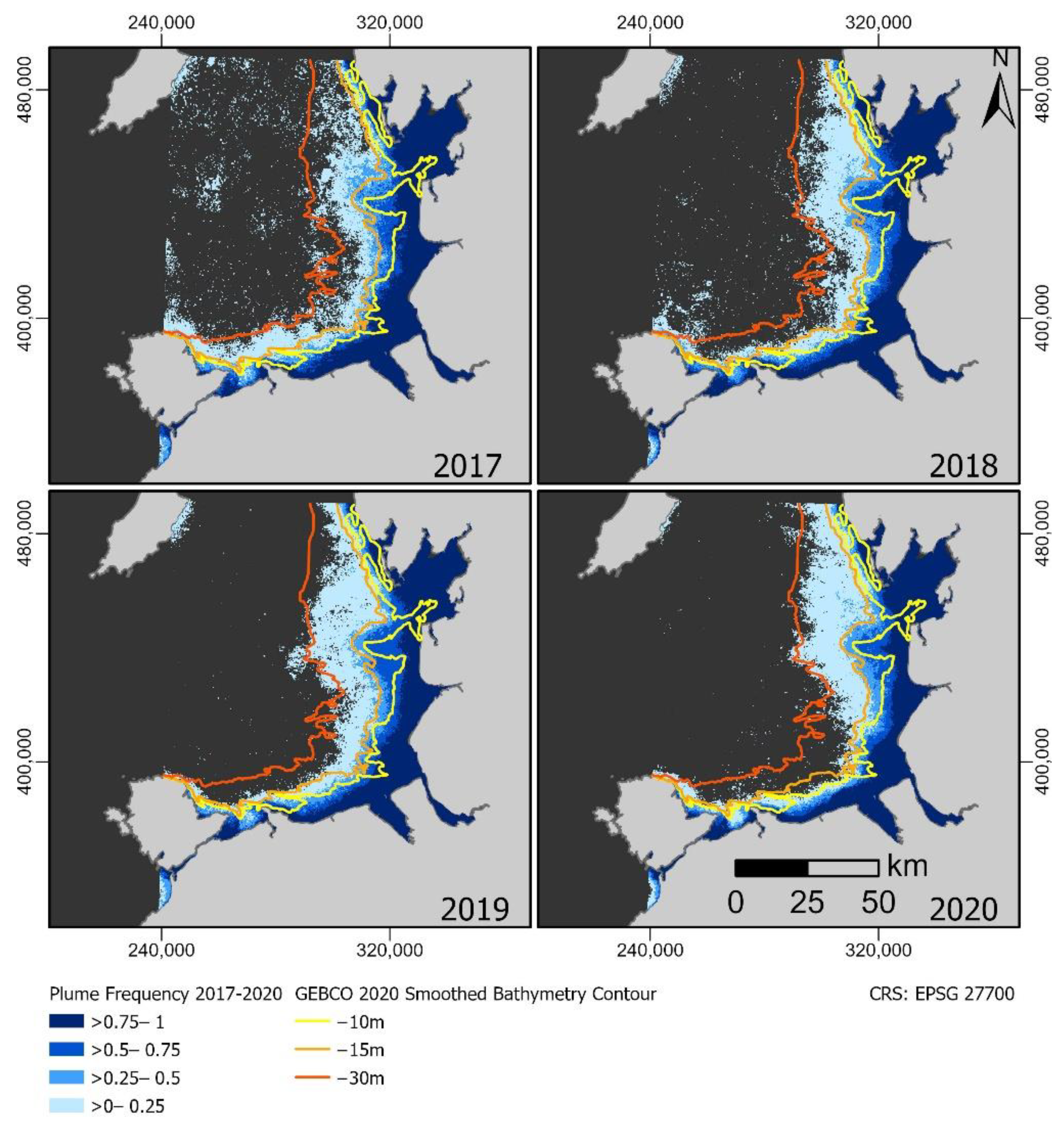
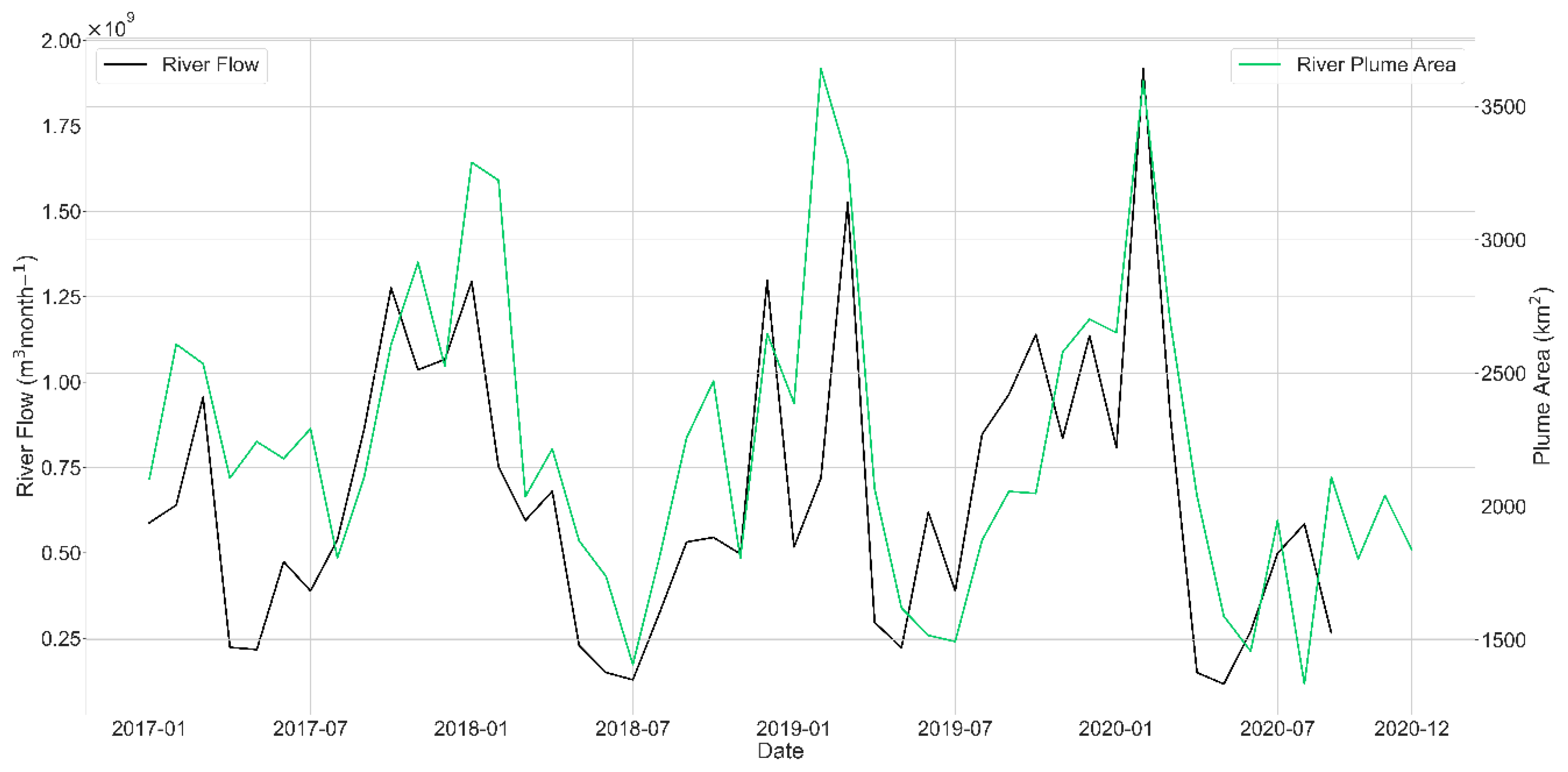
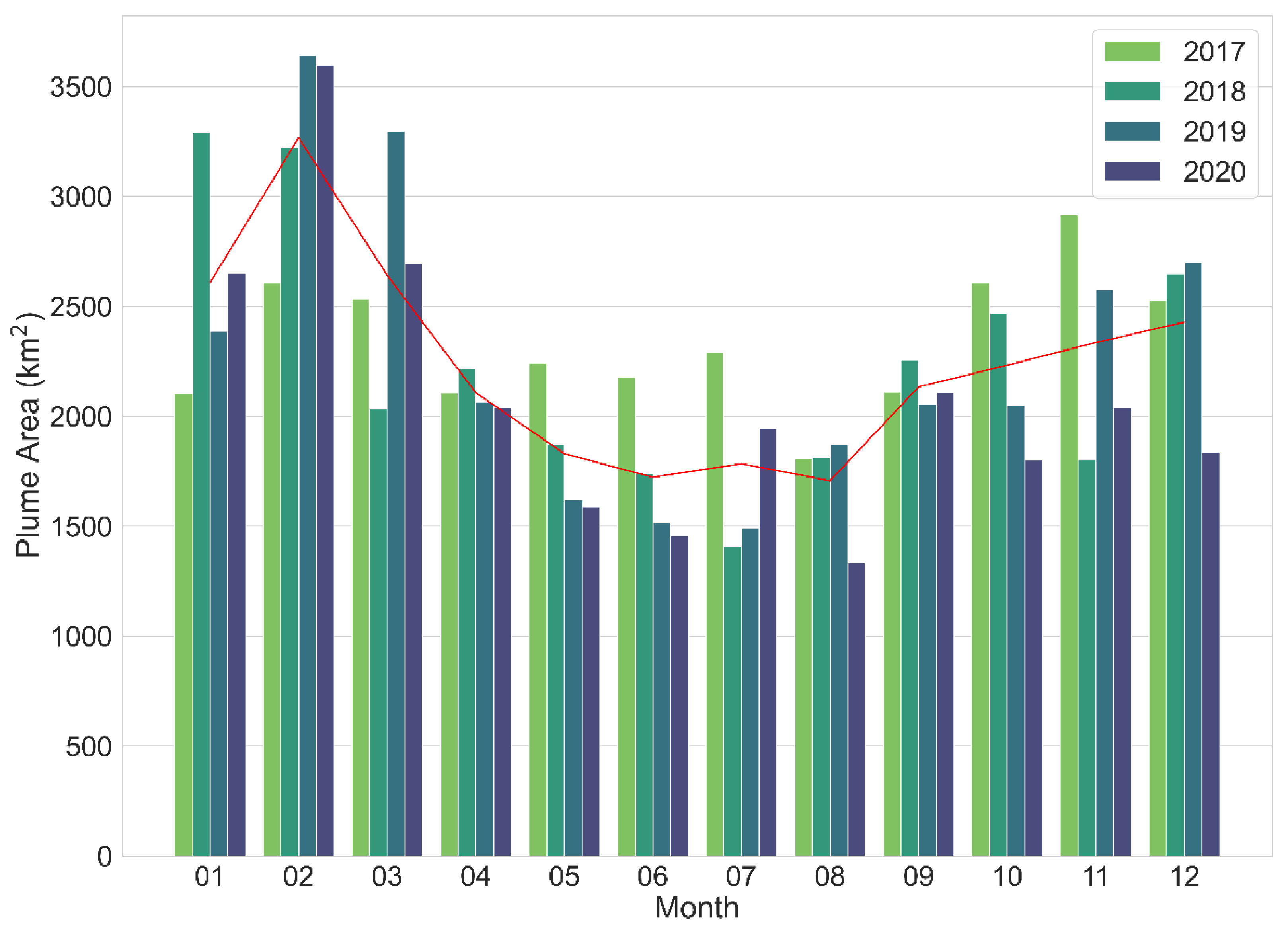
3.1. Plume Extent
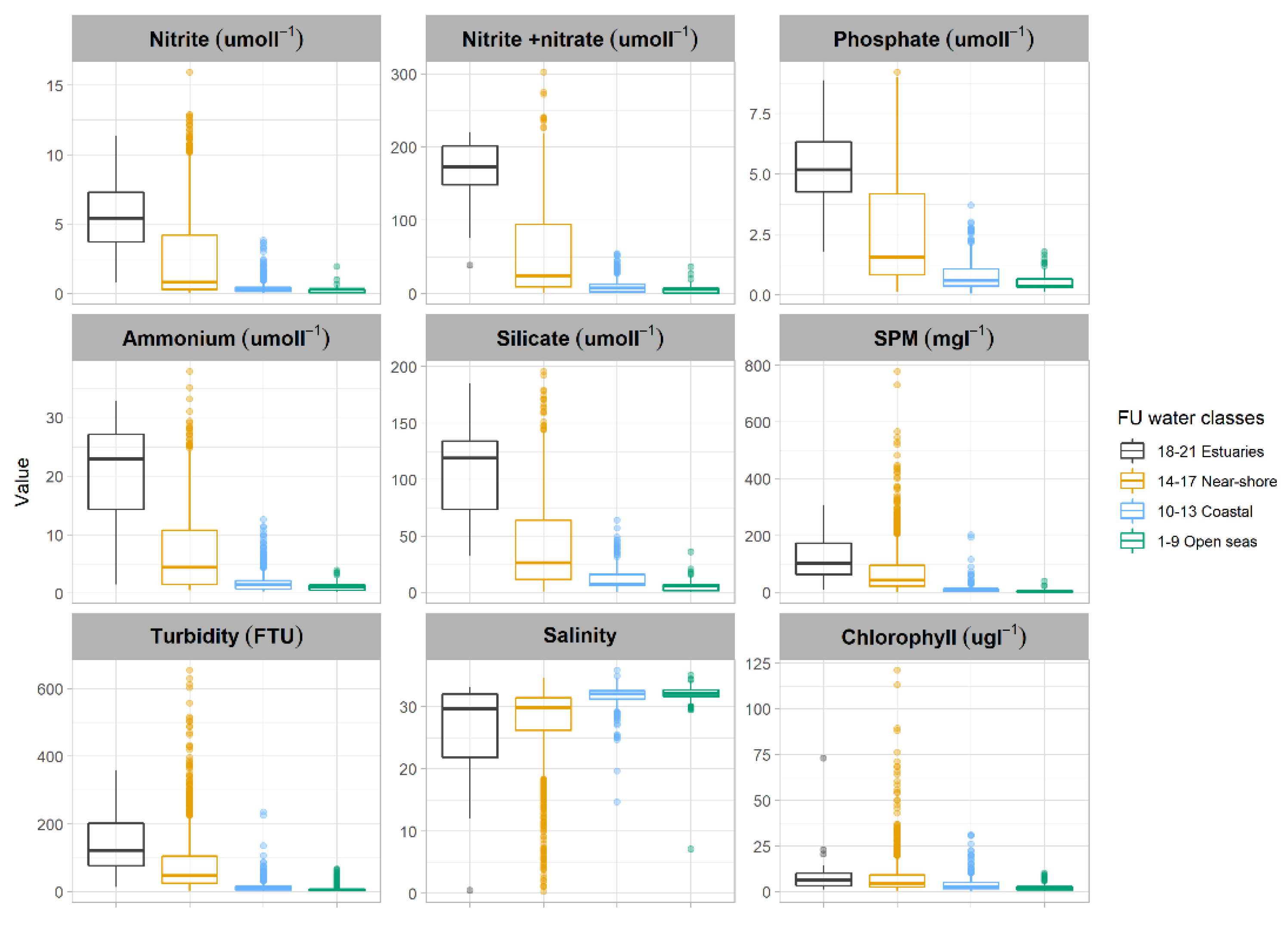
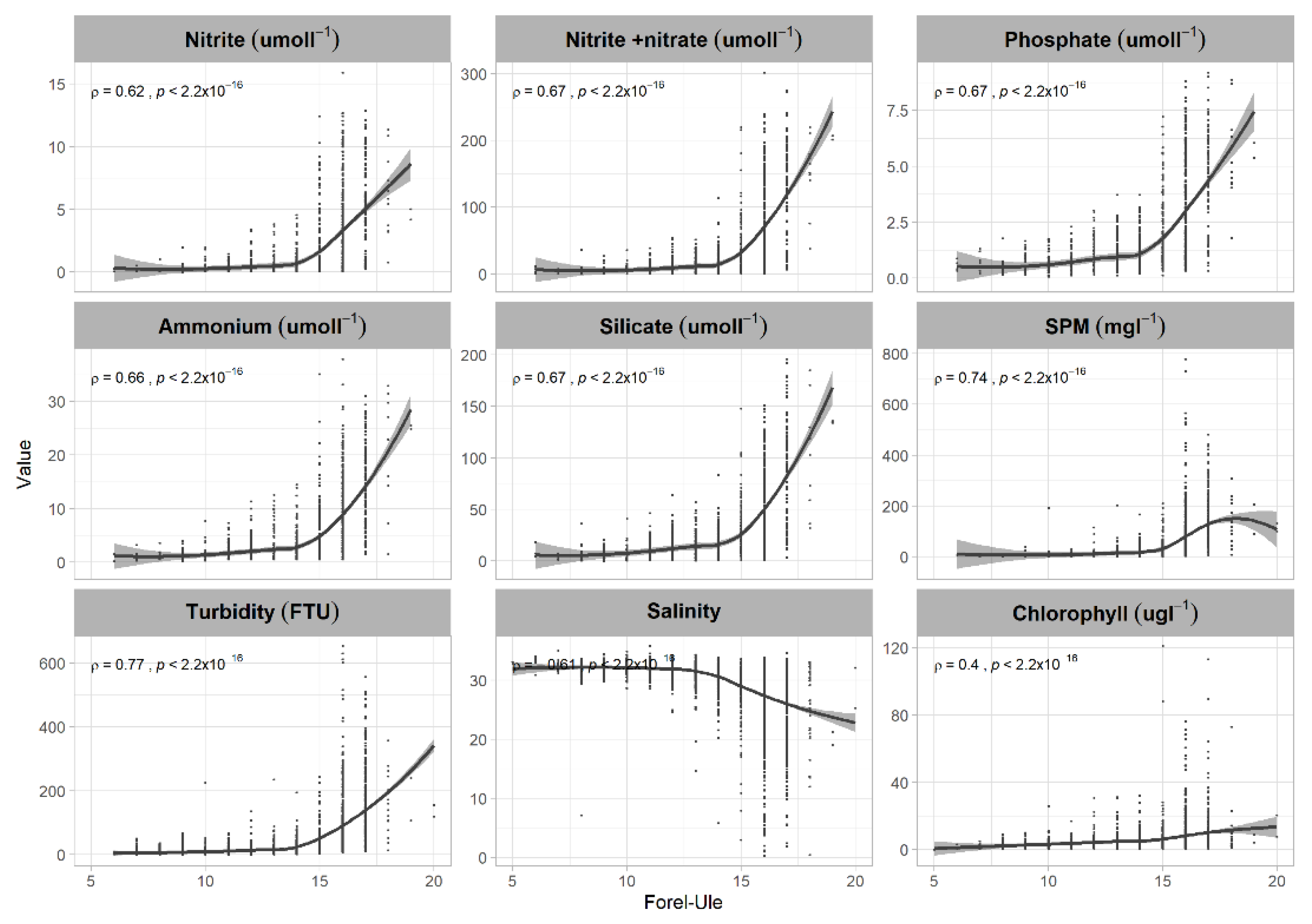
3.2. FUI and Water Quality Indicators
3.3. FUI Plume Typology for Water Quality Assessments
4. Discussion
4.1. Water Quality Assessments Based on the Plume Mapping
4.2. Future Work and Application
5. Conclusions
Supplementary Materials
Author Contributions
Funding
Data Availability Statement
Acknowledgments
Conflicts of Interest
References
- UK National Report. River Basin Management Plans: 2015. 2016. Available online: https://www.gov.uk/government/collections/river-basin-management-plans-2015 (accessed on 18 October 2021).
- Greenwood, N.; Devlin, M.J.; Best, M.; Fronkova, L.; Graves, C.A.; Milligan, A.; Barry, J.; Van Leeuwen, S.M. Utilizing Eutrophication Assessment Directives from Transitional to Marine Systems in the Thames Estuary and Liverpool Bay, UK. Front. Mar. Sci. 2019, 6, 116. [Google Scholar] [CrossRef]
- Foden, J.; Sivyer, D.B.; Mills, D.K.; Devlin, M.J. Spatial and Temporal Distribution of Chromophoric Dissolved Organic Matter (CDOM) Fluorescence and Its Contribution to Light Attenuation in UK Waterbodies. Estuar. Coast. Shelf Sci. 2008, 79, 707–717. [Google Scholar] [CrossRef]
- UK National Report. Common Procedure for the Identification of the Eutrophication Status of the UK Maritime Area. 2017. Available online: http://randd.defra.gov.uk/Document.aspx?Document=ME2205_7330_FRP.pdf (accessed on 18 October 2021).
- Garaba, S.P.; Friedrichs, A.; Voß, D.; Zielinski, O. Classifying Natural Waters with the Forel-Ule Colour Index System: Results, Applications, Correlations and Crowdsourcing. Int. J. Environ. Res. Public Health 2015, 12, 16096–16109. [Google Scholar] [CrossRef] [PubMed] [Green Version]
- Van der Woerd, H.J.; Wernand, M.; Peters, M.; Bala, M.; Brochmann, C. True Color Analysis of Natural Waters with SeaWiFS, MODIS, MERIS and OLCI by SNAP. In Proceedings of the Ocean Optics XXIII, Victoria, BC, Canada, 23–28 October 2016. [Google Scholar]
- Van der Woerd, H.J.; Wernand, M.R. Hue-Angle Product for Low to Medium Spatial Resolution Optical Satellite Sensors. Remote Sens. 2018, 10, 180. [Google Scholar] [CrossRef] [Green Version]
- Petus, C.; Collier, C.; Devlin, M.; Rasheed, M.; McKenna, S. Using MODIS Data for Understanding Changes in Seagrass Meadow Health: A Case Study in the Great Barrier Reef (Australia). Mar. Environ. Res. 2014, 98, 68–85. [Google Scholar] [CrossRef]
- Petus, C.; Devlin, M.; da Silva, E.T.; Lewis, S.; Waterhouse, J.; Wenger, A.; Bainbridge, Z.; Tracey, D. Defining Wet Season Water Quality Target Concentrations for Ecosystem Conservation Using Empirical Light Attenuation Models: A Case Study in the Great Barrier Reef (Australia). J. Environ. Manag. 2018, 213, 451–466. [Google Scholar] [CrossRef]
- Petus, C.; da Silva, E.T.; Devlin, M.; Wenger, A.S.; Álvarez-Romero, J.G. Using MODIS Data for Mapping of Water Types within River Plumes in the Great Barrier Reef, Australia: Towards the Production of River Plume Risk Maps for Reef and Seagrass Ecosystems. J. Environ. Manag. 2014, 137, 163–177. [Google Scholar] [CrossRef] [Green Version]
- Petus, C.; Waterhouse, J.; Lewis, S.; Vacher, M.; Tracey, D.; Devlin, M. A Flood of Information: Using Sentinel-3 Water Colour Products to Assure Continuity in the Monitoring of Water Quality Trends in the Great Barrier Reef (Australia). J. Environ. Manag. 2019, 248, 109255. [Google Scholar] [CrossRef]
- Devlin, M.J.; Petus, C.; Da Silva, E.; Tracey, D.; Wolff, N.H.; Waterhouse, J.; Brodie, J. Water Quality and River Plume Monitoring in the Great Barrier Reef: An Overview of Methods Based on Ocean Colour Satellite Data. Remote Sens. 2015, 7, 12909–12941. [Google Scholar] [CrossRef] [Green Version]
- Petus, C.; Devlin, M.; Thompson, A.; McKenzie, L.; Teixeira da Silva, E.; Collier, C.; Tracey, D.; Martin, K. Estimating the Exposure of Coral Reefs and Seagrass Meadows to Land-Sourced Contaminants in River Flood Plumes of the Great Barrier Reef: Validating a Simple Satellite Risk Framework with Environmental Data. Remote Sens. 2016, 8, 210. [Google Scholar] [CrossRef] [Green Version]
- Waterhouse, J.; Gruber, R.; Logan, M.; Petus, C.; Howley, C.; Lewis, S.; Tracey, D.; James, C.; Mellors, J.; Tonin, H.; et al. Marine Monitoring Program: Annual Report for Inshore Water Quality Monitoring 2019–20; Great Barrier Reef Marine Park Authority: Townsville, Australia, 2021. [Google Scholar]
- Forel, F. Couleur de L’Eau in Optique, Le Léman. Monographie Limnologique, 2nd ed.; Slatkins: Genève, Switzerland, 1895. [Google Scholar]
- Ule, W. Die Bestimmung der Wasserfarbe in Den Seen. Kleinere Mittheilungen. Dr. A. Petermanns Mittheilungen Aus Justus Perthes Geographischer Anstalt; Justus Perthes: Gotha, Germany, 1892; pp. 70–71. [Google Scholar]
- Cie, C. Commission International de l’Eclairage Proceedings 1931; Cambridge University: Cambridge, UK, 1932. [Google Scholar]
- Novoa, S.; Wernand, M.; Van der Woerd, H. The Forel-Ule Scale Revisited Spectrally: Preparation Protocol, Transmission Measurements and Chromaticity. J. Eur. Opt. Soc. Rapid Publ. 2013, 8, 13057. [Google Scholar] [CrossRef] [Green Version]
- Woerd, H.J.; Wernand, M.R. True Colour Classification of Natural Waters with Medium-Spectral Resolution Satellites: SeaWiFS, MODIS, MERIS and OLCI. Sensors 2015, 15, 25663–25680. [Google Scholar] [CrossRef] [PubMed] [Green Version]
- Pitarch, J.; van der Woerd, H.J.; Brewin, R.J.; Zielinski, O. Optical Properties of Forel-Ule Water Types Deduced from 15 Years of Global Satellite Ocean Color Observations. Remote Sens. Environ. 2019, 231, 111249. [Google Scholar] [CrossRef]
- Busch, J.A.; Price, I.; Jeansou, E.; Zielinski, O.; van der Woerd, H.J. Citizens and Satellites: Assessment of Phytoplankton Dynamics in a NW Mediterranean Aquaculture Zone. Int. J. Appl. Earth Obs. Geoinf. 2016, 47, 40–49. [Google Scholar] [CrossRef]
- Wernand, M.; Hommersom, A.; van der Woerd, H.J. MERIS-Based Ocean Colour Classification with the Discrete Forel–Ule Scale. Ocean Sci. 2013, 9, 477–487. [Google Scholar] [CrossRef] [Green Version]
- EyeOnWater. NIOZ, Veerder, MARIS and Citclops Project Partners. Available online: https://www.eyeonwater.org/apps/eyeonwater-colour (accessed on 24 January 2022).
- Novoa, S.; Wernand, M.; van der Woerd, H.J. WACODI: A Generic Algorithm to Derive the Intrinsic Color of Natural Waters from Digital Images. Limnol. Oceanogr. Methods 2015, 13, 697–711. [Google Scholar] [CrossRef] [Green Version]
- Garaba, S.P.; Voß, D.; Zielinski, O. Physical, Bio-Optical State and Correlations in North–Western European Shelf Seas. Remote Sens. 2014, 6, 5042–5066. [Google Scholar] [CrossRef] [Green Version]
- Wooldridge, S.A. Water Quality and Coral Bleaching Thresholds: Formalising the Linkage for the Inshore Reefs of the Great Barrier Reef, Australia. Mar. Pollut. Bull. 2009, 58, 745–751. [Google Scholar] [CrossRef]
- Wooldridge, S.A.; Done, T.J. Improved Water Quality Can Ameliorate Effects of Climate Change on Corals. Ecol. Appl. 2009, 19, 1492–1499. [Google Scholar] [CrossRef]
- McKenzie, L.; Collier, C.; Waycott, M.; Unsworth, R.; Yoshida, R.; Smith, N. Monitoring Inshore Seagrasses of the GBR and Responses to Water Quality. In Proceedings of the 12th International Coral Reef Symposium, Cairns, Australia, 9–13 July 2012. [Google Scholar]
- Collier, C.; Waycott, M.; McKenzie, L. Light Thresholds Derived from Seagrass Loss in the Coastal Zone of the Northern Great Barrier Reef, Australia. Ecol. Indic. 2012, 23, 211–219. [Google Scholar] [CrossRef]
- Unsworth, R.K.; Collier, C.J.; Waycott, M.; Mckenzie, L.J.; Cullen-Unsworth, L.C. A Framework for the Resilience of Seagrass Ecosystems. Mar. Pollut. Bull. 2015, 100, 34–46. [Google Scholar] [CrossRef] [PubMed] [Green Version]
- Polton, J.A.; Palmer, M.R.; Howarth, M.J. Physical and Dynamical Oceanography of Liverpool Bay. Ocean Dyn. 2011, 61, 1421. [Google Scholar] [CrossRef]
- Krausova, A.; Vargas-Silva, C. North East: Census Profile 2013. Available online: http://migrationobservatory.ox.ac.uk/wp-content/uploads/2016/04/CensusProfile-North_East.pdf (accessed on 18 December 2021).
- Turner, G. Summary Statistics for North Wales Region: 2020; Welsh Government: Welsh, UK, 2020.
- Department for Environment, Food and Rural Affairs. Defra Statistics: Agricultural Facts England Regional Profiles; Department for Environment, Food and Rural Affairs: London, UK, 2021.
- Greenwood, N.; Hydes, D.J.; Mahaffey, C.; Wither, A.; Barry, J.; Sivyer, D.B.; Pearce, D.J.; Hartman, S.E.; Andres, O.; Lees, H.E. Spatial and Temporal Variability in Nutrient Concentrations in Liverpool Bay, a Temperate Latitude Region of Freshwater Influence. Ocean Dyn. 2011, 61, 2181–2199. [Google Scholar] [CrossRef]
- Devlin, M.J.; Barry, J.; Mills, D.K.; Gowen, R.J.; Foden, J.; Sivyer, D.; Greenwood, N.; Pearce, D.; Tett, P. Estimating the Diffuse Attenuation Coefficient from Optically Active Constituents in UK Marine Waters. Estuar. Coast. Shelf Sci. 2009, 82, 73–83. [Google Scholar] [CrossRef] [Green Version]
- JNCC. Liverpool Bay/Bae Lerpwl SPA. 2020. Available online: https://jncc.gov.uk/our-work/liverpool-bay-spa/ (accessed on 5 February 2022).
- Moore, A.B.; Bater, R.; Lincoln, H.; Robins, P.; Simpson, S.J.; Brewin, J.; Cann, R.; Chapman, T.; Delargy, A.; Heney, C.; et al. Bass and Ray Ecology in Liverpool Bay. 2020. Available online: https://www.nw-ifca.gov.uk/app/uploads/Agenda-Item-12-Annex-A-Bass_ray_ecology_Liverpool_Bay_3.1_Final.pdf (accessed on 10 February 2022).
- Marine Management Organisation (MMO). Biodiversity, Habitats, Flora and Fauna-Protected Sites and Species; MMO: Newcastle, UK, 2016. [Google Scholar]
- European Space (ESA). Sentinel-3 OLCI User Guide; European Space Agency (ESA): Paris, France, 2018; Available online: https://earth.esa.int/eogateway/documents/20142/1564943/Sentinel-3-OLCI-Marine-User-Handbook.pdf (accessed on 15 January 2022).
- Wyszecki, G.; Stiles, W.S. Colour Science: Concepts and Methods, Quantitative Data and Formulae; John Wiley & Sons: New York, NY, USA, 1982. [Google Scholar]
- Pitarch, J.; Bellacicco, M.; Marullo, S.; Van Der Woerd, H.J. Global Maps of Forel–Ule Index, Hue Angle and Secchi Disk Depth Derived from 21 Years of Monthly ESA Ocean Colour Climate Change Initiative Data. Earth Syst. Sci. Data 2021, 13, 481–490. [Google Scholar] [CrossRef]
- Seneviratne, S.; Nicholls, N.; Easterling, D.; Goodess, C.; Kanae, S.; Kossin, J.; Luo, Y.; Marengo, J.; McInnes, K.; Rahimi, M.; et al. Changes in Climate Extremes and Their Impacts on the Natural Physical Environment. Acad. Commons 2012, 109–230. [Google Scholar] [CrossRef]
- Thewes, D.; Stanev, E.; Zielinski, O. The North Sea Light Climate: Analysis of Observations and Numerical Simulations. J. Geophys. Res. Ocean. 2021, 126, e2021JC017697. [Google Scholar] [CrossRef]
- Wollschläger, J.; Neale, P.J.; North, R.L.; Striebel, M.; Zielinski, O. Climate Change and Light in Aquatic Ecosystems: Variability & Ecological Consequences. Front. Mar. Sci. 2021, 8, 506. [Google Scholar]
- Opdal, A.F.; Lindemann, C.; Aksnes, D.L. Centennial Decline in North Sea Water Clarity Causes Strong Delay in Phytoplankton Bloom Timing. Glob. Chang. Biol. 2019, 25, 3946–3953. [Google Scholar] [CrossRef] [Green Version]
- Brodie, J.; Waterhouse, J.; Maynard, J.; Bennett, J.; Furnas, M.; Devlin, M.; Lewis, S.; Collier, C.; Schaffelke, B.; Fabricius, K.; et al. Assessment of the Relative Risk of Water Quality to Ecosystems of the Great Barrier Reef. A Report to the Department of the Environment and Heritage Protection, Queensland Government, Brisbane-Report 13/28. 2013. Available online: https://www.researchgate.net/publication/285590901_Assessment_of_the_relative_risk_of_water_quality_to_ecosystems_of_the_Great_Barrier_Reef_A_report_to_the_Department_of_the_Environment_and_Heritage_Protection_Queensland_Government_Brisbane_-_Report_1 (accessed on 10 January 2022).


| Source | Water Type (Classes) | FUI | Description |
|---|---|---|---|
| Petus et al., 2019 [11] | Primary | ≥10 | High concentration of phytoplankton, nutrients, sediments and decreased light attenuation |
| Secondary | 6–9 | Dominated by algae, but increased dissolved organic material and some sediment | |
| Tertiary | 4–5 | High light penetration | |
| Marine | 1–3 | High light penetration | |
| Citclops (http://www.citclops.eu/home, accessed on 1 April 2020) | Estuaries | 18–21 | Extremely high concentration of humic acids typical for rivers and Estuaries |
| Near-shore | 14–17 | High nutrient and phytoplankton, increased sediment and dissolved organic material typical for Coastal waters | |
| Coastal | 10–13 | Increased nutrient and phytoplankton, some minerals and dissolved organic material | |
| Open Sea | 1–9 | Dominated by microscopic algae, some sediment might be present but typically the Open Sea |
| Year | Average | Max | Min | STD | Average Dry Season | Average Wet Season | Average Mixed Season |
|---|---|---|---|---|---|---|---|
| 2017 | 2336 | 2915 | 1807 | 306 | 2130 | 2442 | 2435 |
| 2018 | 2231 | 3290 | 1407 | 586 | 1707 | 2799 | 2187 |
| 2019 | 2273 | 3640 | 1493 | 682 | 1625 | 3006 | 2187 |
| 2020 | 2091 | 3596 | 1333 | 628 | 1581 | 2695 | 1998 |
Publisher’s Note: MDPI stays neutral with regard to jurisdictional claims in published maps and institutional affiliations. |
© 2022 by the authors. Licensee MDPI, Basel, Switzerland. This article is an open access article distributed under the terms and conditions of the Creative Commons Attribution (CC BY) license (https://creativecommons.org/licenses/by/4.0/).
Share and Cite
Fronkova, L.; Greenwood, N.; Martinez, R.; Graham, J.A.; Harrod, R.; Graves, C.A.; Devlin, M.J.; Petus, C. Can Forel–Ule Index Act as a Proxy of Water Quality in Temperate Waters? Application of Plume Mapping in Liverpool Bay, UK. Remote Sens. 2022, 14, 2375. https://0-doi-org.brum.beds.ac.uk/10.3390/rs14102375
Fronkova L, Greenwood N, Martinez R, Graham JA, Harrod R, Graves CA, Devlin MJ, Petus C. Can Forel–Ule Index Act as a Proxy of Water Quality in Temperate Waters? Application of Plume Mapping in Liverpool Bay, UK. Remote Sensing. 2022; 14(10):2375. https://0-doi-org.brum.beds.ac.uk/10.3390/rs14102375
Chicago/Turabian StyleFronkova, Lenka, Naomi Greenwood, Roi Martinez, Jennifer A. Graham, Richard Harrod, Carolyn A. Graves, Michelle J. Devlin, and Caroline Petus. 2022. "Can Forel–Ule Index Act as a Proxy of Water Quality in Temperate Waters? Application of Plume Mapping in Liverpool Bay, UK" Remote Sensing 14, no. 10: 2375. https://0-doi-org.brum.beds.ac.uk/10.3390/rs14102375