Surface Water Dynamics from Space: A Round Robin Intercomparison of Using Optical and SAR High-Resolution Satellite Observations for Regional Surface Water Detection

Abstract

Climate change, increasing population and changes in land use are all rapidly driving the need to be able to better understand surface water dynamics. The targets set by the United Nations under Sustainable Development Goal 6 in relation to freshwater ecosystems also make accurate surface water monitoring increasingly vital. However, the last decades have seen a steady decline in in situ hydrological monitoring and the availability of the growing volume of environmental data from free and open satellite systems is increasingly being recognized as an essential tool for largescale monitoring of water resources. The scientific literature holds many promising studies on satellite-based surface-water mapping, but a systematic evaluation has been lacking. Therefore, a round robin exercise was organized to conduct an intercomparison of 14 different satellite-based approaches for monitoring inland surface dynamics with Sentinel-1, Sentinel-2, and Landsat 8 imagery. The objective was to achieve a better understanding of the pros and cons of different sensors and models for surface water detection and monitoring. Results indicate that, while using a single sensor approach (applying either optical or radar satellite data) can provide comprehensive results for very specific localities, a dual sensor approach (combining data from both optical and radar satellites) is the most effective way to undertake largescale national and regional surface water mapping across bioclimatic gradients.

1. Introduction

Water is key to sustainable development, being critical for socioeconomic development, energy and food production, and healthy ecosystems. Today water scarcity affects more than 40 percent of the world’s population and is projected to rise further, exacerbated by climate change [1]. As the global population grows, there is an increasing need to balance the competing demands for water resources and have more efficient ways to manage water supply. The importance of ensuring the availability and sustainable management of water for all has been increasingly addressed in the global political agenda, as seen with the Sixth Sustainable Development Goal (SDG) of the United Nations 2030 Agenda for Sustainable Development [2] and the adoption of an International Decade 2018-2028 for Action on ‘Water for Sustainable Development’ by the UN General Assembly [3]. As the demand for freshwater increases, the importance of monitoring changes in surface waters is gaining more attention, but many countries are still lacking data to monitor the extent of their inland waters and their intra- and interannual changes.

Earth Observation (EO) is an essential source of information, which can complement national hydrometric data and services and support countries to operationally monitor changes to their surface waters. Ever since the launch of the first Earth observation satellites in the early 1970s, the mapping and monitoring of surface water has been a subject that attracts interest from researchers and practitioners in hydrology, environmental conservation, and water resource management. The field has gradually evolved and been incentivized by the steady buildup of long-term archives of global satellite data and computer resources for analyzing those data. A significant breakthrough in the adoption of EO solutions for water=related topics has been the European Commission Joint Research Center’s Global Surface Water Explorer [JRC-GSWE] [4] and the Global Land Analysis and Discovery Group’s Global Surface Water Dynamics [GLAD-GSWD] [5]. Despite these developments and the long track record of related successful case studies on surface water mapping, there is still a lack of clear, robust, efficient, user-oriented methods and guidelines that allow for the use of EO data at scale and on an operational basis for surface water mapping and monitoring.

The mapping of surface water with either optical or Synthetic Aperture Radar (SAR) data has been reviewed in several papers (e.g., [6,7]) and with a series of more recent papers focusing on the combined use of optical and SAR data [8,9,10,11]. This development is directly related to the Sentinel program under the European Copernicus initiative [12] Through the Copernicus Sentinel mission, optical and SAR data in high resolution (10 m) have become globally available free of charge and with a short latency of a few days or less. The next leap in EO-based surface water detection will need to take full advantage of this enhanced observation capacity, which offers unprecedented opportunities to develop robust and cost-effective EO methods to monitor the seasonal and annual variations of surface waters. These EO methods and associated information products can be embedded in national processes for more evidence-based water policies and efficient reporting on the global water agenda. This is why the European Space Agency (ESA) has launched the WorldWater project with a principal aim of strengthening EO capacities in countries to better monitor their inland waterbodies (lakes, reservoirs, rivers, and estuaries) and, consequently, better fulfil their commitments on water resource management and water security in the different water-related global agendas such as the 2030 Agenda on Sustainable Development [2], the 2015 Paris Agreement on climate change [13] and the Sendai Framework for Disaster Risk Reduction [14].

The overarching goal of the WorldWater project is to develop robust and scalable EO solutions for inland surface water monitoring, which can be exploited by a large community of stakeholders involved in water management from local water supplies to national water strategies, including transboundary river basin management plans and global assessment of surface water changes. As part of the project goal, a round robin exercise has been organized to conduct an intercomparison of EO algorithms for surface water detection, using the latest generation of free and open satellite data from Sentinel-1, Sentinel-2, and Landsat 8. The round robin was open to researchers, companies, and other developers of satellite-based algorithms for surface water detection. The precondition for participating in the round robin was a peer-reviewed algorithm for surface water detection based on (or adaptable to) Sentinel-1, Sentinel-2, and/or Landsat 8. Non-peer reviewed algorithms were accepted provided that adequate supplementary documentation and justification could be provided. In this paper, we present the results of the WorldWater round robin intercomparison and use them as the basis for discussing the pros and cons of different approaches to detect and monitor surface waters from Earth observation data. By using various statistical tests, we evaluate the quantitative performance of the individual algorithms and use the findings to draw some qualitative considerations about their performance. The focus is not on the algorithms themselves, as they have already proved themselves (cf. peer-reviewed or in an operational setting), but rather, on the underlying data model, that is, whether the algorithms are relying on single sensor inputs or whether they are using a dual sensor approach. Ideally, the best performing algorithms can provide spatially and temporally consistent timeseries of surface water extent dynamics that meet the user requirements, not only in terms of accuracy but also in terms of transparency, cost, and transferability. The aim is to contribute to the development of a new set of best practices for surface water monitoring, as well as identifying shortfalls and areas of further research.

2. Materials and Methods

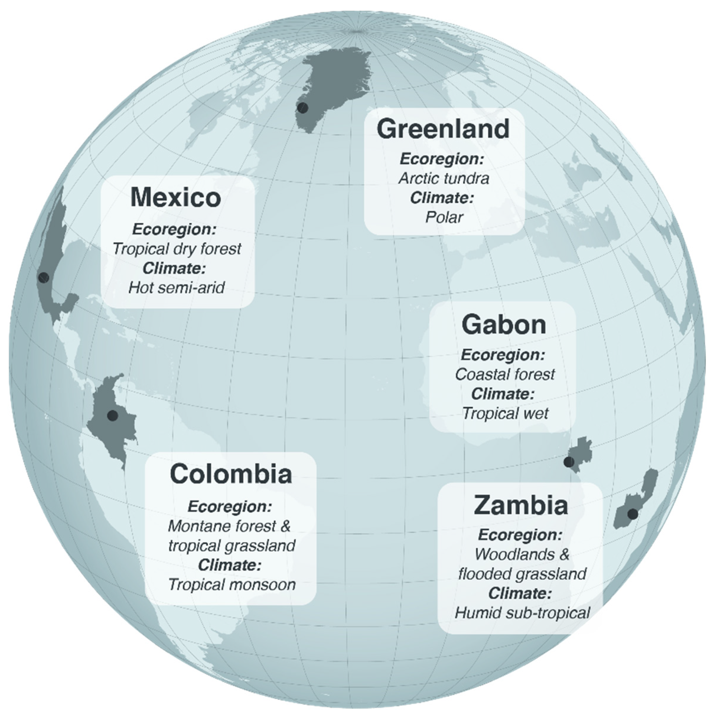
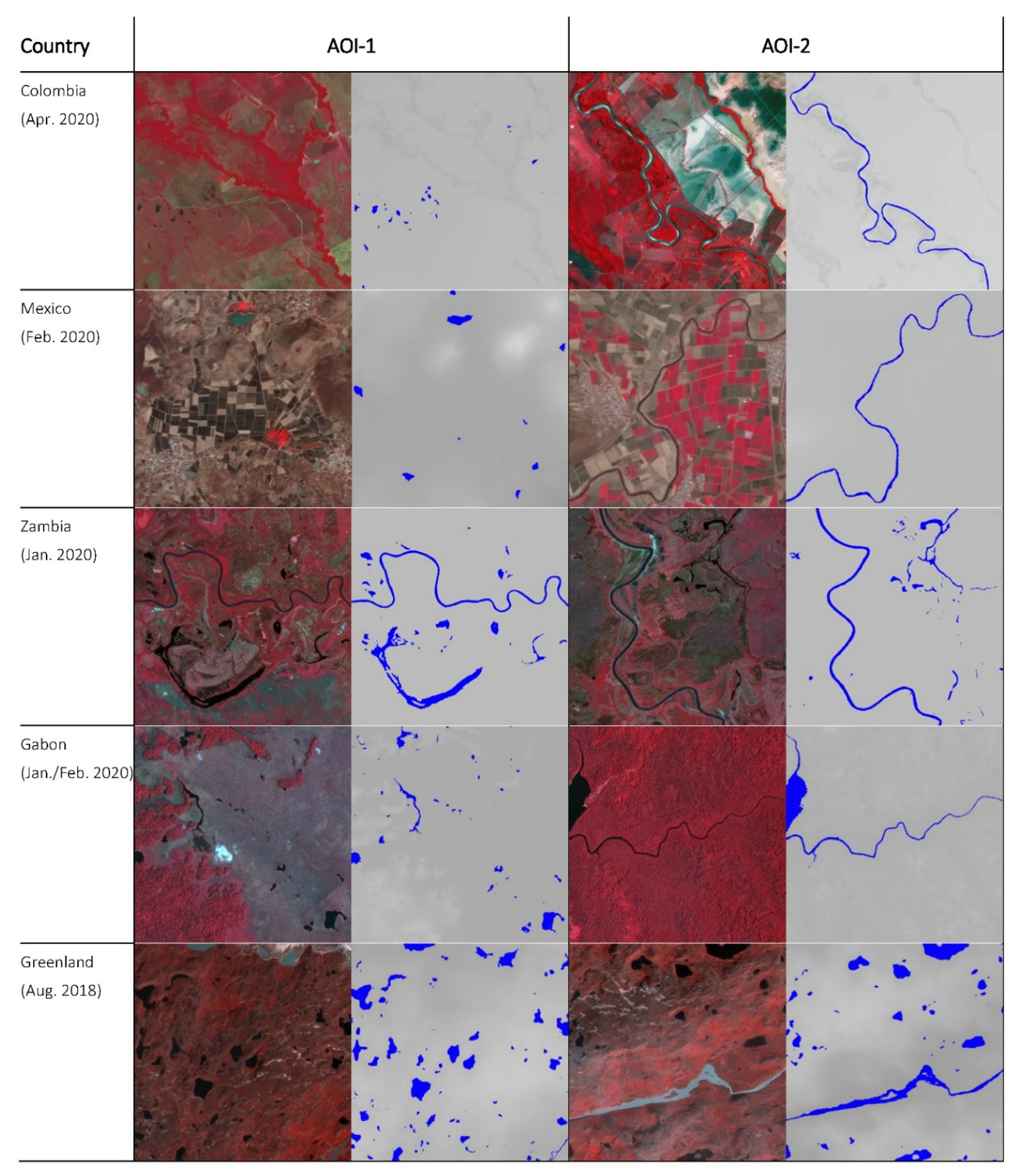
2.1. Test Sites and Input Data

All participants in the round robin were required to produce monthly maps of inland, open surface waters at 10-m spatial resolution for 2 consecutive years over three test sites (100 × 100 km) located in 3 different countries: Colombia, Mexico, and Zambia. Optionally, participants could also submit results for an additional two test sites located in Gabon and Greenland (cf. Figure 1). Test site locations were selected to cover various eco-and climatic regions as well as to include major challenges for EO-based surface water mapping, including sites influenced by topography, clouds, canopy shading, fire scars, urban areas, and regions with permanent low backscatter (e.g., flat and impervious areas, sandy surfaces). The sites also included a diversity of waterbodies ranging from large waterbodies (wind and wave effects) to smaller waterbodies of both a permanent and seasonal nature, as well as waterbodies impacted by water constituents and shallow waters influenced by bottom reflectance. The input datasets, made available to all participants, included all Sentinel 1, Sentinel 2, and Landsat 8 images acquired over the test sites from July 2018 to June 2020. Use of ancillary datasets (such as Digital Elevation Model (DEMs) and a priori surface water maps) were allowed, but under the condition they were publicly available, e.g., the Copernicus DEM [15] and JRC-GSWE [4].

2.2. Surface Water Detection Models

The following sections provide a high-level summary of the fourteen contributions to the round robin intercomparison. Each contribution is referred to as a model in order to emphasis that the focus on the intercomparison was to evaluate the performance of the underlying data models, i.e., whether the surface water detection was based on optical data only (O), SAR data only (S), or integration of both optical and SAR data (O + S).

Model A [O + S] uses a histogram segmentation method to separate imagery from Sentinel-1, Sentinel-2, and Landsat 8 into water and non-water classes [16,17]. Specifically, it carries out edge detection followed by procedures to help obtain a bimodal distribution on which Otsu’s method is carried out to automatically derive an optimal threshold. This model was specifically designed for fast and largescale water detection to assist in flood relief efforts. Similar methods exist that attempt to obtain local thresholds over small sections of each image [18], which can potentially yield more accurate results but at the expense of computational speed. A postprocessing step is applied on the monthly water maps derived separately from optical and SAR imagery, where water pixels are constrained to areas that are hydrologically likely to contain water, with the full timeseries of maps derived from optical imagery included as an additional constraint for the SAR-derived maps. Finally, the optical and SAR-based maps are merged to produce a single water map per month.

Model B [O + S] This surface water detection approach is based on Sentinel-2 imagery as the primary water detection dataset, with the all-weather capabilities of Sentinel-1 SAR imagery being used to “fill-in” cloud-obscured water surfaces. SAR data “in-filling” was restricted to raster cells previously detected as having recorded a surface water content from longer-term data modelling results (circa 2016 and forwards) in order to minimize SAR-generated commission errors in the target month. The water surface modelling procedure is based on a set of decision-tree-generated rules that have been derived from a comprehensive set of water and non-water feature reference points distributed across South Africa. The reference dataset consists of ±60,000 sample points that represent a wide range of seasonal and geographical variations in both water (i.e., turbidity, depth) and non-water surface conditions with potentially similar spectral characteristics, such as burn scars, terrain shadows, and dark, non-vegetated surfaces from both natural and man-made environments. Collectively, these points ensure full representation of all spectral characteristics required in the water detection modelling process. The monthly surface water datasets represent the median surface water extent for that month, rather than the average or (absolute) maximum extent, as a result of the multidate image acquisition date compositing approach used to model water features [19,20].

Model C [O + S] uses a random forest classifier to map surface waterbodies pixel by pixel by taking advantage of the strength of both optical and SAR data in an integrated manner [21]. For optical data, the model relies on a maximum value of the NDWI composite created using both Level-1 and L-2 Sentinel-2 data. The model depends on a minimum radar backscatter intensity, from both VV and VH polarizations, of a composite for sentinel-1 SAR data. Relying composite images minimizes disturbances from clouds, turbidity, and shadows for the optical data and speckles, lake ice, and radar shadows for the SAR data. The model also uses DEM as a feature to remove false positives over a steeper terrain. All the workflows are implemented in Google Earth Engine for ease of transferability and reproducibility.

Model D [O + S] applied a combined histogram-thresholding and edge-detection approach to estimate monthly surface water extent from monthly, cloud-free Sentinel-1, Sentinel-2, and Landsat-8 scenes. Following cloud masking for optical scenes, we applied the Edge-Otsu algorithm to create binary land and water maps for each scene [17,22]. For a complete description and application of the Edge algorithm, see Markert et al., 2020. To initially segment water, histogram-thresholding was performed using the Normalized Difference Water Index (NDWI) index for optical scenes and the VV-median band for SAR scenes within already buffered surface water polygons from Pekel et al., 2016. A second segmentation was applied to full scenes to segment water and non-water, irrespective of initial water polygons. The MERIT DEM [23] was then used to derive a Height Above Nearest Drainage (HAND) model [24] and on regions less than 30 m in height relative to the nearest drainage. Final monthly surface water products combined both optical and SAR water maps by selecting the optical land–water prediction when available, and otherwise selecting the SAR-identified water pixel. Given that cloud-free optical images segment water with higher accuracy than SAR, this approach reduces error during less cloudy periods.

Model E [S] is a fully automated approach that uses dynamic thresholds to classify individual Sentinel-1 scenes. The scene-dependent thresholds to classify water are defined through the use of existing geospatial information of permanent water areas, e.g., data from the Global Surface Water Explorer (GSWE) [4]. The S-1 backscatter values of permanent water areas are derived per scene and are then statistically analyzed by using percentiles to eliminate outliers and a combination of mean and standard deviation to define the individual classification threshold. In opposite to a fixed threshold, this standardized statistical approach allows for the definition of dynamic classification thresholds per scene in order to account for variations in backscatter caused by various factors. The individually classified scenes are then combined to monthly surface water composites, in which false positives (mainly radar shadows) are removed by the use of the Multi-resolution Valley Bottom Flatness (MrVBF) index [25] derived from the Copernicus Digital Elevation Model (DEM). The automated, computationally efficient classification approach has been shown to capture seasonal changes in surface water accurately, but also shows some limitations in non-vegetated sandy areas, in which false positives occur.

Model F [O + S] used combinations of monthly percentile composite images from Sentinel-1 and Normalized Difference Vegetation Index (NDVI), Normalized Difference Water Index (NDWI), Land Surface Water Index (LSWI), Normalized Difference Snow Index (NDSI), red, NIR, and SWIR1 bands from the greenest monthly Sentinel-2 images as covariates for the mapping of monthly surface water extent in Colombia, Mexico, Zambia, and Gabon. For Greenland, covariates from Sentinel-1 were excluded and replaced by monthly minimum NDVI from Sentinel-2 [26]. Training datasets (water–non-water) were generated using a stratified, random sample of points based on Global Surface Water data [4] and visual inspections of spectra profile based on k-means clustering results. Random forest classifier was used for classification.

Model G [S] This approach applies a novel Convolutional Neural Network (CNN) model applied to Sentinel-1 observations to detect surface water. The JRC GSWE product was used as training data, and several finetuning strategies were implemented to improve accuracy of the model in places with complex landcover types. The resulting surface water product has a 10-m spatial resolution, is not impacted by cloud coverage, and can be run in near-real time to detect any surface water changes [27].

Model H [O] uses a thresholding method based on a combination of water indexes (MNDWI > NDVI or MNDWI > EVI) to extract surface water extent from monthly composite Sentinel-2 MSI images. Different from the conventional thresholding method, this algorithm does not need to determine the threshold artificially. To obtain more accurate surface water extent maps, the clouds and cloud shadows pixels, buildup pixels, and snow/ice pixels were removed by auxiliary datasets in preprocessing, and the surface water maps with residual non-water pixels were furtherly denoised in postprocessing. For incomplete monthly surface water extent maps, the surface water frequency map was utilized to fill the gaps caused by clouds and cloud shadows. These methods had been proved effective and accurate in the construction of surface water extent continuous timeseries [28].

Model I [O] uses a multidimensional clustering analysis based on reflectance values and water indices to identify water pixels using optical scenes individually. To achieve high-performance and low memory consumption for high resolution images, this process is applied to a random subsample of the image’s pixels and then coupled with a Naïve Bayes classifier responsible for generalizing the results to the complete scene. The advantage of using an unsupervised approach such as clustering is that the water pixels group is identified automatically by comparing it to other clusters (targets) in the scene. Therefore, the algorithm doesn’t require ancillary data, pretraining, or any threshold calibration, and it is independent of the sensor and the coverage being analyzed. These ideas make it simple to apply the model to a great variety of conditions [29]. As the original algorithm was designed for operational use on single scenes, the monthly water surface has been derived by combining subsequent water masks through an upvote logic that considers as water those pixels that received at least two votes.

Model J [S] This model is based on an unsupervised k-means-clustering algorithm and aims to extract monthly inland waterbody extents over wide areas using multitemporal Sentinel-1 SAR data. To account for slope-induced backscatter differences caused by hills and mountains, due to the slanted acquisition geometry of SAR systems, the model included a radiometric terrain correction, as this step is not applied in the standard Sentinel-1 preprocessing chain. Moreover, the methodology added a multitemporal speckle noise filter which provides better results than a spatial filter applied independently to each SAR image. Seed points for the k-means model are then retrieved by randomly sampling the water layer of the ESA CCI GlobCover Land Cover map [30]. Each sample is represented by a set of temporal features suitable for water characterization in SAR data, such as the mean backscattering value, the maximum value, minimum value, and four “quarter composites” obtained by averaging in time all the Sentinel-1 acquisitions available within each quarter of a year. After the k-means clustering, applied with k = 4, the water cluster is selected by considering a majority voting procedure within the multi-polygon water boundaries of the GlobCover map. Since it is based on SAR data, the methodology can be applied in every weather and lighting condition. Being an unsupervised technique, it is quick, robust, and can be applied automatically over any region of the World [31].

Model L [O] uses the simple yet robust band ratio Normalized Difference Vegetation Index (NDVI) on Sentinel-2 images, screened with the cloud mask processor available in ESA’s SNAP software. Despite the rather simplistic nature of the NDVI band ratio algorithm, results reported in other studies of this type are encouraging (e.g., [26]). Furthermore, the aim of choosing this approach was to test the application of simple and fast algorithms for processing large amounts of images in a short time. We implemented the processing on the Web Advanced Space Developer Interface (WASDI) to process all images without the need for downloading large data quantities on a personal computer [32].

Model M [O + S] uses an efficient and opensource supervised Random Forest classifier system based on Geographic Object-Based Image Analysis (GEOBIA) [33]. It relies on two main components, which are feature extraction based on attribute profiles and a semi-supervised classification using a Random Forest Algorithm. The first step consists of computing features based on Sentinel-2 L1C without cloud detection (MNDWI) and DEM (SRTM or ArcticDEM for Greenland) and extraction of spatial features (object area). The ground truths are automatically extracted from GlobalSurfaceWater data (Pekel et al., 2016). The output from this model is maps of monthly surface water extent and a confidence index. The same automatic system is applied for all 5 test areas.

Model N [O + S] is based on a combination of different image-binarization techniques applied on monthly aggregated Sentinel-1, Sentinel-2, and Landsat-8 imagery. Dynamic, tile-based thresholding [34,35] is conducted on both SAR and optical inputs. In addition, adaptive thresholding [36] and seeded region growing [37] on each initially detected waterbody is performed on the monthly SAR imagery. Finally, fuzzy-logic classification refinement reduces water lookalikes and misclassifications (e.g., radar shadows) from the SAR-based water masks [38,39].

Model O [O + S] uses a multivariate logistic regression model to estimate monthly surface water extent from the combined usages of Sentinel-1, Sentinel-2, and Landsat-8 imagery. Models that rely upon linear distributions are often simpler and generalize well and, therefore, do not require high-quality training labels. Yet, since land–water classification has some nonlinear exceptions, such as clouds, shadows, and snow, the approach integrates logic-based masking to reduce the impact from problematic areas through specific thresholds or basic decision trees. The final approach has proved to be accurate whilst at the same time maintaining computational efficiency and simplicity that facilitates analysis and understanding at scale [8].

2.3. Validation and Evaluation

These water detection models were evaluated individually and in cross-comparison using independent reference data collected from the test sites. A fundamental premise for sound scientific validation is to use reference data of higher quality than the product to be validated. There are two ways to ensure higher quality in the reference data: (i) by using a reference data source with a better resolution than the data used for production (i.e., verification by higher data) and/or (ii) by using a more accurate measurement or interpretation than being used for production (i.e., verification by higher method). A further requirement on the reference data is the ability to provide sufficient spatial and temporal representation to accurately label each unit in the sample; i.e., the ideal reference data are: (i) available for the entire region of interest, (ii) representative of the attribute at the date of interest, and (iii) available at a low cost. The balance between these criteria is often difficult to achieve and why tradeoffs and compromises may be needed when generating the final set of reference data. In the case of the round robin validation, a two-step approach was followed: (i) sample based validation (pixel based) and labelled using the production imagery (verification by higher method) and (ii) object extraction accuracy (area based) and using PlanetScope data as a reference (verification by higher data). The sample-based validation has the advantage of delivering reference data, which can be directly matched (in space and time) to the validation input, whereas the PlanetScope data offer the advantage of better capturing and, hence, better evaluation of smaller and narrower waterbodies/features. Still, the acquisition and interpretation of PlanetScope data is costly, and their representation is therefore restricted in space and time. In a final step, the temporal consistency of the optical, SAR, and dual sensor-mapping approaches were evaluated by comparing the total areal water extent mapped within each test site and across the monthly timeseries. Each validation and evaluation step is described in more detail below.

2.3.1. Sample Based Validation

Stratified random sampling was used to generate reference points over each 100 × 100 km test site and within three strata across the land–water continuum: permanent water, seasonal water, and non-water. The three strata were generated from the JRC-GSWE long-term water occurrence and defined according to the following thresholds: permanent water > 90%; 0% < seasonal water < 90%, and non-water = 0%. In all test sites, the target class “water” is a rare occurrence. In the case of rare occurrences, statistical equations does not allow for proper estimation of sample sizes, but stratified random sampling affords the option to increase the sample size in classes and/or regions that occupy a small proportion of area to thereby help reduce the standard errors of class/region-specific accuracy estimates [40]. It was our aim to ensure a minimum of 50 samples in each stratum, while using subsequent sample size allocations to provide a proportional allocation of samples in better accordance with the actual area of the different strata within each test site. In addition, the expected variance within each stratum was also considered; i.e., the transitional strata are expected to have the highest variance, and why it has a higher sample allocation. Thus, by taking area and expected variance into account, the following sample allocations were applied for the five test sites (cf.

Table 1. Sample size allocations for the 5 test sites used in the round robin.

	Colombia		Gabon		Greenland		Mexico		Zambia
	per month	total	per month	total	per month	total	per month	total	per month	total
Land	140	840	75	450	60	180	140	840	90	540
Transition zone	140	840	150	900	90	270	140	840	190	1140
Water	20	120	60	360	100	300	20	120	40	240
TOTAL	300	1800	285	1710	250	750	300	1800	320	1920

).

In total, 7.980 samples were allocated across the five test sites and six time periods representing every second month of the year 2019 (January, March, May, July, September, November). Each sample point was assigned to be either water or non-water by two independent and experienced interpreters using blind visual interpretations of monthly Sentinel-1 and -2 composites. To harmonize and achieve consistent reference labelling, a standard validation interface was used to ensure interpreters were looking at same area and using the same reference data and the predefined set of classes. In cases where the interpreters disagreed, a quality manager intervened to seek consensus. If consensus could not be agreed upon, the sample was rejected. For each sample we extracted, the respective water classifications and the final set of samples were used to derive standard metrics for accuracy assessments, i.e., overall accuracy (OA), producer accuracy (PA), and user accuracy (UA). For this analysis, all pixels in the individual round robin classifications not classified as water were considered to be non-water; i.e., the non-water class also included pixels being masked (e.g., due to clouds).

2.3.2. Object Extraction Accuracy

Traditionally, stratified point sampling will, in most instances, under-sample Small Waterbodies (SWB) simply because SWBs only represent a fraction of the total water area, even though they may by far exceed the larger waterbodies in numbers [41]. To deal with the issue of SWBs, we complemented the more conventional stratification, sampling, and confusion matrix-type accuracy assessments with an evaluation of object extraction accuracy based on area-based accuracy metrics and the use of higher spatial resolution but single date (i.e., time-limited) PlanetScope data. An independent reference dataset was created from the classification and interpretation of imagery from Planet. The acquired data was PlanetScope Level 3B (Ortho Scene Products) in 3-m spatial resolution and with 4 spectral bands (RGB, NIR) (https://www.planet.com/products/planet-imagery/, accessed on 10 January 2022). The PlanetScope data was acquired within the coverage of each of the test sites and for two areas of approximately 25 km². The exact coverage was determined by size and type of waterbodies, i.e., covering areas with small waterbodies relative to the test site in general and representing both lakes/reservoirs and streams/rivers. For each PlanetScope coverage, we applied a supervised Gradient Boosting (lightGBM) algorithm [42] to generate water masks using the convolution layers derived from spatial filtering of Planet imagery as the explanatory variables and manually derived training samples for water and land (cf. non-water) as the response variable. The Gradient Boosting typically involved a couple of iterations to optimize results, and before finalization, all water masks were manually checked and corrected to ensure high quality. Once analyzed, the PlanetScope data was used to evaluate the object extraction accuracy of the water classifications derived using Sentinel data.

The accuracy evaluation of object extraction is based on object matching, and we focused on two elements related to this, namely: object matching and area-based accuracy measures [43]. The central idea of object matching is to estimate the maximum overlap area by computing the coincidence degree, $A_{max}$, between two objects.

$$A_{max}=\frac{1}{2}\left(\frac{A_{C,i}{{\displaystyle \cap }}^{ }{A}_{R,j}}{A_{C,i}}+\frac{A_{C,i}{{\displaystyle \cap }}^{ }{A}_{R,j}}{A_{R,j}}\right)$$

where $A_{C,i}$ denotes the area of the ith-evaluated object, $A_{R,j}$ is the area of the jth reference object, and $A_{C,i}{{\displaystyle \cap }}^{ }{A}_{R,j}$ represents the intersection area. For an evaluated object and candidate reference objects, each coincidence degree will be computed. Two objects will be judged as being a matching pair if the area of the coincidence degree is at a maximum, i.e., A_max equals 1.

The maximum overlap object matching is complemented by three area-based accuracy measures (i.e., correctness, completeness, and quality). Correctness $(A_{cor})$ is defined as the ratio of the correctly extracted area $(A_C)$ and the whole extracted area $(A_{DC})$, whereas completeness $(A_{com})$ refers to the ratio of the correctly extracted area to the reference area $(A_{RC})$. The range of correctness and completeness is 0 to 1. If $A_C$ fully corresponds to $A_{DC}$ or $A_{RC}$, then the value is 1. If there is no overlap between $A_C$ and $A_{DC}$ or $A_{RC}$, then the value is 0; correctness and completeness interact. For instance, a large $A_{DC}$ leads to a small correctness value, while a small $A_{RC}$ results in a large completeness value. To amend this issue, the quality $A_{qual}$ is designed to provide a measure of quality by balancing correctness and completeness.

$$A_{qual}=\frac{A_C}{A_{DC}+A_{RC}-A_C}$$

The range of quality is 0 to 1. If the water extraction results are the same as the reference data, then the value is 1. If none of the extracted water area overlaps with the reference area, then the value is 0. The advantage of area-based accuracy measures compared to the sample-based validation relates to the fact that the confusion matrix of the latter depends on total pixel number. In contrast, the evaluation results for two cases using area-based accuracy measures are equivalent because it relies only on the evaluation, and reference objects are independent of the total pixel number.

2.3.3. Temporal Consistency Evaluation

The purpose of temporal consistency evaluation is to identify anomalies in sequences of surface water maps. Sudden decreases in surface water can be due not only to drought and high reservoir release but also clouds and lack of valid observation. Flooding, on the other hand, may cause an increase in surface water, but so could cloud shadows and topographic shading, as well as the impact of low-backscatter areas. More robust water detection algorithms should be able to accurately capture actual water dynamics while minimizing the influence of the other factors.

3. Results

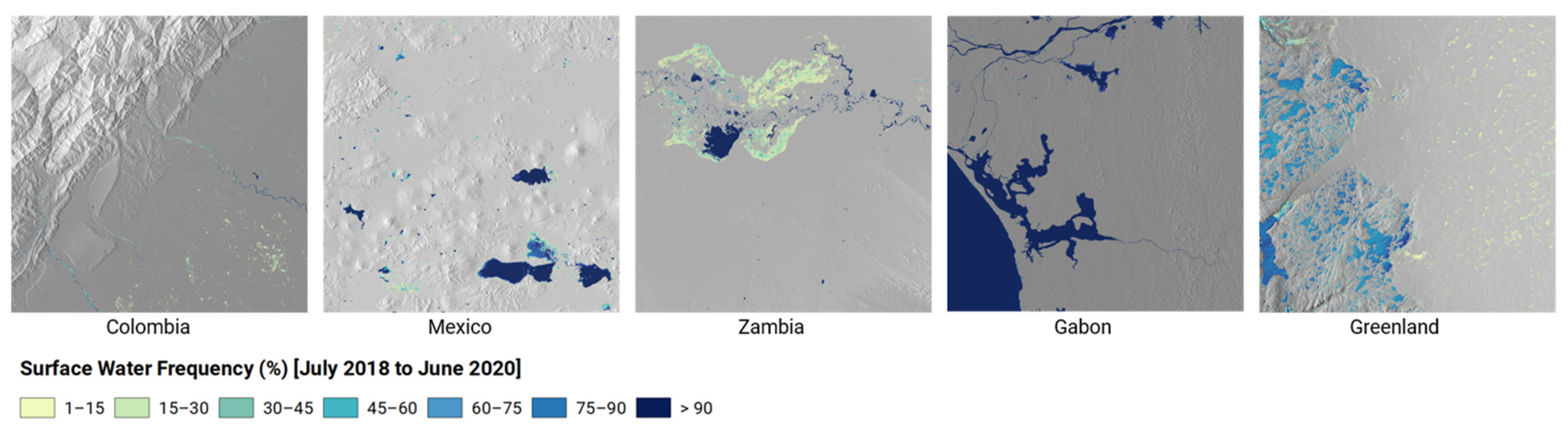
3.1. Water Occurence

The five test sites used for intercomparison represent very different conditions, which can also be inferred by looking at multiannual water occurrence maps for the respective test sites (cf. Figure 2). As explained in Section 2.1, site variability is, on the one hand, dictated by geographic location (i.e., from tropical to arctic, coastal to inland, and lowland to high land) and, on the other hand, by surface water characteristics. The latter is clearly illustrated in the water occurrence maps, which show the differences between test sites in terms of size and type of waterbodies, as well as the relative distribution of permanent and seasonal water (Figure 2). These different characteristics are important to bear in mind when interpreting the validation results, as they will influence the performance of the individual algorithm.

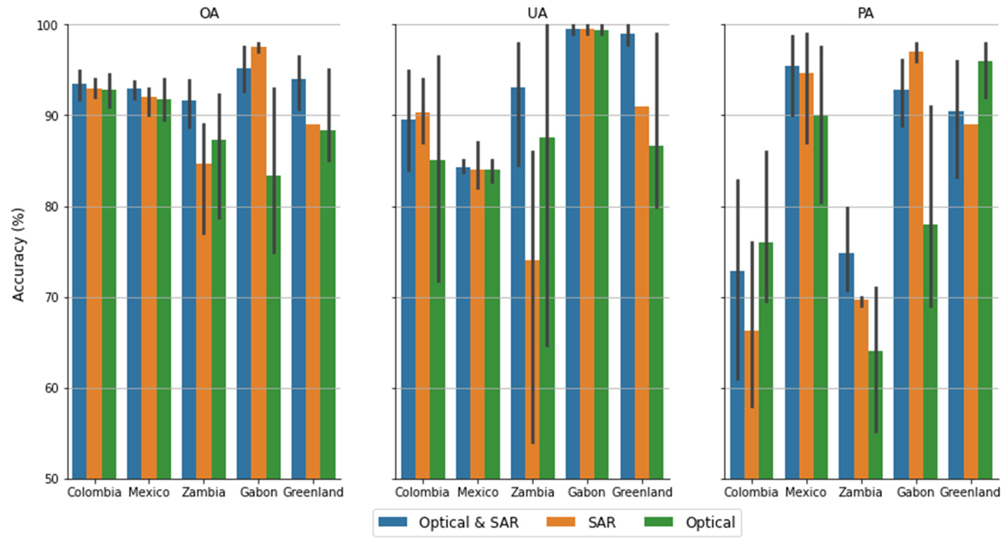
3.2. Sample Based Validation

In Table S1, we provide classification accuracies for the water extraction for all round robin submissions and for each of the three mandatory sites, as well as the optional sites, where relevant. The general performance of all models can be deemed satisfactory, with overall accuracies above or near 90% when looking across the mandatory sites. There is more ambiguity when looking at the performance in terms of user and producer accuracy and at the level of the individual sites.

In Figure 3, the classification accuracies have been grouped (median value) by input data type, i.e., algorithms using both optical and SAR vs. models based on single-sensor inputs (SAR or optical). Figure 3 shows an overall better performance of the combined sensor approach compared to single sensor approaches, although the results are not one-sided when looking at the individual sites or in terms of user and producer accuracies. In Colombia, the combined sensor approach performed best in terms of overall accuracy, but, at the level of UA and PA, the SAR and Optical models, respectively, outperform the combined approach. In Gabon, the SAR approach outperforms the other data models in terms of OA, while in Colombia and Zambia, the optical approach has much higher accuracies for, respectively, PA and UA. In Mexico, OA and UA are almost equal between the data models, but with a noteworthy (+4–5 percentage) drop in producer accuracy for the optical data models compared to the SAR and dual sensor models. The observed differences in UA and PA are closely related to site-specific characteristics. For example, the higher UA accuracies achieved in Gabon and Colombia using SAR are an indication of the benefit SAR adds in a cloud-prone region. In contrast, SAR produces a lower UA in Zambia and Mexico because of commission errors introduced by dry, sandy surfaces. In both Zambia and Mexico, it was also noted that sunglint in certain months caused erroneous cloud masking for certain processors and hence contributed to lowering the PA for the optical data model. In Mexico, the UA for SAR is, however, only marginally lower than for the optical data model, which is impacted by bottom reflectance from shallow waters and turbidity, which both impact the optical properties (cf. spectral signal) of water more than the physical state and, therefore, the sensitivity of SAR backscatter (e.g., roughness). The Zambia site is dominated by the Kafue flats, an extensive wetland ecosystem subject to variable flooding and with a sharp contrast to the surrounding drier landscape, where fire is a major natural factor impacting the landscape. The dynamic nature and many confounding factors (e.g., fires and emergent vegetation) make Zambia a particularly challenging site, and it was also where the dual sensor approach displayed it strongest potential in balancing the individual strengths and weaknesses of optical and SAR data. In Greenland, the topography and light conditions are the main challenges. For optical data, it means higher commission errors (cf. lower UA) due to shading effects and low sun angles. The SAR model is better at dealing with these issues because it works independent of sunlight, and by using ascending and descending SAR scenes, the part of the landscape that can be monitored is increased. Still, the influence of low-backscatter areas (e.g., exposed riverbeds and in snow dominated landscapes) means the SAR data model typically suffers from commission errors and lower PA.

It is important to note that, apart from site-specific characteristics, the UA and PA are also dictated by how individual algorithms have been implemented, e.g., to what extent the individual round robin contributions have favored the importance of commission errors relative to omissions errors. The results will also depend on whether individual scenes are classified and then aggregated to a monthly water map or whether the individual scenes are merged into a monthly composite before water classification. The full accuracy statistics for the individual models is provided as supplementary material (cf. Table S1).

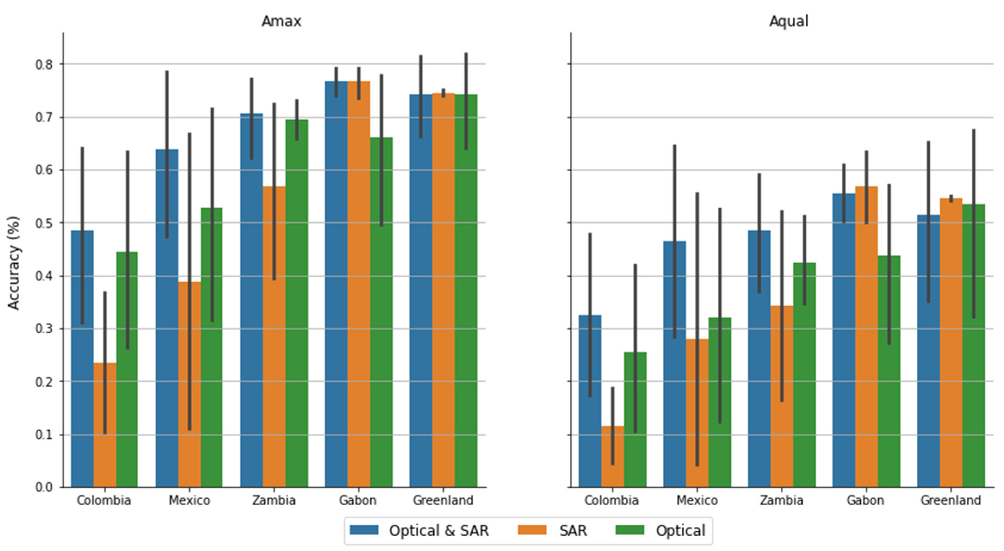
3.3. Object Extraction Accuracy

The 3-m PlanetScope water classification maps used to evaluate object extraction accuracy are shown in Figure 4. Like the full-size test sites, it is important to notice the variability between the sites. Individually, the PlanetScope data represent SWB regions relative to the general water characteristics within their respective test sites, yet, there is variability between sites with, e.g., Zambia having larger waterbodies on average than Colombia.

Table S2 provides an overview of the summary statistics for object extraction accuracy for each of the three mandatory sites, as well as the optional sites, where relevant. There is a large variability between the individual contributions, and yet, with similar tendency across the sites i.e., the algorithms that integrate optical data perform better than those relying solely on SAR (Figure 5). The lowest overall accuracy is in Colombia, and this is also where the difference between the best optical approaches and the best SAR algorithm is greatest (cf. Figure 5). Figure 5 also shows the highest object extraction accuracy is in Zambia, which, together with Greenland, has the largest share of waterbodies within the test sites (cf. Figure 4). It is also noteworthy the optical data model consistently outperforms the SAR data model in all test sites except for Gabon (Figure 5).

The findings from the object extraction accuracy analysis indicate that using or integrating optical data into the water detection algorithm is key to achieving accurate water object definitions. How important depends on the average size of the waterbodies and the surrounding landscape. In Colombia, where the average waterbody size/width is smaller compared to other sites, the difference between the optical algorithms and the SAR-only approaches are the largest. This is explained by the characteristics of the input data, with key spectral water detection bands from Sentinel-2 available only in 10-m spatial resolution, while the true spatial resolution of Sentinel-1 is understood to be closer to 20 × 20 m, although data from the widely used Sentinel-1 Ground Range Detected (GRD) product are delivered with a pixel spacing of 10 × 10 m. There are also some marked differences between the optical algorithms and the SAR only approaches in Mexico, which is likely caused by the dry environment and a landscape dominated by large tracts of dry, sandy surfaces, as well as the associated challenge for SAR-based water detection [44]. In contrast, the difference between optical and SAR is much less pronounced in Zambia and Gabon, which is likely related to the larger average size of the waterbodies (Zambia) and the dense tropical forest landscape causing a stark land–water contrast (Gabon).

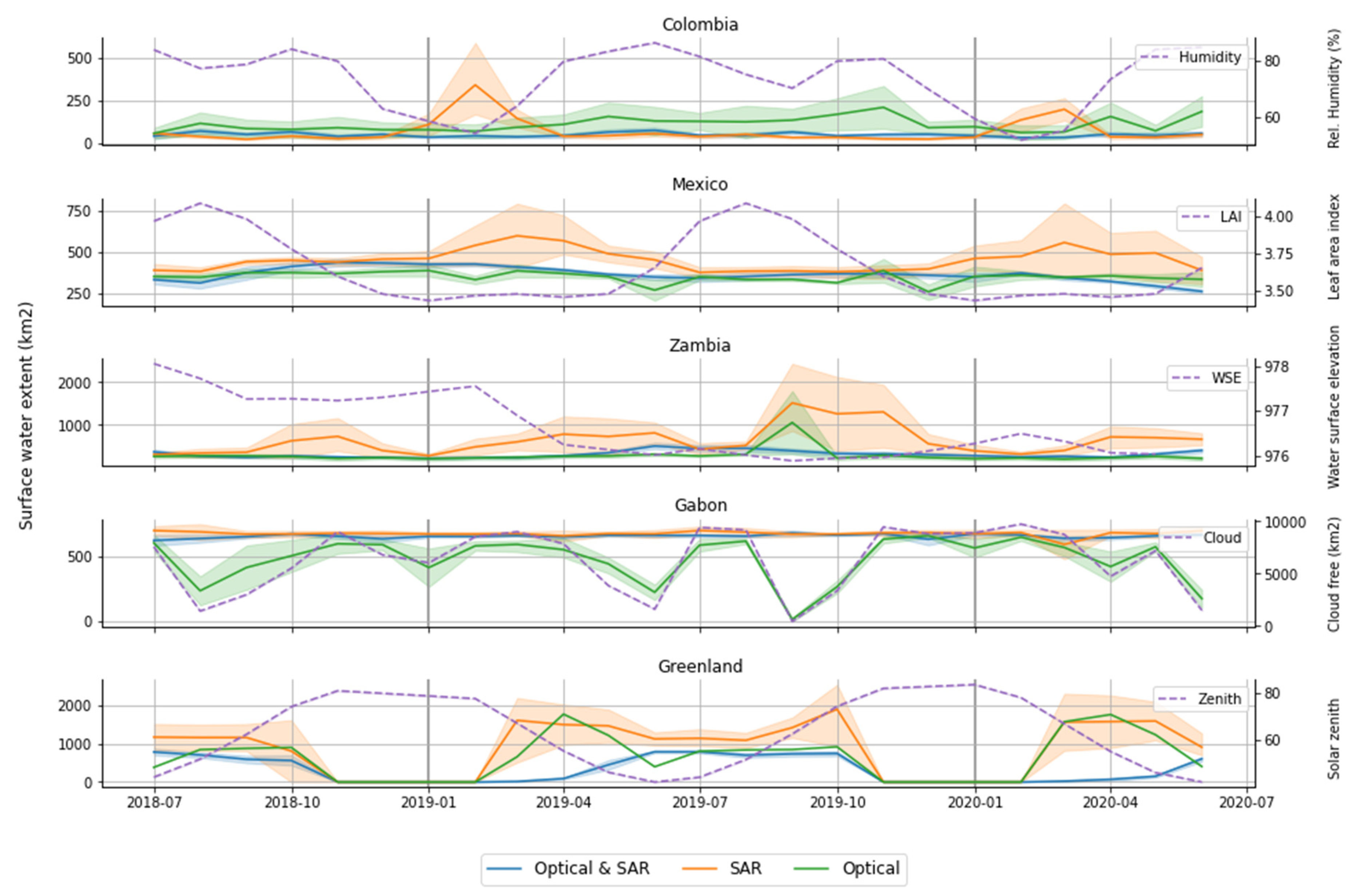
3.4. Temporal Consistency Evaluation

The surface water area (km²) was calculated over each test site and for each month in the 2-year observation period (cf. July 2018 to June 2020). For each test site, the surface water areas were summarized by input data model type, i.e., optical (O), SAR (S), and the fused date model (O + S). In Figure 6, the average surface water area was then plotted against time with indications of variance (i.e., minimum and maximum observed water extent within a given month) and with some key explanatory variables plotted on the secondary axis.

A comparison of the surface water area temporal development curves shows the variance of the fused Optical–SAR-based algorithms are much less than the single sensor solutions both within and between nearby months. If not directly, then at least indirectly, this indicates the fusing algorithms to be more reliable and have less sensitivity to temporary or seasonal phenomena that can impact water detection, including dry/moist conditions, topographic/canopy shading, and clouds.

In Colombia, the pure optical methods, in general, returns a higher surface water area across the entire timeseries. This can be attributed to false positives from topographic shading and ineffective cloud shadow masking, particularly during the humid season. In Mexico, where clouds and topography are less of a problem, there are hardly any noteworthy peaks/dips in the optical development curves. In Colombia and Mexico, the SAR peaks correspond to the dry seasons when the vegetation cover is low, resulting in an increased influence of low backscatter from dry, sandy surfaces.

In Zambia, the variance observed in both the optical and SAR data predictions is most dominant during the 2019 dry season, which was reported as having been one of the worst droughts in Western Zambia in almost 70 years. The exceptionally low water levels during this period indicates that droughts and receding water lines are likely to have an impact on water classifications. The SAR data are challenged by very dry soils, especially in the southern parts of this site, while wildfires represent another challenge for both the optical and SAR data model, as the burn scars can be difficult to separate from water. In optical imagery, burn scars have low reflectance in the near infrared and visible spectrum, and this can lead to spectral confusion with water. As fire also changes the physical and structural characteristics of the vegetated landscape, it also impacts SAR imagery. After a fire, the backscatter decreases strongly [48], and, as a result, the contrast between land and water will be lessened.

In Gabon, the cloud cover percentage over the test site is, on average, 50%, significantly impacting the optical data model, which returns estimates of water extent that strongly correlate with the cloud cover percentage. In contrast, the SAR and fused sensor approach return a much more consistent timeseries, with no apparent sensitivity to the cloud cover percentage.

Finally, in the case of Greenland, the temporal evaluation shows how limited light conditions in spring and fall (before everything freezes) hamper the optical data model. In essence, our evaluation shows the time window to collect optical imagery is short, but also that it can be extended by integration with SAR data. Using a fused data model in Greenland can also help to even out issues generated by a complex topography (e.g., cast shadows in optical imagery and foreshortening and layover effects in the SAR imagery), as indicated in Table S1.

In Figure 6, a large part of the temporal variation is explained by the performance of the individual contributions both between and within the three different sensor models. The dual sensor model has the least variation and, hence, we argue that it is the more robust in dealing with confounding factors. Figure 7 shows the average monthly surface water area statistics for the top three-performing dual sensor models. Figure 7 illustrates quite well the ability of the dual sensor model to provide consistent timeseries information that captures the seasonality of surface water dynamics in each of the test sites. The strongest seasonality is observed in Colombia and Zambia, which are the two test sites with the largest rainfall gradient. In contrast, Mexico and Gabon have less seasonal variation due to very dry (Mexico) and consistently wet (Gabon) conditions. In Greenland, the seasonality is first and foremost dictated by the temperature, i.e., thawing, and increased meltwater starting around April/May and then frost and total freezing once we enter November.

4. Discussion

The round robin evaluation was conducted over a diverse set of test sites that represented landscapes influenced by several of the known challenges for satellite-based surface water mapping, including topography, clouds, dense and inundated vegetation, fire scars, low-backscatter landcovers, low sun angles, as well as snow and ice. The intercomparison of the different round robin contributions across this diverse set of test sites supports the general hypothesis that fusing optical with SAR data produces a more robust mapping of surface water extent dynamics across bioclimatic gradients. Yet, the findings also show that, at individual locations, the single sensor approach can outperform the fused sensor approach. By example SAR data are the better option in heavily clouded regions (cf. Gabon) while optical data are better in dry regions and in capturing smaller waterbodies. As such the round robin provides key insight to the advantage of the strengths of optical and SAR data while also identifying how a fused sensor model can help address their individual shortfalls. Moreover, the evaluation demonstrates that both supervised and unsupervised learning can provide very good results, and while steps for preprocessing and postprocessing are highly relevant to the outcome, they include many variables that are harder to quantify in terms of their individual contributions to the statistical accuracy. Still, there are several crosscutting factors that impact optical and SAR data in various ways, and which underpin why the dual sensor approach, on an overall level, outperforms single sensor approaches.

Both SAR and optical data can struggle in mountainous areas, as steep slopes can lead to shadow issues and image distortions. Orthorectification and radiometric terrain correction using a DEM are the main direct techniques to obtain the relevant geometric and/or signal correction. Yet, such correction can introduce errors, as globally available DEMs have known quality issues [49], although newer DEMs provide gradual improvements [50]. In complex terrain, shadows cast by mountains and hills will appear very dark in optical imagery, which can cause a confusion between topographic shadows and water. This means extra steps should be taken when mapping water extents to make sure the effect of terrain shadow is minimized. While there are specific methods to deal with this in optical imagery [51], SAR imagery can also be used, e.g., to remove water classified in optical imagery if it is consistently mapped as land in SAR (cf. Model A). SAR imagery is not affected by natural sunlight shadows cast by topography. However, radar sensors are side-looking, meaning they view the Earth’s surface from the side of the satellite as it passes by (as opposed to looking directly from above). The side-looking nature of these radar sensors means that they can only see the side of mountains that face their sensors—they cannot see the opposite side of mountains. This is known as radar topographic shadow. Fortunately, radar sensors, such as Sentinel-1, have both ascending and descending orbits, which can collect imagery from east- and west-looking angles. Using ascending and descending imagery together helps to increase the area that can be effectively monitored using radar imagery; however, this does not solve all radar problems related to topography. Areas in deeper canyons and fjords that have a north–south orientation will likely always be in the radar signal shadow, leading to some unavoidable data gaps, and in these cases, sometimes the optical data model can help.

As both SAR and optical data can struggle in mountainous areas, using one sensor to help overcome the other is not always sufficient. Therefore, DEMs are often applied during postprocessing to mask out regions where water formation is unlikely given the topographic conditions, e.g., due to slopes or based on hydrological terrain analysis, such as the Height Above Nearest Drainage (HAND). A range of DEMs have been used for postprocessing, including the Shuttle Radar Topography Mission (SRTM) DEM (e.g., Model B, M), ALOS World 3D-30 m (Model F, J), and Copernicus DEM (Model E, N, O). Although the impact on accuracy is not quantified directly, the use of Copernicus DEM is recommended, not only because Copernicus DEM comes out favorably in statistical evaluations against other DEMs [50], but also because of the reference year (2010–2015), which is newer than SRTM (i.e., 2000) and AW3D30 (2006–2011). In essence, this means the Copernicus DEM is more likely to capture and, hence, avoids masking out newly established reservoirs, which have boomed dramatically in the past few decades [52].

Cloud cover is a major limiting factor affecting the usefulness of optical imagery. However, if clouds and their associated shadows can be effectively masked out from each image, the remaining cloud-free data in each image can be used for accurate water classification, yet the frequency of monitoring will depend on the persistency of the cloud cover. While several algorithms are available for automated cloud masking, (e.g., MAJA, Fmask, CFMask, Tmask, IdePix, Sen2Cor, s2cloudless) none are perfect in separating clear observations from those contaminated with clouds and cloud shadows. Too aggressive cloud masking, and many waterbodies may be missed, while failure to adequately mask cloud shadows will introduce many false positives. Often, making a cloud-free optical image will require some form of image compositing and mosaicking. There are several possible ways to do this, e.g., by using the best available pixel by cloudiness (Model O), or through per-pixel band statistics such as mean/median band reflectances (Model N). Model F applies an NDVI Maximum Value Composite (MVC) procedure, which is effective for providing spatially continuous cloud-free imagery [53]. The MVC has been particularly widely adopted in vegetation studies [54], but, since the MVC emphasizes the vegetation signal, it should be used with care for monitoring water dynamics, as seasonally flooded vegetation may risk being masked. Furthermore, and as illustrated by one contribution, a synthetic timeseries can also be constructed by interpolation and gap-filling using the historical water frequency (cf. Model H). Finally, SAR data can also be used to fill in the “cloud” gaps in the optical imagery. However, even if SAR imagery is not affected by clouds, it is impacted by other issues, which can result in spurious water detection, including speckle noise and permanent low-backscatter regions. The reduction of speckle noise is important to improve the usefulness of SAR imagery. The main purpose of the noise reduction technique is to remove speckle noise while still retaining the important features in the images. Widely adopted speckle filters, such as Lee Sigma or Refined Lee, have proved effective; however, depending on the window kernel size, they may compromise the ability to map smaller water features. Therefore, attention has been drawn to other methods, such as the Gamma Map method (Model A, E) and the use of temporal filtering (e.g., mean, median, or minimum backscatter), as a means to better preserve spatial resolution (cf. Model O, N). The further advantage of using temporal filtering is the ability to also suppress the influence of high winds, which can cause wind-roughened waters that, at specific times, can vanish the contrast between open water and dry surfaces and cause Bragg scattering. With SAR data, it can also be difficult to differentiate water from other surfaces with low backscatter, such as asphalt (parking lots, airports, roads), flat rock, and, in some dry regions, sand surfaces. Long timeseries of backscatter measurements can be used to identify such areas but at the expense of computational efficiency, especially for large areas [55]. Another way is to integrate optical data to reduce potential commission errors caused by permanent low-backscatter areas (cf. Models A and O).

As additional examples, the round robin intercomparisons have also shown how the complementary use of optical and SAR data can help suppress the influence of burn scars and, to an extent, the monitoring period in light-constrained, high-latitude regions.

Aside from the challenges discussed above, there are variables and challenges which could not be fully evaluated. Unresolved issues still circulate around inundated vegetation and how to deal with the cryosphere. As the focus in this study was on open inland waters, neither of these issues was investigated. However, future improvements could be performed through the investigation of L-band SAR sensors, which penetrate vegetation better than C-band SAR data (Sentinel-1) and have potential for mapping flooded areas under vegetated canopies [56,57]. In large parts of the world, lake and river ice is an integral part of annual water dynamics, which is why we also recommend looking at scalable solutions for using optical and SAR data to monitor lake and river ice evolution [58,59] and as complementary information for open surface water dynamics.

Urban environments represent another challenge from the perspective of both optical and SAR data. For optical images, the main issue is building shadows, whereas SAR data may suffer from layover effects caused by tall buildings, as well as corner reflection (cf. double/triple bouncing). Like topography, the urban challenge is often addressed using postprocess masking, which is sensible, especially for large-area applications, as urban areas represent only a fraction of the overall landscape, and the waterbodies associated with the urban environment even less so. In addition, and as new high resolution and freely available urban footprint layers become available [60], urban masking will gradually improve and integrating them as masking layers can help simplify the water mapping solution.

The results and above discussion point to some inherent limitations to mapping surface water when relying solely on either optical or SAR-based instruments. These limitations can be partly mitigated by using both sensors in a fused approach for surface water extent mapping. However, since the fused mapping approach will likely add to complexity, computational effort, transferability, and automation level of the mapping approach, it is important to consider exact needs and objectives before the appropriation of a specific data model.

However, if monitoring is to be conducted in a region with persistent cloud cover, or if the focus is to monitor during the wet–cloudy season, it may be worth considering if adding optical data will bring the necessary improvement to warrant the additional complexity of an operational solution. In other regions, the status of small farm dams may be the most critical information gap in supporting timely information on potential water shortages. In drier regions or during dry spells, where clouds are not an issue, monitoring should rely on optical data only to maximize the spatial resolution. However, where clouds may be an issue, the integration of SAR data will be critical to reliably monitor the status of small farm reservoirs and dams [22,61]. This reiterates that the best practices for surface water monitoring are often reliant on the study domain. In other words, a case-dependent choice of mapping approach will be needed based on certain criteria, such as ecosystem type, seasonality, climate regime, area size, and requirements for the degree of automation. Moreover, as EO technology becomes more widely adopted and mapping approaches evolve, it is further recommended that cross-comparison exercises, as presented in this paper, be repeated periodically to assess advances in surface water mapping.

5. Conclusions

The availability of satellite missions and constellations for environmental monitoring has continued to grow in the past decades, and combined with the advances in technical infrastructures for big data analysis, it is now within the realm of possibility for countries to implement satellite-based surface water monitoring systems. These systems will be vital to supporting more evidence-based planning and management of water resources and provide an ability to efficiently report and act in response to the global water agenda. By evaluating 14 different EO-based models for surface water detection, we show that single sensor approaches can produce accurate and consistent water maps under ideal conditions, and yet, across a range of challenging environments, the synergistic usage of optical and SAR data delivers more accurate and consistent outputs.

The findings in this paper therefore bear some important perspectives for formulating a new best practice where optical and SAR data are used synergistically to achieve the highest accuracy and most consistent results for monitoring surface water dynamics. While accuracy is a critical concern for selecting a surface water detection model, there are other important aspects, including computational efficiency, simplicity, and ease of implementation, which all contribute to increase understanding, maintainability, and potential scalability. In the end, specific working routines, management objectives, and individual user preferences may all contribute to how users will choose to appropriate EO technology for surface water monitoring. At larger scales across diverse ecological gradients, a synergistic approach should be preferred, but at a local scale, SAR data may be preferred for the effective and timely monitoring of water extent and potential emerging floods during cloudy periods, and similar optical data may be preferred to monitor the status of reservoirs and small waterbodies during drought periods and when clouds are not an issue.

Therefore, rather than advocating for a single “best” approach, we recommend flexibility and options to build and/or adapt surface water detection methods that meet individual user needs in terms of management goals, environmental settings, and scale of study, i.e., ensuring users have options for receiving data in multiple formats or from multiple sources, and with the tools necessary to process these data effectively.

The round robin evaluation presented in this paper has shown that EO datasets, methods, and tools for monitoring surface water dynamics are available and successfully applied in various contexts around the globe. The upcoming challenge will be to make the community aware of these tools and, via practical guidance, illustrate how to get started using EO data and tools to support better water resource monitoring, reporting, and management.

References

1. UN. United Nations Sustainable Development Goals: Goal 6: Ensure Access to Water and Sanitation for All. 2020. Available online: https://www.un.org/sustainabledevelopment/water-and-sanitation/ (accessed on 4 April 2022).
2. Long, J. The United Nations’ 2030 Agenda for Sustainable Development and the Impact of the Accounting Industry. Honor. Coll. Theses 2019, 260. Available online: https://digitalcommons.pace.edu/honorscollege_theses/260 (accessed on 4 April 2022).
3. General Assembly of the United Nations. International Decade for Action: Water for Sustainable Development: 2018–2028; UN doc A; RES/71/222 (7 February 2017); United Nations: New York, NY, USA, 2017. [Google Scholar]
4. Pekel, J.F.; Cottam, A.; Gorelick, N.; Belward, A.S. High-resolution mapping of global surface water and its long-term changes. Nature 2016, 540, 418–422. [Google Scholar] [CrossRef] [PubMed]
5. Pickens, A.H.; Hansen, M.C.; Hancher, M.; Stehman, S.V.; Tyukavina, A.; Potapov, P.; Marroquin, B.; Sherani, Z. Mapping and sampling to characterize global inland water dynamics from 1999 to 2018 with full Landsat time-series. Remote Sens. Environ. 2020, 243, 111792. [Google Scholar] [CrossRef]
6. Huang, C.; Chen, Y.; Zhang, S.; Wu, J. Detecting, Extracting, and Monitoring Surface Water From Space Using Optical Sensors: A Review. Rev. Geophys. 2018, 56, 333–360. [Google Scholar] [CrossRef]
7. Brisco, B. Mapping and monitoring surface water and wetlands with synthetic aperture radar. In Remote Sensing of Wetlands: Applications and Advances; Tiner, R.W., Lang, M.W., Klemas, V.V., Eds.; CRC Press: Boca Raton, FL, USA, 2015; pp. 119–136. [Google Scholar]
8. Druce, D.; Xiao, T.; Lei, X.; Guo, T.; Kittel, C.M.M.; Grogan, K.; Tottrup, C. An optical and SAR based fusion approach for mapping surface water dynamics over mainland China. Remote Sens. 2021, 13, 1663. [Google Scholar] [CrossRef]
9. Bioresita, F.; Puissant, A.; Stumpf, A.; Malet, J.-P.P. Fusion of Sentinel-1 and Sentinel-2 image time series for permanent and temporary surface water mapping. Int. J. Remote Sens. 2019, 40, 9026–9049. [Google Scholar] [CrossRef]
10. Markert, K.N.; Chishtie, F.; Anderson, E.R.; Saah, D.; Griffin, R.E. On the merging of optical and SAR satellite imagery for surface water mapping applications. Results Phys. 2018, 9, 275–277. [Google Scholar] [CrossRef]
11. van Leeuwen, B.; Tobak, Z.; Kovács, F. Sentinel-1 and-2 based near real time inland excess water mapping for optimized water management. Sustainability 2020, 12, 2854. [Google Scholar] [CrossRef] [Green Version]
12. Showstack, R. NEWS Sentinel Satellites Initiate New Era in Earth Observation. EOS 2014, 95, 239–240. [Google Scholar] [CrossRef]
13. UNFCCC. Paris Agreement. 2015. Available online: http://unfccc.int/files/essential_background/convention/application/pdf/english_paris_agreement.pdf (accessed on 4 April 2022).
14. UNDRR. Sendai Framework for Disaster Risk Reduction. 2015. Available online: https://www.undrr.org/implementing-sendai-framework/what-sendai-framework (accessed on 4 April 2022).
15. Airbus. Copernicus DEM Product Handbook. 2019. Available online: https://spacedata.copernicus.eu/documents/20126/0/GEO1988-CopernicusDEM-SPE-002_ProductHandbook_I1.00+%281%29.pdf/40b2739a-38d3-2b9f-fe35-1184ccd17694?t=1612269439996 (accessed on 2 March 2021).
16. Donchyts, G.; Schellekens, J.; Winsemius, H.; Eisemann, E.; Van de Giesen, N. A 30 m Resolution Surface Water Mask Including Estimation of Positional and Thematic Differences Using Landsat 8, SRTM and OpenStreetMap: A Case Study in the Murray-Darling Basin, Australia. Remote Sens. 2016, 8, 386. [Google Scholar] [CrossRef] [Green Version]
17. Markert, K.N.; Markert, A.M.; Mayer, T.; Nauman, C.; Haag, A.; Poortinga, A.; Bhandari, B.; Thwal, N.S.; Kunlamai, T.; Chishtie, F.; et al. Comparing Sentinel-1 surface water mapping algorithms and radiometric terrain correction processing in southeast Asia utilizing Google Earth Engine. Remote Sens. 2020, 12, 2469. [Google Scholar] [CrossRef]
18. Chini, M.; Hostache, R.; Giustarini, L.; Matgen, P. A hierarchical split-based approach for parametric thresholding of SAR images: Flood inundation as a test case. IEEE Trans. Geosci. Remote Sens. 2017, 55, 6975–6988. [Google Scholar] [CrossRef]
19. Thompson, M.; Hiestermann, J.; Eady, B.; Hallowes, J. Frankly My Dear I Give a Dam! Or Using Satellite Observation to Determine Water Resource Availability in Catchments. 2018. Available online: http://sbdvc.ekodata.co.za/downloads/SANCIAHS_paper.pdf (accessed on 6 May 2022).
20. Department of Science and Innovation Republic of South Africa. mzansiAmanzi—A Monthly Outlook of Water in South Africa. Available online: https://www.water-southafrica.co.za/ (accessed on 6 May 2022).
21. Wangchuk, S.; Bolch, T. Mapping of glacial lakes using Sentinel-1 and Sentinel-2 data and a random forest classifier: Strengths and challenges. Sci. Remote Sens. 2020, 2, 100008. [Google Scholar] [CrossRef]
22. Vanthof, V.; Kelly, R. Water storage estimation in ungauged small reservoirs with the TanDEM-X DEM and multi-source satellite observations. Remote Sens. Environ. 2019, 235, 111437. [Google Scholar] [CrossRef]
23. Yamazaki, D.; Ikeshima, D.; Neal, J.C.; O’Loughlin, F.; Sampson, C.C.; Kanae, S.; Bates, P.D. MERIT DEM: A new high-accuracy global digital elevation model and its merit to global hydrodynamic modeling. AGU Fall Meet. Abstr. 2017, 2017, H12C-04. [Google Scholar]
24. Nobre, A.D.; Cuartas, L.A.; Hodnett, M.; Rennó, C.D.; Rodrigues, G.; Silveira, A.; Saleska, S. Height Above the Nearest Drainage–a hydrologically relevant new terrain model. J. Hydrol. 2011, 404, 13–29. [Google Scholar] [CrossRef] [Green Version]
25. Gallant, J.C.; Dowling, T.I. A multiresolution index of valley bottom flatness for mapping depositional areas. Water Resour. Res. 2003, 39, 12. [Google Scholar] [CrossRef]
26. Fan, X.; Liu, Y.; Wu, G.; Zhao, X. Compositing the Minimum NDVI for Daily Water Surface Mapping. Remote Sens. 2020, 12, 700. [Google Scholar] [CrossRef] [Green Version]
27. Guzder-Williams, B.; Alemohammad, H. Surface Water Detection from Sentinel-1. In Proceedings of the IEEE International Geoscience and Remote Sensing Symposium IGARSS, Brussels, Belgium, 11–16 July 2021. [Google Scholar]
28. Zhou, H.; Liu, S.; Hu, S.; Mo, X. Retrieving dynamics of the surface water extent in the upper reach of Yellow River. Sci. Total Environ. 2021, 800, 149348. [Google Scholar] [CrossRef]
29. Cordeiro, M.C.R.; Martinez, J.-M.; Peña-Luque, S. Automatic water detection from multidimensional hierarchical clustering for Sentinel-2 images and a comparison with Level 2A processors. Remote Sens. Environ. 2021, 253, 112209. [Google Scholar] [CrossRef]
30. Defourny, P.; Kirches, G.; Brockmann, C.; Boettcher, M.; Peters, M.; Bontemps, S.; Lamarche, C.; Schlerf, M.; Santoro, M. Land cover CCI: Product User Guide Version 2.0. 2017. Available online: http://maps.elie.ucl.ac.be/CCI/viewer/download/ESACCI-LC-Ph2-PUGv2_2.0.pdf (accessed on 4 April 2022).
31. Marzi, D.; Gamba, P. Inland Water Body Mapping Using Multitemporal Sentinel-1 SAR Data. IEEE J. Sel. Top. Appl. Earth Obs. Remote Sens. 2021, 14, 11789–11799. [Google Scholar] [CrossRef]
32. Schumann, G.J.P.; Campanella, P.; Tasso, A.; Giustarini, L.; Matgen, P.; Chini, M.; Hoffmann, L. An Online Platform for Fully-Automated EO Processing Workflows for Developers and End-Users Alike. In Proceedings of the 2021 IEEE International Geoscience and Remote Sensing Symposium IGARSS, Brussels, Belgium, 11–16 July 2021; pp. 8656–8659. [Google Scholar]
33. Merciol, F.; Faucqueur, L.; Damodaran, B.B.; Rémy, P.-Y.; Desclée, B.; Dazin, F.; Lefèvre, S.; Masse, A.; Sannier, C. Geobia at the terapixel scale: Toward efficient mapping of small woody features from heterogeneous vhr scenes. ISPRS Int. J. Geo-Inf. 2019, 8, 46. [Google Scholar] [CrossRef] [Green Version]
34. Ludwig, C.; Walli, A.; Schleicher, C.; Weichselbaum, J.; Riffler, M. A highly automated algorithm for wetland detection using multi-temporal optical satellite data. Remote Sens. Environ. 2019, 224, 333–351. [Google Scholar] [CrossRef]
35. Martinis, S.; Twele, A.; Voigt, S. Towards operational near real-time flood detection using a split-based automatic thresholding procedure on high resolution TerraSAR-X data. Nat. Hazards Earth Syst. Sci. 2009, 9, 303–314. [Google Scholar] [CrossRef]
36. Bradley, D.; Roth, G. Adaptive thresholding using the integral image. J. Graph. Tools 2007, 12, 13–21. [Google Scholar] [CrossRef]
37. Adams, R.; Bischof, L. Seeded region growing. IEEE Trans. Pattern Anal. Mach. Intell. 1994, 16, 641–647. [Google Scholar] [CrossRef] [Green Version]
38. Martinis, S.; Kersten, J.; Twele, A. A fully automated TerraSAR-X based flood service. ISPRS J. Photogramm. Remote Sens. 2015, 104, 203–212. [Google Scholar] [CrossRef]
39. Twele, A.; Cao, W.; Plank, S.; Martinis, S. Sentinel-1-based flood mapping: A fully automated processing chain. Int. J. Remote Sens. 2016, 37, 2990–3004. [Google Scholar] [CrossRef]
40. Olofsson, P.; Foody, G.M.; Herold, M.; Stehman, S.V.; Woodcock, C.E.; Wulder, M.A. Good practices for estimating area and assessing accuracy of land change. Remote Sens. Environ. 2014, 148, 42–57. [Google Scholar] [CrossRef]
41. Downing, J.A.; Prairie, Y.T.; Cole, J.J.; Duarte, C.M.; Tranvik, L.J.; Striegl, R.G.; McDowell, W.H.; Kortelainen, P.; Caraco, N.F.; Melack, J.M. The global abundance and size distribution of lakes, ponds, and impoundments. Limnol. Oceanogr. 2006, 51, 2388–2397. [Google Scholar] [CrossRef] [Green Version]
42. Ke, G.; Meng, Q.; Finley, T.; Wang, T.; Chen, W.; Ma, W.; Ye, Q.; Liu, T.-Y. Lightgbm: A highly efficient gradient boosting decision tree. Adv. Neural Inf. Process. Syst. 2017, 30, 3146–3154. [Google Scholar]
43. Cai, L.; Shi, W.; Miao, Z.; Hao, M. Accuracy assessment measures for object extraction from remote sensing images. Remote Sens. 2018, 10, 303. [Google Scholar] [CrossRef] [Green Version]
44. Martinis, S.; Kuenzer, C.; Wendleder, A.; Huth, J.; Twele, A.; Roth, A.; Dech, S. Comparing four operational SAR-based water and flood detection approaches. Int. J. Remote Sens. 2015, 36, 3519–3543. [Google Scholar] [CrossRef]
45. Climate Data Store. ERA5 Climate Reanalysis. Available online: https://cds.climate.copernicus.eu/ (accessed on 27 March 2022).
46. U.S. Department of Agriculture. Global Reservoirs and Lakes Monitor (G-REALM). Available online: https://ipad.fas.usda.gov/cropexplorer/global_reservoir/ (accessed on 22 March 2022).
47. European Union/ESA/Copernicus/SentinelHub. Sentinel-2: Cloud Probability. Available online: https://developers.google.com/earth-engine/datasets/catalog/COPERNICUS_S2_CLOUD_PROBABILITY#description (accessed on 22 March 2022).
48. Siegert, F.; Ruecker, G. Use of multitemporal ERS-2 SAR images for identification of burned scars in south-east Asian tropical rainforest. Int. J. Remote Sens. 2000, 21, 831–837. [Google Scholar] [CrossRef]
49. Uuemaa, E.; Ahi, S.; Montibeller, B.; Muru, M.; Kmoch, A. Vertical Accuracy of Freely Available Global Digital Elevation Models (ASTER, AW3D30, MERIT, TanDEM-X, SRTM, and NASADEM). Remote Sens. 2020, 12, 3482. [Google Scholar] [CrossRef]
50. Guth, P.L.; Geoffroy, T.M. LiDAR point cloud and ICESat-2 evaluation of 1 second global digital elevation models: Copernicus wins. Trans. GIS 2021, 25, 2245–2261. [Google Scholar] [CrossRef]
51. Tottrup, C. Forest and land cover mapping in a tropical highland region. Photogramm. Eng. Remote Sens. 2007, 73, 1057. [Google Scholar]
52. Zarfl, C.; Lumsdon, A.E.; Berlekamp, J.; Tydecks, L.; Tockner, K. A global boom in hydropower dam construction. Aquat. Sci. 2015, 77, 161–170. [Google Scholar] [CrossRef]
53. Holben, B.N. Characteristics of maximum-value composite images from temporal AVHRR data. Int. J. Remote Sens. 1986, 7, 1417–1434. [Google Scholar] [CrossRef]
54. Pettorelli, N.; Vik, J.O.; Mysterud, A.; Gaillard, J.-M.; Tucker, C.J.; Stenseth, N.C. Using the satellite-derived NDVI to assess ecological responses to environmental change. Trends Ecol. Evol. 2005, 20, 503–510. [Google Scholar] [CrossRef]
55. Schlaffer, S.; Matgen, P.; Hollaus, M.; Wagner, W. Flood detection from multi-temporal SAR data using harmonic analysis and change detection. Int. J. Appl. Earth Obs. Geoinf. 2015, 38, 15–24. [Google Scholar] [CrossRef]
56. Tsyganskaya, V.; Martinis, S.; Marzahn, P.; Ludwig, R. SAR-based detection of flooded vegetation–a review of characteristics and approaches. Int. J. Remote Sens. 2018, 39, 2255–2293. [Google Scholar] [CrossRef]
57. Tsyganskaya, V.; Martinis, S.; Marzahn, P.; Ludwig, R. Detection of temporary flooded vegetation using Sentinel-1 time series data. Remote Sens. 2018, 10, 1286. [Google Scholar] [CrossRef] [Green Version]
58. Wang, X.; Feng, L.; Gibson, L.; Qi, W.; Liu, J.; Zheng, Y.; Tang, J.; Zeng, Z.; Zheng, C. High-Resolution Mapping of Ice Cover Changes in Over 33,000 Lakes Across the North Temperate Zone. Geophys. Res. Lett. 2021, 48, e2021GL095614. [Google Scholar] [CrossRef]
59. Scott, K.A.; Xu, L.; Pour, H.K. Retrieval of ice/water observations from synthetic aperture radar imagery for use in lake ice data assimilation. J. Great Lakes Res. 2020, 46, 1521–1532. [Google Scholar] [CrossRef]
60. Esch, T.; Marconcini, M.; Felbier, A.; Roth, A.; Heldens, W.; Huber, M.; Schwinger, M.; Taubenböck, H.; Müller, A.; Dech, S. Urban footprint processor—Fully automated processing chain generating settlement masks from global data of the TanDEM-X mission. IEEE Geosci. Remote Sens. Lett. 2013, 10, 1617–1621. [Google Scholar] [CrossRef] [Green Version]
61. Perin, V.; Tulbure, M.G.; Gaines, M.D.; Reba, M.L.; Yaeger, M.A. A multi-sensor satellite imagery approach to monitor on-farm reservoirs. Remote Sens. Environ. 2022, 270, 112796. [Google Scholar] [CrossRef]
Figure 1. Location map of the test sites annotated with their dominant eco-region(s).
Remotesensing 14 02410 g001
Figure 2. Examples of surface water frequency maps over the 5 test sites and as derived by Model N.
Remotesensing 14 02410 g002
Figure 3. Accuracy statistics from the WorldWater round robin test sites, individually and overall, summarized by model input data type (OA = Overall Accuracy; UA = User Accuracy; PA = Producer Accuracy).
Remotesensing 14 02410 g003
Figure 4. False colour PlanetScope QuickLooks and associated water classifications for each AOI used in the object-based validation approach (Imagery © 2022 Planet Labs Inc.).
Remotesensing 14 02410 g004
Figure 5. Object accuracy statistics from the WorldWater round robin PlanetScope sites, summarized by country and model input data type.
Remotesensing 14 02410 g005
Figure 6. Monthly surface water area trajectories for the individual test sites and per sensor model. For each test site, corresponding timeseries of the key explanatory variables are equally shown, i.e., the Humidity and Leaf Area Index from the ERA-5 monthly averaged reanalysis data [45], water surface elevation from satellite altimetry [46], solar zenith angle, and cloud cover [47].
Remotesensing 14 02410 g006
Figure 7. Interannual monthly mean surface water area dynamics and uncertainties (98% CI), as captured by the best-performing dual sensor models (i.e., models A, N, and O).
Remotesensing 14 02410 g007