Article

Estimation of Pb Content Using Reflectance Spectroscopy in Farmland Soil near Metal Mines, Central China

1
Shaanxi Key Laboratory of Land Consolidation, School of Land Engineering, Chang’an University, Xi’an 710054, China
2
School of Earth Sciences and Resources, Chang’an University, Xi’an 710054, China
3
Department of Earth and Atmospheric Sciences, University of Alberta, Edmonton, AB T6G2E3, Canada
*
Author to whom correspondence should be addressed.
These authors contributed equally to this work.
Remote Sens. 2022, 14(10), 2420; https://0-doi-org.brum.beds.ac.uk/10.3390/rs14102420
Submission received: 16 March 2022 / Revised: 7 May 2022 / Accepted: 11 May 2022 / Published: 18 May 2022

Abstract

:
The contamination of farmlands with hazardous metals from mining puts the safety of agricultural commodities at risk. For remediation, it is crucial to map the spatial distribution of contaminated soil. Typical sampling-based procedures are time-consuming and labor-intensive. The use of visible, near-infrared, and short-wave infrared reflectance (VNIR-SWIR) spectroscopy to detect soil heavy metal pollution is an alternative. With the aim of investigating a methodology of detecting the most sensitive bands using VNIR-SWIR spectra to find lead (Pb) anomalies in agriculture soil near mining activities, the area in Xiaoqinling Mountain, downstream from a series of active gold mines, was selected to test the feasibility of utilizing VNIR-SWIR spectroscopy to map soil Pb. A total of 115 soil samples were collected for laboratory Pb analysis and spectral measurement. Partial least squares regression (PLSR) was adopted to estimate the soil Pb content by building the prediction model, and the model was optimized by finding the optimal number of bands involved. The spatial distribution of Pb concentration was mapped using the ordinary kriging (OK) interpolation method. This study found that five spectral bands (522 nm, 1668 nm, 2207 nm, 2296 nm, and 2345 nm) were sensitive to soil Pb content. The optimized prediction model’s coefficient of determination (R2), residual prediction deviation (RPD), and root mean square error (RMSE) were 0.711, 1.860, and 0.711 ln(mg/kg), respectively. Additionally, the result of OK interpolation was convincing and accurate (R2 = 0.775, RMSE = 0.328 ln(mg/kg)), comparing maps from estimated and ground truth data. This study proves that it is feasible to use VNIR-SWIR spectral data for in situ estimation of the soil Pb content.

Graphical Abstract

1. Introduction

The impact of heavy metal contamination in ecosystems is a primary concern for modern society. It can reduce soil fertility and crop production because of the concealed, hysteretic, cumulative, and irreversible characteristics of the heavy metal in soil. It poses threats to human health through the food chain, direct ingestion, dermal absorption, and respiratory system [1,2]. Studies have shown that human diseases, including complications of the nerves, bones, blood circulation, endocrine, and immune systems, could be associated with the intake of heavy metals [3]. Mining activity, as one of the major sources of heavy metal contamination in soil [4,5,6], should be monitored dynamically to identify the pollution level of heavy metals; this is critical for policymaking and soil remediation [7].
The conventional strategy for monitoring soil contamination is based on sampling and laboratory analysis of heavy metals in soil samples. This approach yields excellent precision for each sample [8], but spatial accuracy is dependent on the size of the sampling grid (or mapping scale). It is costly and time-consuming to obtain the pollutant distribution map in large areas [6]. The visible, near-infrared, and short-wave infrared reflectance (VNIR-SWIR) spectroscopy technology is a non-destructive approach to quickly determine soil heavy metal contamination quantitatively [6,9]. Previous research demonstrated that reflectance spectra can be used to estimate the distributions of heavy metals in soil, and multivariate analysis can analyze complicated mixes of soil constituents [10,11,12,13]. However, the wavelength and number of sensitive bands for predicting the same soil element are different for each research [14,15,16], and the relationship between the accuracy of the prediction model and the involved spectral features has not been thoroughly studied. In addition, the organic matter, iron oxides, and clay minerals in the soil can adsorb heavy metals and affect the selection of sensitive bands in a particular region, which must therefore be investigated [17,18,19].
The Xiaoqinling Mountain in China is the second-largest gold-bearing area, with over 1000 years of mining history and an extensive research background. It has been found that mining activities in the Xiaoqinling Mountain region have contributed to heavy metal contamination in agricultural soils [20]. Previous studies have found that mines are significant contributors to soil contamination downstream [20,21] and Pb pollution is a critical indicator, while various other contaminants are often correlated to Pb concentration. The soil Pb content is known to be associated with the cation exchange capacity (CEC), pH, organic matter, clay minerals, and CaCO3 content in soil [12,22,23], which makes it feasible for detecting or inferring the Pb content indirectly by reflectance spectra [19,24]. As demonstrated in previous research, soil composition (e.g., total iron, carbonate, and organic carbon) can be predicted under laboratory settings using partial least squares regression (PLSR) and other analytical techniques such as reflectance spectroscopy [11,13,25]. PLSR is widely used in the estimation of heavy metal content. Pandit et al. (2010) applied the PLSR to predict the range of Pb, Zn, Cu, Cd, and Mn in soils [14]. Liu et al. (2018) utilized the PLSR method to estimate Cr, Mn, Ni, Cu, Zn, As, Cd, Hg, and Pb in soils with coefficient of determination (R2) of 0.62 for Pb prediction [15]. Ren et al. (2009) also used PLSR to estimate the As, Fe, and Cu in soils by establishing models between soil elements and reflectance spectra [26].
This research aims to investigate the possibility of using VNIR-SWIR spectra to detect Pb concentration in agriculture soil near a mining location in Xiaoqinling Mountain, with three main objectives: (1) to determine the most sensitive bands for predicting soil Pb content in farmland soil; (2) to optimize the spectral features involved in prediction model; (3) to use ordinary kriging interpolation for mapping the spatial distribution of soil Pb concentration and investigate the association between Pb anomaly and soil properties.

2. Materials and Methods
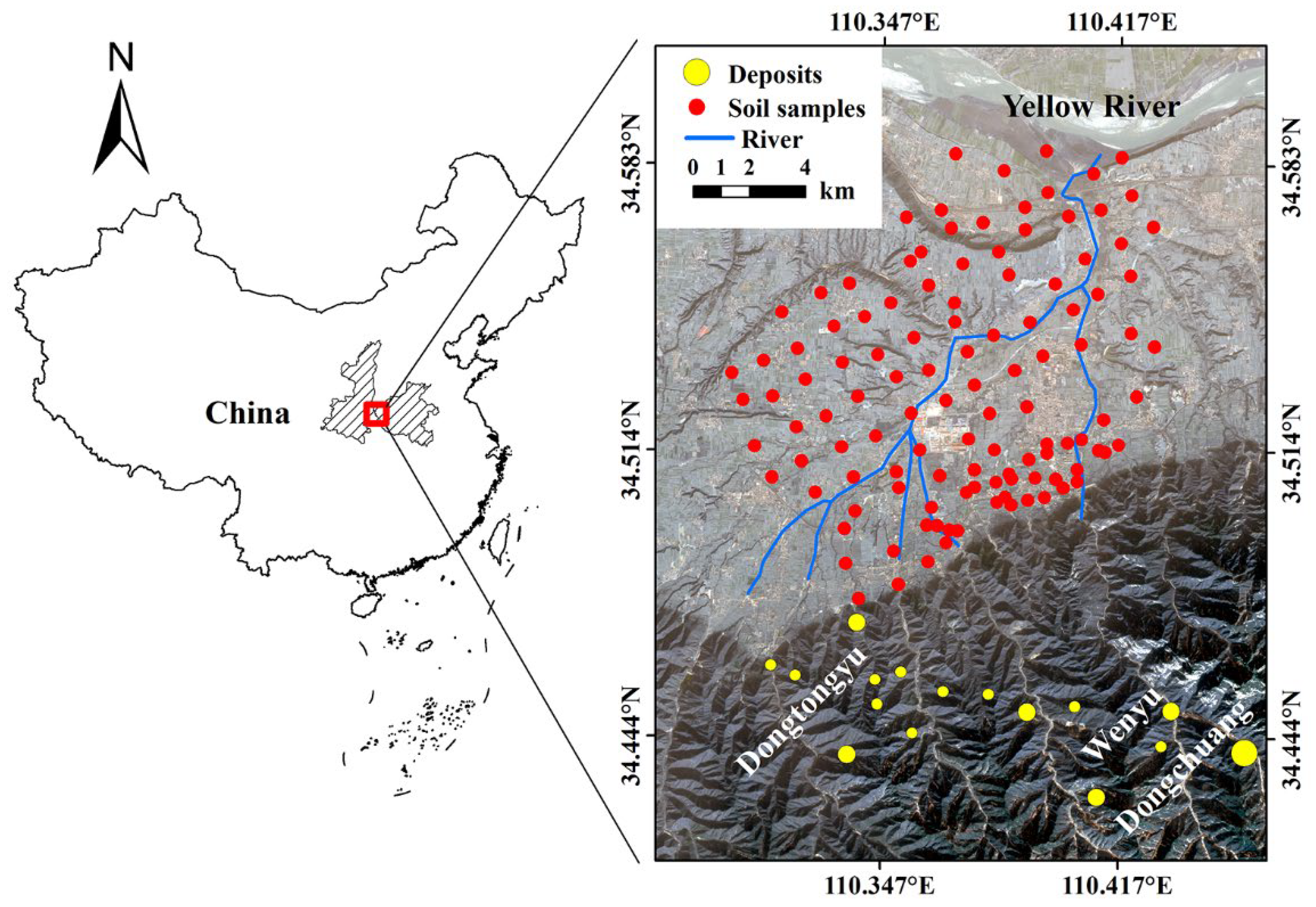
2.1. Study Area

The Xiaoqinling Mountain area is situated at the conjunction of Shaanxi and Henan Province (Figure 1), China. The sampling site (110°26′04″E to 110°37′54″E and 34°28′22″N to 34°36′19″N) is situated 10 km north from active mining and smelting facilities. The farmlands are mainly distributed on the alluvial plains downstream from a series of gold deposits. The elevation of these farmlands decreases from 653 m in the south to 323 m in the north. The soil is alkaline, and the pH of the soils is 7.5 to 8.0, with 645.8 mm annual precipitation. Rivers and valleys are well developed in the area, and all flow into the Yellow River in the north [27]. The site contains five different types of soil: warp soil, brown soil, cinnamon soil, sandy clay soil, and dark loessial soil. The soil types are controlled by either the host rock or local topography, e.g., warp soil is found predominantly in low-altitude valleys [28].
Three large gold deposits (Dongtongyu, Wenyu, and Dongchuang) and a few small-medium gold mines are located in the research area (Figure 1). In these deposits, quartz veins, altered fracture zones, and Pb mineralization frequently occur together with Au mineralization [29]. Long-term and large-scale mining activities have resulted in soil heavy metal contamination, especially Pb, Hg, Cd, etc., in the farmland around the Xiaoqinling Mountain, and Pb is considered as one of the most common contamination indicators of the study area [20,30].

2.2. Data and Preprocessing

2.2.1. Sampling and Laboratory Analysis

A total of 115 topsoil samples (1 kg per sample) were collected in the area at a depth of 0–8 cm in August 2019 (Figure 1). A regular grid was scheduled to guide field sample collection, and a portable GPS (Garmin, Lenexa, KS, USA) was used for positioning with a positioning accuracy of 5 meters. The samples covered an area of 100 km2 with an average interval of approximately 1 km. The grass, debris, and stones were physically removed from the samples after they were air-dried under natural conditions.
The Pb content of the soil samples was obtained in the laboratory by an Olympus Delta Premium portable X-ray fluorescence (pXRF, Waltham, MA, USA). The pXRF instrument was set to soil mode, and a contact detector was utilized to make measurements on sample surface. The instrument was calibrated with a metal alloy disc for every 15 samples. The detection limits of the pXRF method for Pb and Fe are 5 mg/kg and 20 mg/kg, respectively [31]. The quality control (QC) of the measurement was confirmed using standard reference samples certified by National Institute of Standards and Technology (NIST). The correlation coefficient between the measured values and the reference values was higher than 0.95. This method has been proven to be a quick and relatively accurate approach for measuring Pb content in soils [32,33]. The mineral composition of 12 representative soil samples was determined by Shimadzu X-ray diffractometer (XRD, Lab XRD-6100, Kyoto, Japan) in the laboratory. Each sample was grounded and sieved (25 μm) before being analyzed at a 20 °C temperature and 40% humidity. The 2θ scans were conducted from 5° to 80° at a 2°/min speed. Results were processed using the MDI Jade 6.0 software (Material Data, Inc., Livermore, CA, USA) with card PDF2-2004.
Based on the National Risk Control Standard for Soil Contamination of Agricultural Land (NRCSSCAL, GB 15618-2018), combined with pH values of the study area, the risk screening value (RSV), the risk control value (RCV), and the soil background value (SBV) of Pb are 170 mg/kg, 1000 mg/kg, and 16.3 mg/kg, respectively. Quick statistics (Table 1) of the sample pXRF data indicate that many samples’ Pb content was much higher than the SBV in this area out of 115 samples, 60 (more than 52%) exceeded the RSV threshold and were thus considered Pb contaminated. Moreover, the coefficient of variation (CV), defined as the ratio of the standard deviation (SD) to the mean value of heavy metal content in soil, shows the great difference in Pb content due to the large CV value (1.67). In addition, Pb data were transformed to the log scale for further spectral analysis, as is common practice for predicting the contamination of soil heavy metals [34,35]. The log-transformed Pb (ln(Pb)) data are close to a normal distribution with the skewness and kurtosis values close to 0, which is more suitable for further statistical analysis and modelling than the original Pb values. Due to the nature of the link between the absorption coefficient and the intimate combination of soil compositions, it is easier to characterize soil element contents in the log scale using reflectance spectra [36,37].

2.2.2. Data for Soil Properties

The soil pH, soil organic carbon (SOC) and CEC were collected to analyze the association between Pb concentration and soil properties in the study. The soil pH, SOC and CEC data (at spatial interval of 90 meters) were obtained from the National Earth System Science Data Center, National Science & Technology Infrastructure of China (http://www.geodata.cn (accessed on 13 April 2022)) [38,39], and the average values of the topsoil (0–5 cm) pH, SOC and CEC from 2010 to 2018 were used to analyze the potential influence factors of Pb concentration in this research.

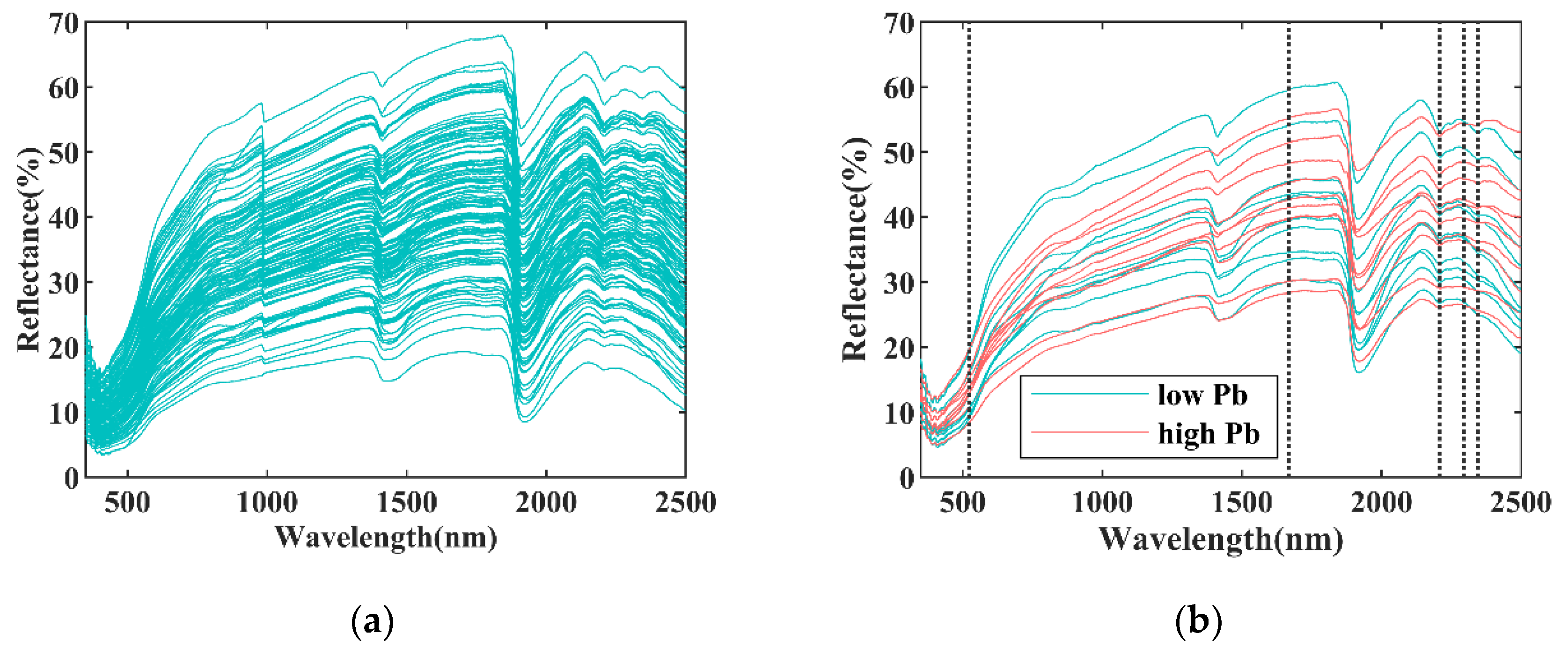
2.2.3. Spectral Measurement and Preprocessing

The spectral data were collected by SR-3500 spectrometer (Spectral Evolution Inc., Lawrence, MA, USA) in a laboratory, between 350 nm and 2500 nm in spectral range. The spectral resolution was 3 nm (350–1000 nm), 8 nm (1000–1900 nm), and 6 nm (1900–2500 nm), with a 1 nm sampling bandwidth. Bare fiber with a contact probe was used to measure radiance from these soil samples illuminated by a halogen lamp (5W, 7.4V) with a 25° incidence angle. The radiance spectrum was normalized to that of a 99% Spectralon white panel to obtain a reflectance spectrum. Ten spots were measured for each sample, with a field of view of 2 cm in diameter and average of 25 co-adds for each spot, and the representative spectrum for each sample was then obtained by averaging the ten spectra. The artificial steps/breakpoints at 980 nm caused by adjacent sensors were corrected (Figure 2).

2.3. Spectral Bands Extraction and Modelling

Continuum removal (CR) is a popular spectral analysis technique for removing the spectral background and enhancing absorption features [40,41,42]. The continuum is a convex hull fitted between the starting and ending points of the absorption features. The first and last band values of the CR–processed spectrum are equal to 1 because the raw bands are on the hull, whereas the other bands have values between 0 and 1 [40,41]. The CR method can be described as follows [43]:
C i = R i / R c i
where C i is the value of the continuum-removed reflectance spectrum at the band i; R i is the value of the original reflectance spectrum for band i; R c i is the value of the continuum at the band i. The starting bands and ending bands are set as 350 nm and 2500 nm in this research.
After continuum removal of a spectrum, the strength of absorption features can be attributed to the physical properties of the measured target. The Pearson correlation coefficient (r) was applied to measure the relationship between the continuum removed soil spectra and Pb content to extract the sensitive bands for further modelling in this study [44].
A set of rules was used to assess the band sensitivity to Pb content. Firstly, the absorption features that have mineralogical meaning were identified on a continuum removed spectra. Each feature was defined by a spectral range (see Section 3.1 for feature ranges). Then, the Pearson correlation coefficient between each band of the continuum removed the reflectance and Pb content was calculated. All bands with a correlation coefficient larger than 0.1 and with band positions falling within the feature ranges identified in previous step were retained. All spectral bands with correlation coefficients larger than 0.4 were retained, regardless of whether these bands show absorption features or not. All these retained bands are candidates for being subjected to further processing. Secondly, the band with the highest correlation within each feature range was selected and set as reference band for this feature. The correlation coefficients between this reference band and all other retained bands in this range were calculated and compared. One or more bands were added to the sensitive band set if the correlation coefficients between the reference band and all the other bands were less than 0.9 in order to remove band collinearity within each absorption feature. This process was conducted in each feature range, and finally, 31 sensitive bands were retained for further modelling. Thirdly, the PLSR was used to build prediction models using the 31 sensitive bands. Progressive iteration/optimization was conducted by removing one band with the lowest regression coefficient value (see Section 3.3 for detail). The number of bands in the model was reduced through the iterative process to improve adaptability in future applications.

2.4. PLSR Modelling and Validation

PLSR is commonly used for quantitative spectral analysis [45,46] when the sample size is small [9]. This study used the PLSR method to model the relationship between Pb content (dependent variable) and the continuum removed reflectance at sensitive bands (independent variables). Three-quarters of the total sample suite (88 out of the 115 samples) were used for modelling, and a quarter (27 out of the 115 samples) was retained for independent model validation. A large number of independent variables (spectral bands) with a small number of dependent variables (Pb content) leads to a high possibility for overfitting [47,48]. Only 31 sensitive bands were involved as initial independent variables (as described in Section 3.1), reducing the risk of overfitting. The standardized regression coefficients of the PLSR method indicate the importance of each predictor in the model and correspond to the standardized variables [49,50,51]. The standardized regression coefficients were used to further optimize the initial PLSR model by removing one band with the lowest regression coefficient value iteratively to optimize the number of spectral features. Considering the fact that the accuracy of the PLSR model was stable when the number of sensitive bands was more than 5 and the number of samples is 88 (see Section 3.3 for detail), and these 5 bands were located at separate spectral regions with different physical meaning, the risk of overfitting is extremely low.
R2, residual prediction deviation (RPD), and root mean square error (RMSE) were used to assess the PLSR model’s accuracy. The efficiency of the prediction model was evaluated by comparing the correlation between the predicted and measured Pb concentrations. The evaluation system of Rossel et al. [52] was adopted: RPD ≤ 1.0 indicates unsuccessful predictions, 0 < RPD ≤ 1.4 indicates poor predictions, 1.4 ≤ RPD < 1.8 indicates fair predictions, 1.8 < RPD ≤ 2.0 indicates good predictions, 2.0 < RPD ≤ 2.5 indicates very good quantitative predictions, and RPD > 2.5 indicates excellent predictions. Generally, a good model has large values of R2 and RPD with low RMSE [53]. The formulas for the three parameters are as follows:
R 2 = 1 n i = 1 n ( y ^ i y i ) 2 / 1 n i = 1 n ( y i y ¯ ) 2
RMSE = 1 n i = 1 n ( y ^ i y i ) 2
RPD = 1 n i = 1 n ( y i 1 n i = 1 n y i ) 2 / 1 n i = 1 n ( y ^ i y i ) 2
where y i is the measured Pb content of the i th sample; y ^ i is the predicted Pb content of the i th sample; y ¯ is the average of the measured Pb content of the samples; n is the number of samples.

2.5. Ordinary Kriging

After the Pb value of each sample location was predicted, the ordinary kriging (OK) interpolation method [54] was employed to map the spatial distribution of soil Pb contamination. The weights of OK are averages of the observations based on the degree of spatial correlation [55], and OK is commonly considered as an unbiased estimator [56,57] for the observations following spatial grids with regular intervals, which is appropriate to this research.

3. Results

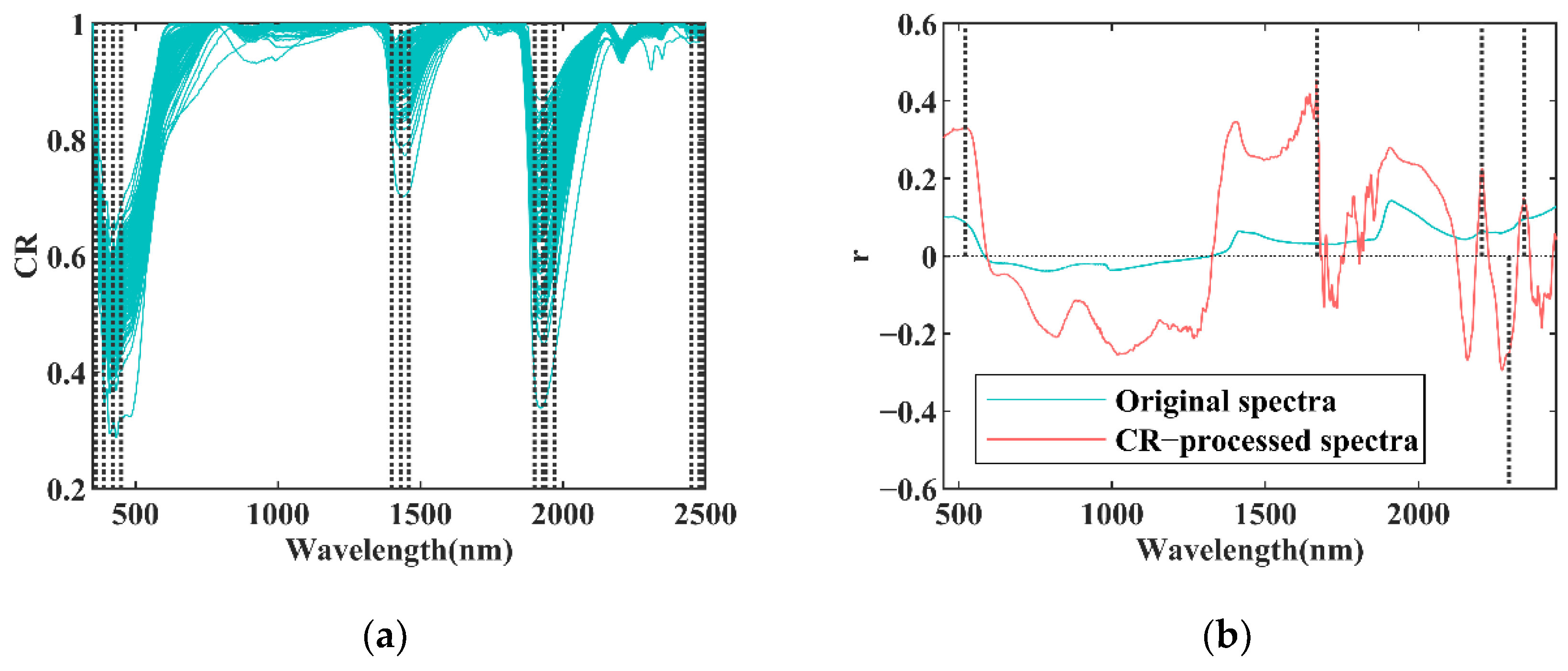
3.1. Sensitive Bands

Spectral data at wavelengths lower than 450 nm and longer than 2450 nm were eliminated (Figure 3a), and bands near water features (1400 nm and 1900 nm) were not included in band selection. The continuum removed spectra clearly show a series of spectral features at 450–600 nm, 710–735 nm, 780–790 nm, 820–950 nm, 1010–1024 nm, 1120–1132 nm, 1350–1368 nm, 1560–1580 nm, 1745–1820 nm, 1850–1875 nm, 2150–2235 nm, 2240–2265 nm, 2280–2305 nm, and 2310–2360 nm (Table 2). Compared to the original spectrum, the correlation between the continuum removed soil spectrum, and Pb content has significantly increased (Figure 3b). The maximum single band correlation coefficient between the original spectra and Pb content is about 0.15. In contrast, the maximum correlation coefficient between continuum removed spectra, and Pb content increased to about 0.45 (Figure 3b). The bands with higher correlation are mainly distributed around 450–575 nm, 716–1316 nm, 1343–1677 nm, 1710–1714 nm, 1721–1736 nm, 1826–2103 nm, 2137–2181 nm, 2197–2220 nm, 2250–2317 nm, 2332–2356 nm, 2317–2387 nm, and 2394–2410 nm for both of the original spectra and the CR–processed spectra (Figure 3b). All the individual sensitive bands are listed in Table 2. As the absorption strength of adjacent bands is often correlated, 31 sensitive bands were finally selected to reduce redundancy based on the method described in Section 2.3 (Table 2).

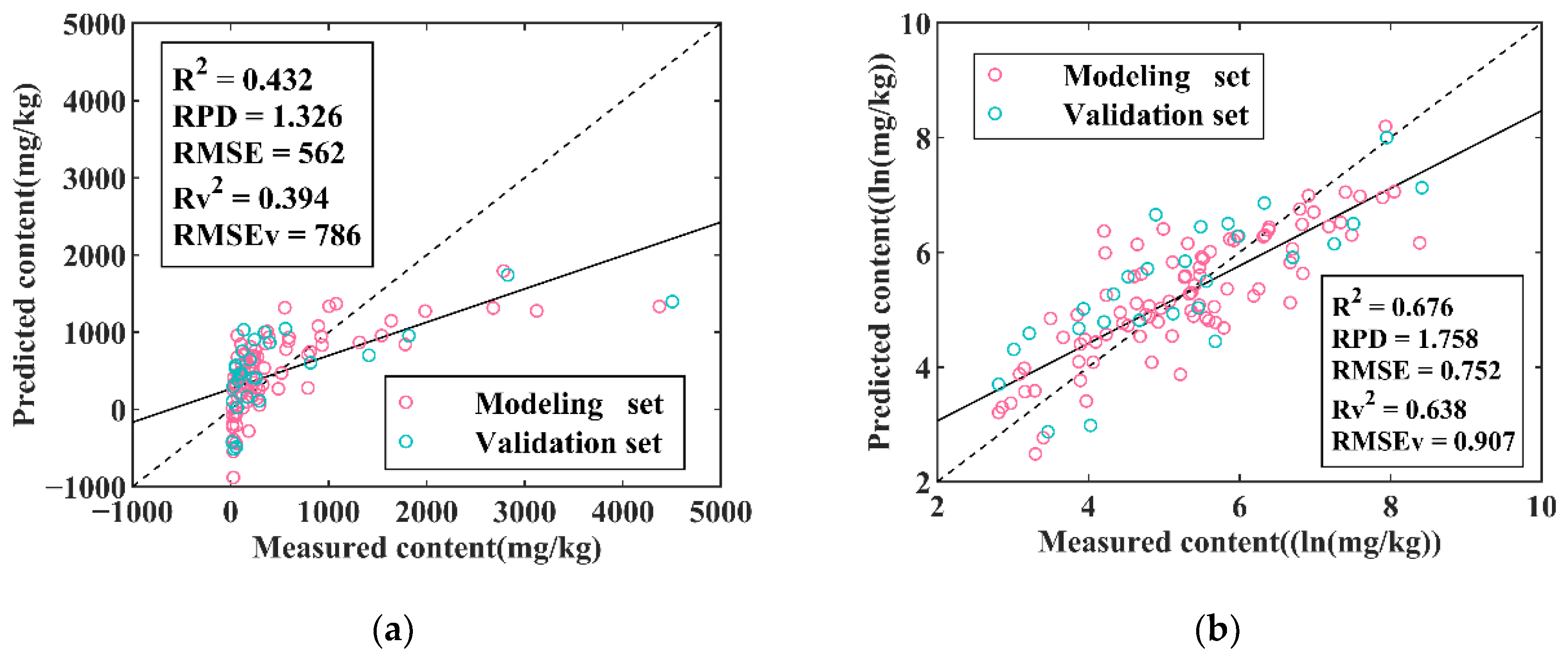
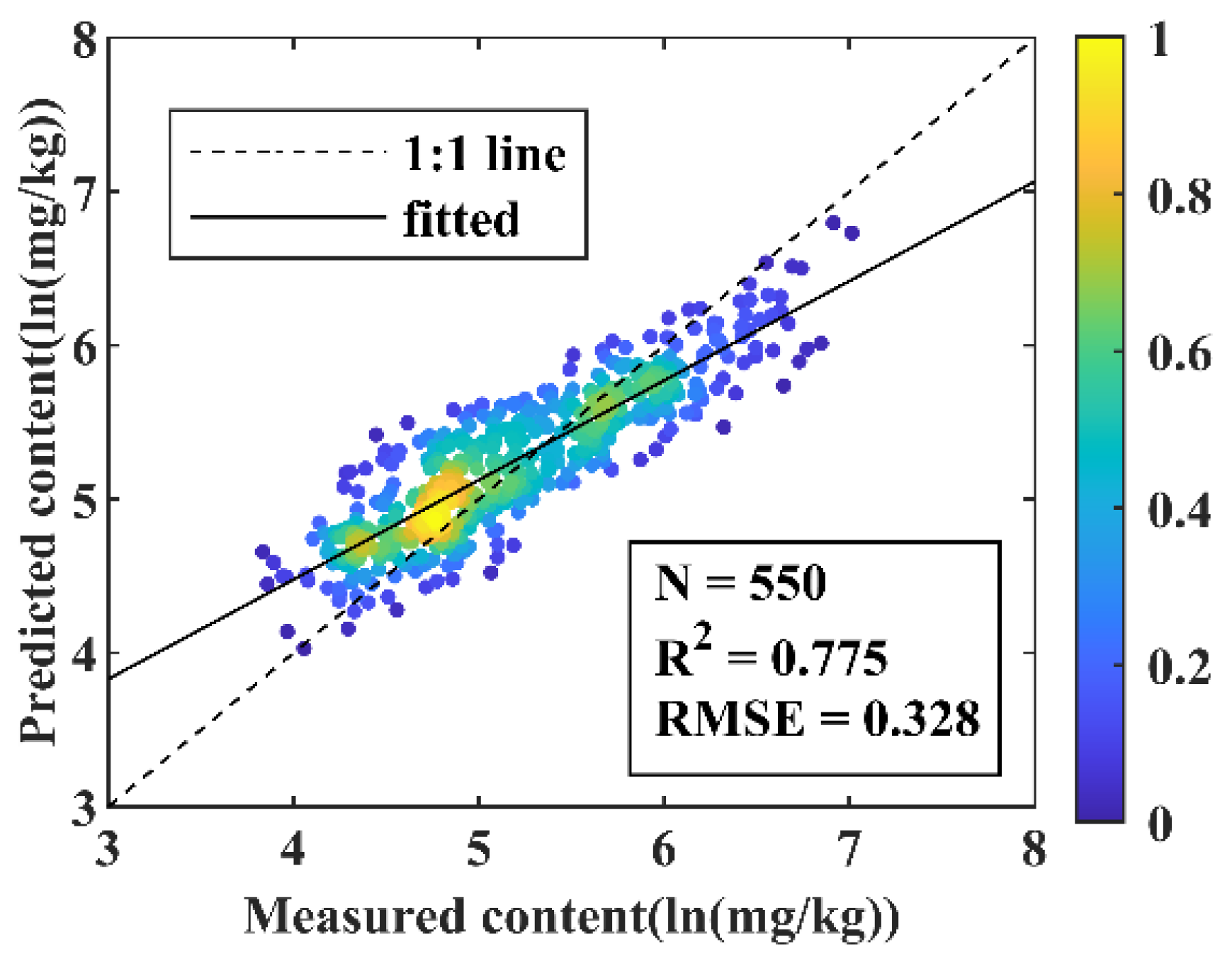
3.2. Model Construction and Validation

The 115 topsoil samples were ranked in the order of Pb content from lowest to highest. One sample was retained for validation from every four samples sequentially. Thus, the 115 soil samples were separated into 88 for modelling and 27 for validation. The statistics of the modelling and validation suite are shown in Table 3. Both the original Pb content and the log-transformed Pb content were tested for modelling, with all the 31 sensitive bands shown in Table 2.
The R2, RPD, and RMSE of modelling with the original Pb content were 0.432, 1.326, and 562 mg/kg, respectively. R2 and RMSE of validation suite ( R v 2 and RMSEv) were 0.394 and 786 mg/kg, respectively (Figure 4a). The poor R2 implies that the model cannot estimate the Pb concentration of the soil quantitatively, especially for low Pb samples. After log-transformation of Pb, the R2, RPD and RMSE for modeling were 0.676, 1.758 and 0.752 ln(mg/kg), respectively, and the R v 2 and RMSEv of validation samples were 0.638 and 0.907 ln(mg/kg) (Figure 4b). The results indicated that modelling with log-transformed Pb significantly improved the model performance. As a result, only log-transformed Pb (ln(Pb)) was used in all subsequent process.

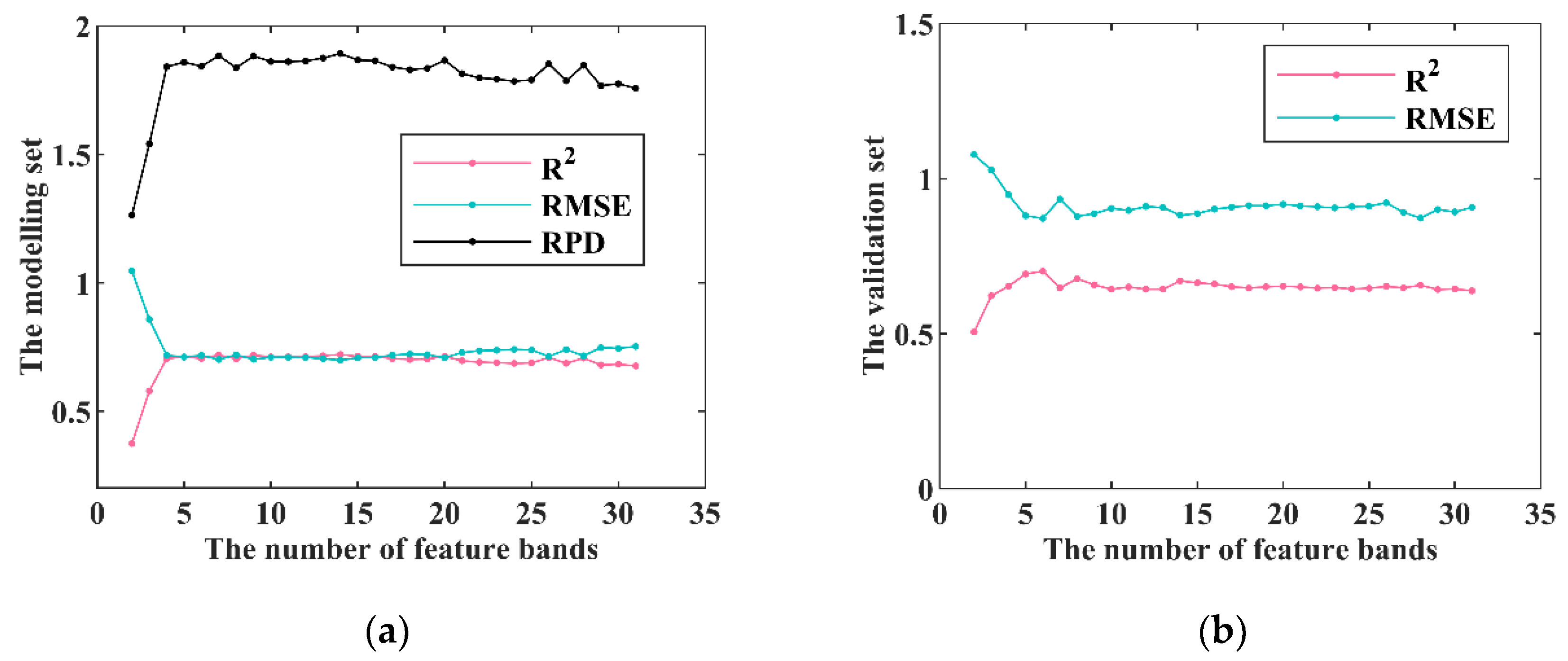
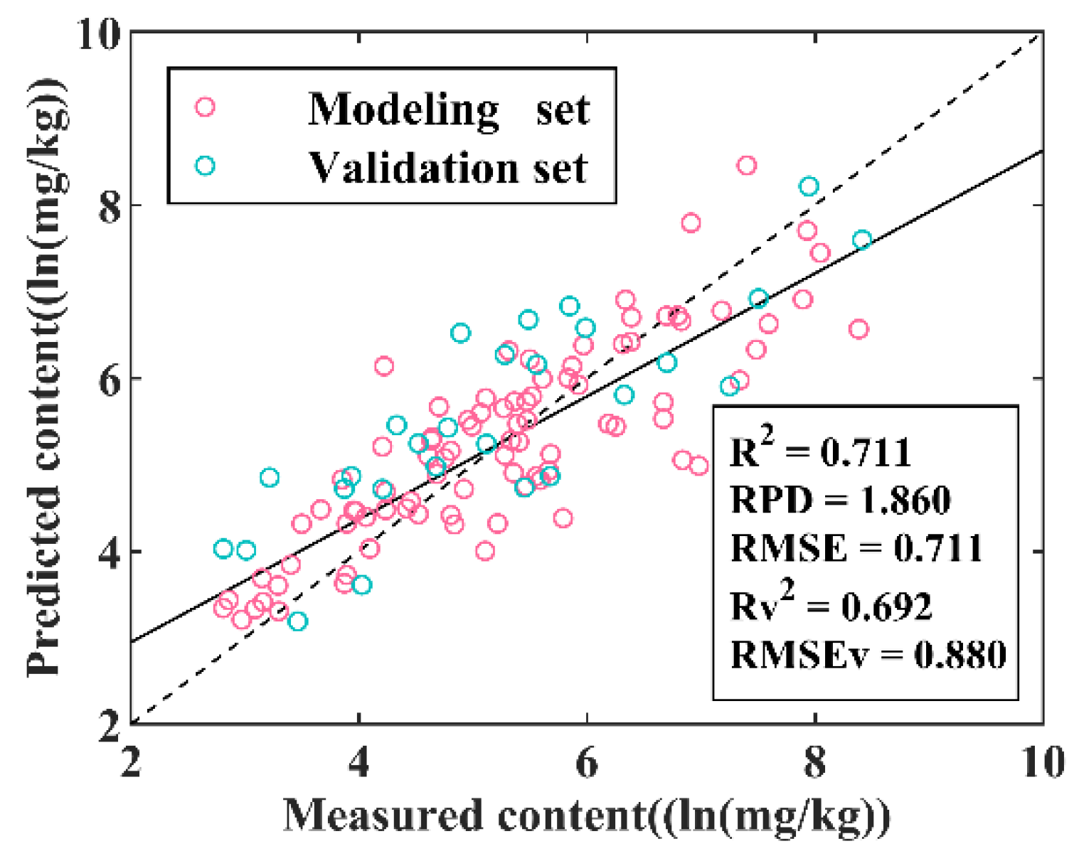
3.3. Optimization of Model

The adjacent spectral bands of hyperspectral data are strongly correlated with high data redundancy [58]. Some sensitive bands are very close to each other within the same feature range. Therefore, in order to reduce the dimensionality of spectra and the collinearity of bands, an iterative process was conducted to reduce the number of the bands, one band with the lowest standardized regression coefficient value in the regression model was removed in each iteration. Figure 5 illustrates the accuracy variation for modelling and validation samples with 2–31 sensitive bands. For PLSR model with 5–7 sensitive bands, the standardized regression coefficient is stable. In addition, the 5–band model was used to generate final results as these five bands fell into different feature ranges with different physical meaning.
When the number of feature bands was higher than 5, the R2 and RMSE of the modelling and validation samples, as well as the RPD of the modelling set, remained stable (Figure 5a,b). The accuracy decreased dramatically when the number of bands was less than 5 for both validation and modelling samples. Thus, the optimized model (Equation (5)) used 5 features/bands: 522 nm, 1668 nm, 2207 nm, 2296 nm, and 2345 nm (Figure 2b, Figure 3b and Figure 6). The bands captured the significant spectral variations observed in CR–processed reflectance (see Section 3.1). The R2, RMSE, and RPD of the optimized model (Figure 6) are comparable to the results of the model using all 31 bands (Figure 4b).
Y = 728.1 + B 522 9.8 + B 1668 640.9 + B 2207 34.2 + B 2296 116.8 + B 2345 173.5
where Y is the log-transformed Pb content with the unit ln(mg/kg).

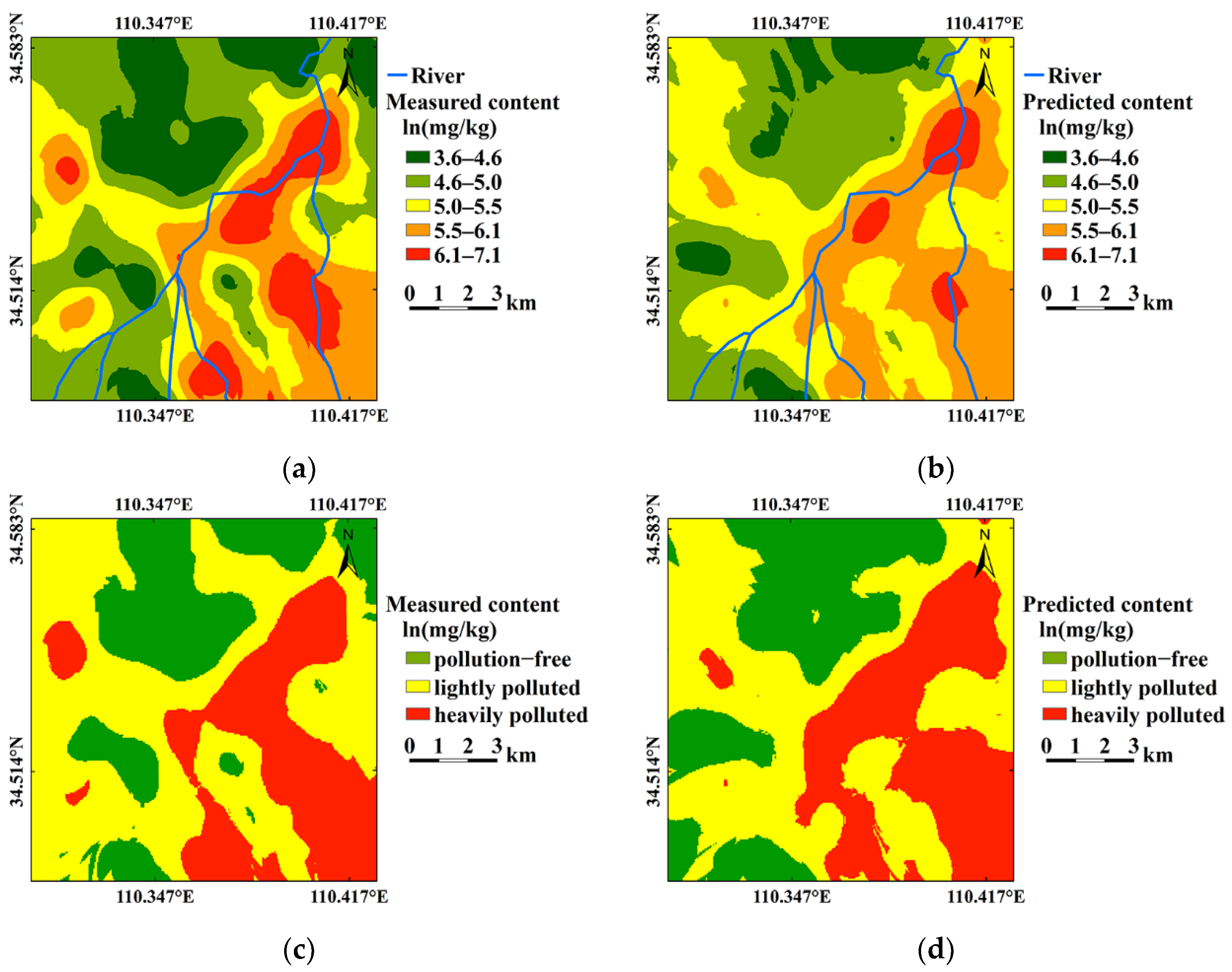
3.4. Spatial Distribution of Soil Pb Contamination

Figure 7 compares the distribution maps obtained via OK interpolation from the measured Pb (Figure 7a) and model predicted Pb (Figure 7b). The model highlights all of the notable Pb anomalies in the area. Based on the NRCSSCAL, two thresholds, the logarithm of RSV (ln(RSV) = 5.14 ln(mg/kg)), and the logarithm of RCV (ln(RCV) = 6.91 ln(mg/kg)) of the Pb were used to evaluate the contamination, which was divided into 3 levels. Values less than 5.14 ln(mg/kg) were considered as pollution–free areas, values between 5.14 ln(mg/kg) and 6.91 ln(mg/kg) were lightly polluted areas, and values greater than 6.91 ln(mg/kg) were defined as heavily polluted areas (Figure 7c,d). The two Pb contamination maps interpolated from the measured values and predicted values were compared visually (Figure 7c,d) and the results showed similar spatial patterns for the three contamination levels. The heavily polluted areas are spatially associated with the drainages. The maps indicate that the source material of Pb contamination was transported from upstream by flood and affected by the deposits and mining activity. Therefore, the Pb content may be negatively correlated to elevation and result in the differences of the soil type and minerals in soil. The visual comparison of these maps also indicates that most areas with heavy soil Pb pollution can be identified on prediction map (Figure 7b,d). Both Figure 7a (measured map) and Figure 7b (predicted map) were resampled to 0.005 degrees per pixel for map comparison (total of 550 pixels in the area). Figure 8 shows that the two maps are highly comparable with high R2 (0.775) and low RMSE (0.328 ln(mg/kg)). However, the maximum value of predicted data was slightly lower than the observed data (Figure 8).

4. Discussion

4.1. Selection of Sensitive Bands

Hyperspectral spectra with continuous spectral bands and narrow bandwidth enable accurate determination of target properties, but the strong correlation between adjacent spectral bands poses high data redundancy [58]. Band selection can reduce the dimensionality of spectra to facilitate the separation of different targets [59]. In this study, 31 sensitive bands were selected by correlation analysis between spectrum and Pb content, spectral absorption features, and the correlation among the bands within spectral ranges of each feature (Table 2). The iterative process further reduced the number of the bands to 5 by monitoring the standardized regression coefficient value in each iteration with different band combinations. The five bands—522 nm, 1668 nm, 2207 nm, 2296 nm, and 2345 nm—were located within different spectral regions/features, and thus considered independent variables in the final prediction model (Figure 2b and Figure 3b). However, there are different approaches for best variable/band selection during the iteration, e.g., backward and forward selection. Prior knowledge must be used to make the final decision. In this study, the model’s performance (Figure 5) hit a tipping point at band numbers 5–7, where the statistical performance of the model starts to stabilize. However, combining diverse absorption qualities with physical meaning increases the model’s adaptability.

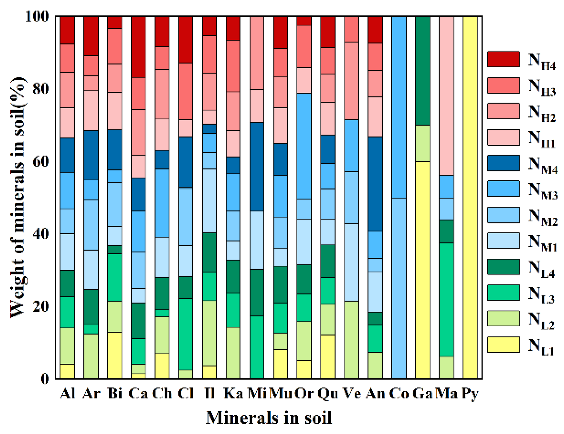
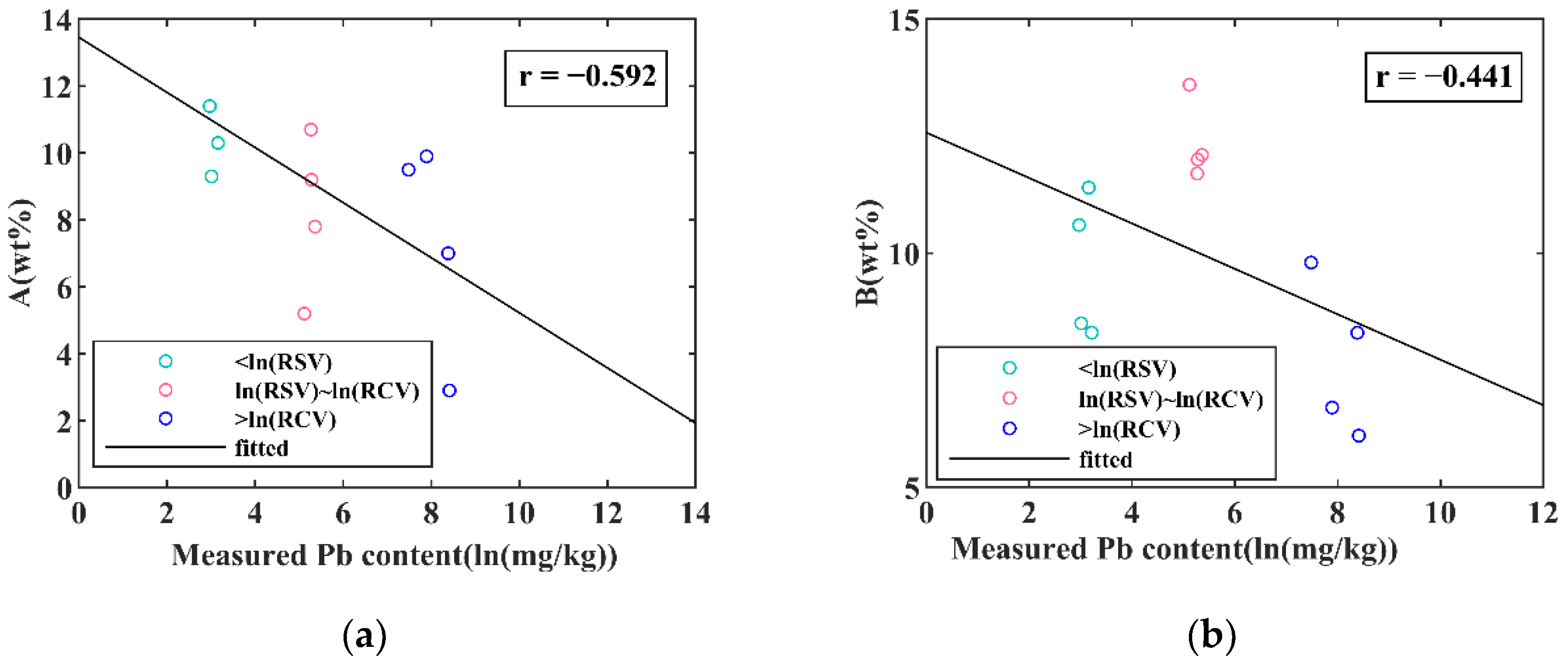
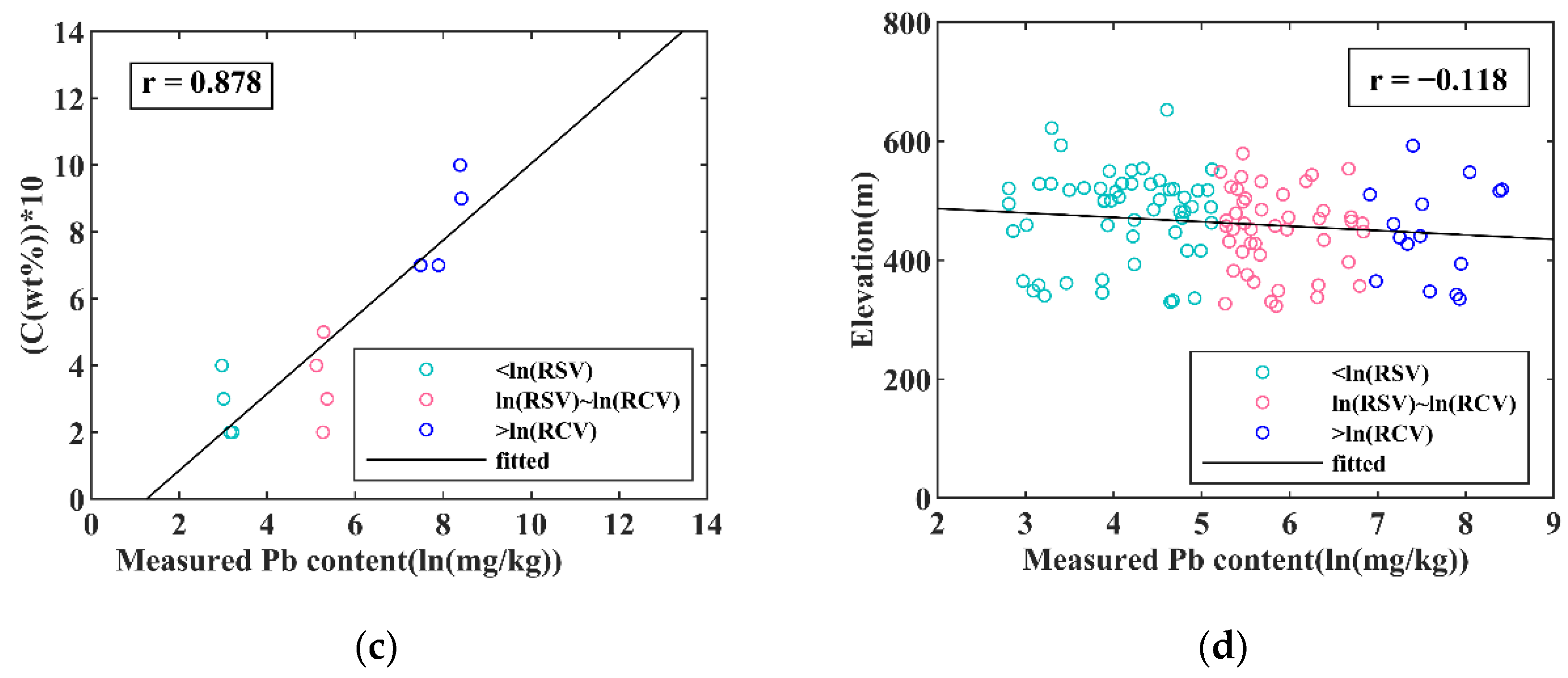
4.2. Mineralogy of Samples

Figure 9 presents the XRD data from the 12 representative samples (4 samples with Pb lower than RSV, 4 samples with Pb higher than RCV, and 4 samples with Pb between RSV and RCV) to understand the physical mechanism of the prediction model. Clinochlore, biotite, albite, calcite, quartz, illite, kaolinite, and muscovite were detected from all the selected soil samples, with varying contents. It is observed that the Pb content is negatively correlated with the summation of calcite, chlorite, and clinochlore, all of which show absorption features near 2340 nm (Figure 10a). Similarly, the Pb content is negatively correlated with the summation of kaolinite, illite, and muscovite, showing absorption features near 2200 nm (Figure 10b). Furthermore, XRD data showed that high Pb samples contain more Pb-bearing minerals. Anglesite (Pb(SO4)), cotunnite (PbCl2), galena (PbS), massicot (PbO), and pyromorphite (Pb5(PO4)3Cl) are all detected (Figure 9 and Figure 10c).
Previous research indicated that the 500–600 nm region is full of charge transfer absorptions of Fe3+, Cr3+, Mn2+, etc. [26,60]. The range of 1600–2400 nm in a spectrum is dominated by the absorption features of electronic and vibrational processes from bonds and hydroxyl [60]. The spectral absorption of hydroxyls in clay minerals (such as illite and kaolinite) and muscovite are close to 2197–2210 nm [10,61]. The absorption feature of phyllosilicate minerals (such as chlorite) is around 2320–2350 nm [61]. Several studies have demonstrated that the carbonate minerals (mainly calcite) at the surface of soil have a significant adsorption capacity for Pb [23,62,63], and the absorption feature of carbonate minerals is in the range of 2310–2335 nm [10,60]. As a result of the negative correlation between Pb and the summation of calcite, chlorite, and clinochlore (Figure 10a), as well as the negative correlation between Pb and the summation of kaolinite, illite, and muscovite (Figure 10b), samples with high Pb content should have weak absorption characteristics at 2207 nm and 2345 nm. In contrast, samples with low Pb content should have strong absorption characteristics at 2207 nm and 2345 nm.

4.3. Impact of Topography and other Factors

Figure 7a suggests that the spatial distribution of high Pb generally follows the topographical valley. Figure 10d confirms that the logarithm of Pb is negatively correlated to elevation, even though the correlation is very low (r = −0.118) and the deviation is high. It was observed that locations with high Pb content generally fall within the distribution of warp soil [28]. The warp soil was formed by fluvial outwash. It is likely that the source material was transported from upstream and affected by mining activity. This can also be explained by the fact that Pb-bearing minerals of the high Pb samples are dominated by galena (PbS) and massicot (PbO) (Figure 9).
The samples with low Pb are mostly from sandy clay soil and dark loessial soil with a relatively high content of clay minerals and carbonates, while anglesite (Pb(SO4)) is the dominant Pb-bearing mineral (Figure 9). This is confirmed by previous investigation [64] that in ordinary mature soil Pb exists most likely in the form of PbSO4 and PbCO3 with a higher bioaccessibility than galena.
The distribution of Pb in soil is affected by many factors, e.g., soil Fe, pH, CEC and SOC [22,23,65]. In this study, the soil pH is negatively correlated with Pb content with correlation coefficient −0.392 (Table 4). The Fe, CEC, and SOC are positively correlated with Pb content, and the correlation coefficients are 0.446, 0.190, and 0.394, respectively. Therefore, the samples with high Pb content tend to be distributed at areas with low pH, high Fe, SOC, and CEC (Figure 11), which is probably due to the decrease of pH that is conducive to the accumulation of soil Pb [66]. The SOC and Fe were highly and positively correlated with Pb, which is consistent with previous research [67,68] and results in the absorption features in the VNIR-SWIR range.

4.4. Accuracy and Adaptability of the Prediction Model

The accuracy of prediction can be affected by many factors such as sampling strategy, sample preparation, feature selection, instrumental instability, etc. In this investigation, samples were collected using a standard sampling grid approach. Multi-spot spectral average in data collection increased the signal-to-noise ratio and made the spectrum representative of each sample. To determine the accuracy of Pb content by pXRF, 21 samples were analyzed for Pb content using inductively coupled plasma-atomic emission spectroscopy (ICP-AES) on the Thermo-Fisher iCAP 6300 apparatus in the laboratory. The results showed that the Pb content measured by pXRF was comparable to the values analyzed in the laboratory, with a correlation coefficient 0.97. The final prediction model was built on a minimal number of independent features/bands to increase its adaptability for new applications in similar terrains and soil types. With fewer bands in the prediction model, it is much easier to adapt the methodology to similar terrains with much simpler spectrometer, or device new instruments for quick or real-time in situ Pb prediction. Additionally, the five spectral features/bands in the model are all located within the atmospheric window. This provides an opportunity to test this Pb prediction model with satellite imaging data, which has large spatial coverage and is more cost-effective.

5. Conclusions

This study used PLSR to establish the relationship between soil Pb content and continuum removed reflectance spectra in the visible to shortwave infrared region. The result showed that bands at 522 nm, 1668 nm, 2207 nm, 2296 nm, and 2345 nm are correlated to the log-transformed Pb content (ln(mg/kg)). The PLSR model achieved an accuracy of R2 = 0.711 and validated at R2 = 0.692 from 27 independent validation samples.
The predicted map of Pb values follows the same spatial pattern as the map of measured Pb data using the OK interpolation method. This suggests that Pb contamination levels of farmland soil can be quickly predicted from VNIR-SWIR spectra, especially the high Pb anomalies.
This study also demonstrates the need to optimize the model by employing the minimal number of physical bands possible. More bands in the prediction model do not necessarily increase the accuracy due to spectral collinearity. The XRD data prove that Pb content is negatively linked with the sum of calcite, chlorite, and clinochlore. The total of kaolinite, illite, and muscovite is also negatively linked with Pb concentration. Furthermore, XRD measurements reveal that samples containing a high concentration of Pb have a greater proportion of Pb-bearing minerals. Anglesite (Pb(SO4)), cotunnite (PbCl2), galena (PbS), massicot (PbO), and pyromorphite (Pb5(PO4)3Cl) were all detected. In addition, the Pb anomalies are primarily located in warp soil formed by fluvial outwash, suggesting Pb contamination is from upstream mining activities.
The five spectral features/bands in the model are all located within the atmospheric window, although the spectra used in this study were acquired in the laboratory. This opens the opportunity of testing the prediction model to detect Pb anomalies using satellite imaging data, which will provide an even cost-effective option to quickly map the distribution of soil Pb content over broad areas in much finer details (meter scale).

Author Contributions

Conceptualization, L.L.; Formal analysis, L.L. and J.F.; Funding acquisition, L.L.; Investigation, D.X., F.Y. and L.L.; Methodology, D.Z. and L.L.; Project administration, F.Y. and L.L.; Resources, F.Y.; Writing—original draft, D.Z.; Writing—review & editing, L.L., J.F. and T.A.; D.Z. and L.L. have equal contributions. All authors have read and agreed to the published version of the manuscript.

Funding

This research was funded by the National Natural Science Foundation of China (42071258), Fund Project of Shaanxi Key Laboratory of Land Consolidation (2018-ZY04), Natural Science Foundation of Shaanxi (2022JQ-240), and Special Fund for Basic Scientific Research of Central Colleges (No. 300102352102), Chang’an University, China.

Data Availability Statement

Not applicable.

Acknowledgments

Acknowledgement for the data provide by National Earth System Science Data Center, National Science & Technology Infrastructure of China (http://www.geodata.cn (accessed on 13 April 2022)).

Conflicts of Interest

The authors declare no conflict of interest.

References

  1. Fei, X.; Lou, Z.; Xiao, R.; Ren, Z.; Lv, X. Contamination assessment and source apportionment of heavy metals in agricultural soil through the synthesis of PMF and GeogDetector models. Sci. Total Environ. 2020, 747, 141293. [Google Scholar] [CrossRef] [PubMed]
  2. Luo, X.; Ren, B.; Hursthouse, A.S.; Thacker, J.R.M.; Wang, Z. Soil from an Abandoned Manganese Mining Area (Hunan, China): Significance of Health Risk from Potentially Toxic Element Pollution and Its Spatial Context. Int. J. Environ. Res. Public Health 2020, 17, 6554. [Google Scholar] [CrossRef] [PubMed]
  3. Fashola, M.O.; Ngole-Jeme, V.M.; Babalola, O.O.; Naeth, M.A. Physicochemical properties, heavy metals, and metal-tolerant bacteria profiles of abandoned gold mine tailings in Krugersdorp, South Africa. Can. J. Soil Sci. 2020, 100, 217–233. [Google Scholar] [CrossRef]
  4. Kabala, C.; Singh, B.R. Fractionation and Mobility of Copper, Lead, and Zinc in Soil Profiles in the Vicinity of a Copper Smelter. J. Environ. Qual. 2001, 30, 485–492. [Google Scholar] [CrossRef] [PubMed] [Green Version]
  5. Liu, G.; Tao, L.; Liu, X.; Hou, J.; Wang, A.; Li, R. Heavy metal speciation and pollution of agricultural soils along Jishui River in non-ferrous metal mine area in Jiangxi Province, China. J. Geochem. Explor. 2013, 132, 156–163. [Google Scholar] [CrossRef]
  6. Sawut, R.; Kasim, N.; Abliz, A.; Hu, L.; Yalkun, A.; Maihemuti, B.; Qingdong, S. Possibility of optimized indices for the assessment of heavy metal contents in soil around an open pit coal mine area. Int. J. Appl. Earth Obs. Geoinf. 2018, 73, 14–25. [Google Scholar] [CrossRef]
  7. Wang, Z.; Luo, Y.; Zheng, C.; An, C.; Mi, Z. Spatial distribution, source identification, and risk assessment of heavy metals in the soils from a mining region: A case study of Bayan Obo in northwestern China. Hum. Ecol. Risk Assess. Int. J. 2020, 27, 1276–1295. [Google Scholar] [CrossRef]
  8. Kemper, T.; Sommer, S. Estimate of heavy metal contamination in soils after a mining accident using reflectance spectroscopy. Environ. Sci. Technol. 2002, 36, 2742. [Google Scholar] [CrossRef]
  9. Zhang, Z.; Ding, J.; Zhu, C.; Wang, J. Combination of efficient signal pre-processing and optimal band combination algorithm to predict soil organic matter through visible and near-infrared spectra. Spectrochim. Acta A Mol. Biomol. Spectrosc. 2020, 240, 118553. [Google Scholar] [CrossRef]
  10. Leone, A.P.; Sommer, S. Multivariate Analysis of Laboratory Spectra for the Assessment of Soil Development and Soil Degradation in the Southern Apennines (Italy). Remote Sens. Environ. 2000, 72, 346–359. [Google Scholar] [CrossRef]
  11. Ben-Dor, E.; Chabrillat, S.; Demattê, J.A.M.; Taylor, G.R.; Hill, J.; Whiting, M.L.; Sommer, S. Using Imaging Spectroscopy to study soil properties. Remote Sens. Environ. 2009, 113, S38–S55. [Google Scholar] [CrossRef]
  12. Kim, H.; Yu, J.; Wang, L.; Jeong, Y.; Kim, J. Variations in Spectral Signals of Heavy Metal Contamination in Mine Soils Controlled by Mineral Assemblages. Remote Sens. 2020, 12, 3273. [Google Scholar] [CrossRef]
  13. Yin, F.; Wu, M.M.; Liu, L.; Zhu, Y.Q.; Feng, J.L.; Yin, D.W.; Yin, C.J.; Yin, C.T. Predicting the abundance of copper in soil using reflectance spectroscopy and GF5 hyperspectral imagery. Int. J. Appl. Earth Obs. Geoinf. 2021, 102, 9. [Google Scholar] [CrossRef]
  14. Pandit, C.M.; Filippelli, G.M.; Li, L. Estimation of heavy-metal contamination in soil using reflectance spectroscopy and partial least-squares regression. Int. J. Remote Sens. 2010, 31, 4111–4123. [Google Scholar] [CrossRef]
  15. Liu, J.; Zhang, Y.; Wang, H.; Du, Y. Study on the prediction of soil heavy metal elements content based on visible near-infrared spectroscopy. Spectrochim. Acta A Mol. Biomol. Spectrosc. 2018, 199, 43–49. [Google Scholar] [CrossRef]
  16. Hong, Y.; Shen, R.; Cheng, H.; Chen, Y.; Zhang, Y.; Liu, Y.; Zhou, M.; Yu, L.; Liu, Y.; Liu, Y. Estimating lead and zinc concentrations in peri-urban agricultural soils through reflectance spectroscopy: Effects of fractional-order derivative and random forest. Sci. Total Environ. 2019, 651, 1969–1982. [Google Scholar] [CrossRef]
  17. Xu, B.; Li, D.; Shi, X. A Preliminary Stndy on Identification of Clay Minerals in Soils with Reference to Reflectance Spectra. Pedosphere 1995, 5, 135–142. [Google Scholar]
  18. Komy, Z.R.; Shaker, A.M.; Heggy, S.E.; El-Sayed, M.E. Kinetic study for copper adsorption onto soil minerals in the absence and presence of humic acid. Chemosphere 2014, 99, 117–124. [Google Scholar] [CrossRef]
  19. Sun, W.; Zhang, X. Estimating soil zinc concentrations using reflectance spectroscopy. Int. J. Appl. Earth Obs. Geoinf. 2017, 58, 126–133. [Google Scholar] [CrossRef]
  20. Zhang, J.; Wang, K.; Zhao, A.; Chen, H.; Ke, H.; Liu, R. Heavy metal characteristics of stream sediments in the Xiaoqinling gold ore district. Geol. China 2013, 40, 602–611. [Google Scholar]
  21. Qiao, G.; Xu, Y.; Chen, H.; Zhang, J.; Hailing, K.; Liu, R.; Xian, L. Accumulation rate analysis of the heavy metal Pb in farmlandsoils of agold mining area. Geol. Bull. China 2014, 33, 1147–1153. [Google Scholar]
  22. Adhikari, T.; Singh, M.V. Sorption characteristics of lead and cadmium in some soils of India. Geoderma 2003, 114, 81–92. [Google Scholar] [CrossRef]
  23. Sipos, P.; Németh, T.; Mohai, I.; Dódony, I. Effect of soil composition on adsorption of lead as reflected by a study on a natural forest soil profile. Geoderma 2005, 124, 363–374. [Google Scholar] [CrossRef]
  24. Wang, F.; Gao, J.; Zha, Y. Hyperspectral sensing of heavy metals in soil and vegetation: Feasibility and challenges. ISPRS J. Photogramm. Remote Sens. 2018, 136, 73–84. [Google Scholar] [CrossRef]
  25. Udelhoven, T.; Emmerling, C.; Jarmer, T. Quantitative analysis of soil chemical properties with diffuse reflectance spectrometry and partial least-square regression: A feasibility study. Plant Soil 2003, 251, 319–329. [Google Scholar] [CrossRef]
  26. Ren, H.; Zhuang, D.F.; Sing, A.N. Estimation of As and Cu Contamination in Agricultural Soils Around a Mining Area by Reflectance Spectroscopy: A Case Study. Pedosphere 2009, 19, 719–726. [Google Scholar] [CrossRef]
  27. Bai, L.; Wang, C.; Zang, S.; Zhang, Y.; Hao, Q.; Wu, Y. Remote Sensing of Soil Alkalinity and Salinity in the Wuyu’er-Shuangyang River Basin, Northeast China. Remote Sens. 2016, 8, 163. [Google Scholar] [CrossRef] [Green Version]
  28. Zhao, A. The Assessment of Contaminnation and Correlation on Heavy Metal Between Farmland and Crops in Tongguan Gold Mining Area in Shaanxi; Chang’an University: Xi’an, China, 2006. [Google Scholar]
  29. Chen, Y. The metallogenic model and exploration potential of orogenic-type deposits. Geol. China 2006, 33, 1181–1196. [Google Scholar]
  30. Zhang, J.; Zhao, A.; Wang, Z.; Chen, H.; Ke, H. Discussion on the differences of heavy metals contamination in soil assessment with Nemerou index and geo-accumulation index—With Xiaoqinling gold belt as example. Gold 2010, 31, 50–53. [Google Scholar]
  31. Olympus, N.I. DELTA Professional Limits of Detection (LOD) for Soil Samples. Available online: www.olympus-ims.com (accessed on 23 June 2013).
  32. Lu, A.X.; Qin, X.Y.; Wang, J.H.; Sun, J.; Zhu, D.Z.; Pan, L.G. Determination of Cr, Zn, As and Pb in Soil by X-Ray Fluorescence Spectrometry Based on a Partial Least Square Regression Model. In Proceedings of the 4th IFIP TC 12 Conference on Computer and Computing Technologies in Agriculture, Nanchang, China, 22–25 October 2010; p. 563. [Google Scholar]
  33. Pozza, L.E.; Bishop, T.F.A.; Stockmann, U.; Birch, G.F. Integration of vis-NIR and pXRF spectroscopy for rapid measurement of soil lead concentrations. Soil Res. 2020, 58, 247. [Google Scholar] [CrossRef]
  34. Choe, E.; Kim, K.-W.; Bang, S.; Yoon, I.-H.; Lee, K.-Y. Qualitative analysis and mapping of heavy metals in an abandoned Au–Ag mine area using NIR spectroscopy. Environ. Geol. 2008, 58, 477–482. [Google Scholar] [CrossRef]
  35. Al Maliki, A.; Owens, G.; Hussain, H.M.; Al-Dahaan, S.; Al-Ansari, N. Chemometric Methods to Predict of Pb in Urban Soil from Port Pirie, South Australia, using Spectrally Active of Soil Carbon. Commun. Soil Sci. Plant Anal. 2018, 49, 1370–1383. [Google Scholar] [CrossRef] [Green Version]
  36. Wold, S.; Sjostrom, M.; Eriksson, L. PLS-regression: A basic tool of chemometrics. Chemom. Intell. Lab. Syst. 2001, 58, 109–130. [Google Scholar] [CrossRef]
  37. Sun, W.C.; Skidmore, A.K.; Wang, T.J.; Zhang, X. Heavy metal pollution at mine sites estimated from reflectance spectroscopy following correction for skewed data. Environ. Pollut. 2019, 252, 1117–1124. [Google Scholar] [CrossRef] [PubMed]
  38. Liu, F.; Zhang, G.L.; Song, X.D.; Li, D.C.; Zhao, Y.G.; Yang, J.L.; Wu, H.Y.; Yang, F. High-resolution and three-dimensional mapping of soil texture of China. Geoderma 2020, 361, 20. [Google Scholar] [CrossRef]
  39. Liu, F.; Wu, H.Y.; Zhao, Y.G.; Li, D.C.; Yang, J.L.; Song, X.D.; Shi, Z.; Zhu, A.X.; Zhang, G.L. Mapping high resolution National Soil Information Grids of China. Sci. Bull. 2022, 67, 328–340. [Google Scholar] [CrossRef]
  40. Mutanga, O.; Skidmore, A.K.; Prins, H.H.T. Predicting in situ pasture quality in the Kruger National Park, South Africa, using continuum-removed absorption features. Remote Sens. Environ. 2004, 89, 393–408. [Google Scholar] [CrossRef]
  41. Rodger, A.; Cudahy, T. Vegetation corrected continuum depths at 2.20 µm: An approach for hyperspectral sensors. Remote Sens. Environ. 2009, 113, 2243–2257. [Google Scholar] [CrossRef]
  42. Larar, A.M.; Ding, Y.; Li, M.; Zheng, L.; Sun, H.; Chung, H.-S.; Suzuki, M.; Wang, J.-Y. Estimation of tomato leaf nitrogen content using continuum-removal spectroscopy analysis technique. In Proceedings of the SPIE Asia-Pacific Remote Sensing, Kyoto, Japan, 29 October–1 November 2012. [Google Scholar]
  43. Guo, J.B.; Zhang, J.J.; Xiong, S.P.; Zhang, Z.Y.; Wei, Q.Q.; Zhang, W.; Feng, W.; Ma, X.M. Hyperspectral assessment of leaf nitrogen accumulation for winter wheat using different regression modeling. Precis. Agric. 2021, 22, 1634–1658. [Google Scholar] [CrossRef]
  44. Linke, A.C.; Mash, L.E.; Fong, C.H.; Kinnear, M.K.; Kohli, J.S.; Wilkinson, M.; Tung, R.; Keehn, R.J.J.; Carper, R.A.; Fishman, I.; et al. Dynamic time warping outperforms Pearson correlation in detecting atypical functional connectivity in autism spectrum disorders. Neuroimage 2020, 223, 117383. [Google Scholar] [CrossRef]
  45. HöSkuldsson, A. PLS regression methods. J. Chemom. 1988, 2, 211–228. [Google Scholar] [CrossRef]
  46. Abu Bakkar, M.; Nawaz, H.; Majeed, M.I.; Naseem, A.; Ditta, A.; Rashid, N.; Ali, S.; Bajwa, J.; Bashir, S.; Ahmad, S.; et al. Raman spectroscopy for the qualitative and quantitative analysis of solid dosage forms of Sitagliptin. Spectroc. Acta Part A Mol. Biomol. Spectr. 2021, 245, 7. [Google Scholar] [CrossRef] [PubMed]
  47. Li, L.; Li, Q.; Yan, H.; Zhang, G. A Principal Components Selection Method Based on the Modified Randomization Test for Avoiding Over-Fit and Under-Fit in Spectra Calibration. Spectrosc. Spectr. Anal. 2010, 30, 3041–3046. [Google Scholar]
  48. Martens, H.; Geladi, P. Multivariate Calibration; Chemometrics; John Wiley & Sons, Inc.: Hoboken, NJ, USA, 1984. [Google Scholar]
  49. Wang, H. Partial Least-Squares Regression-Method and Applications; National Defense Industry Press: Virginia, VA, USA, 1999. [Google Scholar]
  50. Wold, S.; Eriksson, L. The PLS method-partial least squares projections to latent structures-and its applications in industrial RDP (research, development, and production). Wiley Interdiscip. Rev. 2004, 2, 97–106. [Google Scholar]
  51. Ng, W.; Minasny, B.; Malone, B.P.; Sarathjith, M.C.; Das, B.S. Optimizing wavelength selection by using informative vectors for parsimonious infrared spectra modelling. Comput. Electron. Agric. 2019, 158, 201–210. [Google Scholar] [CrossRef]
  52. Rossel, R.A.V.; Walvoort, D.J.J.; McBratney, A.B.; Janik, L.J.; Skjemstad, J.O. Visible, near infrared, mid infrared or combined diffuse reflectance spectroscopy for simultaneous assessment of various soil properties. Geoderma 2006, 131, 59–75. [Google Scholar] [CrossRef]
  53. Mouazen, A.M.; Kuang, B.; De Baerdemaeker, J.; Ramon, H. Comparison among principal component, partial least squares and back propagation neural network analyses for accuracy of measurement of selected soil properties with visible and near infrared spectroscopy. Geoderma 2010, 158, 23–31. [Google Scholar] [CrossRef]
  54. Da Silveira, H.L.F.; Galvao, L.S.; Sanches, I.D.; de Sa, I.B.; Taura, T.A. Use of MSI/Sentinel-2 and airborne LiDAR data for mapping vegetation and studying the relationships with soil attributes in the Brazilian semi-arid region. Int. J. Appl. Earth Obs. Geoinf. 2018, 73, 179–190. [Google Scholar] [CrossRef]
  55. Bostan, P.A.; Heuvelink, G.B.M.; Akyurek, S.Z. Comparison of regression and kriging techniques for mapping the average annual precipitation of Turkey. Int. J. Appl. Earth Obs. Geoinf. 2012, 19, 115–126. [Google Scholar] [CrossRef]
  56. Lloyd, C.D. Assessing the effect of integrating elevation data into the estimation of monthly precipitation in Great Britain. J. Hydrol. 2005, 308, 128–150. [Google Scholar] [CrossRef]
  57. Baltas, H.; Yesilkanat, C.M.; Kiris, E.; Sirin, M. A study of the radiological baseline conditions around the planned Sinop (Turkey) nuclear power plant using the mapping method. Environ. Monit. Assess. 2019, 191, 14. [Google Scholar] [CrossRef] [PubMed]
  58. Long, Y.; Rivard, B. Hierarchical Band Selection Using the N-Dimensional Solid Spectral Angle Method to Address Inter- and Intra- Class Spectral Variability. In Proceedings of the IGARSS 2018–2018 IEEE International Geoscience and Remote Sensing Symposium, Valencia, Spain, 22–27 July 2018. [Google Scholar]
  59. Long, Y.; Rivard, B.; Rogge, D.; Tian, M. Hyperspectral band selection using the N-dimensional Spectral Solid Angle method for the improved discrimination of spectrally similar targets. Int. J. Appl. Earth Obs. Geoinf. 2019, 79, 35–47. [Google Scholar] [CrossRef]
  60. Clark, R.N. Spectroscopy of rocks and minerals, and principles of spectroscopy. Remote Sens. Earth Sci. Man. Remote Sens. 1999, 3, 3–58. [Google Scholar]
  61. Duke, E.F.; Lewis, R.S. Near infrared spectra of white mica in the Belt Supergroup and implications for metamorphism. Am. Miner. 2010, 95, 908–920. [Google Scholar] [CrossRef]
  62. Zachara, J.M.; Cowan, C.E.; Resch, C.T. Sorption of Divalent Metals on Calcte. Geochim. Cosmochim. Acta 1991, 55, 1549–1562. [Google Scholar] [CrossRef] [Green Version]
  63. Chung, J.G.; Kim, M.-S.; Hong, S.C. Adsorption Characteristics of Pb(II) on Calcite-Type Calcium Carbonate by Batch and Continuous Reactors. J. Ind. Eng. Chem. 2002, 8, 305–312. [Google Scholar]
  64. Lara, R.H.; Briones, R.; Monroy, M.G.; Mullet, M.; Humbert, B.; Dossot, M.; Naja, G.M.; Cruz, R. Galena weathering under simulated calcareous soil conditions. Sci. Total Environ. 2011, 409, 3971–3979. [Google Scholar] [CrossRef]
  65. Ag, A.; Ms, B.; Bd, C.; Ravr, D.; Lb, A. Modelling potentially toxic elements in forest soils with vis–NIR spectra and learning algorithms. Environ. Pollut. 2020, 267, 115574. [Google Scholar] [CrossRef]
  66. Zhang, J.; Wang, K.; Li, H.; Chen, H.; Hailing, K.; Liu, R.; Zhao, A. Factors affecting bioavailability of heavy metal elements Pb and Cd in soil of the Tongguan gold ore district and their significance. Geol. Bull. China 2014, 33, 1188–1195. [Google Scholar]
  67. Shand, C.A.; Cheshire, M.V.; Smith, S.; Vidal, M.; Rauret, G. Distribution of radiocaesium in organic soils. J. Environ. Radioact. 1994, 23, 285–302. [Google Scholar] [CrossRef]
  68. Gholizadeh, A.; Saberioon, M.; Rossel, R.A.V.; Boruvka, L.; Klement, A. Spectroscopic measurements and imaging of soil colour for field scale estimation of soil organic carbon. Geoderma 2020, 357, 113972. [Google Scholar] [CrossRef]
Figure 1. Study area and sample location (red dots). Small, medium and large yellow circles represent the relative size of Au deposits. Blue polylines mark the main river channels.
Remotesensing 14 02420 g001
Figure 2. (a) Original reflectance spectra of all samples; (b) breakpoint corrected spectra of 20 samples with high and low Pb content (dot lines represent the selected sensitive bands of the optimized model in Section 3.3).
Remotesensing 14 02420 g002
Figure 3. (a) Continuum removed spectra (dot lines represent the ignored bands); (b) The correlation coefficient between Pb and raw reflectance and continuum removed reflectance (dot lines are the sensitive bands of the optimized model selected).
Remotesensing 14 02420 g003
Figure 4. Scatter plot of the measured and predicted values. (a) soil Pb content, and (b) log-transformed soil Pb content.
Remotesensing 14 02420 g004
Figure 5. Model performance for (a) the modelling set and (b) the validation set with different sensitive bands.
Remotesensing 14 02420 g005
Figure 6. Scatter plot of the measured and predicted soil Pb content from optimized model.
Remotesensing 14 02420 g006
Figure 7. Mapping the distribution of Pb contamination in soil generated by OK at equal intervals based on (a) the measured data, (b) predicted data. The categorical maps following government standard are shown as (c) for the measured data and (d) for predicted data.
Remotesensing 14 02420 g007
Figure 8. Scatter density diagram for 550 map pixels based on OK interpolation of measured and predicted soil Pb contamination. The density values are scaled to 0.0–1.0.
Remotesensing 14 02420 g008
Figure 9. Phase analysis of representative soil sample. NL1 to NL4 are lower than RSV of Pb samples, NM1 to NM4 are between RSV and RCV of Pb samples, and NH1 to NH4 are higher than RCV of Pb samples. Al: Albite; Ar: Arfvedsonite; Bi: Biotite; Ca: Calcite; Ch: Chlorite; Cl: Clinochlore; Il: illite; Ka: Kaolinite; Mi: Microcline; Mu: Muscovite; Or: Orthoclase; Qu: Quartz; Ve: Vermiculite; An: Anglesite; Co: Cotunnite; Ga: Galena; Ma: Massicot; Py: Pyromorphite.
Remotesensing 14 02420 g009
Figure 10. Relationship between measured Pb content and some factors, (a) the total amount of calcite, chlorite, and clinochlore represented by A (wt%); (b) the total amount of kaolinite, illite, and muscovite represented by B (wt%); (c) the total amount of Pb bearing minerals represented by C (wt%); (d) sample elevation. wt% represents the weight percentage of minerals. The green dots represent the Pb value lower than ln(RSV) (5.14 ln(mg/kg)), the red dots represent the Pb value between ln(RSV) and ln(RCV) (5.14–6.91 ln(mg/kg)), and the blue dots indicate the Pb value higher than ln(RCV) (6.91 ln(mg/kg)).
Remotesensing 14 02420 g010aRemotesensing 14 02420 g010b
Figure 11. Spatial relationships among soil pH, SOC, CEC, Fe and measured Pb content, (a) soil pH and measured Pb content; (b) soil SOC and measured Pb content; (c) soil CEC and measured Pb content; (d) soil Fe and measured Pb content.
Remotesensing 14 02420 g011
Table 1. Statistics of Pb (mg/kg) and ln(Pb) (ln(mg/kg)) for 115 soil samples.
NumberRangeMeanSkewnessKurtosisCV 1SD 2RSV 3RCV 4SBV 5
Pb11516.60–4505.00487.083.0410.111.67816.68170100016.30
ln(Pb)1152.80–8.415.250.28−0.480.261.365.146.912.79
1 CV: coefficient of variation; 2 SD: standard deviation; 3 RSV: the risk screening value; 4 RCV: the risk control value; 5 SBV: the soil background value.
Table 2. The range of sensitive bands based on Pearson correlation with Pb.
CSF 1/k 2RSF 3COR 4RSB 5SB 6
525450–600450–575450–575522, 575
719710–724716–1316710–724719
727724–7281343–1677724–728
730728–7351710–1714728–735
784780–7901721–1736780–790780, 784, 788
848820–8601768–1795820–860825, 836, 848
900860–9501826–2103860–950865, 900, 940
10161010–10242137–21811010–10241016
11261120–11322197–22201120–11321126
13571350–13682250–23171350–13681357, 1368
17801745–18202332–23561655–16751655, 1668, 1675
18681850–18752371–23871768–17951768, 1780, 1795
22072150–22352394–24101850–18751857, 1868
22502240–2265 2150–21812160
22962280–2305 2197–22202207
23452310–2360 2250–22652250, 2264
2280–23052280, 2296
2310–23602345
1 CSF: the center of spectral features on CR spectrum; 2 k: slope characteristics of the spectrum; 3 RSF: the range of spectral features on CR spectrum; 4 COR: spectral range with higher than 0.1 correlation on CR spectrum; 5 RSB: the range of sensitive bands; 6 SB: sensitive bands selected for modelling.
Table 3. Statistics of modelling and validation samples.
SetNumberMinMaxMean
Pb (mg/kg)Modeling8816.604373.00467.14
Validation2716.604505.00552.10
ln(Pb) (ln(mg/kg))Modeling882.808.385.27
Validation272.818.415.20
Table 4. Correlation matrix of the soil CEC, SOC, pH, Fe and measured Pb content.
ln(Pb)CECSOCpHFe
ln(Pb)1.000 0.190 0.394 −0.392 0.446
CEC 1.000 0.695 −0.770 −0.399
SOC 1.000 −0.772 0.495
pH 1.000 −0.478
Fe 1.000
Publisher’s Note: MDPI stays neutral with regard to jurisdictional claims in published maps and institutional affiliations.

