
Regional “Bare-Earth” Digital Terrain Model for Costa Rica Based on NASADEM Corrected for Vegetation Bias


1
School of Civil and Environmental Engineering, University of New South Wales, Kensington, NSW 2052, Australia
2
School of Topography, Cadastre and Geodesy, National University of Costa Rica, Heredia 86-3000, Costa Rica
*
Author to whom correspondence should be addressed.
Remote Sens. 2022, 14(10), 2421; https://0-doi-org.brum.beds.ac.uk/10.3390/rs14102421
Submission received: 17 February 2022
/
Revised: 6 May 2022
/
Accepted: 10 May 2022
/
Published: 18 May 2022
Abstract
:A large percentage of the Costa Rican territory is covered with high evergreen forests. In order to compute a 1″ Bare-Earth Digital Terrain Model (DTM) for Costa Rica CRDTM2020, stochastic Vegetation Bias (VB) was reduced from the 1″ NASADEM, Digital Elevation Model (DEM) based on the Shuttle Radar Topography Mission (SRTM) data. Several global models such as: canopy heights from the Global Forest Canopy Height 2019 model, canopy heights for the year 2000 from the Forest Canopy Height Map, and canopy density from the Global Forest Change model 2000 to 2019, were used to represent the vegetation in the year of SRTM data collection. Four analytical VB models based on canopy heights and canopy density were evaluated and validated using bare-earth observations and canopy heights from the Laser Vegetation Imaging Sensor (LVIS) surveys from 1998, 2005, and 2019 and a levelling dataset. The results show that differences between CRDTM2020 and bare-earth elevations from LVIS2019 in terms of the mean, median, standard deviation, and median absolute difference (0.9, 0.8, 7.9 and 3.7 m, respectively) are smaller than for any other of the nine evaluated global DEMs.
1. Introduction
A Digital Elevations Model (DEM), a digital representation of topography on a georeferenced mesh grid, in practice, can be represented by a Digital Surface Model (DSM), a surface that includes both vegetation and man-made objects, or a bare-earth surface that excludes them and is referred to as a Digital Terrain Model (DTM). Since 2000, various 3″ (≈ 90 ) mesh size global DEMs have been released to the public, and in the last few years, several 1″ (≈ 30 ) mesh size DSMs became available. Many applications require bare-earth DTMs, especially now, during an unprecedented period of climate-change-related disasters [1]. Bare-earth models are an essential tool for hazard assessment, monitoring, and mitigation of natural disasters such as floods, landslides, and erosion. Furthermore, hydrology, including coastal change due to sea-level rise and freshwater resources’ estimation, geology and volcanology, geodesy and geoinformation systems, as well as many other Earth sciences and engineering applications, require high-resolution DTMs ([2,3,4]). Our goal is to take advantage of the three ≈1″ global publicly available models that rely on data from various space-borne remote sensors and find the best analytical approach for DEM Vegetation Bias (VB) correction that could be applied to the total area of study independently of the vegetation type or land use in order to produce a regional 1″ “Bare-Earth” DTM for Costa Rica.
Several methods of VB removal in the computation of 3″ DTMs have been published, and recently, the first results for VB correction with regression method for a 1″ DSM have become available. Hawker et al., 2022 [5] applied machine learning to eliminate VB and buildings to produce a 1″ DTM from the Copernicus DEM, a very recent DSM based on TanDEM-X data. VB correction was performed using random forest regression modelling using reference data from LiDAR DTMs from 12 countries and predictor data for forest height from the Global Forest Canopy Height 2019 (GFCH2019) model. Cells with tree cover fraction from the Copernicus Global Land Service land cover on a 100 mesh grid greater than 10% and canopy heights greater than 3 were considered forested for the vegetation correction algorithm. Buildings were then removed separately, and further steps were taken to correct noisy and “over-corrected” areas.
The global Multi-Error-Removed Improved-Terrain (MERIT) DEM by Yamazaki et al., 2017 [4] is a global 3″ DTM. Not only VB was eliminated from the base SRTM3/AW3D30 (above 60°N) DSMs, but in addition, three other major error components were corrected for: stripe noise, absolute bias, and speckle noise. It was highlighted that the magnitude of each height error component can be as large as 10 . Space-borne laser altimetry data from Ice, Cloud, and land Elevation Satellite (ICESat) were used as a reference ground elevation dataset. For the estimation of VB, first, a canopy height model was computed for a 3″ grid matching SRTM3 from a 30″ Global Tree Height Map [6] and a 3″ canopy density model from the Global Forest Change 2000–2019 Model [7]. Then, VB was estimated in two different ways: for cells with ICESat observations, it was a difference between DSM and ICESat ground elevation; for other cells, VB was estimated from regionalised look-up maps. These were prepared for quadrangles using available ICESat observations and provided the VB value for a given canopy height and canopy density for the cell. VB was assumed to be 0 m when the tree density was below 10% or the canopy height below 2 m. The Bare-Earth SRTM Terrain DEM (BEST DEM) was computed by O’Loughlin et al., 2016 [2] from the SRTM4 DEM. VB was eliminated using canopy heights from the 30″ Global Tree Height Map [6], canopy densities from the 250 m mesh size MODIS Vegetation Continuous Field (VCF) product [8], and climate and vegetation type classification maps and the ICESat ground elevation dataset. VB was defined as a function of canopy density multiplied by canopy height. The percentage of canopy heights to be removed was tested with linear, polynomial, “power”, and exponentiation functions. The parameters for each function were fit based on ICESat point differences to SRTM4. The best result was reported for the “power 1” function (). Additionally, they investigated the static correction approach: removal of 50% of the canopy heights as in [9], without taking into account canopy densities. Both vegetation bias removal methods provide improvement in SRTM4. However, the method that considers canopy heights and their scaling by canopy density provided better results: for global estimation, the original mean/Root Mean Square (RMS) error of was reduced to for the static method and for the “power 1” method.
Su et al., 2015 [10] reduced 3″ SRTM DEM for vegetation bias for the Sierra Nevada in the USA. Canopy density estimated from aerial imagery, canopy heights from LiDAR and ICESat observations, and slope data were used to compute a vegetation correction model. SRTM was corrected for VB by a regression model dependent on Tree Height (TH), Canopy Cover (CC), and Slope (S) as . Validation using LiDAR DEM showed that the mean/standard deviation between the original and corrected SRTM DEM improved from to . Another method for the reduction of vegetation and slope bias was presented by Magruder et al., 2021 [11] for a test site in North Carolina. A multiple regression technique was applied to reduce vegetation bias from 1” SRTMGL1 using its vertical differences to ICESat-2 reference heights, terrain Slopes (S), and canopy cover (V) provided by Landsat VCF, as . The mean/RMSE of the uncorrected and corrected height differences with respect to ICESat-2 points showed improvement from to , while validation with a LiDAR DTM showed improvement from to .
Some earlier studies of VB in DEMs did not consider canopy density, but only canopy heights. Baugh et al., 2013 [9] removed vegetation bias from SRTM4 and showed improvements in the hydrodynamic model accuracy for the Amazon floodplain. The study searched for the optimal value for the percentage of canopy heights (taken from the 30″ Global Tree Height Map [6]) to be reduced from SRTM. The ten options studied examples from 10 to 100% (10% increment) and showed that the optimum value is between 50 and 60%. Wilson et al., 2007 [12] conducted fieldwork in the Amazon region and mapped vegetation heights in different habitats for a limited area. They detected edges of deforested areas using Landsat 7 imagery and performed ground and vegetation height surveys across this boundary. The estimated canopy penetration depth for the C-band Shuttle Radar Topography Mission (SRTM) signal was 50%. Carabajal and Harding 2006 [13] studied the penetration of C-band SRTM pulses into vegetation canopies using ICESat observations in several regions (Australia, Amazon, Africa, United States, and Asia) and the canopy density from Landsat VCF product [8]. Several relevant conclusions were drawn. First, on average, the C-band radar phase centre penetrates slightly less than halfway into the canopy for all the tree cover classes, meaning that SRTM elevations are located approximately 40% of the distance from the canopy top to the ground. Second, it was found that with increasing tree cover and waveform extent, the phase centre becomes increasingly displaced upward into the canopy as more radar energy is reflected from canopy components and less from the ground.
In this investigation, the estimation of VB in NASADEM and the computation of CRDTM2020 were achieved in several steps. Nine 1″ and 3″ publicly available DEMs were evaluated for the first time over Costa Rica using bare-earth elevation data from Laser Vegetation Imaging Sensor (LVIS) surveys and a levelling dataset. The 1″ NASADEM, a recent DEM based on original SRTM data, was chosen as a base DSM for the study. The novelty of this investigation of analytical removal of VB is mostly due to the arrival of the 0.9″ Global Forest Canopy Height 2019 (GFCH2019) model, which has much potential for VB removal from global DEMs. We first validate GFCH2019 with observations of canopy structure from the LVIS 2019 survey and then use it in combination with canopy densities provided by the Global Forest Change model to reproduce canopy heights for the year 2000, when the SRTM data were collected. Then, four analytical approaches are tested to eliminate VB using LVIS 2005 survey data, and the best-performing one was used to correct the NASADEM for VB. We compared our results and strategy to other studies of VB correction. Finally, the resulting CRDTM2020 was validated using levelling data and the LVIS 1998 and 2019 datasets. The analytical approach that we found to provide good results in Costa Rica for VB elimination from NASADEM can be applied in other regions and for other DEMs. Therefore, we believe that this work will be of interest to researchers and users interested in DEMs’ accuracy in vegetated areas, researchers working on the elimination of VB from global and regional DEMs, as well as to DEM users in Costa Rica.
2. Materials and Methods
2.1. Study Area
Costa Rica is an interesting area for the investigation of vegetation bias in DEMs due to its geography. It forms part of the Central America isthmus; Nicaragua borders it in the north, Panama in the south, the Pacific Ocean in the west, and the Caribbean Sea in the east. The country’s continental area is 51,086 according to the National Geographic Institute of Costa Rica. The actual study area is a geographic quadrangle defined by longitudes 86.0°W and 82.5°W and latitudes 8.0°N to 11.3°N and slightly extends the continental area of Costa Rica and excludes Cocos Island. The distance between the Pacific and the Caribbean coasts can be as small as 120 , while the highest peak of Costa Rica, Mt. Chirripó, reaches 3821 above sea level. Much of the area, therefore, has steep slopes. The country is a pioneer among tropical countries in implementing conservation-oriented policies [14]; 27% of the country is protected forested area [15], while 44 ecological corridors cover 38% of the country’s surface [16]. Most of the forested territory can be broadly categorised as dry and humid tropical forests, and according to the GFCH2019 model [17], 84% of the area has a vegetation height between 3 and 49 .
The topography of Costa Rica is shown in Figure 1 in terms of NASADEM elevations in (a) and computed slopes in (b). Cells with negative elevations are shown in cyan and mostly correspond to areas with swamps and mangrove forests. Considering only terrestrial cells, the mean elevation in the study area is 527 , and the mean value for the slope is 11.2°; a considerable area has slopes above 20°. Additionally, as some scientific applications require a larger area, we applied the same approach for VB removal to compute CRDTM2020plus for the area between latitudes 0°N and 20°N and longitudes 94°W and 74°W (visualised in Supplementary S6). However, no validation was performed outside the study area in Costa Rica.
2.2. Data
2.2.1. Digital Elevation Models
Nine publicly available global DEMs listed in Table 1 were evaluated in the study area to select a base 1″ DSM for the computation of CRDTM2020. First, 1″ DEMs: SRTMGL1, NASADEM, and AW3D30 and ASTER DEMs were evaluated. The SRTMGL1 DEM [18] was first released for the USA and then became the most-used global publicly available 1″ DEM. This model is also referred to as SRTM Version 3.0 Global 1 arc second. NASADEM [19] is a 1″ DEM released in February 2020 and is expected to have better accuracy than SRTMGL1 due to improvements in processing, such as void reduction, gap-filling procedures, vertical adjustments using ICESat laser profiles, and improved quality assessments and adjustments [20,21]. The AW3D30 DEM [22,23] is the ALOS World 3D-30m (AW3D30) DSM dataset from the Japan Aerospace Exploration Agency (JAXA). The 5 mesh size AW3D is not available to the public; therefore, only the freely available 1″ Version 3.1 released in April 2020 was downloaded from https://www.eorc.jaxa.jp/ALOS/en/aw3d30/data/index.htm (accessed on 16 November 2020) for evaluation. The data for the DEM are from an optical sensor, the Panchromatic Remote-sensing Instrument for Stereo Mapping (PRISM) aboard the Advanced Land Observing Satellite (ALOS) operated from 2006 to 2011. ASTER GDEM 003 [24] stands for Advanced Spaceborne Thermal Emission and Reflection Radiometer Global Digital Elevation Model Version 3. This version of the 3″ DEM was released in August 2019 by the National Aeronautics and Space Administration (NASA) and the Ministry of Economy, Trade, and Industry (METI) of Japan. Stereo image data for GDEM 003 were acquired between March 2000 and November 2013 by the ASTER instrument aboard NASA’s Terra spacecraft.
In order to compare global DTMs to CRDTM2020, two 3″ DTMs were evaluated: MERIT DEM and BEST DEM, as well as their base DEMs, SRTM3 and SRTM v4. SRTM3 DEM v003 [25] is a 3″ DEM produced by NASA, also called void-filled “SRTM Plus”, SRTM NASA V3, or SRTMGL3S DEM. It used SRTM V2, where the radar interferometric method was successful (no voids), and most voids were filled with ASTER GDEM2 (Global Digital Elevation Model Version 2) data. The SRTM v4.1 DEM [26] is a 3″ DEM from the CGIAR Consortium for Spatial Information (http://srtm.csi.cgiar.org, accessed on 4 April 2020). We advise any future user to check the .tfw files of the DEM tiles for correct registration. The MERIT DEM [4] (available at http://hydro.iis.u-tokyo.ac.jp/~yamadai/MERIT_DEM, accessed on 5 June 2020) is currently the most commonly used global DTM. It was computed from the SRTM3 v2.1 DEM and AW3D30v1 DEM in high latitudes by a four-step elimination of absolute bias, stripe noise, tree height bias, and speckle noise. The BEST DEM [2,27] stands for Bare-Earth SRTM Terrain. It is a vegetation-removed DTM from the gap-filled SRTMv4. In addition, the 3″ version of the TanDEM-X DEM was added. The TanDEM-X DEM [28] is a publicly available 3″ mesh size DEM released by the German Aerospace Center DLR (https://download.geoservice.dlr.de, accessed on 18 September 2020). Smaller mesh size versions of the TanDEM-X DEM of ≈ 12 and 30 (1″) are not available for the public, but only for scientific research in limited areas. The data were collected by X-band interferometry with the TanDEM-X/TerraSAR-X satellite constellation mission after 2010. Apart from TanDEM-X, where heights are expressed as ellipsoidal heights, other models provide heights above the EGM96 geoid (as an approximation for mean sea level). We refer to them as physical heights without distinguishing between normal or orthometric heights.
2.2.2. LVIS
The Laser Vegetation Imaging Sensor (LVIS) is NASA’s airborne laser altimeter. LVIS collects data on topography with decimetre accuracy, as well as the vertical height and structure of vegetation from return waveform structures of the radar pulses [29]. Processing of the shapes and amplitudes of waveforms permits the location of the returns from the canopy tops to the ground and derives various products, such as ground heights, canopy top heights, and heights of a specific energy percentage [30]. The LVIS scan angle is about 12°, and the typical diameter of the LVIS footprint on the ground varies from 10 to 25 , depending on the flight altitude. In this study, LVIS data were used for the evaluation of both canopy height models using heights corresponding to the tops of vegetation and DEMs using bare-earth LVIS measurements.
LVIS data over Costa Rica were downloaded as the LVIS Classic L1B Geolocated Waveforms and LVIS Classic L2 Geolocated Surface Elevation and Canopy Height Product for three campaigns, in 1998 [31], 2005 [32], and 2019 [33]. The locations and elevations of the point clouds can be found in Figure 2. The resolution of each measurement is 20 m according to the specifications. Elevations are provided in terms of ellipsoidal heights above the WGS84 ellipsoid. Some characteristics of LVIS products used in this study are listed in Table 2.
2.2.3. Levelling Dataset
A classical geodetic gravity survey dataset containing orthometric heights of the points obtained by levelling was provided by the National Geographic Institute of Costa Rica. The dataset is valuable for validating DEMs as most of the points were measured on the bare-earth or very close to it. Most points follow major roads and railway lines, which are in general cleared of tall vegetation. However, it should be considered that some roads in Costa Rica have large trees growing next to them, and most of the railway lines were not functioning in the year 2000 and may have been overgrown with vegetation. Furthermore, the area of each cell of the evaluated DEMs is either ≈ 900 m2, for 1″ models, or 8.100 m2, for 3″ models, allowing the presence of a variety of vegetation and artificial structures in one cell.
Elevations were collected during classical levelling surveys in 1940–1980 and refer to a zero reference surface established by one particular tide gauge in Puntarenas, Costa Rica. The locations and elevations of the dataset stations are shown in Figure 3. We computed gravity anomalies using the provided values of the gravity accelerations and orthometric heights and transformed the geodetic locations from the Ocotepeque datum to the CR05 (WGS84) datum. Then, to eliminate outliers, gravity anomalies were compared to global high-resolution gravity models EGM2008 and GGMplus. This approach permitted the elimination of outliers without direct comparison to any DEM and resulted in a dataset with 2233 points. This dataset is probably the most reliable source of bare-earth elevations in Costa Rica, though the accuracy of the elevations is unknown. Errors in horizontal locations of the points located in the areas with complex terrain and steep slopes can lead to considerable errors in elevations and significant discrepancies with respect to DEMs.
2.2.4. Global Forest Canopy Height 2019
The Global Forest Canopy Height 2019 (GFCH2019) model [17] is provided at https://glad.umd.edu/dataset/gedi/ (accessed on 20 September 2020) as 7 continental mosaics with a mesh size of 0.00025° (0.9″ or ≈25 m). The model was computed by integrating laser ranging data from the Global Ecosystem Dynamics Investigation (GEDI) mission onboard the International Space Station and surface reflectance data derived from Landsat [34]. The model is visualised in Figure 4a, and its histogram is provided in (c). About 84% of the study area is vegetated according to GFCH2019; the maximum canopy height is 49 ; the mean canopy height is just above 15 ; the minimum height is 3 . In GFCH2019, a definition of a tree was adopted as woody vegetation with a height of 3 or above.
For validation of the Global Forest Canopy Height 2019 model data, an Airborne Laser Scanner (ALS) from the United States, The Democratic Republic of the Congo, and Australia were used. Potapov et al., 2021 [17] defined the forest canopy height as the 90th percentile of the ALS-based canopy height model within the Landsat pixel and pointed out that the 95th and 90th percentile values are preferable to the maximum value as they represent the top of the tree canopies while avoiding LiDAR observation noise. The results of the validation reported by [17] using set-aside GEDI validation data are a mean absolute error of and an RMS of and using ALS data are a mean of and an RMS of .
2.2.5. Forest Canopy Height Map
Our goal is to compute the tree bias model for Costa Rica for the NASADEM model based on NASA’s SRTM data collected in 2000. However, GFCH2019 provides the canopy heights for the year 2019. To account for some changes in vegetation between 2000 and 2019, we used an auxiliary, the 1 mesh size Forest Canopy Height Map by Simard et al., 2011 [6]. This model uses data from the GLAS radar aboard ICESat collected in May–June 2005; therefore, here, it is abbreviated as FCHM2005. The model was downloaded from https://landscape.jpl.nasa.gov/ (accessed on 28 September 2020); it is shown in Figure 4b and its statistics in Figure 4d. The minimum and maximum canopy heights are limited to 5 and 40 , respectively. It can be visually interpreted from the figure that the heights are overestimated when compared to the GFCH2019 model. This issue was mentioned in [6] when comparing FCHM2005 to another low-resolution canopy height model that uses Lorey’s mean tree height, not RH100, as the canopy height estimate. Estimation of the model’s accuracy by [6] using validation at 66 sites provided an RMS of using all sites and an RMS of excluding seven outliers.
2.2.6. Global Forest Change Model 2000 to 2019
Apart from canopy height models, this study used a model of canopy density, also widely referred to as tree cover. Several such models are publicly available; however, the Global Forest Change 2000–2019 Model [7] is a perfect match for the job, as it coincides in year (2000) and mesh size (0.00025°). The Version 1.7 of “Tree canopy cover for year 2000” (treecover2000) was downloaded from https://earthenginepartners.appspot.com/science-2013-global-forest/download_v1.7.htm (accessed on 20 September 2020) in .tif format. The models “Year of gross forest cover loss event 2000–2019” (lossyear) and “Global forest cover gain 2000–2012” (gain) were not directly used in this study, but they were visualised using the provider’s online visualisation tool and are shown in Figure 5a. Note that, in this model, trees were defined as all vegetation taller than 5 .
2.3. Methods
2.3.1. Evaluation of Global DEMs for Costa Rica
Nine DEMs were evaluated using: (1) the LVIS mean elevation of the lowest detected mode within the waveform (ZG) and (2) the levelling dataset. First, these two methods were compared (results are presented in Supplementary S1). For each LVIS point, the footprint diameter is about 20 . We set several thresholds, 20 , as well as 5, 10 and 30 , to search for point pairs between the levelling and LVIS datasets. For such comparisons, both datasets should refer to a common reference surface. Orthometric heights of the levelling stations were transformed to ellipsoidal heights by adding EGM2008 geoid undulations, computed using the Geopot7 software [35].
For the first DEM evaluation approach, it is necessary to convert LVIS data from 1998, 2005, and 2019 provided in terms of ellipsoidal heights above the WGS84 ellipsoid to physical heights above EGM96. Only for the TanDEM-X DEM is no conversion required. The transformation was performed by subtraction of EGM96 geoid undulations computed with the National Geospatial-Intelligence Agency (NGA) interpolation software intpt.f from the binary file of the 15′ mesh size worldwide EGM96 geoid heights WW15MGH.DAC [36]. For the second method, further consideration is needed. DEMs are generally provided in terms of physical heights above the EGM96 geoid, as an approximation for mean sea level. In general, most national height systems refer to an adjusted mean sea level determined by several years of tide gauge measurements. In this way, the physical heights of levelling points correspond to a reference surface that is usually different from any geoid model.
Furthermore, the EGM96 geoid model is a low-resolution Earth Gravity Model (EGM), and substitution of the reference surface for a higher-resolution geoid model, such as EGM2008, or a local geoid model is desirable for all DEM users. In the case of EGMs, “resolution” does not correspond to the mesh grid size, but to the wavelength of the features of the gravity field that the models can represent, which is about 9 for EGM2008 and about 56 for EGM96. This is very different from the mesh size of the gridded EGMs provided by NGA (e.g., 1′ or 15′). Furthermore, EGM models are coefficients of spherical harmonics that are used for a chosen ellipsoid and gravitational parameter GM to calculate various parameters of the gravity field. For example, if one uses the WGS84 ellipsoid parameters or GRS80 ellipsoid parameters in a spherical harmonic synthesis, the difference in geoid undulations would be . The article “There is no such thing as “The” EGM96 geoid: Subtle points on the use of a global geopotential model” by Smith 1998 [35] gives an insight to the scientific community into this issue. In mountainous areas of Costa Rica, the difference between the EGM96 and EGM2008 geoid models reaches a significant value of , as can be seen in Figure 6. For the evaluation of DEMs with the second validation dataset, we computed the difference between EGM2008 and EGM96 at the 2233 levelling stations locations so that their height would refer to EGM96 as well.
As seven out of nine evaluated DEMs are DSMs and include VB, the differences, especially for the LVIS dataset, do not follow a normal distribution. The shapes of the histograms of the differences appear to be a sum of two distributions, a bimodal distribution, with one peak corresponding to a vegetated case and the other to a bare-earth case. The statistical value commonly used to describe uncertainty, the Standard Deviation (STD), should be used only for normal probability distributions. When applied to other types of distributions, it provides misleading information. The metrics we used for the statistical analysis are the Mean Error (ME), the Median Absolute Difference (MAD), the 25th empirical quartile Q1, the Median (MED) value, which is the 50th empirical quartile Q2, and the 75th empirical quartile Q3.
where n is the total number of evaluated points for a given validation dataset, refers to the DEM height of the evaluated point, and refers to the reference height of the point from the validation dataset. Additionally, these statistical metrics have the advantage that they are much less sensitive to outliers. It was also pointed out in [37] that the statistical metrics they used were the mean absolute difference and Normalised MAD (NMAD). Our tests suggested MAD to be preferable to NMAD (as used in [37] with a coefficient of ). The STD values were computed as well for differences that follow a normal distribution, e.g., in the evaluation of canopy height models, as
The STD* values in DEM evaluations were computed for differences without outliers. Points were defined as outliers if the absolute differences were larger than 50 . The value for the threshold is approximately the mean value for three STDs in comparisons of LVIS with nine studied DEMs. Furthermore, another relevant parameter to describe the DEMs’ performance is the percentage of points that have an absolute difference from the validation dataset below a certain value, or threshold. The chosen values presented here are 5, 10, 15 and 20 .
2.3.2. Model of Canopy for Year 2000
For the correction of the VB of NASADEM, which is based on SRTM data collected in 2000, a canopy model for the year 2000 is required. However, at the moment, no such model is available, but [17] mentioned that they might process historical Landsat imagery, enabling forest structure analysis from the 1980s to the present. If GFCH2019 is used for canopy heights, errors due to differences in vegetation cover between 2000 and 2019 could be substantial. In this study, we did not specify land use types and did not distinguish forests and other types of vegetation and, therefore, avoided the terms “deforestation” and “reforestation”; we instead use the terms “clearing” and “growth”. Moreover, different guidelines define the term deforestation differently. For example, managed forestry with cycles of forest clearing and reforestation is usually not considered deforestation.
To calculate a Canopy Height Model for 2000 (CHM2000) for the area of study, the canopy heights from GFCH2019 and FCHM2005 and canopy densities from the Global Forest Change 2000–2019 Model were employed. First, all the cells identified as water in GFCH2019 were set to have a 0% density in the canopy density model. Then, three cases were considered:
- Clearing: Cells with zero canopy height in 2019 and densities above 50% in 2000. CHM2000 for these cells was computed as canopy height interpolated with the nearest neighbour method from FCHM2005 and multiplied by the canopy density value. The choice of the threshold for density was made using different test areas and comparisons to Landsat images. If no threshold was set or FCHM2005 was taken without scaling by density, the resulting model tended to add rather high vegetation to agricultural areas given that FCHM2005 is a low-resolution model that overestimates canopy heights. Furthermore, for this reason, the expected accuracy of CHM2000 for the clearing case is lower than for others. It was observed that the areas of volcano craters and their surroundings that are not covered by any vegetation had positive canopy densities in 2000. These areas were manually enclosed in polygons and excluded from clearing cases.
- Growth: In this case, canopy heights in 2019 were above 5 , but the density was zero in 2000. The value for canopy height in CHM2000 was then set to zero. The reason for the 5 threshold is that GFCH2019 defines canopy height for vegetation above 3 , while the canopy density model uses a 5 value. In this way, all cells with heights below 5 are the same in CHM2000 and GFCH2019.
- No change: In all other cases, CHM2000 was equal to GFCH2019 assuming no natural change in canopy height. In Dubayah et al., 2010 [38], the estimation of tree height change specifically in a tropical forest of Costa Rica was provided. They quantified changes in forest canopy height and other related parameters using data from LVIS 1998 and LVIS2005. Pairwise comparisons of nearly coincident LiDAR footprints between these years showed that secondary forests had a net gain of in height, while old-growth forests had diminished, with a height net loss of . Therefore, in similar forest types in Costa Rica, a 19-year linear prediction would give growth in secondary forests of and height loss in primary forests of . As our study did not distinguish either land use nor forest types, as well as such a linear trend is not reasonable for long-term prediction, no such estimation was applied. Nevertheless, we are aware that using canopy heights determined for 2019 for the correction of a DEM that corresponds to the year 2000 could result in errors of several metres magnitude just due to the natural canopy height change.
Two examples of the process of CHM2000 calculation are shown in Figure 7(I,II). The first example is for an agricultural area, with many cells identified as clearing and growth. The second is for a forested area surrounding Tortuguero National Park that has boat-only access and many clearing cells. Additionally, it can be observed that the 1 mesh size FCHM2005 has voids; therefore, not all vegetation can be restored for clearing cases with our approach. Both CHM2000 and GFCH2019 were evaluated on LVIS2005 and LVIS1998 locations in order to determine whether CHM2000 performs better and should be used for VB estimation. Additionally, the GFCH2019 model was validated with the LVIS2019 dataset, and the results are provided in Supplementary S2.
2.3.3. NASADEM Correction for Vegetation Bias
To remove stochastic VB from NASADEM using a model of canopy heights on the matching mesh grid, the first approach would be, naturally, to subtract the canopy model from the DSM. To determine the success of VB correction, the reduced DTM was compared to the ground heights ZG of the LVIS datasets and the levelling dataset. However, it will be shown that this straightforward approach overestimates VB. Therefore, to develop an analytical VB removal model for NASADEM, let us consider the measurement principle of SRTM and discuss what is represented in the GFCH2019 and Canopy Density 2000 Model. Figure 8 visualises the concepts of the measurements of SRTM and LVIS.
SRTM data represents not the tops of vegetation and man-made structures, but the scattering phase centre height. It is dependent on the target, namely vegetation structure and moisture, soil roughness and moisture, as well as sensor characteristics, such as polarisation (horizontal/vertical) and incidence angle (30–60°), which are variable within each SRTM swath [39], as well as other parameters. In other words, for vegetated areas, all SRTM-based DEMs are not exactly DSM nor DTM, but models that represent the elevations of some point in between these two surfaces depending on the vegetation, which is, in turn, a function of canopy density and canopy height.
The canopy height model GFCH2019 is the first model that provides such valuable information on global vegetation height at high resolution. The model is based on the 30 resolution Landsat optical imagery and multi-temporal metrics and calibrated by GEDI laser ranging data. Each 900 cell might include a number of trees and bushes, as well as grassland, cropland, rock, water bodies, and artificial structures. The heights in GFCH2019 represent the mean height of vegetation within the cell or possibly the mean height including the bare-earth, and not only vegetation. The implication of the two views is whether to consider canopy heights, a function of canopy density, or not, which is relevant for VB modelling when canopy heights are multiplied by canopy densities in two of the tested approaches. For the Canopy Density 2000 Model, we assumed that it provides the percentage of vegetation included in the area of each cell as viewed from above.
Costa Rica is a very biodiverse area; however, most of the high vegetation can be broadly categorised as evergreen broadleaf forests and palmate trees. Moreover, as can be observed on the global map of GFCH2019 in Figure 5 in [17], Costa Rica is a small country with some of the world’s tallest forests. The Kapok tree (Ceiba pentandra), Pterygota excelsa, and white oak are the tallest species, which can reach about 60 in height (according to https://www.monumentaltrees.com, accessed on 11 August 2021). Most forests have complex vertical layer structures, including the overstorey (emergent canopy), canopy, understory, shrub layer, and ground level. Therefore, the mean canopy height is a very different measure from that of the maximum or dominant height [39].
Our goal is to find the best analytical approach for VB correction that could be applied to the total area of study independent of vegetation type or land use. Four approaches for computing VB using CHM2000 as canopy heights and tree canopy cover for year 2000 as were tested:
- ;
- ;
- ;
- .
The scaling coefficient a in VB3 and VB4 was determined as the coefficient that would provide the best fit for a corrected NASADEM with respect to the ZG of LVIS2005.
2.3.4. CRDTM2020 and CRDTM2020plus
CRDTM2020 was computed in three steps. First, the NASADEM height reference was changed from the EGM96 to the EGM2008 geoid. Second was the interpolation of the chosen VB model (0.9″ mesh grid) to the NASADEM 1″ mesh grid by the nearest neighbour interpolation method. Finally was the subtraction of the VB values. The land/sea mask was computed using the Generic Mapping Tools (GMT) software [40] and used to set the CRDTM2020 elevations over oceans to zero.
For the extended area of CRDTM2020plus, the same approach was used in a tilewise computation. NASADEM registration conventions are used for the tiles of CRDTM2020plus, the only difference being that CRDTM2020plus tiles do not have overlaps, and therefore, the upper row and last left column of the NASADEM tiles were removed. The models GCHM2019 and Canopy Density 2000 from the Global Forest Change Model were cut in overlapping tiles to avoid interpolation errors in the computation of VB, while the FCHM2005 model was loaded for the total extended area.
3. Results
3.1. Canopy Height Model 2000
In the preparation of CHM2000, the percentage of cells, with respect to the total number of terrestrial cells identified as clearing for the study area, was 3.9%, while growth was 4.5%. The percentages of clearing/growth are presented tilewise on a map for an extended area in Supplementary S3. The information may be of interest for the identification of the areas of deforestation and reforestation. However, the percentages are not directly applicable for the quantification of forest change, especially given that (1) growth is present in both agricultural areas and forested areas and (2) GFCH2019 and the canopy density model use different thresholds (3 and 5 m, respectively) to define vegetation. CHM2000 for the study area and its histogram are shown in Figure 9a,c. The difference between GFCH2019 and CHM2000 and the LVIS2005 survey contours used in the validation are plotted in (b). The histogram in Figure 9d illustrates how different the computed canopy height changes are for the cells identified as growth and clearing. As expected, the canopy heights for “growth” are comparatively low, while in the other case, the cleared vegetation is high, mostly between 10 and 30 .
A validation of CHM2000 was performed using LVIS2005 and LVIS1998 canopy heights computed as the difference between the elevation of the highest detected signal and the mean elevation of the lowest detected mode (ZT-ZG). The statistics in Figure 10 show insignificant differences between GFCH2019 and CHM2000. The mean difference for both LVIS datasets is slightly smaller for CHM2000; however, the STD is smaller for GFCH2019 in both cases. The small difference may be explained by a few changes in vegetation coverage in the areas surveyed in the LVIS2005 and LVIS1998 campaigns. Also, 91.6% of the cells in CHM2000 are equal to GFCH2019. Furthermore, to determine how well the GFCH2019 performs, it was compared to the LVIS2019 dataset. The statistics for different values of LVIS canopy heights can be found in Supplementary S2. We confirmed the results of [17] that GFCH2019 coincides primarily with the 90th percentile of the LVIS-based canopy height (RH90): the mean/ STD is . If (ZT-ZG) canopy heights are used, the mean/STD is , values similar to the statistics in Figure 10.
3.2. Vegetation Bias
Four VB models (VB1-VB4) for the correction of NASADEM were evaluated in order to determine which approach provides the best bare-earth DTM. For the models VB3 and VB4, the scaling coefficient a was estimated to be for both NASADEM_VB3 and NASADEM_VB4 based on a comparison with the LVIS2005 dataset. The LVIS1998 and LVIS2019 datasets were not used and saved for validation of the VB models only. The choice of a was based on the statistics of the differences, mean, MED, STD, MAD, and the percentages of points with absolute differences of 5, 10, 15 and 20 . The LVIS survey from 2005 was chosen for its spatial distribution, a large number of points (>9 million), and its closeness to the year 2000. By stepwise increments of a between 0.1 and 0.9, the coefficient was determined to be between the values of 0.57 and 0.6. Therefore, was adopted and used in all analyses.
The shapes of the histograms of differences between LVIS datasets and NASADEM corrected for VB are particularly useful in the evaluation of the success of each VB model. Figure 11 presents the statistics from Table 3 for differences between LVIS2019, LVIS2005, and LVIS1998 bare-earth ZG elevations and the elevations from the original NASADEM and corrected NASADEM_VB1 to NASADEM_VB4. A 50 threshold was used for the visual interpretation of the histograms and for calculating the STD* values, which are, otherwise, strongly influenced by large outliers. It can be concluded that NASADEM_VB1 and NASADEM_VB2 in Figure 11b,c overestimate vegetation bias as the distribution acquires a bulge on the right-hand side of the histogram, while in the original NASADEM in (a), it is on the left-hand side. NASADEM_VB3 and NASADEM_VB4 provide histograms that are similar to the probability density function of a normal distribution, with a prominent peak near the zero value, which we interpreted as the difference in bare-earth cells. The difference between the solution NASADEM_VB3 or NASADEM_VB4 using the proposed validation methods is not significant. Most of the statistics are better for VB3 for the three LVIS surveys, but slightly worse as compared to the levelling dataset, as can be observed at the end of Table 3. Overall, VB3 provides better results. However, the choice between VB3 and VB4 can be considered more conceptual and depends on whether CHM2000 is assumed to depend on canopy density directly. The VB3 model was chosen for the computation of CRDTM2020, and we made the assumption that canopy height and canopy density are independent.
Figure 12 shows VB3 and VB4 for the study area. Visual inspection of VB3 in (a) indicates that more vegetation is eliminated. In (d) and (e), the statistics of the VB models are presented, and zero differences were excluded. The mean/maximum estimated VB for VB3 and VB4 are and , respectively. The visual difference between VB4 and VB3 in (c) shows that most differences are below 3 ; all differences VB4-VB3 are positive as VB3 is essentially equal to VB4, but scaled by the canopy density. Furthermore, recall that in preparation of CHM2000, all cells identified as growth cases by having densities 0% in 2000 were set to have zero canopy heights. Visualisation of VB3 computed for the area extended beyond the study area in preparation of CRDTM2020plus is provided in Supplementary S5.
3.3. CRDTM2020 and Validation
The bare-earth digital terrain model for Costa Rica, CRDTM2020, and the extended version, CRDTM2020plus, were computed by the subtraction of the interpolated VB3 model from NASADEM and changing the vertical reference surface to be the EGM2008 geoid. Figure 13 visualises CRDTM2020 for the study area and provides the statistics of positive and negative elevations in the land area. Any cells with positive/negative elevations identified as ocean by the GMT land/ocean mask were set to zero. A visualisation of CRDTM2020plus for the extended area is provided in Supplementary S6.
The uncertainty of CRDTM2020 was evaluated with the LVIS and levelling datasets. LVIS2005 ZG ground elevations were chosen to determine the coefficient a in VB3; therefore, LVIS2019 and LVIS1998 provide validation data for the model. To illustrate the performance of CRDTM2020 with respect to the original NASADEM, three pairs of histograms are presented in Figure 14. Each pair shows a histogram and the statistics for NASADEM (above) and CRDTM2020 (below) of the differences from three LVIS surveys. Further evaluation of CRDTM2020 is described below, along with the other nine examined DEMs.
3.4. DEMs Evaluation
CRDTM2020 and nine global DEMs were evaluated over the study area using elevations from LVIS surveys and the levelling dataset. The differences computed as are listed in Table 4 for both validation datasets. Large outliers of hundreds of metres can be observed. The large positive outliers are linked to cloud borders, which is not unexpected and mentioned in the L2 LVIS product description. However, the large negative values correspond to errors in either DEMs or LVIS data.
Figure 15 are the histograms of the between ten DEMs and three LVIS surveys. Similarly, Figure S3 for the levelling dataset can be found in Supplementary S4. As there are few validation points and few vegetation effects, those histograms indicate an almost normal distribution. The majority of LVIS data were collected over vegetated areas, and therefore, in Figure 15, the histograms for DSMs, NASADEM, SRTMs, TanDEM-X, ASTER, and AW3D30 are skewed and appear as the sum of two distributions: one representing uncertainties over vegetated areas (short and wide bell curve) and one for uncertainties in bare-earth areas (tall and narrow bell curve). Each LVIS point provides values of highest return ZT, allowing the separation of each dataset into points above vegetated areas (ZT ) and bare-earth areas (ZT ). For the separation of the levelling dataset, we used canopy density values interpolated to the point locations using nearest neighbour interpolation. The results are presented in Table 5. The percentages of bare-earth points for LVIS2019, LVIS2005, LVIS1998, and levelling are 31.6%, 16.4%, 0.3%, and 54.4%, respectively.
CRDTM2020 and the MERIT DEM are bare-earth DTMs and have a distinctive single peak in the histograms in Figure 15. The differences follow a nearly normal distribution with an additional spike. However, for the BEST DEM DTM, the spike is not in the centre of the histogram. When evaluating it with LVIS datatsets, we concluded that the cells above vegetated areas were provided in terms of ellipsoidal heights, while the bare-earth cells were provided as physical heights. The histogram in Figure 15c was computed by subtracting EGM96 geoid heights from the BEST DEM. Observe that the second pronounced peak corresponding to bare-earth cells in this case is centred at about . If the heights of the BEST DEM were used as they were, histograms had a large shift (ME of ) to the right of the bell-shaped distribution for vegetated areas, while the spike was very close to zero. The histograms for the validation of DEMs with the levelling dataset provided in Supplementary S4 offer both histograms and statistics for the BEST DEM, with and without the transformation of the ellipsoidal heights to physical heights.
4. Discussion
4.1. Vegetation Bias
The statistics and shapes of the distribution of the differences from three LVIS datasets presented in Figure 11 show that the VB1 and VB2 models overestimate the VB in NASADEM. Therefore, it can be concluded that only a fraction of VB1/VB2 shall be removed using a scaling coefficient or function. This conclusion agrees with Yamazaki et al., 2017 [4] and O’Loughlin et al., 2016 [2]. However, in this study, it was proposed to use a constant value for the coefficient , making the analytical model linear. The meaning between the difference between VB3 and VB4 models that use the same coefficient is whether or not the canopy height model is assumed to be dependent on canopy density. By canopy density, here, it is meant the percentage of the vegetation canopy within a ≈25 × 25 cell as viewed from above as in the Global Forest Change 2000–2019 Model, and not a 3D density of leaves, branches, and tree trunks. If they are considered to be independent, then they may be multiplied as in VB3. The better performance of VB3 over VB4 suggests that this is the case; however, other explanations are possible. In the computation of CHM2000, areas identified as “growth” cases were multiplied by 0% density. Therefore, the results in these areas are the same in VB3 and VB4. In the “clearing” case, the fill-in canopy heights scaled by canopy density were taken from FCHM2005, which were overestimated (RH100 values), compared to GFCH2019 (RH90 values) [6]. In cells with canopy density above 90%, there may have been insufficient scaling, which may be the reason why VB3 performed better than VB4. Another possible mechanism can be observed from the distribution of canopy heights and densities. In tall forests, the modelled canopy density is high, about 90–100%, while in agricultural areas, vegetation is lower and canopy density is smaller. In the latter case, many more SRTM pulses were backscattered from the ground. In this way, additional multiplication by density in VB3 could be beneficial in areas with low canopy density, which would have little impact on forested areas.
The scaling coefficient was computed as a coefficient that provides the best fit for NASADEM corrected using VB3 and VB4 with respect to 9,280,657 points of LVIS2005 lowest elevations ZG. In this way, for a canopy density of 100%, the corresponding SRTM signal penetration into the canopy would be 41.5%, while for canopy density of 50%, penetration would be 70.8%. This particular coefficient value, , might be valid only for the GFCH2019 and CHM2000 canopy heights model that were used here. Some other canopy models may represent a different canopy part (e.g., RH100 in FCHM2005); therefore, the coefficient a would be different. Furthermore, it should be different for the correction of other DSMs, not based on SRTM data. Nevertheless, for SRTM-data-based DEMs, one could expect that the coefficient is likely between and , as similar findings have been reported for other study areas with different vegetation. This coincidence in results for different study areas may suggest that the so-called “canopy penetration” is the sum of the actual penetration of the SRTM C-band signal into the canopy and the effect of the side-looking nature of the SRTM sensor. Multiplication by canopy density in VB3 then might be helpful in accounting for “additional” canopy penetration, while the coefficient a accounts for side-looking and canopy penetration.
A study of the penetration of the SRTM C-band signal in [30] in the Sierra Nevada, USA, showed that the signal was able to penetrate into 40% of red fir canopies, 47% of the Sierra mixed conifer, and 50% of the Ponderosa pine and montane hardwood-conifer forests. Additionally, they discussed the impact of canopy density (defined as a percentage of an area covered by the crowns of trees) on C-band signal backscattering and came to the conclusion that, for canopies with higher densities, backscattering mainly originates from the crown part. In contrast, for low cover densities, it comes mainly from the ground. Another study in the Sierra Nevada by [10] reduced SRTM for VB by a regression model dependent on Tree Height (TH), Canopy Cover (CC), and Slope (S) as . Without consideration of slope (S = 0), these results agree with the VB3 model for high canopies above 20 and high canopy densities, near 100%. For example, for 100% CC and TH of 40 , the VB would be or , as in VB3. However, the regression model overestimates VB for low vegetation below 10 , e.g., for TH of 5 and 100 CC, the VB would be (), twice the canopy height.
Studies in regions with vegetation types closer to those found in Costa Rica report similar findings. For the Amazon floodplain, ref. [9] reported that the best results in terms of hydrodynamic model accuracy were obtained by subtracting between 50 and 60% of the vegetation height from the SRTM DEM, which corresponds to a 50 and 40% canopy penetration, respectively. Ref. [12] conducted fieldwork in the Amazon region and estimated canopy penetration depth for the C-band SRTM signal to be 50% of the vegetation height. Results for study areas in Australia, the Amazon, Africa, the United States, and Asia by [13] showed that, on average, SRTM elevations are located approximately 40% of the distance from the canopy top to the ground, meaning that 60% () of the canopy height shall be subtracted to remove VB. In addition, they suggested that with increasing canopy densities, SRTM heights become increasingly displaced upward into the canopy as more radar energy is reflected from canopy components and less from the ground. This is in agreement with [30] and our physical explanation of why the VB3 model outperforms the VB4 model.
Additionally, we compared and discussed the differences and similarities of the proposed VB correction to the strategies used for the global DTMs MERIT DEM and BEST DEM. Below, the figures related to VB estimation in [2,4] are provided together with an equivalent figure for the VB3 model.
O’Loughlin et al., 2016 [2] investigated several functions to remove a fraction of vegetation (VRF) depending on canopy density, as can be observed in Figure 16a. They concluded that the function “power 1” provides the best results. In the figure, for a canopy density of 0%, the polynomial, exponential, and linear functions provide VRF values slightly above 20%, meaning that some vegetation is removed for cells that are identified as non-vegetated. The VRF for the “power 1” function is smaller than for other functions, but not equal to zero. For high densities, say above 90%, the polynomial and exponential functions remove over 100% of the vegetation provided by the canopy model. The fact that “power 1” removes a fraction of about 83% could be the reason why it performs better than the linear function with 87% removal. Another observation is that for a density of 50%, about 60% of the canopy height is removed by “power 1” and linear functions. In Figure 16b, the equivalent of the VRF is presented for the VB3 model. The scaling factor a times the canopy density represents the VRF, and both Figure 16a,b are plotted with the same axes. For 0%, 100%, and 50% canopy densities, the VB3 model estimates VB to be 0%, 58.5%, and 29.3% of canopy height, respectively.
The MERIT DEM had good performance in the study area in Costa Rica. Yamazaki et al., 2017 [4] used a combination approach for VB removal. For cells where ICESat observations were available, canopy heights were estimated as the difference between the lowest and highest ICESat signal returns. For other cells, the regionalised look-up maps provided VB for given canopy density and canopy height, as shown in Figure 17b (Figure S6 in [4]). The look-up maps were computed based on ICESat observations, as shown in Figure 17a. As can be observed, not all possible variations of tree density and tree heights are available. The VB reaches about 16 for canopy heights of 35 (≈50%). It should be noted that the canopy model FCHM2005 [6] tends to overestimate canopy heights as compared to GCHM2019. Therefore, it could be reasonable to expect a smaller fraction would be used with GCHM2019. In Figure 17b, the highest tree bias of 16 does not appear in the look-up map, and the maximum value of VB is about 13 for canopy heights of 30 (≈43%). For comparison to the VB3 model, the equivalent to a look-up table is plotted in Figure 17c. The VB computed a plotted for canopy heights ranging from 0 to 49 and canopy densities from 0 to 100%. Visually, the linear analytical VB3 fits the DEM-ICESat observations in Figure 17a well. For example, for a canopy height of 35 and density of 95%, the VB3 model gives a VB of , whereas in (a), the largest VB is 16 .
In this study, the VB model is linear and independent of additional observations (e.g., ICESat) and does not consider vegetation or land use types. Nevertheless, the proposed approach provides a simple, logical, and analytical method to remove VB from DSMs that showed considerable success in the study area in Costa Rica. From the presented discussion, it could be concluded that the VB3 approach, which scales canopy heights by canopy density and a coefficient a, is a logical consequence of the SRTM side-looking and penetration into the canopy, which differs with canopy heights. We believe that further improvements are possible by tuning the coefficient a for different vegetation types in training areas. This could be done using LiDAR or LVIS training datasets and a map of vegetation, land use types, and climate zones and then applied for global modelling of VB.
4.2. CRDTM2020
Elevations of CRDTM2020 were set to zero over the Pacific Ocean and the Caribbean Sea; however, some of the cells have an elevation below zero over land, which is expected and should be considered when interpreting the DTM for scientific and engineering applications. First of all, NASADEM, the base DEM in CRDTM2020, is a DSM that does not include any information on bathymetry, as SRTM was not able to resolve the bathymetry of water bodies due to radar reflection from the water surface. NASADEM is provided over the EGM96 geoid. When the reference surface was changed to a more detailed EGM2008, some cells with zero heights or small positive heights resulted in negative elevations. Comparison of negative heights for the study area showed that for the original NASADEM, 30,397 cells had negative heights, while for NASADEM above the EGM2008 geoid, this number of cells increased to 248,469. This is not an issue, first, because both EGM2008 and EGM96 may differ by a few decimetres from the mean sea level. Second, despite this, the advantage of changing the height reference to EGM2008 is significant, as EGM2008 has higher resolution and accuracy as EGM96 and differences between geoids reach 2 in the Costa Rican mountains, as was shown in Figure 6.
More importantly, negative heights in NASADEM and CRDTM2020 are attributed to statistical variation of heights around the expected zero mean value. In cases when the points are located at sea level and the expected DTM height is zero or near zero, this means that there would some cells with negative elevations. In the case of NASADEM or any other DSM, as they include positive VB, the heights corresponding to these locations, on average, would have positive values depending on vegetation height and density, while DTMs should have values around zero. The mean value for CRDTM2020 negative heights is , and the STD* is , as can be seen in Figure 13c, while for the NASADEM above EGM2008, the mean/STD* is −0.5/0.67 , and for NASADEM above EGM96, it is −1.6/1.3 . Depending on the application for CRDTM2020, users may choose to set all negative elevations to zero.
The uncertainty of CRDTM2020 in the cells that were not vegetated should be equal to the uncertainty of NASADEM. In the validation with the levelling dataset, bare-earth points were separated using the canopy density model. The results provided in Table 5 show mean/MED/STD*/MAD of −2.5/−2.0/7.3/2.7 for both models in bare-earth points. For the points in vegetated areas, CRDTM2020 has much better performance in terms of mean and median error: the mean/MED/STD*/MAD is −0.1/−0.7/11.8/5.1 m, while for NASADEM, the same metrics are −4.5/−4.1/12.4/5.1 . It is expected that the levelling dataset is more representative of bare-earth statistics than the LVIS datasets, as levelling is more accurate and typically performed in non-vegetated locations.
Comparison between CRDTM2020 and NASADEM using LVIS datasets used LVIS ZT elevations above 3 to separate vegetated and bare-earth points. Table 5 shows that the statistical values for NASADEM (highlighted in grey) for bare-earth points are superior to CRDTM2020, e.g., using LVIS2019 for CRDTM2020, the mean/MED/STD*/MAD is , while for NASADEM, these are −0.4/0.6/5.4/2.1 . The reason may lie in the accuracy of CHM2000 used in the computation of CRDTM2020 or in errors during the separation between vegetated and non-vegetated areas in this validation. At LVIS2019 points in vegetated areas, CRDTM2020 considerably outperforms NASADEM with mean/MED/STD*/MAD of , compared to NASADEM’s −8.1/−7.5/9.5/6.4 .
Validation of CRDTM2020 with ground elevations ZG from the LVIS2019 dataset (Table 4) provides mean/median/MAD/STD* differences of . Furthermore, 59, 83, 93 and 97% of the 5,195,224 differences are smaller than 5, 10, 15 and 20 , respectively. LVIS1998 data have fewer points, were collected over a mountainous vegetated area, and have slightly inferior statistical metrics: mean/median/MAD/STD* is , and 53, 79, 91, 96% of the 2,570,730 differences are smaller than 5, 10, 15 and 20 , respectively. Evaluation with the -point levelling dataset indicated mean/median/MAD/STD* differences of and values of 59, 79, 86 and 91% of points within the mentioned limits. Overall uncertainty estimation for CRDTM2020 and comparison to the other nine DEMs, without separation between vegetated and bare-earth points, presented in Table 4, demonstrate the better performance of CRDTM2020 for the study area with all validation datasets.
4.3. DEMs Evaluation
Evaluation of nine global DEMs over the study area using LVIS surveys and the levelling dataset is summarised in Table 4 and Table 5 and Figure 15. If the 1″ DSMs are compared in terms of the uncertainty represented by MAD (STD* values point towards similar conclusions, though they are less applicable to bi-modal distributions). NASADEM with MAD/STD* has the best performance according to the LVIS2019 validation, followed by SRTMGL1 and AW3D30 with and and ASTER with (Table 4). However, the mean/median error is much smaller for NASADEM, , compared to and for SRTMGL1 and AW3D30. The mean/median error for ASTER is slightly better than NASADEM, ; however, due to its large MAD, overall, the results are inferior to NASADEM. Validation with all datasets showed NASADEM’s superior performance in terms of the percentage of points with absolute differences below 5, 10, 15 and 20 (e.g., 50, 69, 82 and 91% for LVIS2019). All 3″ DSMs, SRTMv4, SRTM v3, and TanDEM-X, provided inferior results to 1″ DSMs.
Validation with the four datasets over bare-earth areas in Table 5 shows that for the studied area, NASADEM is superior to all DSMs with mean/MED/MAD/STD* of −0.4/0.6/2.1/5.4 , , and −0.5/−0.4/1.3/2.4 with the LVIS datasets for 2019, 2005, and 1998, respectively, −2.6/−2.0/2.7/7.3 with the levelling dataset. For that reason, NASADEM was chosen as the 1″ base DSM for CRDTM2020. Nevertheless, other 1″ DSMs, SRTMGL1 and AW3D30, though providing slightly inferior results in this study, still exhibited good performance in Costa Rica with all four validation datasets.
We reviewed the literature for reported accuracy for NASADEM to further assess the quality of our results. The accuracy of ASTER, AW3D30v3.1, MERIT, TanDEM-X, SRTM, and NASADEM DEMs examined in UUemaa et al., 2020 [41] in four geographic regions was 100–200 each, with respect to 1 mesh size LiDAR DEMs. Vertical accuracy as a function of the slope, slope aspect, and land cover were investigated. AW3D30 provided the most robust and accurate DEM for all regions, while NASADEM showed only slightly better accuracy than SRTM, with the overall RMS found to be 6.4, 8.5 and 12.1 in the three study areas. Carrera-Hernández 2021 [37] evaluated ALOS AW3D30, ASTER GDEM, SRTM, and NASADEM over Mexico with respect to levelling benchmark elevations and a LiDAR-derived DEM. For the second validation method, NASADEM showed a mean absolute difference of , a normalised median absolute deviation , and an RMS . Comparison with benchmark elevations resulted in a mean absolute difference of . Furthermore, ref. [37] performed an analysis of the MAE with respect to slope, land cover, and aspect. Chen et al., 2022 [42] evaluated AW3D30, SRTM-GL1, NASADEM, TanDEM-X, SRTM4, and MERIT DEMs with ICESat-2 laser altimetry data, considered the effects of glacier dynamics, terrain, and DEM misregistration, and found that NASADEM performed the best with a mean error of and an RMS of . Bettiol et al., 2021 [43] analysed NASADEM and ALOS AW3D30 for the Brazilian Cerrado region using elevations of the 1695 reference stations of the Brazilian Geodetic System. They reported better performance for AW3D30. The mean/STD/RMS/min/max values reported for NASADEM were −2.9/8.4/8.9/−109.7/96.8 and for AW3D30 0.7/6.1/6.1/−108.7/97.8 . Furthermore, they showed that the difference between two DEMs is statistically insignificant according to the Cohen effect size and the correlation coefficient data. Gesch 2018 [44] included global DEMs SRTM, ASTER GDEM, ALOS AW3D30, TanDEM-X (not the publicly available version with 12 m mesh size), NASADEM, and MERIT for assessments of Sea Level Rise (SLR) and coastal flooding exposure in 17 11° × 11° test tiles. The reported accuracy was the best for TanDEM-X, followed by NASADEM and ALOS AW3D30: the corresponding mean/RMS/mean absolute errors were 0.43/1.69/1.07 , 1.40/3.10/1.40 , and 1.72/3.12/1.72 , respectively.
The MERIT DEM, a 3″ DTM, overall showed good performance, especially in terms of mean/median error (e.g., −0.7/0.0 with LVIS 2019 and −0.9/−1.4 with the levelling dataset). The shapes of the difference distributions for CRDTM2020 and the MERIT DEM (Figure 15a,b), which are nearly symmetrical and centred near zero, demonstrate the success in the elimination of VB for both DTMs. However, due to a larger mesh size and the inferiority of the canopy height model available at the time of its computation, CRDTM2020 outperforms it. The issue with the height reference for the BEST DEM unfortunately resulted in reduced performance over non-vegetated areas.
CRDTM2020 performs better than other DEMs with respect to the majority of statistical metrics. Additionally, from the histograms of the differences between CRDTM2020 and the validation datasets (Figure 15), it can be observed that the differences follow a normal distribution with a high central peak around zero, demonstrating the success in the elimination of VB. In this way, for Costa Rica, the local bare-earth CRDTM2020 is superior to any publicly available global DEM model.
5. Conclusions
In the computation of a 1″ bare-earth DTM for Costa Rica, CRDTM2020, we tested several analytical approaches for the reduction of VB from NASADEM, which is a recent DSM based on SRTM data processed with more advanced methods than its predecessors. LVIS datasets provided valuable insight into canopy structure and ground elevations and were extensively used for the validation of both canopy models and DEMs. The elimination of stochastic VB was possible thanks to the Global Forest Canopy Height 2019 Model [17], which is based on the laser ranging data from the GEDI mission and Landsat imagery. Further improvement is possible if GFCH is computed for the year 2000 using historical Landsat imagery and calibrated using GEDI data, as stated in future plans by [17]. Nevertheless, to overcome the difference between vegetation distribution in the year 2000 and 2019, we used the canopy density model for the year 2000 from the Global Forest Change 2000–2019 Model [7] and computed Canopy Height Model 2000. However, there was no possibility to make a reliable prediction and account for the natural growth/decay of vegetation between the years 2019 and 2000. This highlights the need for a model such as GFCH for the year 2000, as well as other years if it is sought to eliminate VB from other DSMs not based on SRTM data. It should be emphasised that GFHC2019 is a “low hanging fruit” for the calculation of a new global bare-earth 1″ DTM.
The analytical approach used in this study to remove VB was discussed, and we believe that it can be used on a global scale. Further combination with models of forest types, climate zones, or land use could be investigated for tuning the coefficient that is used to scale the canopy heights for different regions. Additionally, we found that scaling by canopy density as defined in the Global Forest Change 2000–2019 Model helps to account for increased canopy penetration in low vegetation. Comparison and similarities in the findings of previous studies on SRTM signal penetration into vegetation and proposed models to reduce VB also support the claim that the simple analytical way of reducing VB presented in this study would be valid elsewhere. Further investigation on the penetration of the X-band radar signal from TanDEM-X, and VB in DSM based on optical observations (ASTER DEM, AW3D30) is required before the computation of bare-earth versions of the respective model.
Evaluation of CRDTM2020 and nine publicly available DEMs was performed for Costa Rica for the first time using LVIS data collected over Costa Rica in 1998, 2005, and 2019 and using a historic levelling dataset. Among the 1″ DSMs, NASADEM had the best statistical metrics, followed by AW3D30 and SRTMGL1. The ASTER DEM had a smaller mean and median error but larger MAD and STD*. The 3″ DSMs SRTMv3, SRTMv4, and TanDEM-X performed worse over the study area as compared to 1″ DSMs, which can be explained by steep terrain slopes, which calls for smaller mesh size grids to represent the terrain. The MERIT DEM, a 3″ bare-earth global DTM, exhibited good performance over the study area. Its mean and median errors were close to zero, though other metrics were inferior to CRDTM2020. For Costa Rica, the regional bare-earth CRDTM2020 performed considerably better than any publicly available global DEM model. The mean error/uncertainty (STD*) was / using the LVIS2019 validation dataset, / using the LVIS1998 validation dataset, and / with the levelling dataset. Therefore, it is more suitable for studies in hydrology, prediction and monitoring of floods, landslides, erosion, coastal studies, etc., than other DEMs and could be also beneficial in other branches of science and engineering that require a bare-earth surface representation on a 1″ grid.
Additionally, as some scientific applications require a DEM outside the study area, the same approach was used to compute an extended version of the DTM, CRDTM2020plus. It covers all Central American countries: Panama, Costa Rica, Nicaragua, Honduras, El Salvador, Guatemala, and Belize, extending to Jamaica and the Cayman Islands. Validation of CRDTM2020plus outside Costa Rica was outside the scope of this study. However, we would expect that it should give similar results and a better performance than other DEMs examined here, especially given the similarity in vegetation types and climate zones to Costa Rica. Due to this similarity, the results of the evaluation of the nine global DEMs and the insight into the vegetation bias that is present in most global DEMs are relevant for the researchers and DEM users in these regions, as well as the global community. CRDTM2020 and CRDTM2020plus are freely available to the public, and we encourage researchers from the above-mentioned countries to evaluate CRDTM2020plus with their local datasets.
Supplementary Materials
The following Supporting Information can be downloaded at: https://0-www-mdpi-com.brum.beds.ac.uk/article/10.3390/rs14102421/s1, Table S1: Statistics of the differences between LVIS bare-ground ZG elevations and ellipsoidal heights of levelling stations; Figure S1: Histograms and statistics of differences in canopy heights between Global Forest Canopy Height 2019 model and Laser Vegetation Imaging Sensor (LVIS) canopy heights; Figure S2: Tile-wise percentage of growth and clearing cases for an area around Costa Rica between latitudes 3°N and 17°N and longitudes 91°W and 77°W; Figure S3: Histograms of height differences between elevations of levelling points and ten DEMs; Figure S4: Vegetation Bias that was eliminated from NASADEM is computation of CRDTM2020plus; Figure S5: CRDTM2020plus elevations with respect to EGM2008 geoid model.
Author Contributions
Conceptualisation, all authors; methodology, all authors; software, O.P.; validation, O.P.; formal analysis, O.P.; investigation, O.P.; resources, O.P.; writing—original draft preparation, O.P.; writing—review and editing, all authors; visualisation, O.P.; supervision, C.R. (Craig Roberts) and C.R. (Chris Rizos); project administration, O.P. All authors have read and agreed to the published version of the manuscript.
Funding
This research received no external funding.
Data Availability Statement
CRDTM2020 and CRDTM2020plus are available at http://www.etcg.una.ac.cr/index.php/proyectos/publicaciones/28-publicaciones/87-modelo-crdtm2020plus.
Acknowledgments
We acknowledge the contribution by Roland Klees and Cornelis Slobbe in valuable discussions; O.P. acknowledges National University of Costa Rica and Ministry of Science, Innovation, Technology and Telecommunications of Costa Rica for support.
Conflicts of Interest
The authors declare no conflict of interest.
References
- Ripple, W.J.; Wolf, C.; Newsome, T.M.; Barnard, P.; Moomaw, W.R. World Scientists’ Warning of a Climate Emergency. BioScience 2020, 70, 8–12. [Google Scholar] [CrossRef]
- O’Loughlin, F.E.; Paiva, R.C.D.; Durand, M.; Alsdorf, D.E.; Bates, P.D. A multi-sensor approach towards a global vegetation corrected SRTM DEM product. Remote Sens. Environ. 2016, 182, 49–59. [Google Scholar] [CrossRef] [Green Version]
- Yang, M.; Hirt, C.; Rexer, M.; Pail, R.; Yamazaki, D. The tree-canopy effect in gravity forward modelling. Geophys. J. Int. 2019, 219, 271–289. [Google Scholar] [CrossRef]
- Yamazaki, D.; Ikeshima, D.; Tawatari, R.; Yamaguchi, T.; O’Loughlin, F.; Neal, J.C.; Sampson, C.C.; Kanae, S.; Bates, P.D. A high-accuracy map of global terrain elevations. Geophys. Res. Lett. 2017, 44, 5844–5853. [Google Scholar] [CrossRef] [Green Version]
- Hawker, L.; Uhe, P.; Paulo, L.; Sosa, J.; Savage, J.; Sampson, C.; Neal, J. A 30 m global map of elevation with forests and buildings removed. J. Phys. Energy 2022, preprint. [Google Scholar] [CrossRef]
- Simard, M.; Pinto, N.; Fisher, J.B.; Baccini, A. Mapping forest canopy height globally with spaceborne LiDAR. J. Geophys. Res. Biogeosci. 2011, 116, 1–12. [Google Scholar] [CrossRef] [Green Version]
- Hansen, M.C.; Potapov, P.V.; Moore, R.; Hancher, M.; Turubanova, S.A.; Tyukavina, A.; Thau, D.; Stehman, S.V.; Goetz, S.J.; Loveland, T.R.; et al. High-Resolution Global Maps of 21st-Century Forest Cover Change. Science 2013, 342, 850–853. [Google Scholar] [CrossRef] [Green Version]
- Hansen, M.C.; DeFries, R.S.; Townshend, J.R.G.; Carroll, M.; Dimiceli, C.; Sohlberg, R.A. Global Percent Tree Cover at a Spatial Resolution of 500 Meters: First Results of the MODIS Vegetation Continuous Fields Algorithm. Earth Interact. 2003, 7, 1–15. [Google Scholar] [CrossRef] [Green Version]
- Baugh, C.A.; Bates, P.D.; Schumann, G.; Trigg, M.A. SRTM vegetation removal and hydrodynamic modeling accuracy. Water Resour. Res. 2013, 49, 5276–5289. [Google Scholar] [CrossRef] [Green Version]
- Su, Y.; Guo, Q.; Ma, Q.; Li, W. SRTM DEM Correction in Vegetated Mountain Areas through the Integration of Spaceborne LiDAR, Airborne LiDAR, and Optical Imagery. Remote Sens. 2015, 7, 11202–11225. [Google Scholar] [CrossRef] [Green Version]
- Magruder, L.; Neuenschwander, A.; Klotz, B. Digital terrain model elevation corrections using space-based imagery and ICESat-2 laser altimetry. Remote Sens. Environ. 2021, 264, 112621. [Google Scholar] [CrossRef]
- Wilson, M.D.; Bates, P.; Alsdorf, D.; Forsberg, B.; Horritt, M.; Melack, J.; Frappart, F.; Famiglietti, J. Modeling large-scale inundation of Amazonian seasonally flooded wetlands. Geophys. Res. Lett. 2007, 34. [Google Scholar] [CrossRef] [Green Version]
- Carabajal, C.C.; Harding, D.J. SRTM C-band and ICESat laser altimetry elevation comparisons as a function of tree cover and relief. Photogramm. Eng. Remote Sens. 2006, 72, 287–298. [Google Scholar] [CrossRef] [Green Version]
- Fernández-Landa, A.; Algeet-Abarquero, N.; Fernández-Moya, J.; Guillén-Climent, M.L.; Pedroni, L.; García, F.; Espejo, A.; Villegas, J.F.; Marchamalo, M.; Bonatti, J.; et al. An Operational Framework for Land Cover Classification in the Context of REDD+ Mechanisms. A Case Study from Costa Rica. Remote Sens. 2016, 8, 593. [Google Scholar] [CrossRef] [Green Version]
- Moran, M.D.; Monroe, A.; Stallcup, L. A proposal for practical and effective biological corridors to connect protected areas in northwest Costa Rica. Nat. Conserv. 2019, 36, 113–137. [Google Scholar] [CrossRef] [Green Version]
- Beita Morera, C.; Sandoval Murillo, L.F.; Alvarado Alfaro, L.D. Ecological corridors in Costa Rica: An evaluation applying landscape structure, fragmentation-connectivity process, and climate adaptation. Conserv. Sci. Pract. 2021, 3, e475. [Google Scholar] [CrossRef]
- Potapov, P.; Li, X.; Hernandez-Serna, A.; Tyukavina, A.; Hansen, M.C.; Kommareddy, A.; Pickens, A.; Turubanova, S.; Tang, H.; Silva, C.E.; et al. Mapping global forest canopy height through integration of GEDI and Landsat data. Remote Sens. Environ. 2021, 253, 112165. [Google Scholar] [CrossRef]
- NASA JPL. NASA Shuttle Radar Topography Mission Global 1 arc Second [Data Set]. NASA EOSDIS Land Processes DAAC. 2013. Available online: https://lpdaac.usgs.gov/products/srtmgl1v003/ (accessed on 24 September 2020).
- NASA JPL. NASADEM Merged DEM Global 1 arc Second V001 [Data Set]. NASA EOSDIS Land Processes DAAC. 2020. Available online: https://lpdaac.usgs.gov/products/nasadem_hgtv001/ (accessed on 8 September 2020).
- Buckley, S.M.; Agram, P.S.; Belz, J.E.; Crippen, R.E.; Gurrola, E.M.; Hensley, S.; Kobrick, M.; Lavalle, M.; Martin, J.M.; Neumann, M.; et al. NASADEM: User Guide; Technical Report; Jet Propulsion Laboratory, California Institute of Technology: Pasadena, CA, USA, 2020. [Google Scholar]
- Crippen, R.; Buckley, S.; Agram, P.; Belz, E.; Gurrola, E.; Hensley, S.; Kobrick, M.; Lavalle, M.; Martin, J.; Neumann, M.; et al. Nasadem Global Elevation Model: Methods and Progress. Int. Arch. Photogramm. Remote Sens. Spat. Inf. Sci. 2016, XLI-B4, 125–128. [Google Scholar] [CrossRef] [Green Version]
- Japan Aerospace Exploration Agency. ALOS Global Digital Surface Model (DSM) “ALOS World 3D-30 m” (AW3D30) Ver.3.2/3.1 Product Description; Technical Report; Japan Aerospace Exploration Agency: Tokyo, Japan, 2021. [Google Scholar]
- Tadono, T.; Nagai, H.; Ishida, H.; Oda, F.; Naito, S.; Minakawa, K.; Iwamoto, H. Generation of the 30 m-Mesh Global Digital Surface Model by ALOS Prism. Int. Arch. Photogramm. Remote Sens. Spat. Inf. Sci. ISPRS Arch. 2016, XLI-B4, 157–162. [Google Scholar] [CrossRef] [Green Version]
- NASA/METI/AIST/Japan Spacesystems and U.S./Japan ASTER Science Team. ASTER Global Digital Elevation Model V003 [Data Set]. NASA EOSDIS Land Processes DAAC. Available online: https://lpdaac.usgs.gov/products/astgtmv003/ (accessed on 18 November 2020).
- NASA JPL. NASA Shuttle Radar Topography Mission Global 3 arc Second [Data Set]. NASA EOSDIS Land Processes DAAC. Available online: https://lpdaac.usgs.gov/products/srtmgl3v003/ (accessed on 18 September 2020).
- Jarvis, A.; Reuter, H.; Nelson, A.; Guevara, E. Hole-filled SRTM for the Globe Version 4 [Data Set]. Available from the CGIAR-CSI SRTM 90 m Database. 2008. Available online: http://srtm.csi.cgair.org (accessed on 4 April 2020).
- Paiva, R.; O’Loughlin, F. Bare-Earth SRTM [Data Set]. 2015. Available online: https://0-data-bris-ac-uk.brum.beds.ac.uk/data/dataset/10tv0p32gizt01nh9edcjzd6wa (accessed on 18 November 2020).
- Rizzoli, P.; Martone, M.; Gonzalez, C.; Wecklich, C.; Borla Tridon, D.; Bräutigam, B.; Bachmann, M.; Schulze, D.; Fritz, T.; Huber, M.; et al. Generation and performance assessment of the global TanDEM-X digital elevation model. ISPRS J. Photogramm. Remote Sens. 2017, 132, 119–139. [Google Scholar] [CrossRef] [Green Version]
- Blair, J.B.; Rabine, D.L.; Hofton, M.A. The Laser Vegetation Imaging Sensor: A medium-altitude, digitisation-only, airborne laser altimeter for mapping vegetation and topography. ISPRS J. Photogramm. Remote Sens. 1999, 54, 115–122. [Google Scholar] [CrossRef]
- Kenyi, L.W.; Dubayah, R.; Hofton, M.; Schardt, M. Comparative analysis of SRTM-NED vegetation canopy height to LIDAR-derived vegetation canopy metrics. Int. J. Remote Sens. 2009, 30, 2797–2811. [Google Scholar] [CrossRef]
- Hofton, M.A.; Rocchio, L.E.; Blair, J.B.; Dubayah, R. Validation of Vegetation Canopy Lidar sub-canopy topography measurements for a dense tropical forest. J. Geodyn. 2002, 34, 491–502. [Google Scholar] [CrossRef]
- Blair, J.; Hofton, M.; Rabine, D. Processing of NASA LVIS Elevation and Canopy (LGE, LCE and LGW) Data Products. 2018. Available online: http://lvis.gsfc.nasa.gov (accessed on 12 November 2020).
- Blair, J.B.; Hofton, M. LVIS Classic L2 Geolocated Surface Elevation and Canopy Height Product, Version 1. [8°N, 86°W; 11.3°N, 82.5°W]. 2020. Available online: https://nsidc.org/data/LVISC2/versions/1 (accessed on 30 September 2020).
- Potapov, P.; Hansen, M.C.; Kommareddy, I.; Kommareddy, A.; Turubanova, S.; Pickens, A.; Adusei, B.; Tyukavina, A.; Ying, Q. Landsat analysis ready data for global land cover and land cover change mapping. Remote Sens. 2020, 12, 426. [Google Scholar] [CrossRef] [Green Version]
- Smith, D.A. There is No Such Thing as “The” EGM96 Geoid: Subtle Points on the Use of a Global Geopotential Model; IGeS Bulletin, International Geoid Service: Milan, Italy, 1998; pp. 17–28. [Google Scholar]
- Geospatial Sciences Division/NGA/PRGB. WW15MGH.DAC [Data Set]. Available online: http://earth-info.nga.mil/GandG/wgs84/gravitymod/egm96/binary/binarygeoid.html (accessed on 15 September 2018).
- Carrera-Hernández, J.J. Not all DEMs are equal: An evaluation of six globally available 30 m resolution DEMs with geodetic benchmarks and LiDAR in Mexico. Remote Sens. Environ. 2021, 261, 112474. [Google Scholar] [CrossRef]
- Dubayah, R.O.; Sheldon, S.L.; Clark, D.B.; Hofton, M.A.; Blair, J.B.; Hurtt, G.C.; Chazdon, R.L. Estimation of tropical forest height and biomass dynamics using LiDAR remote sensing at la Selva, Costa Rica. J. Geophys. Res. Biogeosci. 2010, 115. [Google Scholar] [CrossRef]
- Kellndorfer, J.; Walker, W.; Pierce, L.; Dobson, C.; Fites, J.A.; Hunsaker, C.; Vona, J.; Clutter, M. Vegetation height estimation from Shuttle Radar Topography Mission and National Elevation Datasets. Remote Sens. Environ. 2004, 93, 339–358. [Google Scholar] [CrossRef]
- Wessel, P.; Luis, J.F.; Uieda, L.; Scharroo, R.; Wobbe, F.; Smith, W.; Tian, D. The Generic Mapping Tools Version 6. Geochem. Geophys. Geosyst. 2019, 20, 5556–5564. [Google Scholar] [CrossRef] [Green Version]
- Uuemaa, E.; Ahi, S.; Montibeller, B.; Muru, M.; Kmoch, A. Vertical Accuracy of Freely Available Global Digital Elevation Models (ASTER, AW3D30, MERIT, TanDEM-X, SRTM, and NASADEM). Remote Sens. 2020, 12, 3482. [Google Scholar] [CrossRef]
- Chen, W.; Yao, T.; Zhang, G.; Li, F.; Zheng, G.; Zhou, Y.; Xu, F. Towards ice-thickness inversion: An evaluation of global digital elevation models (DEMs) in the glacierized Tibetan Plateau. Cryosphere 2022, 16, 197–218. [Google Scholar] [CrossRef]
- Bettiol, G.M.; Ferreira, M.E.; Motta, L.P.; Cremon, É.H.; Sano, E.E. Conformity of the NASADEM_HGT and ALOS AW3D30 dem with the altitude from the brazilian geodetic reference stations: A case study from Brazilian Cerrado. Sensors 2021, 21, 2935. [Google Scholar] [CrossRef]
- Gesch, D.B. Best Practices for Elevation-Based Assessments of Sea-Level Rise and Coastal Flooding Exposure. Front. Earth Sci. 2018, 6. [Google Scholar] [CrossRef] [Green Version]
Figure 1.
(a) Topography of the study area represented by 1″ NASADEM. (b) Slopes in degrees computed from NASADEM. (c) Histogram of the NASADEM elevation distribution in the study area. (d) Histogram of the distribution of slopes in the study area.
Figure 1.
(a) Topography of the study area represented by 1″ NASADEM. (b) Slopes in degrees computed from NASADEM. (c) Histogram of the NASADEM elevation distribution in the study area. (d) Histogram of the distribution of slopes in the study area.

Figure 2.
Locations and elevations of the points of the highest detected returns in three Laser Vegetation Imaging Sensor (LVIS) surveys over Costa Rica. From left to right: 1998 survey (2 tracks with 2,786,714 points), 2005 survey (5 tracks with 9,280,657 points), and 2019 survey (14 tracks with 5,195,224 points).

Figure 3.
Locations and elevations of the 2233 points of the levelling dataset.

Figure 4.
Canopy height models: (a) 25 m mesh size Global Forest Canopy Height 2019 (GFCH2019) model. (b) 1 mesh size Forest Canopy Height Map (FCHM). Both models are plotted with the same colour bar limits. (c) Histogram of GFCH2019 for the area of study. (d) Histogram of the FCHM for the area of study.

Figure 5.
Global Forest Change model. (a) Forest cover loss 2000–2019 and forest cover gain 2000–2012 models. Visually, it can be seen that in Costa Rica, no major deforestation events occurred between 2000 and 2019; however, many relatively small areas have both losses and gains in vegetation. Some of them are cropland and changes due to agricultural activity. There was a significant forest loss in the southeast part of Nicaragua, which is part of the study area. (b) Tree canopy cover for year 2000. (c) Histogram of the tree canopy cover for year 2000 model. The vertical axis is shared between (b,c).

Figure 6.
Comparison of gridded geoid undulations (N) for the study area: (a) EGM2008. (b) EMG96. (c) Difference between EGM2008 and EGM96: the mean/min/max difference is 0.2/−0.9/2.3 ; the Standard Deviation (STD) is .
Figure 6.
Comparison of gridded geoid undulations (N) for the study area: (a) EGM2008. (b) EMG96. (c) Difference between EGM2008 and EGM96: the mean/min/max difference is 0.2/−0.9/2.3 ; the Standard Deviation (STD) is .

Figure 7.
Steps in preparation of the model of Canopy Height Model for 2000 (CHM2000) for two example areas in (I) the agricultural zone in Alajuela and (II) the natural area in Tortuguero. (a) GFCH2019 Model. (b) Canopy density for the year 2000 from the Global Forest Change Model. (c) Cells identified as canopy clearing (in red) and growth (in cyan) plotted above the canopy height map presented in (a). (d) The 1 mesh size FCHM. (e) Computed CHM2000.

Figure 8.
Schematic 2D representation of Shuttle Radar Topography Mission (SRTM) and LVIS measurements for a cross-section of three cells with ≈50%, 100%, and 67% vegetation cover, as viewed from above. The SRTM C-band signal is emitted from the main antenna at a frequency and a varying look angle. Indicative “sight” black lines reach the surface at a 45° angle; arrows indicate the points of contact with the ground/vegetation. The part of the signal returned to the Shuttle (red arrows) is collected by two antennas, the second placed on a 60-long mast. The signal phase difference allowed the determination of the mean scattering phase centre heights. On the right, the vertical axis indicates canopy heights above the ground; the axis is shared with the LVIS return waveform schematic. The LVIS laser altimeter measurement principle is based on the emission of 1064 wavelength pulses at up to a 500 repetition rate [29]. The figure shows the cone of an ≈25 diameter reaching the surface at its maximum 7° look angle. Knowing (1) the precise time each laser pulse was emitted, (2) the pulse return time from the target, and (3) the shape of the return waveform allows the calculation of various parameters, such as the mean elevation of the lowest detected mode ZG, the mean elevation of the highest detected mode ZH, and the elevation of the highest detected signal ZT within each waveform. ZG is represented by a distinguishable curve that returns the latest. RH parameters stand for Relative Heights to ZG at which a certain percentage of the waveform energy occurs, e.g., RH100 is equal to ZT-ZG.

Figure 9.
(a) Canopy Heights Model CHM2000. (b) Difference in canopy heights between GFCH2019 and CHM2000. (c) Histogram of canopy heights for CHM2000; the min/max/mean height is , as in GFCH2019. (d) Histogram of the differences in canopy heights between GFCH2019 and CHM2000; the min/max differences are .

Figure 10.
Histograms and statistics of differences in canopy heights between two canopy models and LVIS data (ZT-ZG)): (a) CHM2000 versus LVIS2005. (b) GFCH2019 versus LVIS2005. (c) CHM2000 versus LVIS1998. (d) GFCH2019 versus LVIS1998. The statistics is provided in terms of the mean difference, Standard Deviation (STD), and minimum (min) and maximum (max) differences.

Figure 11.
Results of the correction of NASADEM for Vegetation Bias (VB), as compared to LVIS data from 2019 (red), 2005 (blue), and 1998 (orange). (a) Distribution and statistics for the original NASADEM. (b–e) Distribution and statistics for NASADEM corrected by VB Models 1–4, respectively. The statistics is provided in terms of the Median Difference (MED) and Median Absolute Difference (MAD).

Figure 12.
Visualisation and comparison of vegetation bias correction models VB3 and VB4. (a) VB3. (b) VB4. (c) VB4-VB3. (d) VB3 histogram and statistics. (e) VB4 histogram and statistics.
Figure 12.
Visualisation and comparison of vegetation bias correction models VB3 and VB4. (a) VB3. (b) VB4. (c) VB4-VB3. (d) VB3 histogram and statistics. (e) VB4 histogram and statistics.

Figure 13.
(a) CRDTM2020. (b) Distribution of CRDTM2020 elevations. (c) Distribution of the negative elevations in CRDTM2020.
Figure 13.
(a) CRDTM2020. (b) Distribution of CRDTM2020 elevations. (c) Distribution of the negative elevations in CRDTM2020.

Figure 14.
Histogram of the differences between NASADEM (first row) and CRDTM2020 (second row) from three LVIS surveys from 2019, 2005, and 1998. Note that the LVIS2005 dataset was used for the determination of coefficient a in the vegetation bias correction model, while the LVIS2019 and the LVIS1998 datasets were used only for validation. The statistics is provided in terms of the Median Difference (MED), Median Absolute Difference (MAD), mean difference, and Standard Deviation (STD*) for differences without outliers larger than ±50 .

Figure 15.
Histograms of height differences () between points of LVIS2019 (orange), LVIS2005 (blue), and LVIS1998 (yellow) ground elevations ZG and ten DEMs. Histograms are presented with a threshold of ±50 for the height difference () and over the same vertical axis for occurrences to facilitate visual interpretation. The statistics is provided in terms of the Median Difference (MED), Median Absolute Difference (MAD), and Standard Deviation (STD*).

Figure 16.
Fraction of canopy height that is removed by: (a) Functions investigated in O’Loughlin et al., 2016 [2] in Figure 2. (b) The equivalent for VB3 as , plotted over the same axes.

Figure 17.
Vegetation bias models: (a) Regional dependence between tree densities and tree heights obtained by DSM and Ice, Cloud, and land Elevation Satellite (ICESat) differences; Figure S6e in [4]. (a) VB look-up table for the same region; Figure S6f in Yamazaki et al., 2017 [4]. (c) The equivalent of (b) for the VB3 model computed as . Note that colour bars and vertical axes are different.


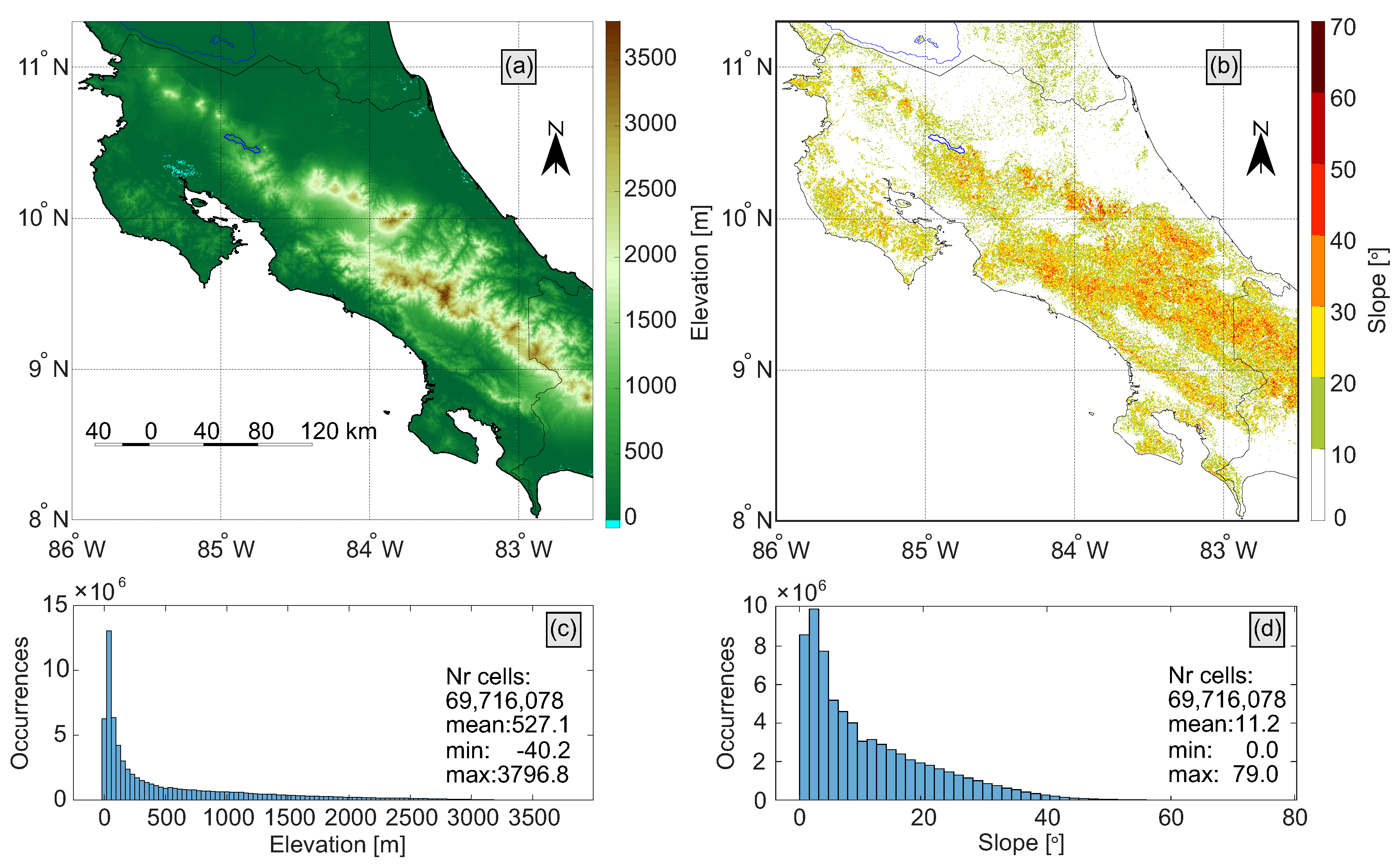
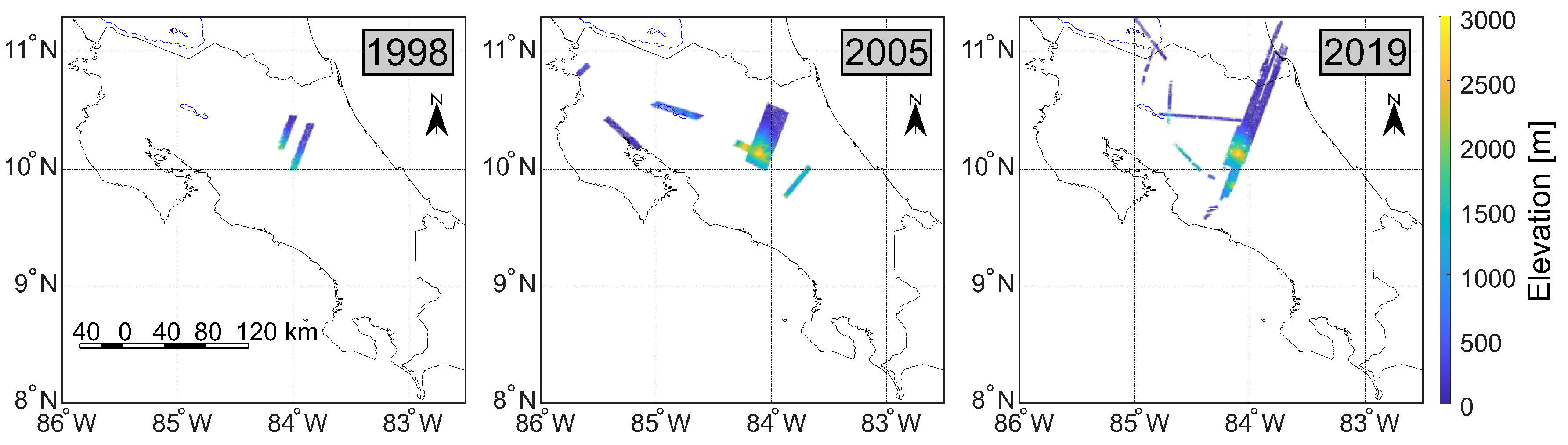
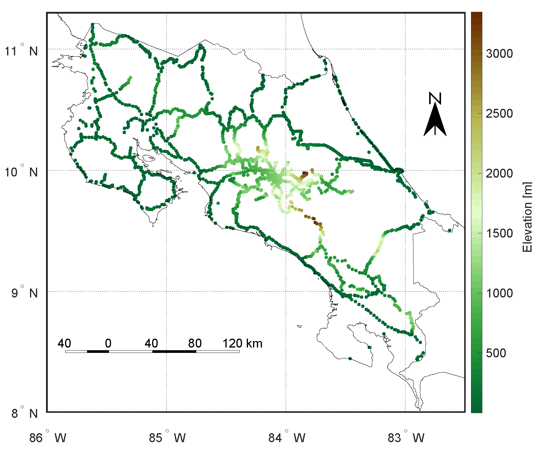
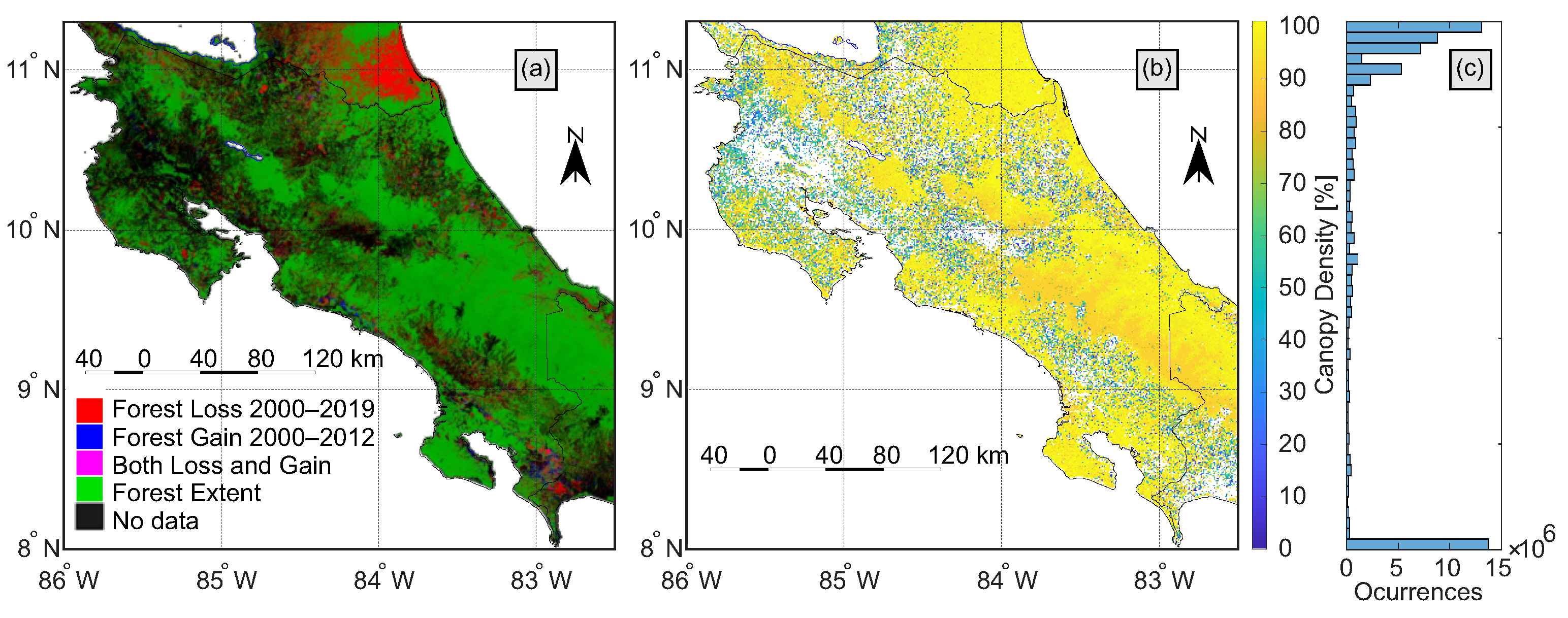
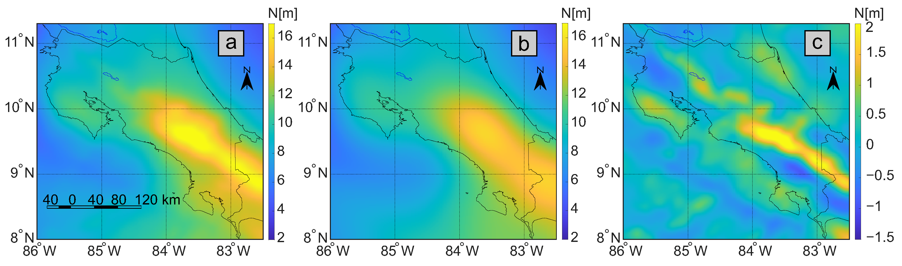
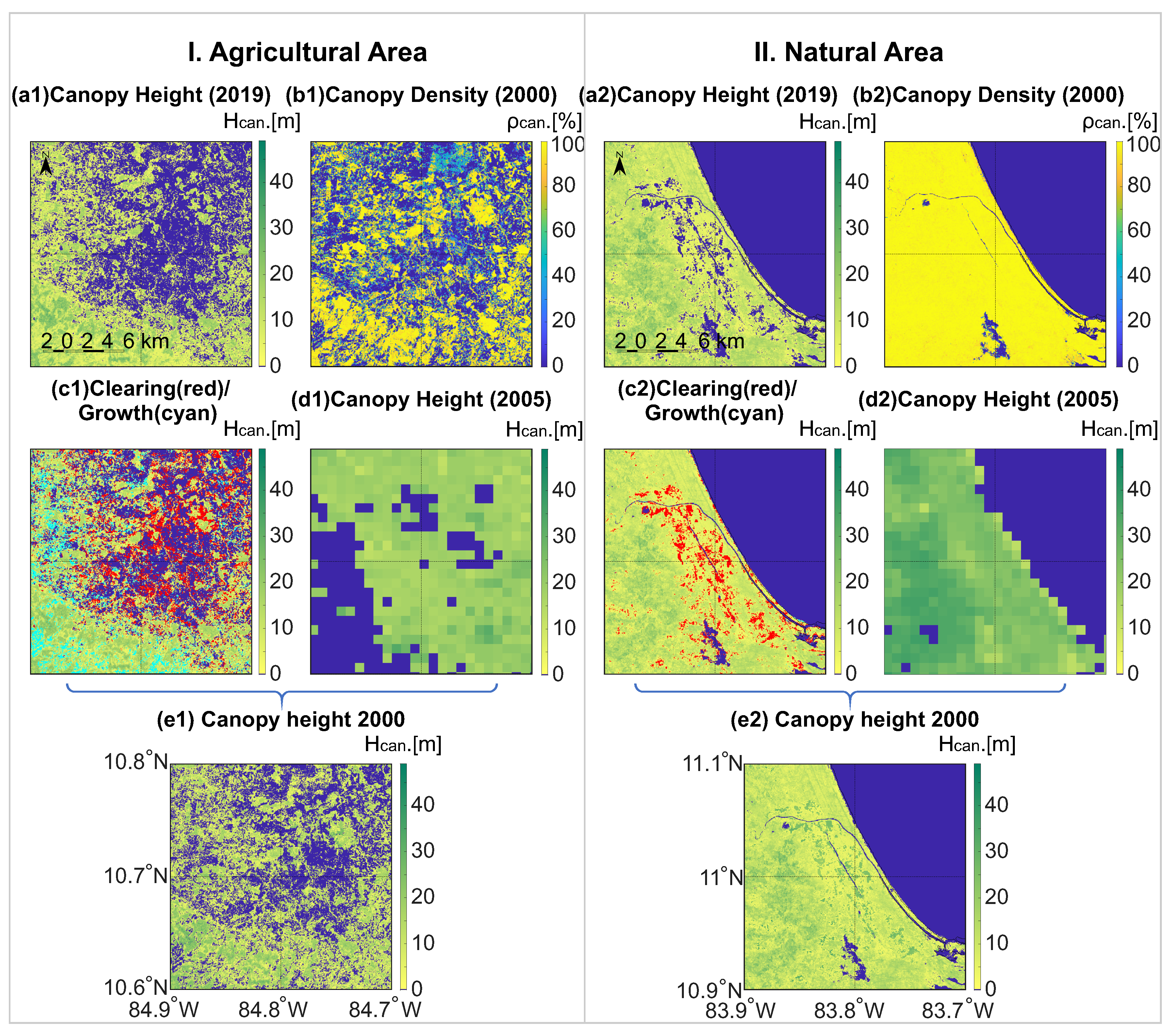
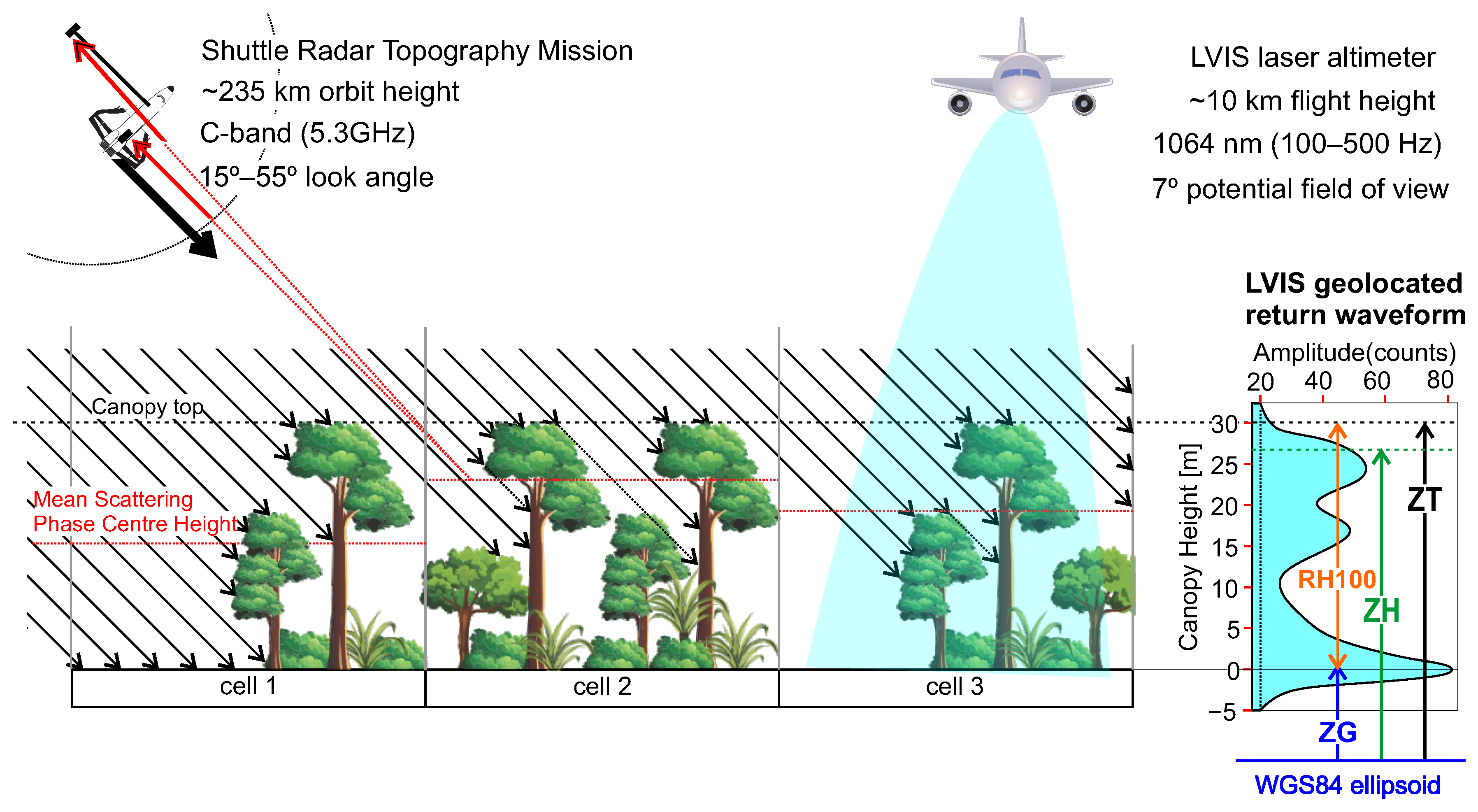
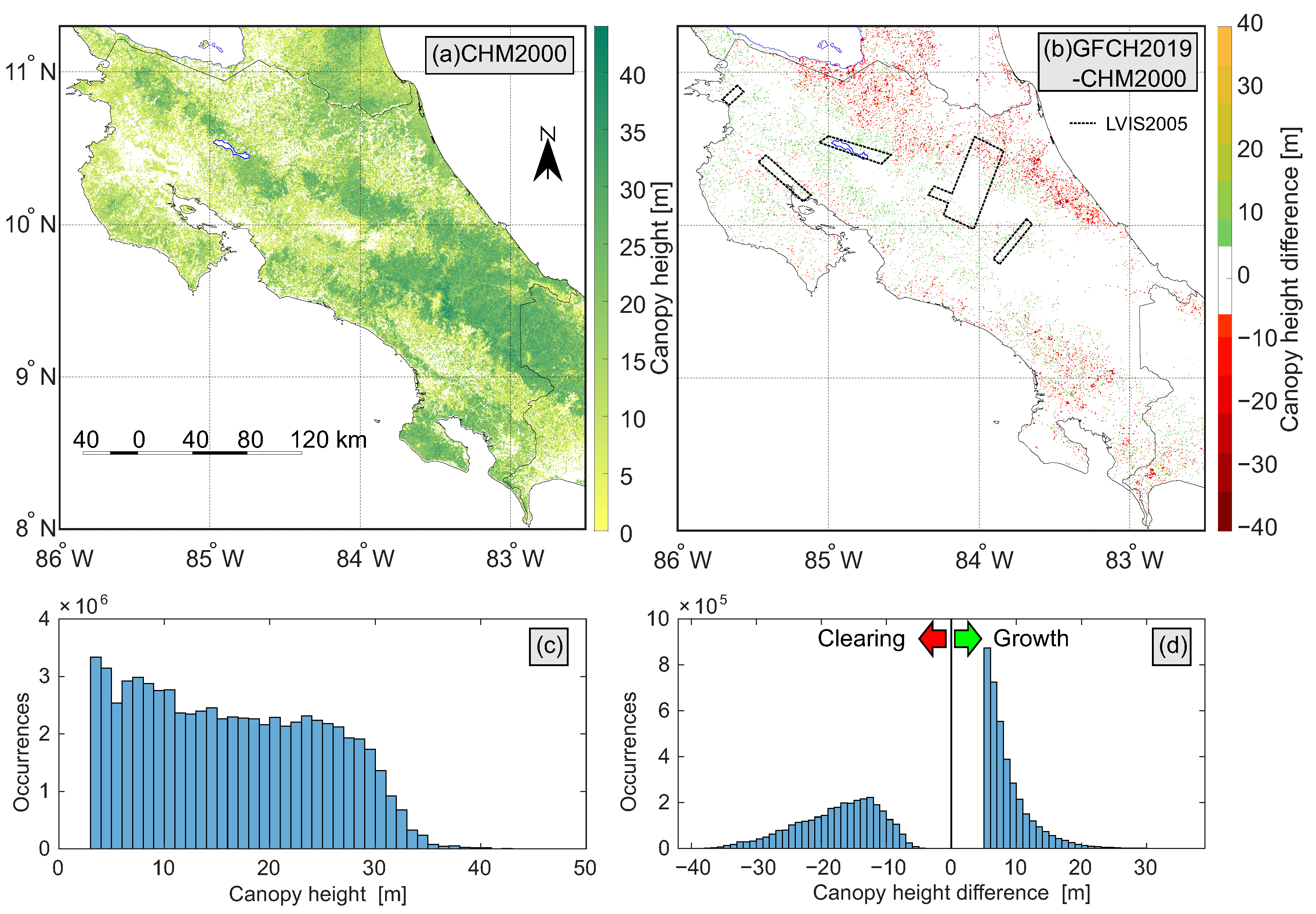
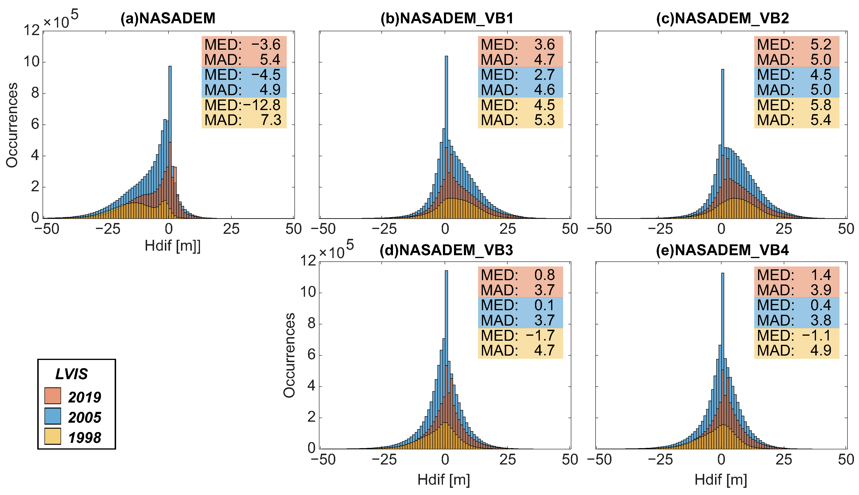
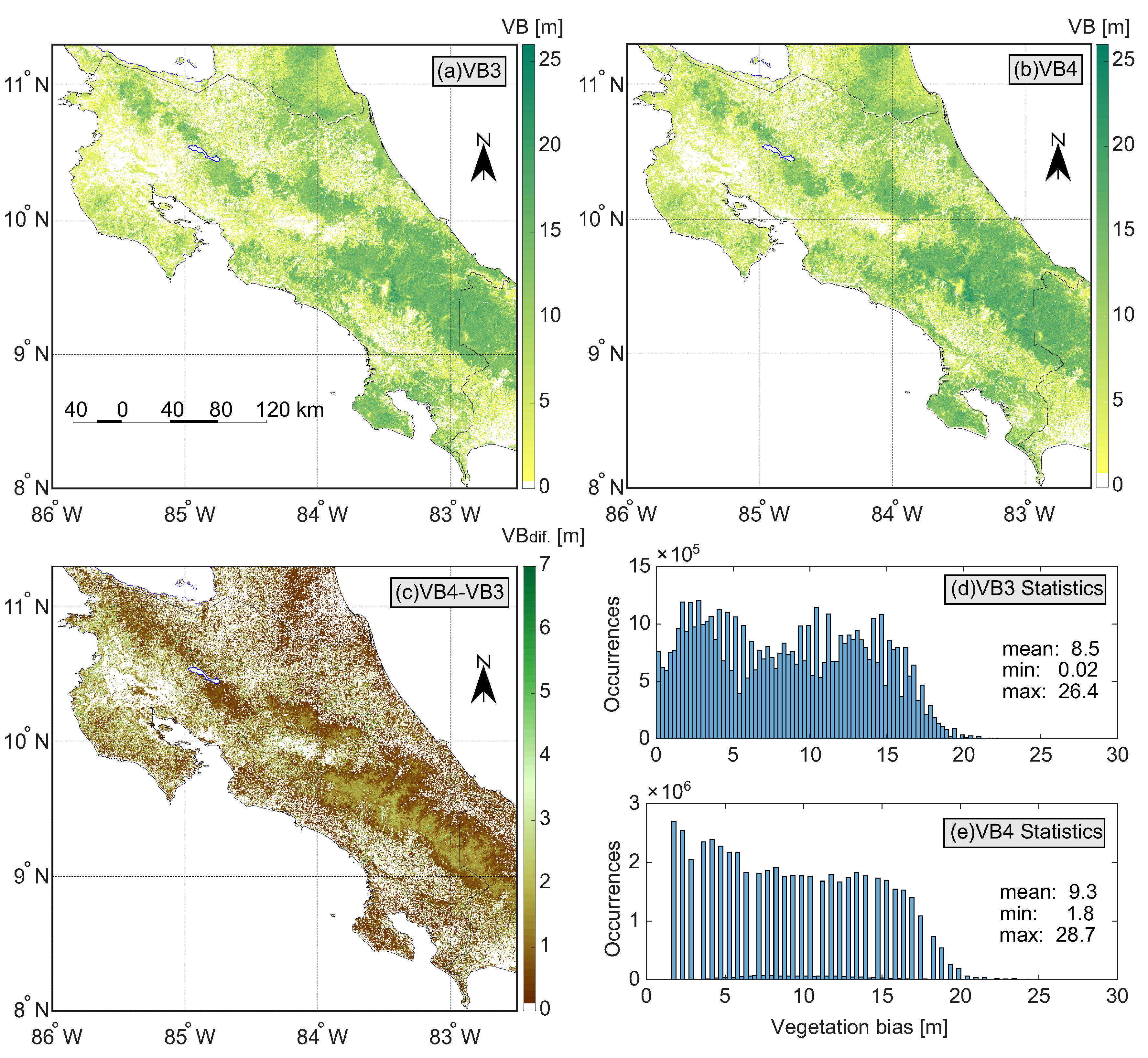
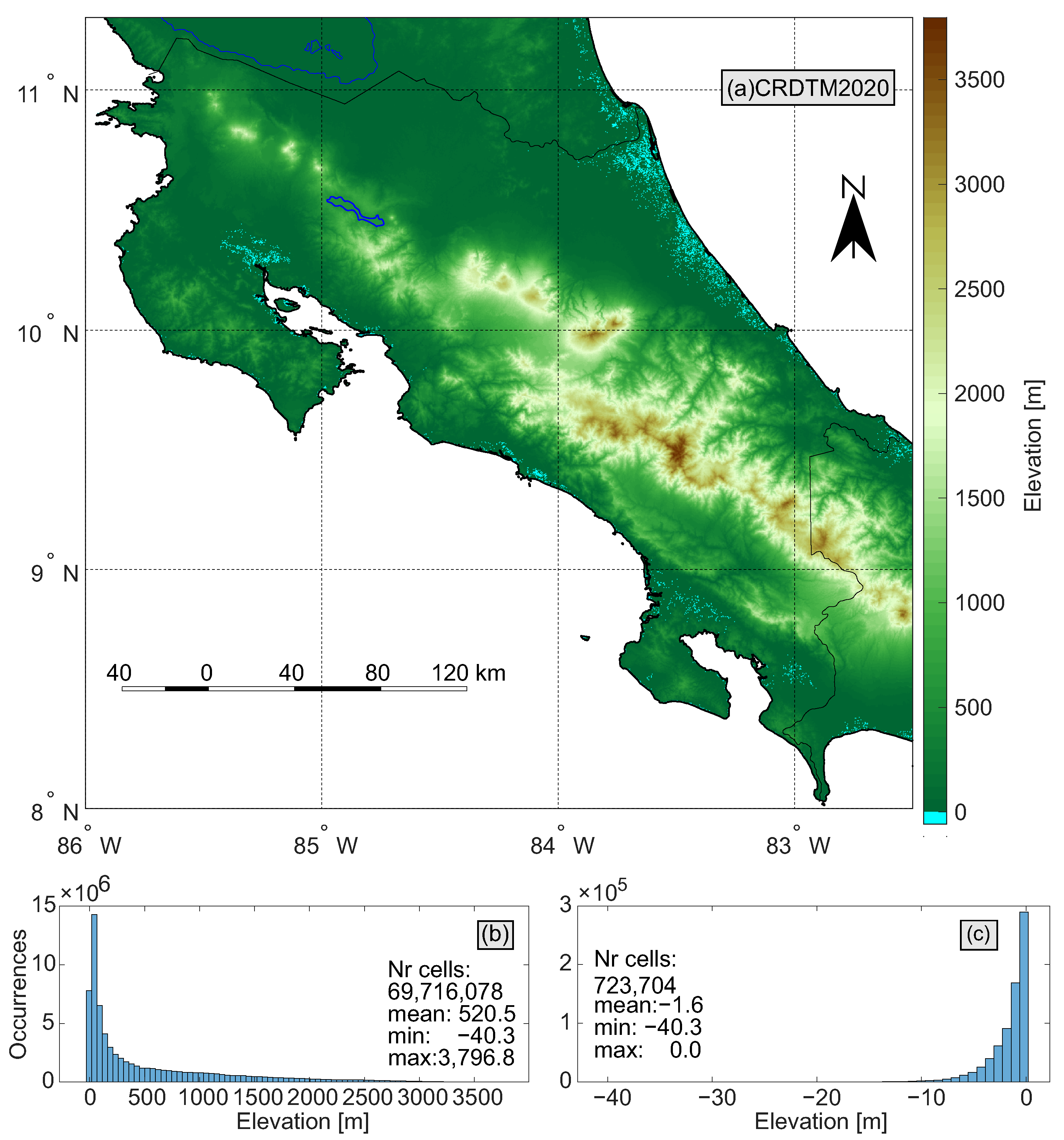
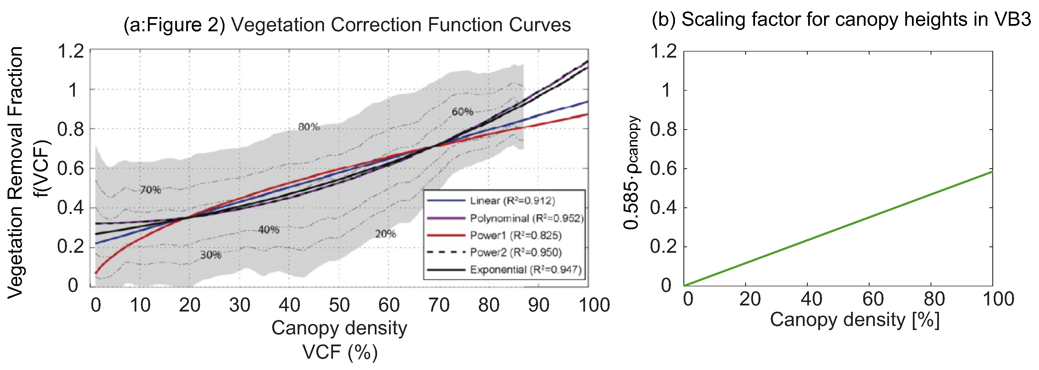
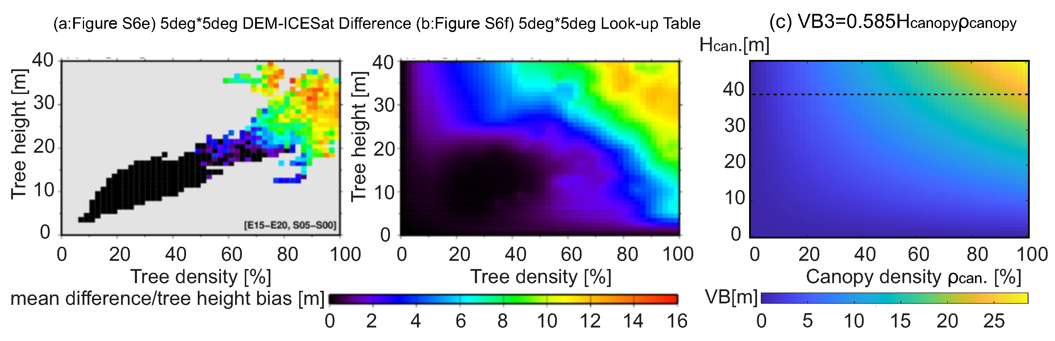
Table 1.
Overview of the publicly available global Digital Terrain Models (DTM) and Digital Surface Models (DSM) evaluated for Costa Rica in this study. The column “Mission” here indicates the remote sensing mission that was the principal data source used in the DEM in the study area (latitudes below 20°).
| DEM | Mesh Size | Mission | DTM/DSM | Provider | Reference |
|---|---|---|---|---|---|
| MERIT DEM | 3″ ≈ 90 | SRTM | DTM | Univ. of Tokyo [4] | WGS84/EGM96 geoid |
| BEST DEM | 3″ ≈ 90 | SRTM | DTM | bris.ac.uk [27] | WGS84/EGM96 geoid |
| NASADEM | 1″ ≈ 30 | SRTM | DSM | LP DAAC/USGS [19] | WGS84/EGM96 geoid |
| SRTMGL1 v003 | 1″ ≈ 30 | SRTM | DSM | LP DAAC/USGS [18] | WGS84/EGM96 geoid |
| SRTM v4.1 | 3″ ≈ 90 | SRTM | DSM | CGIAR-CSI [26] | WGS84/EGM96 geoid |
| SRTM3 v2.1 | 3″ ≈ 90 | SRTM | DSM | USGS [25] | WGS84/EGM96 geoid |
| TanDEM-X | 3″ ≈ 90 | TDX | DSM | DLR [28] | WGS84/WGS84 ellipsoid |
| ASTER GDEM v3 | 1″ ≈ 30 | Terra | DSM | NASA/METI [24] | WGS84/EGM96 geoid |
| AW3D30 v3.1 | 1″ ≈ 30 | ALOS | DSM | JAXA [22,23] | WGS84/EGM96 geoid |
Table 2.
List of parameters from the Laser Vegetation Imaging Sensor (LVIS) Classic L1B Geolocated Waveforms and LVIS Classic L2 Geolocated Surface Elevation and Canopy Height Product used in the study.
Table 2.
List of parameters from the Laser Vegetation Imaging Sensor (LVIS) Classic L1B Geolocated Waveforms and LVIS Classic L2 Geolocated Surface Elevation and Canopy Height Product used in the study.
| Parameter | Description | Units |
|---|---|---|
| SHOTNUMBER | LVIS shot number for the unique identification of laser shots | N/A |
| GLON | Longitude of the lowest detected mode within the waveform | |
| GLAT | Latitude of the lowest detected mode within the waveform | |
| ZG | Mean elevation of the lowest detected mode within the waveform | m |
| ZH * | Mean elevation of the highest detected mode within the waveform | m |
| ZT | Elevation of the highest detected signal | m |
| RH85 * | Height (relative to ZG) at which 85% of the waveform energy occurs | m |
| RH90 * | Height (relative to ZG) at which 90% of the waveform energy occurs | m |
| RH95 * | Height (relative to ZG) at which 95% of the waveform energy occurs | m |
| RH100 | Height (relative to ZG) at which 100% of the waveform energy occurs | m |
* These parameters are only available in the LVIS2019 data files.
Table 3.
Statistics of the differences between LVIS data from 2019, 2005, and 1998 and heights interpolated for original NASADEM and NASADEM corrected by four vegetable bias models. The statistics is provided in terms of the mean difference, Standard Deviation (STD*) for differences without outliers larger than ±50, Median Absolute Difference (MAD), 25th empirical quartile Q1, the Median (MED) or the 50th empirical quartile Q2, the 75th empirical quartile Q3, and percentages of points having absolute differences below certain thresholds.
| Mean | STD* | MAD | Q1 | Q2(MED) | Q3 | Points with Absolute Difference (%) | ||||
|---|---|---|---|---|---|---|---|---|---|---|
| (m) | (m) | (m) | (m) | (m) | (m) | ≤5 m | ≤10 m | ≤15 m | ≤20 m | |
| LVIS2019: 5,195,224 points | ||||||||||
| NASADEM | −5.6 | 9.3 | 5.4 | −11.7 | −3.6 | 0.7 | 50% | 69% | 82% | 91% |
| NASADEM_VB1 | 5.6 | 8.9 | 4.7 | 0.1 | 3.6 | 10.0 | 48% | 72% | 86% | 93% |
| NASADEM_VB2 | 6.9 | 9.1 | 5.0 | 0.7 | 5.2 | 11.7 | 42% | 67% | 83% | 92% |
| NASADEM_VB3 | 0.9 | 7.9 | 3.7 | −3.2 | 0.8 | 4.3 | 59% | 83% | 93% | 97% |
| NASADEM_VB4 | 1.7 | 8.0 | 3.9 | −2.6 | 1.4 | 5.3 | 57% | 82% | 92% | 97% |
| LVIS2005: 9,280,657 points | ||||||||||
| NASADEM | −7.2 | 9.5 | 4.9 | −12.4 | −4.5 | −0.3 | 49% | 68% | 80% | 89% |
| NASADEM_VB1 | 4.2 | 8.7 | 4.6 | −0.8 | 2.7 | 9.1 | 51% | 74% | 88% | 94% |
| NASADEM_VB2 | 5.7 | 8.9 | 5.0 | 0.2 | 4.5 | 10.8 | 45% | 70% | 85% | 93% |
| NASADEM_VB3 | −0.5 | 7.9 | 3.7 | −4.0 | 0.1 | 3.4 | 60% | 84% | 93% | 97% |
| NASADEM_VB4 | 0.3 | 8.0 | 3.8 | −3.2 | 0.4 | 4.5 | 59% | 83% | 93% | 97% |
| LVIS1998: 2,570,730 points | ||||||||||
| NASADEM | −13.6 | 9.9 | 7.3 | −19.7 | −12.8 | −5.2 | 24% | 39% | 58% | 76% |
| NASADEM_VB1 | 4.4 | 9.0 | 5.3 | −0.5 | 4.5 | 10.1 | 41% | 69% | 87% | 95% |
| NASADEM_VB2 | 5.4 | 9.1 | 5.4 | 0.4 | 5.8 | 11.2 | 36% | 65% | 85% | 94% |
| NASADEM_VB3 | −3.1 | 8.5 | 4.7 | −7.4 | −1.7 | 2.3 | 53% | 79% | 91% | 96% |
| NASADEM_VB4 | −2.5 | 8.7 | 4.9 | −7.0 | −1.1 | 3.2 | 51% | 79% | 91% | 96% |
| Levelling dataset: 2233 points | ||||||||||
| NASADEM | −3.5 | 10.0 | 3.7 | −6.6 | −2.7 | 0.8 | 57% | 78% | 85% | 90% |
| NASADEM_VB1 | 0.3 | 10.4 | 4.1 | −4.4 | −0.9 | 4.0 | 56% | 77% | 85% | 90% |
| NASADEM_VB2 | 2.0 | 10.7 | 4.7 | −3.4 | 0.7 | 6.3 | 53% | 75% | 84% | 89% |
| NASADEM_VB3 | −1.3 | 10.1 | 3.8 | −5.0 | −1.5 | 2.5 | 59% | 79% | 86% | 91% |
| NASADEM_VB4 | −0.3 | 10.0 | 3.9 | −4.2 | −0.7 | 3.7 | 59% | 79% | 86% | 91% |
Table 4.
Statistical analysis of the differences between LVIS lowest heights (ZG) and the heights of the nine DEMs interpolated on the same locations. The statistics is provided in terms of the mean difference, Standard Deviation (STD*) for differences without outliers larger than ±50, minimum and maximum differences (min/max), Median Absolute Difference (MAD), 25th empirical quartile Q1, the Median (MED) or the 50th empirical quartile Q2, the 75th empirical quartile Q3, and percentages of points having absolute differences below certain thresholds. STD* marked in grey indicates that differences for those DEMs are not normally distributed, and these values are not appropriate metrics for their evaluation. They are provided as they may be of interest, e.g., for comparison to other studies.
| Mean | STD* | min/max | MAD | Q1 | Q2(MED) | Q3 | Points with Absolute Difference (%) | ||||
|---|---|---|---|---|---|---|---|---|---|---|---|
| (m) | (m) | (m) | (m) | (m) | (m) | (m) | ≤5 m | ≤10 m | ≤15 m | ≤20 m | |
| LVIS2019: 5,195,224 points | |||||||||||
| CRDTM2020 | 0.9 | 7.9 | −248/250 | 3.7 | −3.2 | 0.8 | 4.3 | 59% | 83% | 93% | 97% |
| MERIT | −0.7 | 9.6 | −199/259 | 4.2 | −5.1 | 0.0 | 3.4 | 56% | 78% | 88% | 93% |
| BEST | −3.9 | 10.9 | −196/260 | 6.0 | −10.4 | −4.2 | 1.7 | 36% | 63% | 79% | 87% |
| NASADEM | −5.6 | 9.3 | −257/250 | 5.4 | −11.7 | −3.6 | 0.7 | 50% | 69% | 82% | 91% |
| SRTMGL1 | −8.6 | 9.4 | −190/263 | 5.5 | −14.9 | −6.8 | −2.5 | 37% | 58% | 72% | 83% |
| SRTM4 | −8.3 | 10.7 | −208/250 | 6.2 | −14.9 | −6.4 | −1.7 | 38% | 59% | 74% | 84% |
| SRTM3 | −8.3 | 10.7 | −208/250 | 6.2 | −14.9 | −6.3 | −1.7 | 38% | 59% | 74% | 84% |
| TanDEM-X | −6.0 | 14.5 | −249/338 | 7.3 | −14.1 | −3.9 | 1.0 | 36% | 55% | 68% | 77% |
| ASTER | −4.8 | 13.5 | −181/260 | 7.9 | −13.6 | −2.4 | 3.7 | 36% | 59% | 73% | 83% |
| AW3D30 | −8.6 | 9.5 | −213/247 | 5.6 | −15.0 | −6.4 | −2.3 | 40% | 61% | 74% | 85% |
| LVIS2005: 9,280,657 points | |||||||||||
| CRDTM2020 | −0.5 | 7.9 | −186/276 | 3.7 | −4.0 | 0.1 | 3.4 | 60% | 84% | 93% | 97% |
| MERIT | −2.6 | 10.2 | −220/282 | 4.7 | −6.8 | −1.5 | 2.7 | 52% | 75% | 86% | 92% |
| BEST | −5.8 | 11.0 | −222/286 | 6.2 | −11.9 | −5.8 | 0.7 | 32% | 59% | 81% | 89% |
| NASADEM | −7.2 | 9.5 | −199/266 | 4.9 | −12.4 | −4.5 | −0.3 | 49% | 68% | 80% | 89% |
| SRTMGL1 | −9.8 | 9.3 | −205/264 | 4.7 | −14.9 | −7.2 | −3.1 | 35% | 60% | 74% | 85% |
| SRTM4 | −9.7 | 10.7 | −231/272 | 5.1 | −15.2 | −7.1 | −2.8 | 34% | 59% | 74% | 83% |
| SRTM3 | −9.7 | 10.7 | −211/272 | 5.1 | −15.2 | −7.1 | −2.8 | 34% | 59% | 74% | 83% |
| TanDEM-X | −7.6 | 15.3 | −237/205 | 7.9 | −16.1 | −5.6 | 0.2 | 32% | 51% | 65% | 75% |
| ASTER | −5.0 | 12.4 | −203/273 | 7.2 | −11.7 | −3.3 | 2.9 | 36% | 62% | 77% | 86% |
| AW3D30 | −10.0 | 9.5 | −204/280 | 4.8 | −15.4 | −7.2 | −2.9 | 36% | 60% | 74% | 84% |
| LVIS1998: 2,570,730 points | |||||||||||
| CRDTM2020 | −3.1 | 8.5 | −258/380 | 4.7 | −7.4 | −1.7 | 2.3 | 53% | 79% | 91% | 96% |
| MERIT | −6.1 | 10.8 | −229/384 | 6.2 | −11.5 | −3.9 | 1.5 | 44% | 68% | 81% | 89% |
| BEST | −6.0 | 10.7 | −229/388 | 5.7 | −10.9 | −4.7 | 0.6 | 36% | 63% | 79% | 87% |
| NASADEM | −13.6 | 9.9 | −258/369 | 7.3 | −19.7 | −12.8 | −5.2 | 24% | 39% | 58% | 76% |
| SRTMGL1 | −16.6 | 9.7 | −230/370 | 7.2 | −22.7 | −15.6 | −8.4 | 11% | 30% | 47% | 66% |
| SRTM4 | −16.6 | 10.9 | −238/374 | 7.9 | −23.1 | −14.9 | −7.2 | 13% | 34% | 50% | 66% |
| SRTM3 | −16.5 | 10.9 | −238/374 | 7.9 | −23.1 | −14.9 | −7.2 | 13% | 34% | 50% | 66% |
| TanDEM-X | −10.4 | 14.0 | −300/345 | 7.6 | −18.4 | −7.4 | −1.1 | 33% | 51% | 64% | 74% |
| ASTER | −11.4 | 13.5 | −181/372 | 9.7 | −20.3 | −10.5 | −0.9 | 24% | 44% | 60% | 73% |
| AW3D30 | −17.0 | 9.9 | −241/361 | 7.4 | −23.5 | −16.3 | −8.7 | 11% | 29% | 45% | 63% |
| Levelling dataset: 2,233 points | |||||||||||
| CRDTM2020 | −1.2 | 10.0 | −162/183 | 3.8 | −4.9 | −1.5 | 2.6 | 59% | 79% | 86% | 91% |
| MERIT | −0.9 | 10.6 | −161/187 | 4.2 | −5.5 | −1.4 | 3.1 | 54% | 78% | 86% | 89% |
| BEST | −7.7 | 11.4 | −165/181 | 6.0 | −14.3 | −8.3 | −2.2 | 25% | 51% | 73% | 86% |
| NASADEM | −3.5 | 10.0 | −169/183 | 3.7 | −6.6 | −2.7 | 0.8 | 57% | 78% | 85% | 90% |
| SRTMGL1 | −4.7 | 10.2 | −205/187 | 3.8 | −8.2 | −4.1 | −0.7 | 48% | 74% | 84% | 89% |
| SRTM4 | −4.5 | 10.6 | −171/186 | 3.8 | −8.2 | −4.1 | −0.5 | 47% | 75% | 84% | 89% |
| SRTM3 | −4.6 | 10.6 | −165/186 | 3.8 | −8.1 | −4.1 | −0.5 | 47% | 75% | 84% | 89% |
| TanDEM-X | −3.3 | 12.1 | −162/187 | 4.3 | −7.2 | −2.1 | 1.5 | 53% | 71% | 80% | 86% |
| ASTER | −0.7 | 12.3 | −166/182 | 6.0 | −6.7 | −0.6 | 5.3 | 43% | 68% | 80% | 87% |
| AW3D30 | −4.7 | 10.3 | −162/188 | 3.7 | −8.0 | −4.0 | −0.5 | 49% | 75% | 84% | 89% |
Table 5.
Statistics of the differences between LVIS lowest heights (ZG) and the heights of the nine DEMs interpolated on the same locations. Comparison with TanDEM-X was performed directly in terms of ellipsoidal heights, others as heights above the EGM96 geoid. The statistics is provided in terms of the mean difference, Standard Deviation (STD*) for differences without outliers larger than ±50, minimum and maximum differences (min/max), Median Absolute Difference (MAD), 25th empirical quartile Q1, the Median (MED) or the 50th empirical quartile Q2, and 75th empirical quartile Q3.
| Points above Bare-Earth | Points above Vegetation | ||||||||||||
|---|---|---|---|---|---|---|---|---|---|---|---|---|---|
| mean | STD* | min/max | MAD | Q1 | MED | Q3 | mean | STD* | MAD | Q1 | MED | Q3 | |
| (m) | (m) | (m) | (m) | (m) | (m) | (m) | (m) | (m) | (m) | (m) | (m) | (m) | |
| LVIS2019: 5,195,224 points, 31.6% bare-earth, 68.4% vegetated | |||||||||||||
| CRDTM2020 | 2.3 | 6.0 | −181/217 | 2.1 | −0.1 | 1.7 | 4.2 | 0.3 | 8.5 | 4.5 | −4.7 | 0.0 | 4.3 |
| MERIT | 1.6 | 6.4 | −198/235 | 2.2 | −1.0 | 0.7 | 3.5 | −1.8 | 10.6 | 5.2 | −7.4 | −1.4 | 3.3 |
| BEST | −3.1 | 8.9 | −196/235 | 4.2 | −7.9 | −3.7 | 1.0 | −4.2 | 11.6 | 6.9 | −11.9 | −4.5 | 2.0 |
| NASADEM | −0.4 | 5.4 | −194/206 | 2.1 | −2.0 | 0.6 | 2.6 | −8.1 | 9.5 | 6.4 | −14.6 | −7.5 | −1.5 |
| SRTMGL1 | −3.4 | 5.9 | −129/207 | 2.8 | −5.5 | −2.7 | 0.1 | −10.8 | 9.5 | 6.3 | −17.5 | −10.2 | −4.4 |
| SRTM4 | −3.0 | 6.8 | −208/226 | 2.9 | −5.6 | −2.2 | 0.6 | −10.8 | 11.1 | 6.8 | −18.1 | −10.0 | −4.0 |
| SRTM3 | −3.0 | 6.8 | −208/226 | 2.9 | −5.6 | −2.2 | 0.6 | −10.8 | 11.1 | 6.8 | −18.1 | −10.0 | −4.0 |
| TanDEM-X | −1.5 | 12.0 | −207/307 | 4.3 | −6.3 | −0.6 | 2.3 | −7.9 | 15.2 | 8.2 | −17.1 | −6.5 | 0.2 |
| ASTER | 0.6 | 10.3 | −146/229 | 4.7 | −3.0 | 0.8 | 5.9 | −7.3 | 14.0 | 9.4 | −17.1 | −6.3 | 2.2 |
| AW3D30 | −3.1 | 5.7 | −188/212 | 2.9 | −5.2 | −2.4 | 0.6 | −11.2 | 9.6 | 6.6 | −18.2 | −10.4 | −4.4 |
| LVIS2005: 9,280,657 points, 16.4% bare-earth, 83.6% vegetated | |||||||||||||
| CRDTM2020 | 0.5 | 3.6 | −116/92 | 0.9 | −0.7 | 0.3 | 1.0 | −0.7 | 8.5 | 4.4 | −4.9 | −0.4 | 4.0 |
| MERIT | −0.7 | 3.9 | −143/95 | 0.9 | −2.2 | −1.3 | −0.4 | −3.0 | 11.0 | 5.7 | −8.3 | −1.9 | 3.3 |
| BEST | −7.9 | 6.2 | −150/86 | 2.3 | −12.0 | −9.9 | −4.6 | −5.4 | 11.6 | 6.7 | −11.7 | −5.0 | 1.6 |
| NASADEM | −0.4 | 3.0 | −116/92 | 0.8 | −1.3 | 0.2 | 0.5 | −8.5 | 9.8 | 5.8 | −14.2 | −6.4 | −1.5 |
| SRTMGL1 | −3.5 | 3.0 | −121/80 | 0.7 | −4.5 | −2.8 | −2.5 | −11.0 | 9.6 | 5.6 | −16.6 | −8.9 | −4.3 |
| SRTM4 | −3.5 | 3.5 | −167/94 | 0.9 | −4.6 | −2.8 | −2.5 | −11.0 | 11.3 | 6.2 | −17.2 | −8.9 | −3.9 |
| SRTM3 | −3.5 | 3.5 | −149/94 | 1.0 | −4.6 | −2.8 | −2.5 | −11.0 | 11.3 | 6.2 | −17.2 | −8.9 | −3.9 |
| TanDEM-X | −2.3 | 13.0 | −201/115 | 4.2 | −6.0 | −1.0 | 2.2 | −8.6 | 15.5 | 8.4 | −17.7 | −7.1 | −0.3 |
| ASTER | 0.1 | 6.9 | −131/106 | 2.5 | −3.7 | 1.2 | 2.0 | −6.0 | 13.0 | 8.2 | −13.6 | −4.8 | 3.0 |
| AW3D30 | −3.3 | 3.1 | −112/89 | 0.7 | −4.1 | −2.8 | −2.5 | −11.3 | 9.8 | 5.9 | −17.2 | −9.2 | −4.3 |
| LVIS1998: 2,570,730 points, 0.3% bare-earth, 99.7% vegetated | |||||||||||||
| CRDTM2020 | 1.5 | 3.5 | −46/25 | 1.7 | −0.5 | 1.0 | 2.9 | −3.1 | 8.6 | 4.7 | −7.4 | −1.7 | 2.3 |
| MERIT | 1.3 | 3.7 | −67/31 | 2.2 | −1.1 | 0.7 | 3.5 | −6.1 | 10.8 | 6.2 | −11.6 | −3.9 | 1.5 |
| BEST | −2.3 | 4.6 | −67/28 | 2.3 | −4.7 | −2.6 | −0.2 | −6.0 | 10.7 | 5.7 | −10.9 | −4.7 | 0.6 |
| NASADEM | −0.5 | 2.4 | −66/16 | 1.3 | −1.8 | −0.4 | 0.8 | −13.6 | 9.9 | 7.2 | −19.8 | −12.9 | −5.2 |
| SRTMGL1 | −4.3 | 2.5 | −73/11 | 1.3 | −5.6 | −4.3 | −3.0 | −16.7 | 9.7 | 7.1 | −22.7 | −15.7 | −8.4 |
| SRTM4 | −4.5 | 2.8 | −77/20 | 1.3 | −5.7 | −4.5 | −3.2 | −16.6 | 10.9 | 7.9 | −23.1 | −14.9 | −7.3 |
| SRTM3 | −4.5 | 2.8 | −77/20 | 1.3 | −5.8 | −4.5 | −3.2 | −16.6 | 10.9 | 7.9 | −23.1 | −14.9 | −7.3 |
| TanDEM-X | −1.7 | 4.6 | −86/40 | 1.4 | −2.7 | −1.2 | 0.1 | −10.5 | 14.1 | 7.7 | −18.4 | −7.4 | −1.1 |
| ASTER | 3.4 | 5.7 | −56/30 | 3.3 | 0.3 | 3.9 | 7.0 | −11.4 | 13.5 | 9.7 | −20.3 | −10.5 | −1.0 |
| AW3D30 | −4.8 | 3.4 | −43/41 | 1.3 | −5.9 | −4.6 | −3.4 | −17.1 | 9.9 | 7.4 | −23.6 | −16.4 | −8.8 |
| Levelling dataset: 2233 points, 54.4% bare-earth, 45.6% vegetated | |||||||||||||
| CRDTM2020 | −2.6 | 7.2 | −162/183 | 2.6 | −4.5 | −2.0 | 0.8 | −0.1 | 11.8 | 5.1 | −5.8 | −0.7 | 4.5 |
| MERIT | −2.3 | 8.1 | −161/187 | 3.3 | −5.5 | −2.3 | 1.2 | 0.8 | 13.0 | 5.7 | −5.6 | 0.3 | 5.9 |
| BEST | −9.9 | 9.2 | −165/178 | 5.0 | −14.9 | −10.1 | −4.9 | −5.8 | 12.8 | 6.8 | −13.4 | −6.4 | 0.1 |
| NASADEM | −2.6 | 7.3 | −162/183 | 2.7 | −4.6 | −2.0 | 0.8 | −4.5 | 12.4 | 5.1 | −9.6 | −4.1 | 0.7 |
| SRTMGL1 | −4.1 | 7.5 | −161/187 | 2.9 | −6.5 | −3.7 | −0.7 | −5.5 | 12.6 | 5.2 | −10.9 | −5.0 | −0.6 |
| SRTM4 | −3.8 | 8.0 | −161/186 | 2.9 | −6.3 | −3.6 | −0.6 | −5.5 | 13.0 | 5.3 | −10.9 | −5.0 | −0.2 |
| SRTM3 | −3.8 | 8.0 | −161/186 | 2.9 | −6.3 | −3.6 | −0.5 | −5.5 | 13.0 | 5.3 | −10.9 | −5.1 | −0.3 |
| TanDEM-X | −2.7 | 9.7 | −162/187 | 3.1 | −4.8 | −1.3 | 1.4 | −4.1 | 14.4 | 6.0 | −10.8 | −3.6 | 1.6 |
| ASTER | 0.7 | 10.2 | −153/180 | 4.9 | −4.3 | 0.8 | 5.6 | −2.5 | 14.3 | 7.5 | −10.3 | −3.0 | 4.8 |
| AW3D30 | −3.9 | 7.7 | −162/188 | 2.8 | −6.0 | −3.7 | −0.5 | −5.7 | 12.6 | 5.2 | −11.4 | −4.7 | −0.5 |
Publisher’s Note: MDPI stays neutral with regard to jurisdictional claims in published maps and institutional affiliations. |
© 2022 by the authors. Licensee MDPI, Basel, Switzerland. This article is an open access article distributed under the terms and conditions of the Creative Commons Attribution (CC BY) license (https://creativecommons.org/licenses/by/4.0/).
Share and Cite
MDPI and ACS Style
Pimenova, O.; Roberts, C.; Rizos, C. Regional “Bare-Earth” Digital Terrain Model for Costa Rica Based on NASADEM Corrected for Vegetation Bias. Remote Sens. 2022, 14, 2421. https://0-doi-org.brum.beds.ac.uk/10.3390/rs14102421
AMA Style
Pimenova O, Roberts C, Rizos C. Regional “Bare-Earth” Digital Terrain Model for Costa Rica Based on NASADEM Corrected for Vegetation Bias. Remote Sensing. 2022; 14(10):2421. https://0-doi-org.brum.beds.ac.uk/10.3390/rs14102421
Chicago/Turabian StylePimenova, Olga, Craig Roberts, and Chris Rizos. 2022. "Regional “Bare-Earth” Digital Terrain Model for Costa Rica Based on NASADEM Corrected for Vegetation Bias" Remote Sensing 14, no. 10: 2421. https://0-doi-org.brum.beds.ac.uk/10.3390/rs14102421
Note that from the first issue of 2016, this journal uses article numbers instead of page numbers. See further details here.