
GapLoss: A Loss Function for Semantic Segmentation of Roads in Remote Sensing Images


1
School of Computer Science, Chengdu University, Chengdu 610106, China
2
Key Laboratory of Pattern Recognition and Intelligent Information Processing, Institutions of Higher Education of Sichuan Province, Chengdu University, Chengdu 610106, China
3
School of Resources and Environment, University of Electronic Science and Technology of China, Chengdu 611731, China
*
Author to whom correspondence should be addressed.
Remote Sens. 2022, 14(10), 2422; https://0-doi-org.brum.beds.ac.uk/10.3390/rs14102422
Submission received: 12 March 2022
/
Revised: 29 April 2022
/
Accepted: 17 May 2022
/
Published: 18 May 2022
(This article belongs to the Section AI Remote Sensing)
Abstract
:At present, road continuity is a major challenge, and it is difficult to extract the centerline vector of roads, especially when the road view is obstructed by trees or other structures. Most of the existing research has focused on optimizing the available deep-learning networks. However, the segmentation accuracy is also affected by the loss function. Currently, little research has been published on road segmentation loss functions. To resolve this problem, an attention loss function named GapLoss that can be combined with any segmentation network was proposed. Firstly, a deep-learning network was used to obtain a binary prediction mask. Secondly, a vector skeleton was extracted from the prediction mask. Thirdly, for each pixel, eight neighboring pixels with the same value of the pixel were calculated. If the value was 1, then the pixel was identified as the endpoint. Fourth, according to the number of endpoints within a buffered range, each pixel in the prediction image was given a corresponding weight. Finally, the weighted average value of the cross-entropy of all the pixels in the batch was used as the final loss function value. We employed four well-known semantic segmentation networks to conduct comparative experiments on three large datasets. The results showed that, compared to other loss functions, the evaluation metrics after using GapLoss were nearly all improved. From the predicted image, the road prediction by GapLoss was more continuous, especially at intersections and when the road was obscured from view, and the road segmentation accuracy was improved.
1. Introduction
Roads are an indispensable element of human life and production activities, including navigation, traffic management, electronic map making, urban planning, and so on. In the field of surveying and mapping, roads are one of the main contents of geographic information data. Manually extracting road information from remote sensing images can meet the needs of most applications, but it is very labor-intensive, so many researchers have studied how to automate road extraction from remote sensing images.
In the early stages, automated road extraction methods primarily used the spectral features of remote sensing images supplemented by a morphological algorithm and then selected the appropriate threshold to segment the road. Laptev et al. [1] extracted roads from aerial images based on scale space and snakes. Maboudietal et al. [2] and Xue et al. [3] analyzed the spectral characteristics of water, vegetation, bare soil, buildings, cement roads, and asphalt roads using IKONOS satellite imagery, and while roads could be distinguished from some features, they were difficult to distinguish from, for example, a house, due to the spectra of roads and houses being too similar. Cai et al. [4] used a watershed algorithm based on region merging to segment roads, but the challenge of using this algorithm was that the threshold was difficult to determine, and the segmentation accuracy was dependent on the accuracy of the threshold.
Some researchers have applied machine-learning methods, such as random forest [5], SVM [6], Markov random fields classifier methods [7,8,9], mean-shift-based methods [10], and K-means clustering algorithms [11,12], to extract roads from remote sensing images, but the success of these methods depends on artificial design features, which is yet another challenge. Deep-learning technology has interrupted traditional research methods. Deep-learning networks, such as UNet [13], DeepLab family [14,15,16,17], SegNet [18], PSPNet [19], UNet++ [20], and MUNet [21], can extract features from an image and have proved to be more accurate and reliable than traditional machine learning, so they have become the main methods used in road segmentation research.
Many researchers have applied deep-learning technology to road segmentation using remote sensing images. Zhong et al. [22] applied FCN to extract roads and buildings in aerial images and achieved reliable results for the Massachusetts Roads Dataset [23]. Panboonyuen et al. [24] improved road segmentation results using a SegNet network and an ELU activation unit. Wei et al. [25] strengthened the weight of pixels near the label using a cross-entropy function to improve the accuracy of road recognition. Mattyus et al. [26] used ResNet as an encoder and a fully deconvolutional network as a decoder to acquire the topology of roads in aerial images. Gao et al. [27] proposed a multiple-feature pyramid network, which was similar to the RSRCNN. Zhang et al. [28] proposed a deep residual UNet to perform road extraction. Xu et al. [29] proposed a network named GL-Dense-UNet to extract roads. D-LinkNet [30] was selected as the best network solution in the 2018 DeepGlobe Road Extraction Challenge [31], and the second-best solution in the challenge [32] used ResNet-34 pretrained on ImageNet as its encoder and a decoder adapted from a “vanilla” UNet. A weakly supervised learning method for global-scale road extraction was proposed in [33]. Wu et al. [34] used weakly labeled data to extract roads. Wang et al. [35] proposed a coord-dense-global model (CDG) that used DenseNet, a coordconv module, and a global attention module to construct a road map from remote sensing imagery.
The accuracy of the segmentation results is determined by both the network model and the applied loss function [36], but there have been few achievements to provide evidence. Cross-entropy [37] has been the most widely used loss function in semantic segmentations of images; the other loss functions have been designed for unbalanced datasets, such as focal loss [38], dice loss [39], Tversky loss [40], log-cosh dice loss [41], and generalized dice loss [42], and they have not been capable of accurate road continuity, as they were not designed for linear object recognition.
There are very few loss functions designed for road extraction. Batra et al. [43] regarded roads as directional objects and then employed network sharing so that the two tasks, segmentation and direction learning, could be completed simultaneously to enhance the accuracy of road continuity. However, this process required the label to be segmented into line-strings, and the preprocessing calculations were too labor-intensive. In addition, the loss function they applied was integrated into their own network, which means that it cannot be adapted to another network or to networks developed in the future. Mosinska et al. [44] also proposed a topology-aware loss function. Instead of computing and comparing topology, their approach used selected filters from a pretrained VGG19 network to construct the loss function. These filters preferred elongated shapes and, thus, alleviated continuous road issues. However, this method is hard to adapt to more complex settings with a variety of arbitrary shapes, and the loss function for this method was also integrated into the segmentation network proposed by the authors, which means that it, too, cannot be adapted to any other or future networks. Xiaoling Hu [45] proposed a topological loss function. Since the Betti number is a discrete number and cannot be directly derived, the theory of persistent topology was used to construct the loss function. Although it can be combined with any segmentation network, its operation was resource-demanding. Deep-learning training may involve millions of iterations that increase the time and decrease the speed of network pretraining. Furthermore, at the initiation of training, the network likely may not have enough prediction results for accurate topology assessment, which relegates this method for use only for fine-tuning already-acquired results from other methods. While this method improved road continuity, it did not enhance road segmentation accuracy.
In this study, we propose a loss function that can be combined with any road segmentation network so that both the loss function and the network can be chosen independently based on the goals of the task. The contributions of this research are as follows:
- (1)
- This study proposes an attention loss function named GapLoss, which is specifically designed to address road continuity issues. It should improve road connectivity and road segmentation simultaneously.
- (2)
- GapLoss can be combined with any segmentation network currently available and with those that may be developed in the future for the best results, and the calculations are streamlined, so models can be trained on computers with older hardware.
- (3)
- This study proposes a method that optimizes the numerical calculations to define the endpoints of road segmentation.
- (4)
- We compare the segmentation results of the selected segmentation network with different loss functions on the Massachusetts Roads Dataset and the DeepGlobe Road Extraction Dataset. Our results show that GapLoss can improve the road segmentation of a network with known accuracy issues to surpass even networks with known proficiency in road segmentation.
2. Materials and Methods
2.1. Massachusetts Roads Dataset and Preprocessing
An open-access remote sensing dataset named Massachusetts Roads Dataset was used as the experimental data. The dataset was located in Massachusetts, USA, with 1108 training images, 14 validation images, 49 test images, and corresponding label images. The data format was TIFF, the number of channels was 3, the size was 1500 × 1500 pixels, and the spatial resolution was 1 m.
There was no validation in this experiment, so the validation images and test images were combined into the test data, resulting in a total of 63 images. Due to the limitations of our computer-processing ability, each image was cropped to 512 × 512 pixels, as the value of the no-image pixels in the original data was 255; in order to maintain consistency, the insufficient images were supplemented with 255 and, finally, saved as 24-bit JPG images. The label images were cut according to the same method and converted into 8-bit monochrome images, and for the convenience of loss function calculation, the label value of road was set as 1 and the background value as 0. A total of 9972 training data and 567 test data were obtained.
Due to the slow speed of reading raw images, the speed of model training would be decreased. We used Python to write programs that could convert images into the TFrecord format of TensorFlow to process the training dataset and test dataset.
In order to solve the problem of insufficient model training due to insufficient training data, a data augmentation method was proposed [46]. However, since all of the images were generated using the existing data and the augmented and real data had similar differences, this method did not promote generalizing the model. Therefore, some researchers attempted a few-shot model in order to circumvent deep learning’s need for large amounts of labeled data [47]. Compared with other remote sensing datasets, such as the ISPRS Vaihingen dataset, the amount of data in Massachusetts was significantly larger. In addition, the same training and test data could exclude the differences in evaluation metrics caused by the training data so that other researchers could compare their research results. Based on the above factors, this paper only used the original dataset for model training.
2.2. DeepGlobe Road Dataset and Preprocessing
The dataset of the 2018 DeepGlobe Road Extraction Challenge contained 6226 training images, 1243 validation images, and 1101 test images. These remote sensing images were located in Thailand, India, and Indonesia, and they included cities, villages, suburbs, seashores, tropical rain forests, etc. However, only the training dataset had corresponding road labels. We assigned the final 2000 of these training images as the test dataset, so the training dataset was 4226 images. The size of each image was 1024 × 1024 pixels. The image data format was JPG with 3 channels, and the label data format was PNG with 1 channel.
As performed on the Massachusetts Roads Dataset, each image was cropped to 512 × 512 pixels, so an original image was cropped into four images and saved as a 24-bit JPG image. The label images were cropped according to the same method and converted into 8-bit PNG images, and for the convenience of the loss function calculation, the label value of road was set as 1 and the background value as 0. A total of 16,904 training data and 8000 test data were obtained. It could be seen that, compared to other open datasets such as the ISPRS Vaihingen dataset with only hundreds of 512 × 512-pixel images, the amount of data in the DeepGlobe Road Extraction Dataset was very large, so it was not augmented. We used the same programs as when processing the Massachusetts Roads Dataset to convert the images into the TFrecord format of TensorFlow, and we processed the training and test datasets.
2.3. Aerial Image Segmentation Dataset and Preprocessing
The aerial dataset [48] included six regions: Berlin, Chicago, Paris, Potsdam, Zurich, and Tokyo. The images of the dataset were from Google Maps and GroundTruth for Berlin, Chicago, Paris, Potsdam, and Zurich, including pixel-wise building, road, and background labels from OpenStreetMap. GroundTruth for Tokyo was manually generated, including pixel-wise building, road, and background labels. Berlin had 200 aerial images with a resolution of 2610 × 2453 pixels and corresponding annotation. Chicago had 457 aerial images with a resolution of 3328 × 2560 pixels and corresponding annotation. Paris had 625 aerial images with a resolution of 3328 × 3072 pixels and corresponding annotation. Potsdam had 24 aerial images with a resolution of 3296 × 3296 pixels and corresponding annotation. Zurich had 364 aerial images with a resolution of 3072 × 2816 pixels and corresponding annotation. Tokyo had only one aerial image with a resolution of 2500 × 2500 pixels and corresponding annotation.
Since we only extracted roads from image in this paper, the pixel value of the road label was set to 1, and the house and background labels were set to 0. Although the resolution of images in the dataset was large, it was impossible to crop an image to several subimages, such as the Massachusetts Roads Dataset and the DeepGlobe Road Dataset because, in this way, the roads in a single image were not mesh or linear. Therefore, we resized the images to 512 × 512 pixels directly; the annotations are also processed in the same way. Finally, the training and test datasets were converted to TFRecord files.
2.4. GapLoss Methodology
When a general segmentation network and a loss function are used to extract roads in remote sensing images, a major challenge is that, depending on how the network has been trained and what the loss function considers, roads can appear disconnected, particularly at intersections or sections beneath tree cover. The inaccuracy of road segmentation can lead to significant problems when used in subsequent applications that rely on the accuracy of the data.
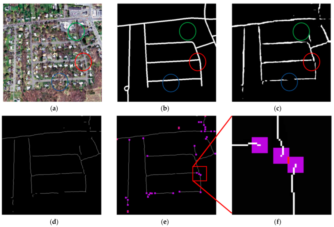
As shown in Figure 1, Figure 1a represents the input remote sensing image, Figure 1b represents the corresponding label, and Figure 1c is the segmentation result of the general semantic segmentation network and cross-entropy loss function. In Figure 1c, we found that there were many gaps in roads that should be connected. Due to the tree cover, the segmentation network classified the pixels that should have been roads as non-roads due to the visual interference of the trees, as shown in the blue circle of Figure 1c. Additionally, since most of the pixels comprising roads form linear shapes, the segmentation network was trained to judge only linear pixel shapes as roads; therefore, the road intersection shown in the red circle of Figure 1c was ignored, as it was not linearly shaped. Furthermore, we could not directly predict a more accurate image using topological algorithms to eliminate these gaps since, in reality, roads are disconnected sometimes, as shown in the green circle of Figure 1c.
The reason why a linear road may be disposed to being disconnected is due to only a few misjudged pixels needed to indicate a break in road continuity; 10 pixels, or sometimes even less, can indicate a break, depending on the road width and the ground resolution of the image. As the misjudged pixels account for an insignificant portion of the whole image, the general segmentation model and loss function cannot sufficiently capture its features in training. However, the weight of these gap pixels in the loss function can be increased to make the network pay more attention to these misjudged pixels. If these pixels are indeed errors, they are then corrected during the training of deep-learning network and decrease the loss function value, which can improve the connectivity and accuracy of road prediction.
In order to improve the proportion of these misjudged pixels that can lead to the disconnection of the predicted road in cross-entropy, these pixels must first be identified. In addition, the calculation method cannot be overly complex, as that would increase the training time and require more GPU memory, which makes it difficult, if not impossible, to complete on computers running older hardware similar to those often found in academic research environments.
A way to identify the gap pixels that cause road disconnection is to use the endpoints of road segments. Therefore, we extracted the vector line of the prediction road, as shown in Figure 1d. Next, we determined the endpoint pixels of each line and added a buffer range where the network should pay more attention, as shown in Figure 1e. The purple pixels indicate where the weight would be increased. The red pixels indicate where the two endpoints overlapped, and their weight would be doubled, as shown in the magnified image in Figure 1f. These red pixels were farther from the predicted road than the purple pixels and were, thus, prone to be misjudged more easily, so they needed doubled weight to overcome the error.
The algorithm steps of GapLoss were as follows:
- (1)
- Firstly, the predicted values of all the pixels were processed using the softmax function to acquire cross-entropy map L; then, the predicted values were binarized to acquire image A:where yi′ is the prediction value of the pixel i after the softmax function.
- (2)
- (3)
- Considering each pixel in image B, if there was only one pixel with a value of 1 in the 8 neighboring pixels, then that pixel was the endpoint, the value was set as 1, the other pixel values were set to 0, and the image was named C.
- (4)
- Considering each pixel in image C, if there was one endpoint in the neighborhood of 9 × 9 pixels, the weight of the pixel was set as K; if there were two, the weight was 2K; if there were three, the weight was 3K, and so on. If there was no endpoint in the neighborhood of 9 × 9 pixels, the weight of the pixel was set as 1. Therefore, we acquired weight map W.
- (5)
- Each pixel in weight map W was multiplied by the corresponding cross-entropy map L, and the average was calculated to acquire the GapLoss:where L is the cross-entropy map, F is the mean function, and W is the weight map.
The pseudo code of GapLoss is shown in Algorithm 1.
| Algorithm 1: GapLoss |
| Input: prediction of remote image by network |
| Output: loss function value of GapLoss |
| 1: Input is processed by softmax function to acquire cross-entropy map L |
| 2: Input is binarized to acquire image A |
| 3: Skeleton image B is obtained from A |
| 4: Generate a zeros matrix C with the same size of B |
| 5: for pixel in B |
| 6: if There is only one pixel with value of 1 in the 8 neighboring pixels, pixel is endpoint |
| 7: The corresponding pixel in C is set to 1 |
| 8: end if |
| 9: end for |
| 10: Generate a ones matrix W with the same size of B |
| 11: for pixel in C |
| 12: Obtain sum of pixel values in the 9 × 9 neighborhood as N, N is the number of endpoints in the neighborhood buffer |
| 13: If not N==0 then |
| 14: Set the corresponding pixel in W to K × N, K is a super parameter |
| 15: end if |
| 16: end for |
| 17: return the mean of W × L |
3. Experiment and Results
3.1. Evaluation Metrics
In order to objectively verify our method, we used three evaluation metrics, including the mean intersection-over-union (mIoU), Accuracy, and the F1 score for comparison and analysis.
The equation for mIoU was:
The equation for Accuracy was:
The equation for the F1 score was:
where Precision and Recall were:
where N is the number of the foreground class plus the background, and the total class number is N + 1. In this study, N was taken as 1. TP refers to a true positive, and r is the number of foreground pixels predicted as foreground correctly. FP is a false positive, which indicates the number of background pixels erroneously predicted as foreground. TN is a true negative, which indicates the number of background pixels correctly predicted as background. FN is a false negative, which indicates the number of foreground pixels erroneously predicted as background. Equation (3) used the background and road as positive samples to calculate the evaluation index and then used the average value to obtain the mIoU. The positive samples in Equations (4)–(7) were roads.
3.2. Hardware and Software
The hardware configuration of this experiment was as follows: the CPU model was Intel i5-9400F, the memory was 16 gb, the model of the graphics card was NVIDIA GeForce RTX 2060 super 8 gb, and the CUDA library version was 10.0.
Estimator, which is the official library of TensorFlow, was employed as a deep-learning framework to save on coding work. The Adam Optimizer [49] algorithm was used to find the optimal solution, and we set the learning rate at 0.0001, which was assigned as the optimal value in previous research. In addition, in order to overcome fitting issues, L2 regularization was used in the loss function, so the total loss included GapLoss and L2, as shown in Equation (8):
The test dataset was evaluated per epoch. If the metrics no longer increased for 10 periods consecutively or the max epoch number was over 100, the model training stopped immediately.
3.3. Results and Discussion of Massachusetts Roads Dataset
The evaluation metric results of the four main segmentation networks for the test set of the Massachusetts Roads Dataset are shown in Table 1. After using GapLoss, the evaluation metric values of the four segmentation networks all improved compared to those using cross-entropy.
SegNet and UNet++, which had lower segmentation accuracy with cross-entropy, were significantly improved after using GapLoss. UNet++ was the most improved network, with its mIoU increased by 4.2%, its accuracy increased by 0.4%, and its F1 score increased by 7.4%. SegNet also significantly improved, with its F1 score increased by 4.2% and its mIoU increased by 2%; its accuracy decreased slightly by −0.3%.
PSPNet and MUNet, which had higher segmentation accuracy with cross-entropy, were less improved after using GapLoss compared to UNet++. The mIoU of PSPNet increased by 2.6%, its accuracy increased by 0.2%, and its F1 score increased by 4.6%. The mIoU of MUNet increased by 2.1%, its accuracy increased by 0.5%, and its F1 score increased by 3.2%.
Moreover, based on the results of UNet++, choosing a better loss function made a segmentation network with lower segmentation accuracy become a network model with better segmentation accuracy, which further confirmed that the segmentation results were affected by both the segmentation model and the loss function and affirmed the importance of loss function research.
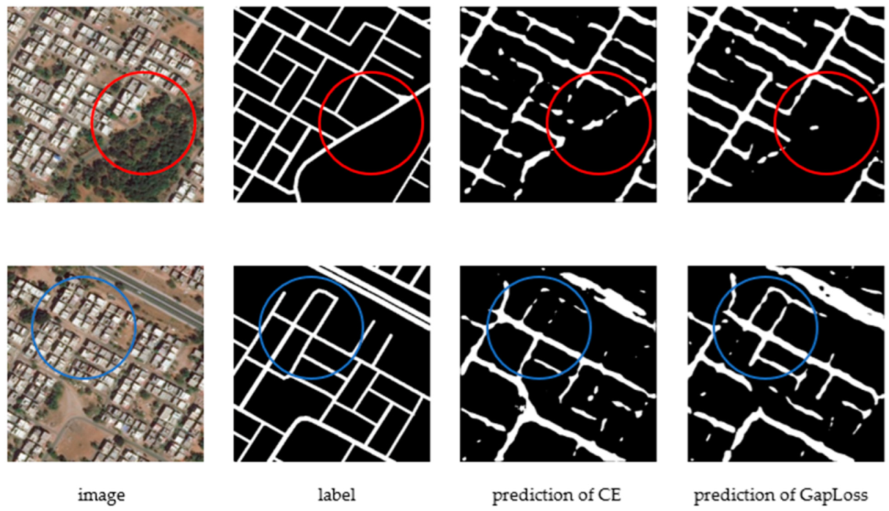
As can be seen from the prediction images of the four segmentation networks for the test dataset, the prediction results using GapLoss were improved compared to cross-entropy. As shown in the circle in Figure 2, Figure 3, Figure 4 and Figure 5, the prediction images using GapLoss showed more continuous road, and road disconnection was significantly improved. In the middle of the road, due to vehicles or trees covering the road in the remote sensing images, the predicted roads using the cross-entropy loss function had less road connection accuracy compared to the improvements using GapLoss.
At the same time, the focus of each network was different, and network with the best segmentation accuracy may not have had the most accurate connectivity, regardless of the loss function used, because the feature capture architecture of these networks was designed to focus more on reducing the probability of pixel misclassification than the topology of roads. For example, whether using cross-entropy or GapLoss, the evaluation metrics of MUNet were better than those of PSPNet, but the connectivity of the prediction image of PSPNet was better than that of MUNet.
3.4. Results and Discussion of DeepGlobe Roads Dataset
In order to that verify our conclusion that GapLoss made roads more continuous and have higher accuracy was not only applicable to the Massachusetts Roads Dataset but was also applicable to other datasets, we also compared these network models using the DeepGlobe Dataset. The evaluation metric results of the test set for the DeepGlobe Dataset are shown in Table 2. After using GapLoss, the evaluation metric values of all the segmentation networks were improved compared to those using cross-entropy.
As can be seen from Table 2, the network whose evaluation metrics improved the most was MUNet. The mIoU of MUNet increased by 4.8%, its accuracy increased by 0.5%, and its F1 score increased by 8.2%. The second was UNet++, where its mIoU increased by 4.3%, its accuracy increased by 0.3%, and its F1 score increased by 8%. The third was PSPNet, where its mIoU increased by 2.8%, its accuracy increased by 0.3%, and its F1 score increased by 4.9%. The last was SegNet, where its F1 score increased by 2.9%, and its mIoU increased by 1.5%, but its accuracy decreased by 0.1%.
These results differed from those found for the Massachusetts Roads Dataset, in which UNet++ was the most improved network. For the DeepGlobe Dataset, MUNet was the most improved network, but UNet++ was also the second-most improved, and the improved value was no less than that of the Massachusetts Roads Dataset.
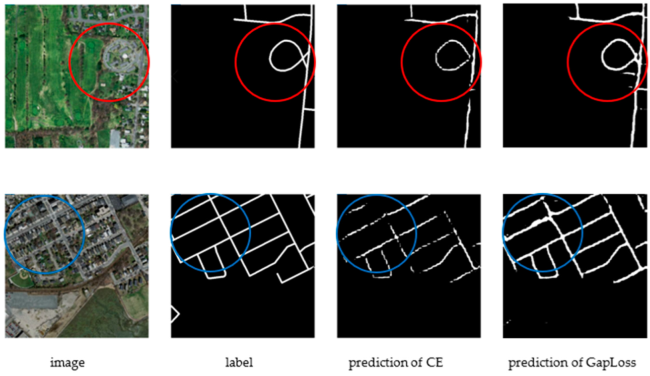
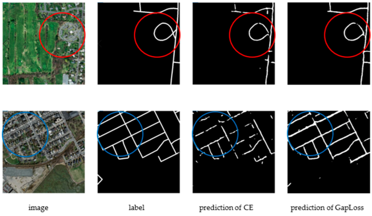
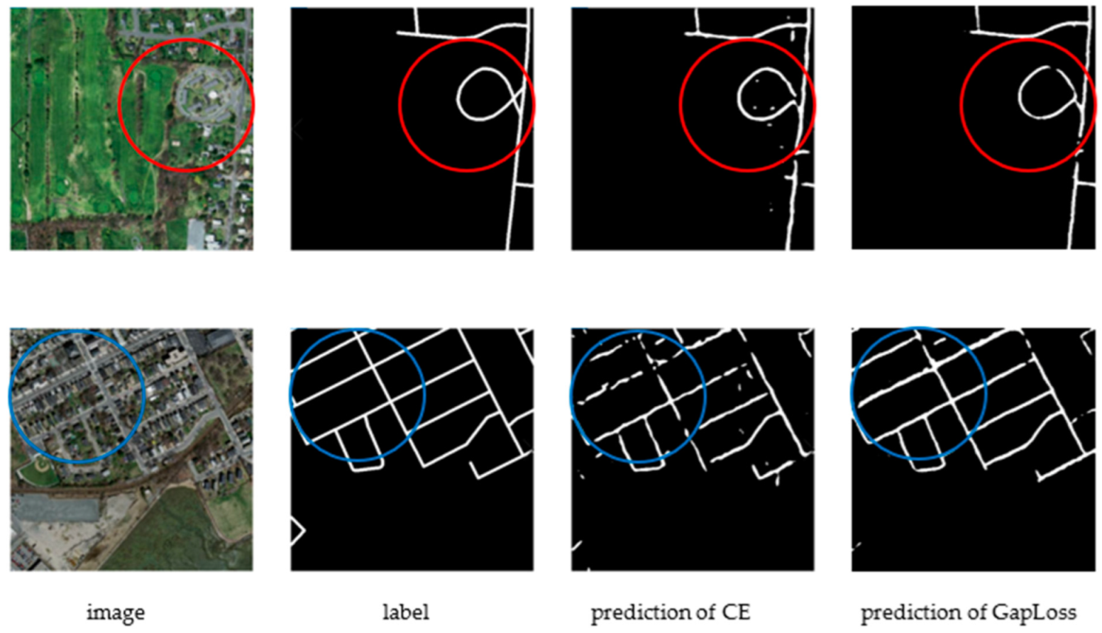
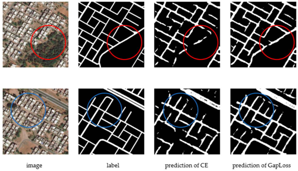
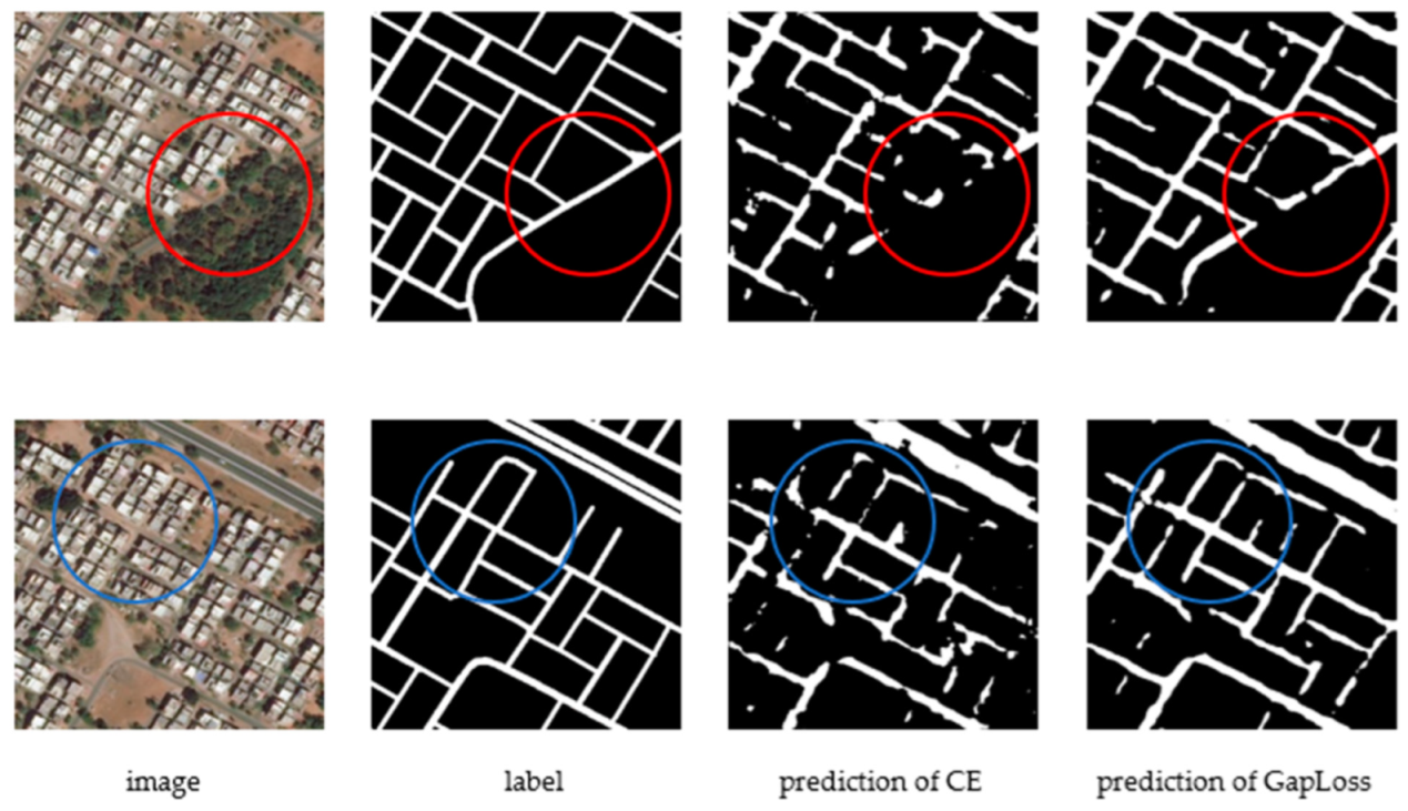
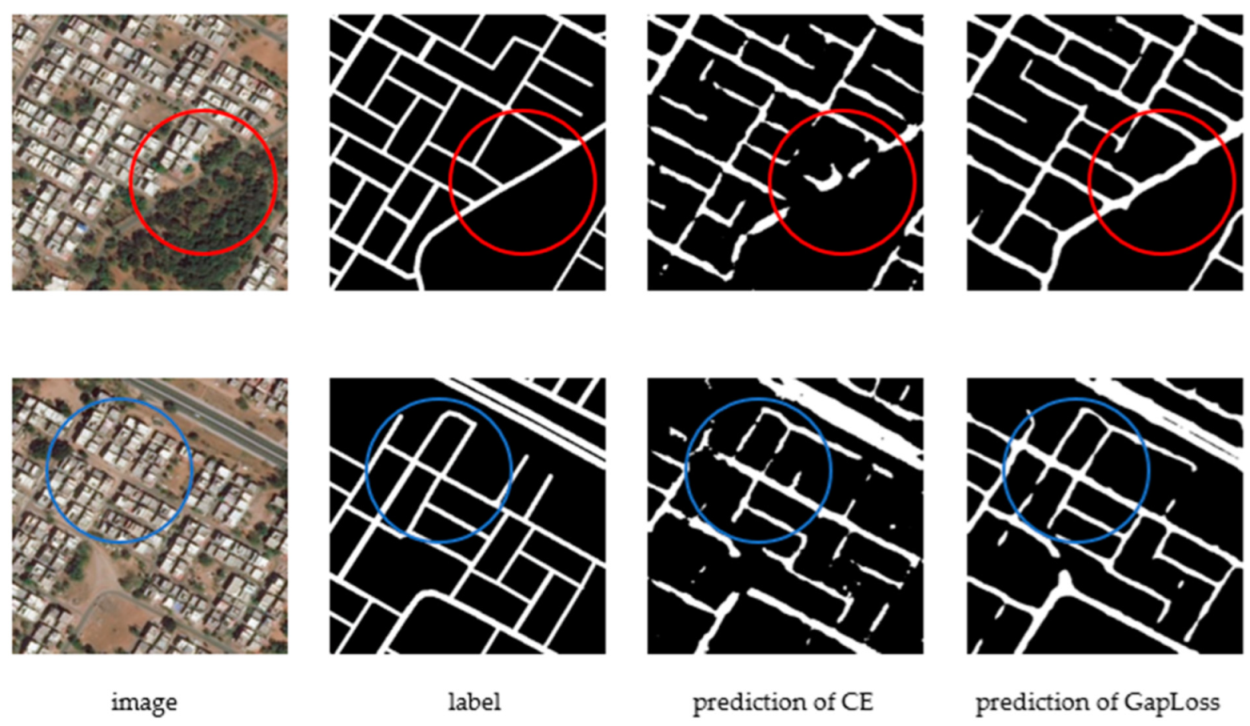
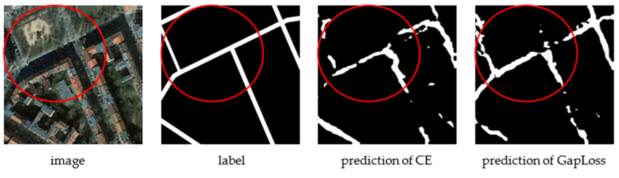
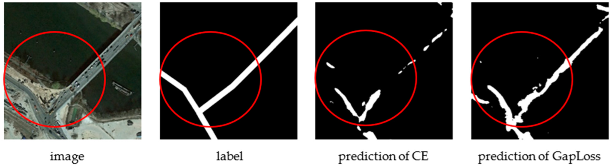
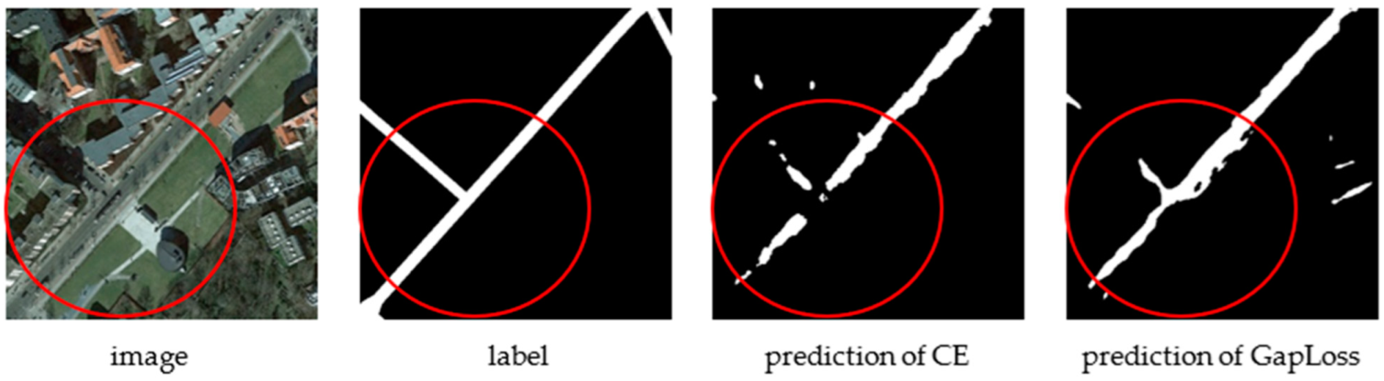
As evidenced by the prediction images of the four segmentation networks for the test dataset, although road continuity was different in the prediction images for the different segmentation networks, the prediction results using GapLoss were better than those found using cross-entropy. As shown in Figure 6, Figure 7, Figure 8 and Figure 9, the prediction images using GapLoss had improved road continuity. Intersections were better-recognized, as indicated in the blue circle in Figure 6, Figure 7, Figure 8 and Figure 9. In the middle of the road, due to possible vehicles or trees covering the road in the remote sensing images, the predicted road using cross-entropy was disconnected, whereas GapLoss accurately connected the road, as shown in the red circle in Figure 6, Figure 7, Figure 8 and Figure 9.
The road continuity predicted by the MUNet network was the best one among the four networks for the DeepGlobe Dataset. As shown in the red circle in the first row of Figure 9, the prediction results of GapLoss were barely affected by trees covering the road. The second-best was PSPNet, which ranked second in accuracy after using GapLoss, where the continuity of road intersections in the prediction image was significantly improved after using GapLoss, as shown in the blue circle in the second row of Figure 7. SegNet was the network with the worst continuity improvement among the four networks, which was consistent with the rankings of the evaluation metrics.
3.5. Results and Discussion of Aerial Image Segmentation Dataset
We also compared these network models with the Aerial Image Segmentation Dataset. The evaluation metric results of the test set for the Aerial Image Segmentation Dataset are shown in Table 3. After using GapLoss, the evaluation metric values of the all the segmentation networks were improved compared to those using cross-entropy. At the same time, we saw that the improvement was less than that of the first two datasets. This is because the ground resolution of the image in this dataset was higher, so the roads were more sparse, and the characteristics of mesh and linearity were not obvious, which led to inaccurate endpoints when calculating with GapLoss.
However, as can be seen from Table 3, the network whose evaluation metrics improved the most was PSPNet. The mIoU of PSPNet increased by 2.1%, its accuracy increased by 0.4%, and its F1 score increased by 3.3%. The second was MUNet, where its mIoU increased by 1.3%, its accuracy increased by 0.3%, and its F1 score increased by 2.2%. The third was UNet++, where its mIoU increased by 1.0%, and its F1 score increased by 1.7%. The last was SegNet, where its mIoU increased by 1.0%, its accuracy increased by 0.4%, and its F1 score increased by 1.4%.
As can be seen from the circle in Figure 10, Figure 11, Figure 12 and Figure 13, as mentioned before, the ground resolution of this dataset was higher, and the road was wider. Therefore, it could be inaccurate in calculating the endpoint of GapLoss, and the buffer may not cover all the road pixels that are obscured by trees or misjudged. However, the prediction results of GapLoss were still improved, and the road continuity was better than that of cross-entropy.
3.6. Comparison of Different K
There was a hyperparameter K found when using GapLoss. In order to verify the influence of its value on the results and to find the optimal value of K, we used the PSPNet network model as an example, which was considered the best network and is well-known, and we conducted experiments on the Massachusetts Roads Dataset from K = 0 to K = 100 at intervals of 10. The results are shown in Table 4.
As shown in Table 4, with the increase of the K value from 10, the evaluation metrics also improved until reaching K = 60. After this point, there were no further drastic changes in the evaluation accuracy beyond K = 60. This was because, when the K value was relatively small, increasing the K value effectively increased the proportion of the road gap and the intersection in the loss function of the whole image so that the network could better capture the features of these error-prone places and ensure the predicted road was accurately continuous with improved evaluation metrics. However, once the K value reached an optimal number, further increases pushed the proportion of the road gap and intersection in the loss function of the whole image too high, resulting in a decline in the network feature-capture abilities for other pixels, resulting in segmentation errors of other pixels and causing the evaluation metrics to decrease slightly.
However, no matter how the K value changed, the evaluation metrics of GapLoss were better compared to those of cross-entropy. In order to achieve the best performance, the K value of all GapLoss calculations in this study was set as 60.
3.7. Comparison of Different Loss Functions
The loss functions proposed by Batra et al. [43] and Mosinska et al. [44] were integrated with their network models and could not be combined with other network models. The loss function proposed by Xiaoling Hu [45] could not run on a computer with older hardware due to its resource-demanding calculations, and in the early stage of training, the lack of data meant the model could not calculate the topological loss function values, so it could only be used to fine-tune the training results of other loss functions. Therefore, we selected the most widely used loss functions of focal loss and dice loss for comparison to cross-entropy. Similarly, PSPNet, which is considered the best network, was selected for experimentation with the Massachusetts Roads Dataset. The results are shown in Table 5.
The mIoU of focal loss was only 68.6, while the mIoU of dice loss was only 70.6, which were not better than those of cross-entropy, but the mIoU of GapLoss was as high as 73.8, which was the best. This was due to both focal loss and dice loss being designed for unbalanced datasets. If the roads were dense in the image, the roles of focal loss and dice loss were confused and resulted in a decline in segmentation accuracy, as focal loss would ignore other road pixels in favor of pixels that were difficult to classify.
3.8. Pseudo-Error
As can be seen in Figure 2, Figure 3, Figure 4, Figure 5, Figure 6, Figure 7, Figure 8, Figure 9, Figure 10, Figure 11, Figure 12 and Figure 13, after using GapLoss, the road connectivity was significantly improved, not only at the intersection but also in the middle of the road. Theoretically, as roads account for less in an overall image, once the road connectivity is improved, the proportion of correctly predicted pixels of the total roads should increase, and the evaluation metrics should increase significantly. However, the experimental results indicated that the evaluation metrics did not increase as much as we had anticipated. This was attributed to the labeling accuracy of the Massachusetts Roads Dataset being low. Some roads were not labeled due to manual error based on the predefined knowledge of the annotator. We referred to these faults as “pseudo-errors” (i.e., the actual predictions were correct but, as they were not labeled, they were considered as errors when calculating the evaluation metrics).
As shown in the red circle of the first and third rows of the remote sensing images in Figure 14, there was a road between the main road and the house, but it was not annotated in the label. The prediction result of the cross-entropy loss function found the path, but it was not connected with the main road, so there were a few false error pixels. However, in the prediction results of GapLoss, the path was complete, so there were more false errors. The second row in Figure 14 shows a more obvious example where many roads in the red circle were not marked in the label. The annotator may have thought that it was an internal road and should not be marked, but this is a subjective judgment. For a computer, these pixels definitely indicate a road, and they make up a large proportion of this image and will impact the evaluation metrics. Therefore, after using GapLoss, although the connectivity of the road was improved and the prediction accuracy was improved, the false errors also increased, which lowered the accuracy. The final accuracy increase was not as evident as what was observed in the images.
4. Conclusions and Future Work
In this work, a loss function called GapLoss was proposed to solve the discontinuity issues in roads extracted from remote sensing images by deep-learning networks. GapLoss can be chosen independently from the segmentation network model chosen, as it can be combined with any existing or future segmentation network model, so the best choice for each can be chosen based on the proposed task. Experiments on four main segmentation networks were performed using the Massachusetts Roads Dataset and the DeepGlobe dataset using both cross-entropy and GapLoss. The results indicated that GapLoss greatly improved the road connectivity, especially at intersections and when the view of the road was obscured by trees or other structures. The road prediction by the segmentation networks with GapLoss was also more continuous.
Based on the evaluation metrics, after using GapLoss, nearly all the evaluation metrics of the four segmentation networks were improved. GapLoss not only improved the connectivity of the predicted road, but also simultaneously improved the accuracy of road prediction at the same time, which topological loss has not been able to achieve. Therefore, GapLoss as proposed in this paper has the potential to play a significant role in the semantic segmentation of roads in remote sensing images.
In this experiment, we used only three bands for image segmentation. In future research, we will examine the role of multispectral bands in remote sensing image road segmentation. GapLoss is applicable when roads are mesh or linear. If the ground resolution of the image is too high, the roads are wide and it is inaccurate in calculating the endpoint of GapLoss. In this case, the buffer may not cover all the road pixels that are obscured by trees or misjudged, and the improvement from GapLoss will not be obvious.
Author Contributions
W.Y. got fund, designed the comparative experiments, coded and wrote the manuscript; W.X. supervised the study and revised the manuscript. All authors have read and agreed to the published version of the manuscript.
Funding
This research was funded by the open fund of the Key Laboratory of Pattern Recognition and Intelligent Information Processing, Institutions of Higher Education of Sichuan Province, Chengdu University (MSSB-2021-04).
Data Availability Statement
The data used in this study are open datasets. The datasets can be downloaded from https://www.cs.toronto.edu/~vmnih/data/ (accessed on 5 June 2021).
Acknowledgments
We would like to thank the anonymous reviewers for their constructive and valuable suggestions on earlier drafts of this manuscript.
Conflicts of Interest
The authors declare that there is no conflict of interest.
References
- Laptev, I.; Mayer, H.; Lindeberg, T.; Eckstein, W.; Steger, C.; Baumgartner, A. Automatic Extraction of Roads from Aerial Images Based on Scale Space and Snakes. Mach. Vis. Appl. 2000, 12, 23–31. [Google Scholar] [CrossRef] [Green Version]
- Maboudi, M.; Amini, J.; Hahn, M.; Saati, M. Object-based road extraction from satellite images using ant colony optimization. Int. J. Remote Sens. 2017, 38, 179–198. [Google Scholar] [CrossRef]
- Wu, X.W.; Xu, H.Q. Level set method major roads information extract from high-resolution remote-sensing imagery. J. Astronaut. 2010, 31, 1495–1502. [Google Scholar]
- Cai, H.; Yao, G. Optimized method for road extraction from high resolution remote sensing image based on watershed algorithm. Remote Sens. Land Resour. 2013, 25, 25–29. [Google Scholar]
- Breiman, L. Random forests. Mach. Learn. 2001, 45, 5–32. [Google Scholar] [CrossRef] [Green Version]
- Vapnik, V.; Chervonenkis, A. A note on class of perceptron. Autom. Remote Control 1964, 24, 112–120. [Google Scholar]
- Tupin, F.; Maitre, H.; Mangin, J.; Nicolas, J.; Pechersky, E. Detection of linear features in SAR images: Application to road network extraction. IEEE Trans. Geosci. Remote Sens. 1998, 36, 434–453. [Google Scholar] [CrossRef] [Green Version]
- Li, Y.; Zhang, R.; Wu, Y. Road network extraction in high-resolution SAR images based CNN features. In Proceedings of the 2017 IEEE International Geoscience and Remote Sensing Symposium (IGARSS), Fort Worth, TX, USA, 23–28 July 2017; pp. 1664–1667. [Google Scholar]
- Zhu, D.; Wen, X.; Ling, C. Road extraction based on the algorithms of MRF and hybrid model of SVM and FCM. In Proceedings of the 2011 International Symposium on Image and Data Fusion, Tengchong, China, 9–11 August 2011; pp. 1–4. [Google Scholar]
- Miao, Z.; Wang, B.; Shi, W.; Zhang, H. A semi-automatic method for road centerline extraction from VHR images. IEEE Geosci. Remote Sens. Lett. 2014, 11, 1856–1860. [Google Scholar] [CrossRef]
- Zhang, J.; Chen, L.; Li, Z.; Geng, W.; Wang, C. Multiple saliency features based automatic road extraction from high-resolution multispectral satellite images. Chin. J. Electron. 2018, 27, 133–139. [Google Scholar] [CrossRef]
- Maurya, R.; Gupta, P.R.; Shukla, A.S. Road extraction using K-means clustering and morphological operations. In Proceedings of the 2011 International Conference on Image Information Processing, Shimla, India, 3–5 November 2011; pp. 1–6. [Google Scholar]
- Ronneberger, O.; Fischer, P.; Brox, T. Convolutional networks for biomedical image segmentation. In Proceedings of the 2015 Medical Image Computing and Computer Assisted Intervention (MICCAI 2015), Piscataway, NJ, USA, 5–9 October 2015; pp. 234–241. [Google Scholar]
- Chen, L.C.; Papandreou, G.; Kokkinos, I.; Murphy, K.; Yuille, A.L. Semantic image segmentation with deep convolutional nets and fully connected crfs. arXiv 2014, arXiv:1412.7062. [Google Scholar]
- Chen, L.; Papandreou, G.; Kokkinos, I.; Murphy, K.; Yuille, A.L. DeepLab: Semantic image segmentation with deep convolutional nets, atrous convolution, and fully connected crfs. IEEE Trans. Pattern Anal. Mach. Intell. 2018, 40, 834–848. [Google Scholar] [CrossRef] [PubMed] [Green Version]
- Chen, L.-C.; Papandreou, G.; Schroff, F.; Adam, H. Rethinking Atrous Convolution for Semantic Image Segmentation. arXiv 2017, arXiv:1706.05587. [Google Scholar]
- Chen, L.C.; Zhu, Y.; Papandreou, G.; Schroff, F.; Adam, H. Encoder-decoder with atrous separable convolution for semantic image segmentation. In Proceedings of the European Conference on Computer Vision, Munich, Germany, 8–14 September 2018; pp. 833–851. [Google Scholar]
- Badrinarayanan, V.; Kendall, A.; Cipolla, R. Segnet: A deep convolutional encoder-decoder architecture for image segmentation. IEEE Trans. Pattern Anal. Mach. Intell. 2017, 39, 2481–2495. [Google Scholar] [CrossRef] [PubMed]
- Zhao, H.; Shi, J.; Qi, X.; Wang, X.; Jia, J. Pyramid scene parsing network. In Proceedings of the 2017 IEEE Conference on Computer Vision and Pattern Recognition (CVPR), Honolulu, HI, USA, 21–26 July 2017; pp. 6230–6239. [Google Scholar] [CrossRef] [Green Version]
- Zhou, Z.; Siddiquee, M.M.R.; Tajbakhsh, N.; Liang, J. UNet++: Redesigning skip connections to exploit multiscale features in image segmentation. IEEE Trans. Med. Imaging 2020, 39, 1856–1867. [Google Scholar] [CrossRef] [PubMed] [Green Version]
- Yuan, W.; Zhou, T.; Xi, Z.S.; Zhou, X.Y. MUNet: A multi-branch adaptive deep learning network for remote sensing image semantic segmentation. J. Geomat. Sci. Technol. 2020, 37, 581–588. (In Chinese) [Google Scholar]
- Zhong, Z.; Li, J.; Cui, W.; Jiang, H. Fully convolutional networks for building and road extraction: Preliminary results. In Proceedings of the 2016 IEEE International Geoscience and Remote Sensing Symposium (IGARSS), Beijing, China, 10–15 July 2016; pp. 1591–1594. [Google Scholar] [CrossRef]
- Mnih, V. Machine Learning for Aerial Image Labeling; Department of Computer Science, University of Toronto: Toronto, ON, Canada, 2013. [Google Scholar]
- Panboonyuen, T.; Vateekul, P.; Jitkajornwanich, K.; Lawawirojwong, S. An enhanced deep convolutional encoder-decoder network for road segmentation on aerial imagery. In Advances in Intelligent Systems and Computing: Proceedings of the International Conference on Computing& Information Technology; Springer: Kusadasi, Turkey, 2017; pp. 191–201. [Google Scholar]
- Wei, Y.; Wang, Z.; Xu, M. Road Structure Refined CNN for Road Extraction in Aerial Image. IEEE Geosci. Remote Sens. Lett. 2017, 14, 709–713. [Google Scholar] [CrossRef]
- Máttyus, G.; Luo, W.; Urtasun, R. DeepRoadMapper: Extracting Road Topology from Aerial Images. In Proceedings of the 2017 IEEE International Conference on Computer Vision (ICCV), Venice, Italy, 22–29 October 2017; pp. 3458–3466. [Google Scholar] [CrossRef]
- Gao, X.; Sun, X.; Zhang, Y.; Yan, M.; Xu, G.; Sun, H.; Jiao, J.; Fu, K. An End-to-End Neural Network for Road Extraction from Remote Sensing Imagery by Multiple Feature Pyramid Network. IEEE Access 2018, 6, 39401–39414. [Google Scholar] [CrossRef]
- Zhang, Z.; Liu, Q.; Wang, Y. Road extraction by deep residual U-Net. IEEE Geosci. Remote Sens. Lett. 2018, 15, 749–753. [Google Scholar] [CrossRef] [Green Version]
- Xu, Y.; Xie, Z.; Feng, Y.; Chen, Z. Road extraction from high resolution remote sensing imagery using deep learning. Remote Sens. 2018, 10, 1461. [Google Scholar] [CrossRef] [Green Version]
- Zhou, L.; Zhang, C.; Wu, M. D-Linknet: LinkNet with pretrained encoder and dilated convolution for high resolution satellite imagery road extraction. In Proceedings of the IEEE Conference on Computer Vision and Pattern Recognition Workshops, Salt Lake City, UT, USA, 18–22 June 2018; pp. 192–196. [Google Scholar]
- DeepGlobe. 2018. Available online: http://deepglobe.org/ (accessed on 10 June 2021).
- Buslaev, A.; Seferbekov, S.; Iglovikov, V.; Shvets, A. Fully convolutional network for automatic road extraction from satellite imagery. In Proceedings of the IEEE Conference on Computer Vision and Pattern Recognition Workshops, Salt Lake City, UT, USA, 18–22 June 2018; pp. 197–200. [Google Scholar]
- Bonafilia, D.; Gill, J.; Basu, S.; Yang, D. Building high resolution maps for humanitarian aid and development with weakly-and semi-supervised learning. In Proceedings of the IEEE/CVF Conference on Computer Vision and Pattern Recognition Workshops, Long Beach, CA, USA, 16–20 June 2019; pp. 1–9. [Google Scholar]
- Wu, S.; Du, C.; Chen, H.; Xu, Y.; Guo, N.; Jing, N. Road extraction from very high resolution images using weakly labeled OpenStreetMap centerline. ISPRS Int. J. Geo-Inf. 2019, 8, 478. [Google Scholar] [CrossRef] [Green Version]
- Wang, S.; Yang, H.; Wu, Q.; Zheng, Z.; Wu, Y.; Li, J. An improved method for road extraction from highresolution remote-sensing images that enhances boundary information. Sensors 2020, 20, 2064. [Google Scholar] [CrossRef] [PubMed] [Green Version]
- Yuan, W.; Xu, W. NeighborLoss: A Loss Function Considering Spatial Correlation for Semantic Segmentation of Remote Sensing Image. IEEE Access 2021, 9, 75641–75649. [Google Scholar] [CrossRef]
- YA, D.M.; Liu, Q.; Qian, Z.B. Automated image segmentation using improved PCNN model based on cross-entropy. In Proceedings of the 2004 International Symposium on Intelligent Multimedia, Video and Speech Processing, Hong Kong, China, 20–22 October 2004; pp. 743–746. [Google Scholar] [CrossRef]
- Lin, T.; Goyal, P.; Girshick, R.; He, K.; Dollár, P. Focal loss for dense object detection. IEEE Trans. Pattern Anal. Mach. Intell. 2020, 42, 318–327. [Google Scholar] [CrossRef] [Green Version]
- Milletari, F.; Navab, N.; Ahmadi, S. V-Net: Fully convolutional neural networks for volumetric medical image segmentation. In Proceedings of the 2016 Fourth International Conference on 3D Vision (3DV), Stanford, CA, USA, 25–28 October 2016; pp. 565–571. [Google Scholar] [CrossRef] [Green Version]
- Salehi, S.; Erdogmus, D.; Gholipour, A. Tversky loss function for image segmentation using 3d fully convolutional deep networks. In Proceedings of the International Workshop on Machine Learning in Medical Imaging, Quebec, QC, Canada, 10 September 2017; pp. 379–387. [Google Scholar]
- Jadon, S. A survey of loss functions for semantic segmentation. In Proceedings of the 2020 IEEE Conference on Computational Intelligence in Bioinformatics and Computational Biology (CIBCB), Via del Mar, Chile, 27–29 October 2020; pp. 1–7. [Google Scholar] [CrossRef]
- Crum, W.R.; Camara, O.; Hill, D.L.G. Generalized overlap measures for evaluation and validation in medical image analysis. IEEE Trans. Med. Imaging 2006, 25, 1451–1461. [Google Scholar] [CrossRef]
- Batra, A.; Singh, S.; Pang, G.; Basu, S.; Jawahar, C.V.; Paluri, M. Improved Road Connectivity by Joint Learning of Orientation and Segmentation. In Proceedings of the 2019 IEEE/CVF Conference on Computer Vision and Pattern Recognition (CVPR), Long Beach, CA, USA, 15–20 June 2019; pp. 10377–10385. [Google Scholar] [CrossRef]
- Mosinska, A.; Marquez-Neila, P.; Koziński, M.; Fua, P. Beyond the pixel-wise loss for topology-aware delineation. In Proceedings of the IEEE Conference on Computer Vision and Pattern Recognition, Salt Lake City, UT, USA, 18–22 June 2018; pp. 3136–3145. [Google Scholar]
- Hu, X.; Li, F.; Samaras, D.; Chen, C. Topology-Preserving Deep Image Segmentation. arXiv 2019, arXiv:1906.05404. [Google Scholar]
- Lashgari, E.; Liang, D.; Maoz, U. Data augmentation for deep learning-based electroencephalography. J. Neurosci. Methods 2020, 346, 108885. [Google Scholar] [CrossRef]
- Liu, W.; Zhang, C.; Lin, G.; Liu, F. CRNet: Cross-reference networks for few-shot segmentation. In Proceedings of the 2020 IEEE/CVF Conference on Computer Vision and Pattern Recognition (CVPR), Seattle, WA, USA, 13–19 June 2020; pp. 4164–4172. [Google Scholar] [CrossRef]
- Kaiser, P.; Wegner, J.D.; Lucchi, A.; Jaggi, M.; Hofmann, T.; Schindler, K. Learning Aerial Image Segmentation from Online Maps. IEEE Trans. Geosci. Remote Sens. 2017, 55, 6054–6068. [Google Scholar] [CrossRef]
- Kingma, D.P.; Ba, J. Adam: A method for stochastic optimization. In Proceedings of the 3rd International Conference for Learning Representations, San Diego, CA, USA, 7–9 May 2015; pp. 1–15. [Google Scholar]
Figure 1.
Calculation diagram of GapLoss. (a) Input remote sensing image, (b) corresponding label, (c) predicted road by deep-learning network, (d) skeleton of predicted road, (e) weight map by buffering of endpoint, and (f) a partial enlarged view of (e). In (a–c), the blue circle is the road covered by trees, the red circle is the road intersection, and the green circle is the unconnected road. The red square of (e) is the range of figure (f) in figure (e). The purple pixels in (e,f) represent the buffer area generated by the end point of the road, and the red pixels represent the overlapping area of the two end point buffers.

Figure 2.
SegNet results with CE and GapLoss on Massachusetts Roads Dataset. The blue and red circles indicate where the road continuity is improved after using GapLoss.
Figure 2.
SegNet results with CE and GapLoss on Massachusetts Roads Dataset. The blue and red circles indicate where the road continuity is improved after using GapLoss.

Figure 3.
PSPNet results with CE and GapLoss on Massachusetts Roads Dataset. The blue and red circles indicate where the road continuity is improved after using GapLoss.
Figure 3.
PSPNet results with CE and GapLoss on Massachusetts Roads Dataset. The blue and red circles indicate where the road continuity is improved after using GapLoss.

Figure 4.
UNet++ results with CE and GapLoss on Massachusetts Roads Dataset. The blue and red circles indicate where the road continuity is improved after using GapLoss.
Figure 4.
UNet++ results with CE and GapLoss on Massachusetts Roads Dataset. The blue and red circles indicate where the road continuity is improved after using GapLoss.

Figure 5.
MUNet results with CE and GapLoss on Massachusetts Roads Dataset. The blue and red circles indicate where the road continuity is improved after using GapLoss.
Figure 5.
MUNet results with CE and GapLoss on Massachusetts Roads Dataset. The blue and red circles indicate where the road continuity is improved after using GapLoss.

Figure 6.
SegNet results with CE and GapLoss on DeepGlobe Roads Dataset. The blue and red circles indicate where the road continuity is improved after using GapLoss.
Figure 6.
SegNet results with CE and GapLoss on DeepGlobe Roads Dataset. The blue and red circles indicate where the road continuity is improved after using GapLoss.

Figure 7.
PSPNet results with CE and GapLoss on DeepGlobe Roads Dataset. The blue and red circles indicate where the road continuity is improved after using GapLoss.
Figure 7.
PSPNet results with CE and GapLoss on DeepGlobe Roads Dataset. The blue and red circles indicate where the road continuity is improved after using GapLoss.

Figure 8.
UNet++ results with CE and GapLoss on DeepGlobe Roads Dataset. The blue and red circles indicate where the road continuity is improved after using GapLoss.
Figure 8.
UNet++ results with CE and GapLoss on DeepGlobe Roads Dataset. The blue and red circles indicate where the road continuity is improved after using GapLoss.

Figure 9.
MUNet results with CE and GapLoss on DeepGlobe Roads Dataset. The blue and red circles indicate where the road continuity is improved after using GapLoss.
Figure 9.
MUNet results with CE and GapLoss on DeepGlobe Roads Dataset. The blue and red circles indicate where the road continuity is improved after using GapLoss.

Figure 10.
SegNet results with CE and GapLoss on Aerial Image Segmentation Dataset.

Figure 11.
PSPNet results with CE and GapLoss on Aerial Image Segmentation Dataset.

Figure 12.
Unet++ results with CE and GapLoss on Aerial Image Segmentation Dataset.

Figure 13.
MUNet results with CE and GapLoss on Aerial Image Segmentation Dataset.

Figure 14.
Some controversial misjudgments.


Table 1.
The results of Massachusetts Roads Dataset.
| Methods | mIoU | Accuracy | F1 Score |
|---|---|---|---|
| SegNet and Cross-Entropy | 69.6 | 96.7 | 59.6 |
| SegNet and GapLoss | 71.6 | 96.4 | 63.8 |
| UNet++ and Cross-Entropy | 70.4 | 96.7 | 61.2 |
| UNet++ and GapLoss | 74.6 | 97.1 | 68.6 |
| PSPNet and Cross-Entropy | 71.2 | 96.7 | 62.8 |
| PSPNet and GapLoss | 73.8 | 96.9 | 67.4 |
| MUNet and Cross-Entropy | 71.9 | 96.7 | 64.2 |
| MUNet and GapLoss | 74.0 | 97.2 | 67.4 |
Table 2.
The results of DeepGlobe Roads Dataset.
| Methods | mIoU | Accuracy | F1 Score |
|---|---|---|---|
| SegNet and Cross-Entropy | 68.8 | 97.1 | 57.8 |
| SegNet and GapLoss | 70.3 | 97.0 | 60.7 |
| UNet++ and Cross-Entropy | 68.2 | 96.9 | 56.8 |
| UNet++ and GapLoss | 72.5 | 97.2 | 64.8 |
| PSPNet and Cross-Entropy | 71.6 | 97.1 | 63.1 |
| PSPNet and GapLoss | 74.4 | 97.4 | 68.0 |
| MUNet and Cross-Entropy | 71.1 | 97.1 | 62.2 |
| MUNet and GapLoss | 75.9 | 97.6 | 70.4 |
Table 3.
The results of SegNet and UNet++ on Aerial Image Segmentation Dataset.
| Methods | mIoU | Accuracy | F1 Score |
|---|---|---|---|
| SegNet and Cross-Entropy | 71.0 | 92.1 | 67.2 |
| SegNet and GapLoss | 72.0 | 92.5 | 68.6 |
| UNet++ and Cross-Entropy | 70.5 | 92.1 | 66.3 |
| UNet++ and GapLoss | 71.5 | 92.1 | 68.0 |
| PSPNet and Cross-Entropy | 70.3 | 91.8 | 66.2 |
| PSPNet and GapLoss | 72.4 | 92.2 | 69.5 |
| MUNet and Cross-Entropy | 71.0 | 92.4 | 66.7 |
| MUNet and GapLoss | 72.3 | 92.7 | 68.9 |
Table 4.
The results of PSPNet with different K values on Massachusetts Roads Dataset.
| K | mIoU | Accuracy | F1 Score |
|---|---|---|---|
| 10 | 72.7 | 96.9 | 65.4 |
| 20 | 72.7 | 96.9 | 65.4 |
| 30 | 73.3 | 96.9 | 66.5 |
| 40 | 73.8 | 97.0 | 67.2 |
| 50 | 73.6 | 97.0 | 67.0 |
| 60 | 73.8 | 96.9 | 67.4 |
| 70 | 73.4 | 97.0 | 66.6 |
| 80 | 73.5 | 96.9 | 66.9 |
| 90 | 73.4 | 97.0 | 66.7 |
| 100 | 73.4 | 97.0 | 66.7 |
Table 5.
Comparison of different loss functions on Massachusetts Roads Dataset.
| Methods | mIoU | Accuracy | F1 Score |
|---|---|---|---|
| PSPNet and Cross-Entropy | 71.2 | 96.7 | 62.8 |
| PSPNet and Focal Loss | 68.6 | 96.8 | 57.6 |
| PSPNet and Dice Loss | 70.6 | 96.4 | 62.0 |
| PSPNet and GapLoss | 73.8 | 96.9 | 65.4 |
Publisher’s Note: MDPI stays neutral with regard to jurisdictional claims in published maps and institutional affiliations. |
© 2022 by the authors. Licensee MDPI, Basel, Switzerland. This article is an open access article distributed under the terms and conditions of the Creative Commons Attribution (CC BY) license (https://creativecommons.org/licenses/by/4.0/).
Share and Cite
MDPI and ACS Style
Yuan, W.; Xu, W. GapLoss: A Loss Function for Semantic Segmentation of Roads in Remote Sensing Images. Remote Sens. 2022, 14, 2422. https://0-doi-org.brum.beds.ac.uk/10.3390/rs14102422
AMA Style
Yuan W, Xu W. GapLoss: A Loss Function for Semantic Segmentation of Roads in Remote Sensing Images. Remote Sensing. 2022; 14(10):2422. https://0-doi-org.brum.beds.ac.uk/10.3390/rs14102422
Chicago/Turabian StyleYuan, Wei, and Wenbo Xu. 2022. "GapLoss: A Loss Function for Semantic Segmentation of Roads in Remote Sensing Images" Remote Sensing 14, no. 10: 2422. https://0-doi-org.brum.beds.ac.uk/10.3390/rs14102422
Note that from the first issue of 2016, this journal uses article numbers instead of page numbers. See further details here.