
TE-SAGAN: An Improved Generative Adversarial Network for Remote Sensing Super-Resolution Images


1
School of Computer Science, China University of Geosciences, Wuhan 430074, China
2
National Engineering Research Center of Geographic Information System, China University of Geosciences, Wuhan 430074, China
3
Key Laboratory of Urban Land Resources Monitoring and Simulation, Ministry of Natural Resources, Shenzhen 518034, China
4
School of Geography and Information Engineering, China University of Geosciences, Wuhan 430074, China
*
Author to whom correspondence should be addressed.
Remote Sens. 2022, 14(10), 2425; https://doi.org/10.3390/rs14102425
Submission received: 30 March 2022
/
Revised: 13 May 2022
/
Accepted: 17 May 2022
/
Published: 18 May 2022
Abstract
:Resolution is a comprehensive reflection and evaluation index for the visual quality of remote sensing images. Super-resolution processing has been widely applied for extracting information from remote sensing images. Recently, deep learning methods have found increasing application in the super-resolution processing of remote sensing images. However, issues such as blurry object edges and existing artifacts persist. To overcome these issues, this study proposes an improved generative adversarial network with self-attention and texture enhancement (TE-SAGAN) for remote sensing super-resolution images. We first designed an improved generator based on the residual dense block with a self-attention mechanism and weight normalization. The generator gains the feature extraction capability and enhances the training model stability to improve edge contour and texture. Subsequently, a joint loss, which is a combination of L1-norm, perceptual, and texture losses, is designed to optimize the training process and remove artifacts. The L1-norm loss is designed to ensure the consistency of low-frequency pixels; perceptual loss is used to entrench medium- and high-frequency details; and texture loss provides the local features for the super-resolution process. The results of experiments using a publicly available dataset (UC Merced Land Use dataset) and our dataset show that the proposed TE-SAGAN yields clear edges and textures in the super-resolution reconstruction of remote sensing images.
1. Introduction
The development of optical remote sensing technology has enabled researchers to obtain large-area, multi-temporal Earth observation images for social construction with ease. Nevertheless, optical satellite image quality suffers from the sensor imaging technology, limiting the quality and application of remote sensing images. Low-resolution remote sensing images bring trouble to ground object interpretations. Therefore, super-resolution reconstruction of remote sensing images has become an indispensable preprocessing step. Improving the spatial resolution of remote sensing images promotes clearer object boundaries and contours in remote sensing images, which provides clear data for subsequent applications of extracting features, such as the recognition roads and buildings by semantic segmentation methods [1,2,3] or change detection by extracting the object boundary [4,5]. Therefore, the super-resolution processing of remote sensing images has become an indispensable preprocessing process. Many researchers have utilized super-resolution techniques to effectively and accurately obtain images [6,7,8,9,10]. Super-resolution (SR) imaging is a technology that uses single or multiple low-resolution (LR) images to obtain high-resolution (HR) images using existing image acquisition devices. It has been widely applied since the 1980s, and Huang et al. [11] creatively proposed a method for reconstructing HR images based on the frequency field of multi-frame sequential LR images. Since then, SR processing of remote sensing images has become an active research topic, and numerous pertinent algorithms have been designed. At present, researchers have divided single-image super-resolution (SISR) processing methods into interpolation-, reconstruction-, and learning-based methods.
The interpolation-based method estimates the unknown pixel value via interpolation in the designed linear function according to the known pixels, such as nearest-neighbor interpolation [12], Lanczos filtering [13], or bicubic filtering [14]. Although these methods can achieve rapid SR image processing, filling the pixels with low-frequency information leads to shortcomings in the overall semantic features. Consequently, the super-resolution images may lose information of some details or boundaries may not be clear. Reconstruction-based methods aim to establish an appropriate prior constraint or registration model between LR and HR images, such as projection onto convex sets [15,16,17], iterative back projection [18], or maximum a posteriori probability method [19,20,21]. The core objective of reconstruction-based methods is to build a reasonable prior observation model. However, SR imaging is a highly underdetermined infinite-solution problem in mathematical theory. Even using the optimal parameters, the transformation performance of the model is weak in diverse tasks. Owing to this problem, the model requires considerable resources to accomplish repeatable and complicated calculations.
In recent years, with the development of machine learning frameworks, academic interest in learning-based methods has increased, particularly deep learning driven by big data [22]. Convolutional neural networks are a representative adaptive learning method widely used for the reconstruction of low- and high-frequency images and are less complex than traditional manual interventions. Researchers have thus expanded and applied convolutional neural networks to SR image tasks [23,24,25,26,27,28]. However, both early shallow networks with 3–5 layers [29,30] and deep super-resolution networks [31,32,33] tend to produce low-frequency results.
To address these issues, researchers have explored algorithms that yield results consistent with human observations and sought alternatives capable of obtaining high-frequency images. Ledig et al. [34] proposed an improved generative adversarial network (GAN) model, named SRGAN, which benefits from content and perceptual losses and exerts good performance. Based on SRGAN, the Residual-in-Residual Dense Block (RRDB) was introduced, which further improved the recovered image texture [35]. In the last years, many ESRGAN-based algorithms [36,37,38] have been improved. ESRGAN+ [36] replaces ESRGAN’s RRDB with RRDRB; Real-ESRGAN replaces the VGG-Net type discriminator in the original ESRGAN with a U-Net type discriminator [37], which has a good improvement in anime images and videos. However, these network parameters are too large to fit training conditions. When these methods are used to reconstruct remote sensing images, the texture details are still unclear, and some artifacts remain in the produced images.
The primary reasons for the abovementioned problems can be summarized as follows: (1) Owing to their peculiar characteristics compared to conventional images of the same image dimensions, remote sensing images contain abundant information, such as external contours and internal textures, that characterize the spatial relationships of ground objects, thereby making the content appear crowded. Therefore, algorithms that can accurately recover and characterize contours and internal textures are necessary. (2) Most existing methods do not consider global spatial connectivity and refining texture in the algorithm design. Owing to the local perception characteristic of convolutional neural networks, global feature information in large-scale remote scenes is ignored. Thus, the global remote sensing information is neglected and underutilized.
To resolve these concerns, we present TE-SAGAN, a GAN-based texture-enhanced SR processing network for remote sensing images, which sharpens SR image details while maintaining clear visual edges. The self-attention mechanism (SAM) is designed to learn global information from remote sensing images. Furthermore, the RRDB was introduced for image depth extraction. Simultaneously, a SAM with three submodules was used to obtain different levels of attention, where relevant information (such as edge contours) can be engaged and received dynamically. Weight normalization (WN) [39] was also introduced to TE-SAGAN to remove artifacts and increase the training network stability. The calculated texture loss by the Gram matrix was designed to assess the difference between the original HR and SR images in high-frequency features, which can help improve the internal details of the reconstructed image.
In conclusion, by the self-attention module and texture loss units, this work provides insight into refining the image edges and textures. The major contributions are as follows: (1) designing the self-attention mechanism module for extracting the global information, which can decrease the limitation of the local receptive field and increase the super-resolution network accuracy; (2) a weight normalization layer is introduced instead of batch normalization, which can reduce the interference of mini-batch data on reconstructed image quality and improve the image artifact; (3) a joint loss is designed combining the content loss, perceptual loss, adversarial loss, and texture loss, which take into account the consistency of the pixel content and texture details and promote the super resolution work to achieve a characteristic remote sensing image.
2. Method
2.1. Principle of the Proposed Method
The designed network framework proposed in this study is based on GAN [40] and comprises two parts: a generator network and a discriminator network. The generator network consists of feed-forward neural networks to form the feature extraction module, which is expressed by the function , where denotes the weights and biases of the neural network layer. The fully trained network was generated as follows:
where is the super-resolution image, and is the corresponding low-resolution image. is as close as possible to the sample distribution of , and the parameter optimization of the training network must satisfy the following rule:
where denotes the reconstruction error of a pair of data group .
The parameters of the discriminator D were defined accordingly as . Their adversarial training is essentially a minimum–maximum optimization. We converted the training parameters corresponding to the LR-HR remote sensing image processing as follows:
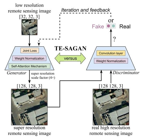
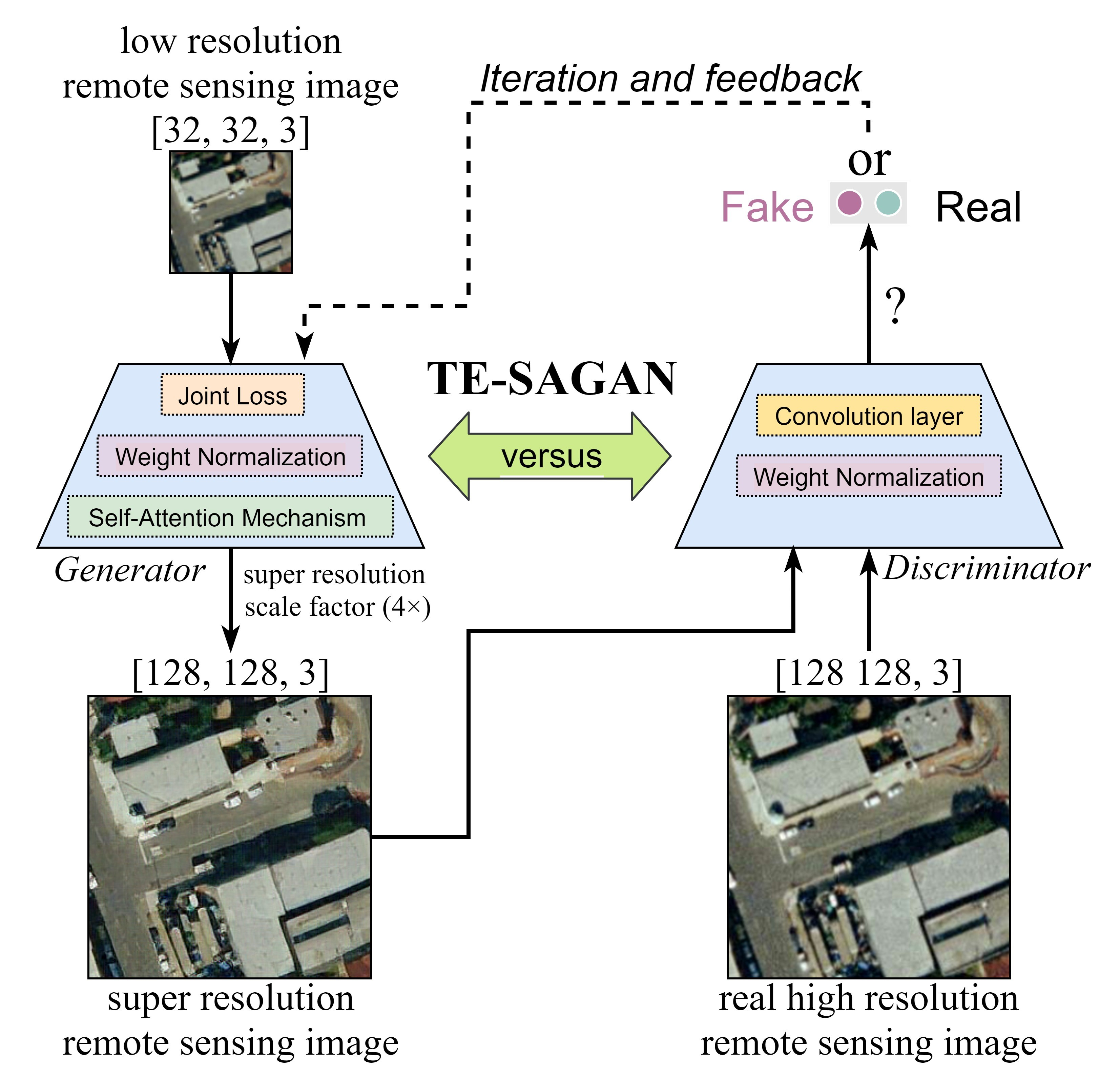
The basic idea expressed in the above equation is that the generator network G should be well-trained under the GAN (Figure 1). The discriminator network D has to distinguish the true and false states of the input remote sensing images. For the inputted , the generator in the latter term emulates the sample from the true sample , thereby minimizing the probability that the discriminator distinguishes as a fake sample. The network parameters are updated iteratively under strict monitoring conditions (e.g., loss constraints of mean square error [MSE] and mean absolute error [MAE]). The ability of the generator to fit the simulation is continuously enhanced, making it difficult for the discriminator to distinguish the reliability of the input samples. The well-trained model can predict the potential frequency distribution of the samples and generate new high-quality data sources.
2.2. Generator of TE-SAGAN
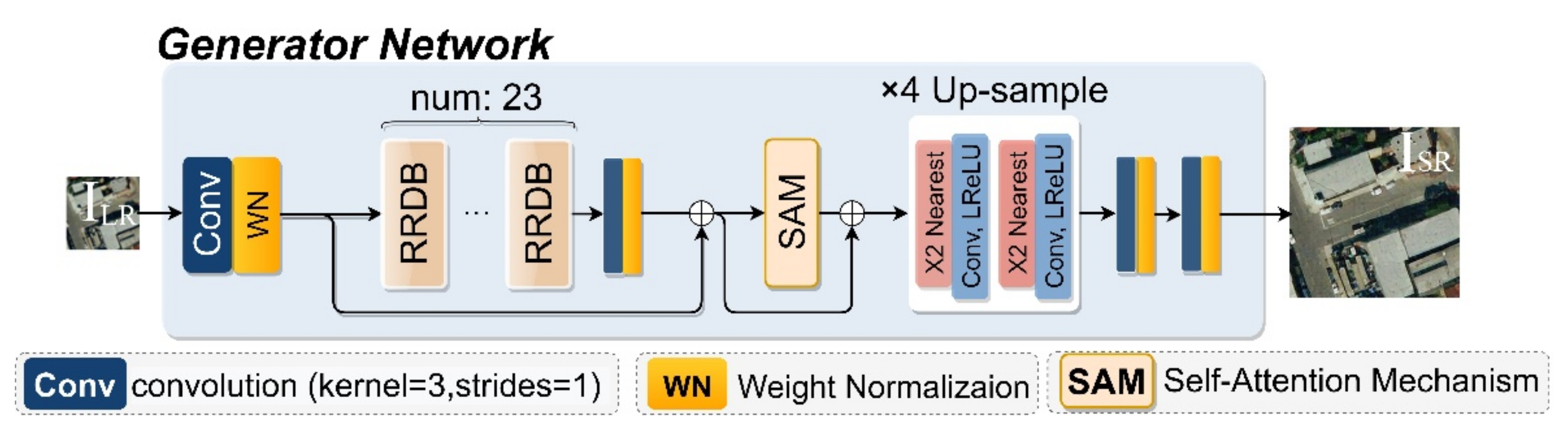
Owing to the limitation of “local perception” in conventional convolution modules, long-distance global information cannot be used for HR remote sensing images. To extract more edge and global information from remote sensing images, the generator of TE-SAGAN was designed with a low-frequency feature extractor, deep residual dense block, self-attention module, and WN (Figure 2). The self-attention module was designed to further enhance the ability of the network to extract global object features. Compared with the common batch normalization (BN) usually used in neural networks, the WN introduced in this study can stabilize network training and remove image artifacts.
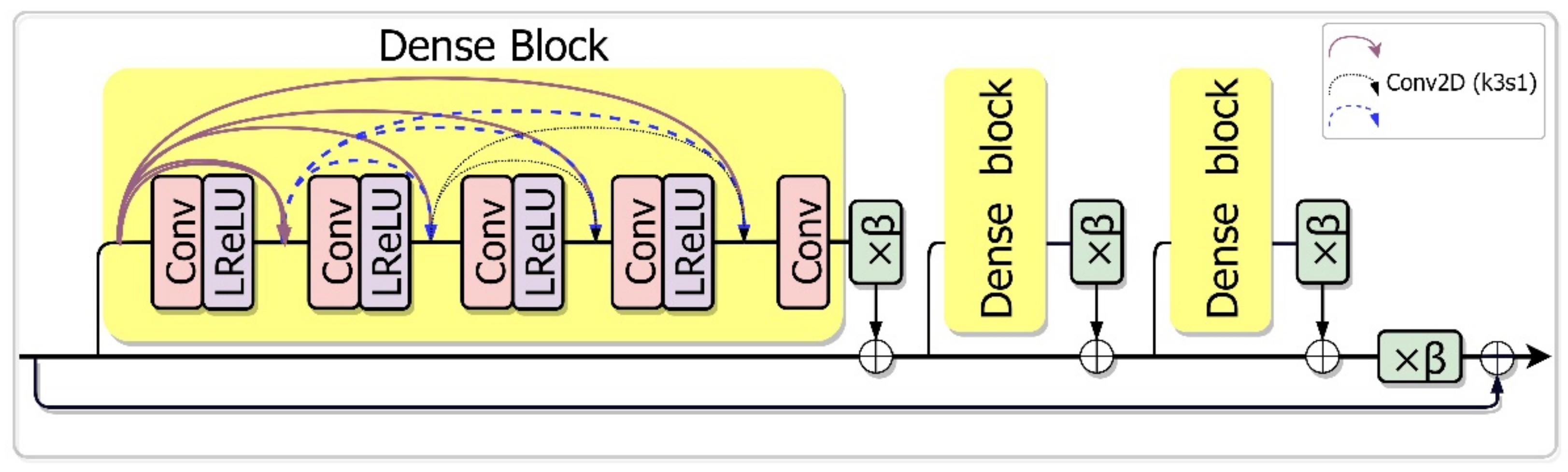
In the generator network, the low-frequency feature extractor is a convolution layer with 3 × 3 kernels, following a WN layer. RRDB is an excellent nonlinear feature extraction module that has an interwoven ensemble with dense connectivity and residual skipping. RRDB can learn deep semantic features while improving low-level feature extraction. Here, we gathered the feature-flow output from RRDB with the previous residual layer, merging them into the SAM module to generate global contextual outlines. To achieve the SR processing for remote sensing images with upscaling factors (4×), these extracted features were recovered using an up-sample layer with nearest-neighbor interpolation. In this process, in addition to keeping 23 RRDBs with the residual scaling factor and a self-attention mechanism module, each regular convolution layer was followed by WN (Figure 3).
2.2.1. Self-Attention Mechanism
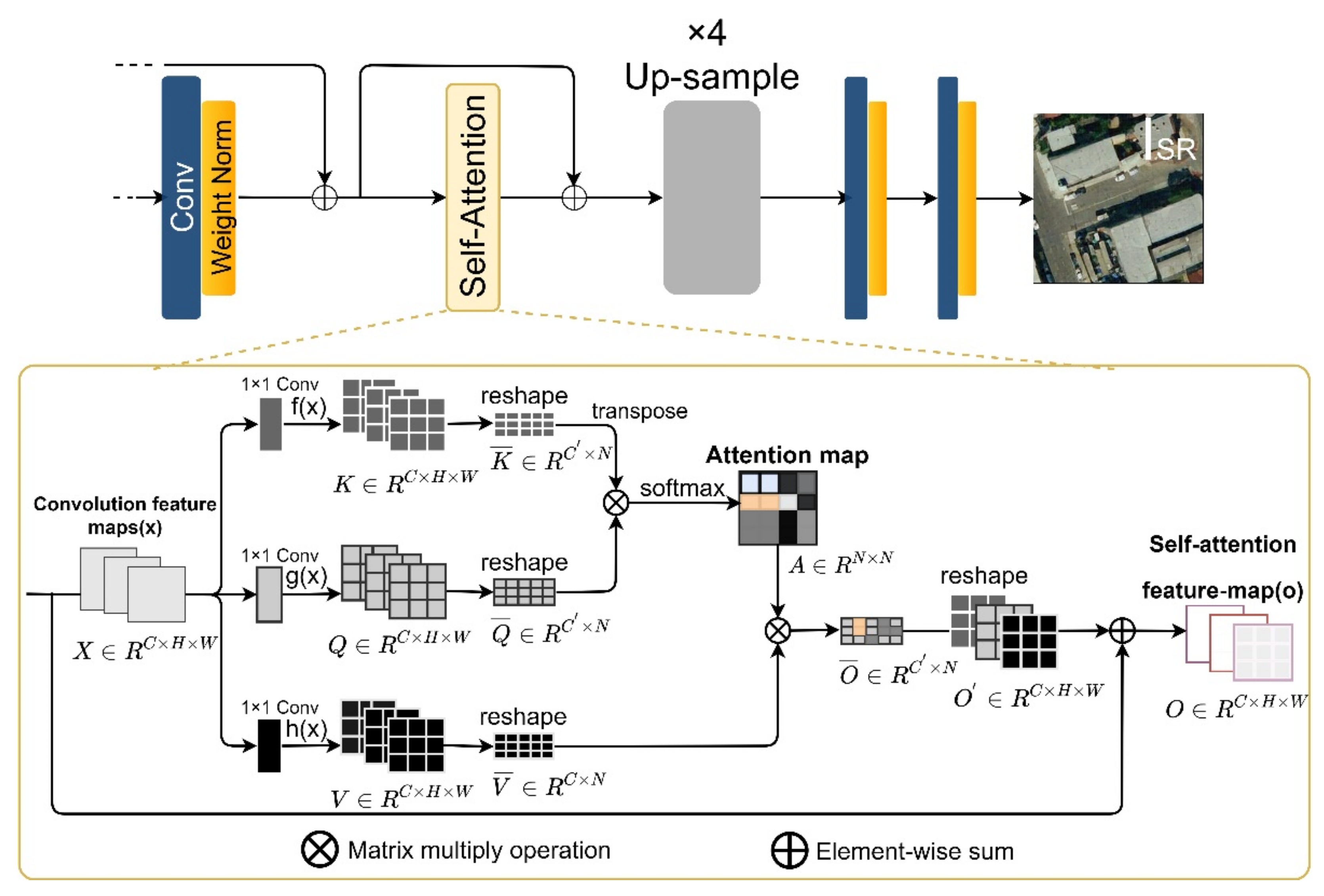
Traditional convolution operations associate regional pixels with neighboring pixels using a constant convolution kernel size. However, the limited convolution layer perception domain leads to the failure of global feature extraction, and consequently, the reconstructed image appears as a blurred overlay, or the recovered features do not correspond to the original image. Although expanding the convolution kernel size and deepening the convolution layers can help obtain the relevant global features, the computational complexity of the network increases exponentially. In recent years, attention mechanisms [41] have been widely used in natural language processing. In particular, the SAM module focuses selectively on significant location features to reduce network capacity and improve network computation performance. To obtain more global information, we designed a SAM module in the generator network (Figure 4).
The SAM module converts the previous feature nodes into three mapping sub-layers: a pixel feature extraction space , a global feature extraction space , and a convolution feature mapping layer . To improve memory efficiency, the channel number was set to . We first transposed the multiplication between and . Subsequently, the transformed softmax classification function was used to obtain the feature attention map as follows:
where indicates the significance of the synthetic j-th region model for the i-th position, , producing a series of attention map layers , where one layer is shown as:
Finally, the attention map and feature mapping layer were added together to merge the globally relevant features. The output of the layer is expressed as follows:
To explore local spatial information, was initialized as 0. Overall, self-attention can capture accurate image features beyond the convolution operation, and spatial connections between reference pixels across distances can help obtain more reference information. Furthermore, it also considers the key features of a high-resolution image with low computational complexity.
2.2.2. Weight Normalization
Batch Normalization (BN) [42] is a technique widely used in GAN-based methods. It balances the bias for image feature covariates inside the deep network and prevents overfitting during training. Nevertheless, BN tends to destroy low-frequency spatial features and increase erroneous noise estimates, causing artifacts in the SR processing results of remote sensing images. To overcome this issue, Salimans et al. have actively advocated for Weight Normalization (WN) [39] to stabilize the generative network, especially in GANs, by decoupling training weight vectors from their directions. WN decreases the dependence between mini-batch data and training performance, retains the contrast of image feature information, and has lower computational complexity than BN in equal time. Therefore, WN is more suitable than BN for performing SR tasks.
For nonlinear processing in the neural network, as seen in Equation (7), the former feature node was computed with convolutional filtering with parameters and . New feature maps and nodes were obtained by the activation function. WN in the convolution layer can be calculated using Equation (8):
where and have the same dimensional feature vector, and denotes the Euclidean norm of , which represents the direction of . Scalar g determines the length w. After WN, the neural network nodes can be calculated as follows:
2.3. Discriminator of TE-SAGAN
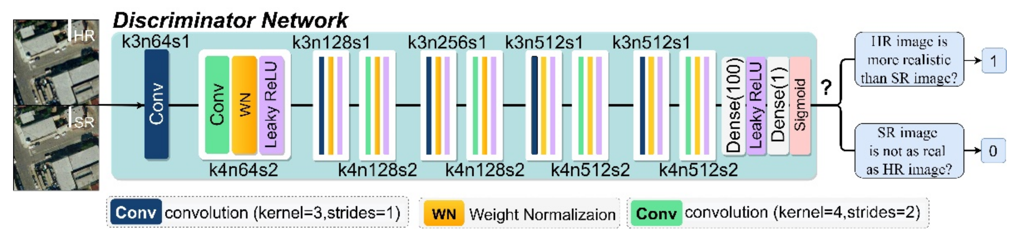
The role of the discriminator is to recognize the input images and judge their authenticity. The discriminator for TE-SAGAN is a VGGNet-type network structure [43] (Figure 5). This network has proven that multiple small convolution kernels (3 × 3) can learn more complex features at a lower computational cost than large convolutional kernels (e.g., 5 × 5, 7 × 7, and 11 × 11 in AlexNet) [44]. In this study, the fixed convolutional kernel size of VGGNet was modified to alternative kernel sizes of 3 and 4 to enhance the image feature recognition. Furthermore, the WN layers that replace all BN layers in the discriminator network can further improve the training network speed and stability.
The restored 128 × 128 SR and HR images were fed into the discriminator network. The image feature transferred through 10 layers of alternate convolution with kernel sizes of 3 × 3 and 4 × 4, step sizes of 1 and 2, and two linear dimensionality reduction operations. The channel numbers of the alternate convolution layers were 64, 128, 256, and 512. The generated feature map result was then sent into the final sigmoid function, outputting the authenticity of the remote sensing images.
2.4. Loss Function
The loss function measures the difference between the SR images generated by the network model and the HR images used for training the networks. In this study, to obtain a better result with more texture information and consistent style by TE-SAGAN, the loss function during training network combined L1 norm content loss, training adversarial network loss, perceptual loss using a high-frequency network layer from VGGNet19, and texture loss computed using the Gram matrix.
2.4.1. Content Loss
Minimization of the MAE can enhance the sensitivity of abnormal image pixels. Therefore, it was used to describe the consistency of the low-frequency data between the recovered SR image and the original HR image. The definition of content loss is:
where and jointly form the i-th pair of the training sample set, and M represents the number of training dataset pairs. is a mapping function between LR and SR images.
2.4.2. Adversarial Loss
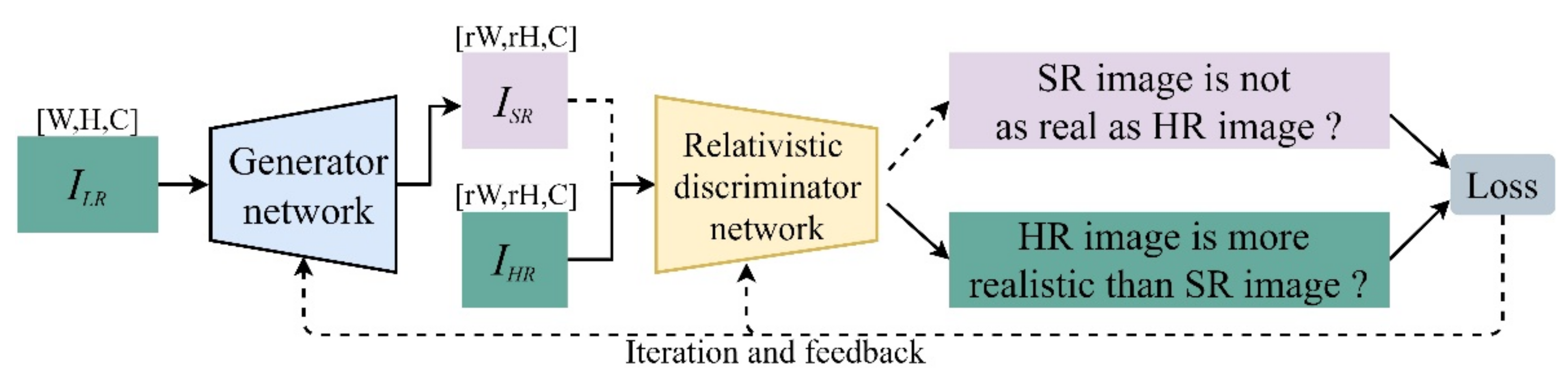
The training stability of GANs is a measure used to ensure the quality of a generated image. The generator network “pretends to learn well” to cheat the discriminator and then yields terrible results. In this experiment, we employed the relativistic average standard GAN (RasGAN) [45], an adversarial training strategy with a relativistic discriminator, to compare the average input real data relative to faked data with a more realistic probability. The adversarial TE-SAGAN loss is unlike the rule of “either true or false” in the standard GAN discriminator. Instead, it focuses on the prediction of ground truth images to improve the network robustness. The generator and discriminator loss functions have mutual symmetry, and the corresponding loss functions of TE-SAGAN are defined in Equations (11) and (12):
where denotes the original ground truth sample, , which is the generated SR remote sensing image, and represents the mean value of the generated remote sensing image for computation in the mini-batch. The adversarial loss of the generator is expressed as follows:
2.4.3. Perceptual Loss
Typically, the pixel-wise loss (MSE or MAE) is restricted to the outcomes of low-frequency smooth features. However, it has some disadvantages for sparse and weak image feature values, leading to a low supervision capability for high-frequency features. To improve the quality of the generated HR remote sensing images and enhance the robustness of the deep network, perceptual loss was calculated using high-frequency feature maps before the activation operation, which can better represent the consistency of image texture information. In the pretrained VGG19 network [43], we calculated the Euclidean metric of high-frequency features extracted before the ReLU activation layers between the reference ground truth and the reconstructed SR image, defining their differences as perceptual loss:
where represents the dimension of the feature map in the VGGNet, represents the LR remote sensing image, represents the HR remote sensing image, indicates the activation operation of the feature map extracted before the j-th convolution layer and the i-th maximum pooling layer within the VGGNet19.
2.4.4. Texture Loss
Texture is also known as low-contrast fine detail. For SR remote sensing images, restoring the texture information to approach that of HR images is the primary objective. Consideration of perceptual loss improved the quality of the reconstructed image. However, the fine textures were still obscured. In this study, based on perceptual loss, the correlation between various feature channels was used to calculate texture loss. Texture loss can consolidate and correct the details of remote sensing images. Texture loss in HR-SR images can be calculated as follows:
where represents the extracted features from VGGNet19, and is the feature map matrix computed on the gram matrix with the property of .
2.4.5. Total Loss Function
Combined with the losses described in the previous sections, the total loss function is as follows:
where and denote adversarial loss. denotes the perceptual loss mentioned in Section 2.4.3. denotes the texture loss that describes the feature details. Accordingly, , , and are the coefficients that balance different sub-loss terms.
3. Experiment and Analysis
3.1. Evaluation Indexes
The peak signal-to-noise ratio (PSNR), structural similarity (SSIM) [46], and Fréchet Inception Distance (FID) [47] scores were used as objective evaluation indices for the experimental results, whereas the visual effect provided a subjective judgment. The PSNR was used to measure the pixel difference between the compressed image or signal reconstruction image and the original image in dB. A higher PSNR score indicates higher quality and pixel fidelity of the reconstructed image. The PSNR was calculated as follows:
where represents the maximum pixel value ( is 255 for RGB images), and MSE represents the mean square error for images I and K with a size of m × n.
SSIM is a measure of luminance, contrast, and structure between two images in noise interference distortion. SSIM was calculated as follows:
where and represent the pixel mean of images x and y, respectively; represents the covariance of images x and y; naturally, and , respectively, represent the corresponding variance in images x and y. and are constants that avoid dividing by zero. Furthermore, is the range of image pixel fluctuation. and are set orderly to 0.01 and 0.03 by default. SSIM consists of the following three components:
Luminance: ;
Contrast: ;
Structure: , with .
In addition, the FID score, a proven systematic and convincing metric, was employed in this study to evaluate the accuracy of the designed model. FID computes the Fréchet distance (also known as Wasserstein-2 distance) between two Gaussian distributions (synthetic and real images) in the feature space [48]. FID constructs Gaussian model parameters around the matrix of two variables: the mean and covariance values , which refer to the mean and covariance in HR and generated images . The FID score was determined as follows:
where indicates the sum of the image features on the main diagonal of the square matrix. Accordingly, a lower FID value indicates that the produced image is closer to the HR sample.
3.2. Experiment Preparation
3.2.1. Data Set
The study area is located in the port city of Portsmouth, eastern Virginia, USA, and comprises water systems, houses, roads, and other landscape features. We built a dataset with 60,000 HR satellite image patches of 128 × 128 pixels without overlapping areas. The final 10,000 images were available for testing the trained model (called the Test-10000 set). Because the designed model’s aim is to obtain the single images’ super-resolution, the 4× super-resolution image processing is applied in this research, which is widely recognized in the current deep learning remote sensing image super-resolution tasks [49,50,51]. We used bicubic down-sampling with a common factor (4×) to obtain corresponding LR image patches and to establish a training dataset pair with HR image patches. In addition, given that super-resolution tasks primarily involve scaling of spatial resolution, the training dataset was only enhanced by random horizontal left and right flips, as well as 90°, 180°, and 270° rotations. Additionally, a well-known and publicly available dataset, the UC Merced Land Use dataset [52], was used in the test experiments. This dataset consisted of 256 × 256 pixels original HR image patches with 21 categories of satellite image scenes, each containing 100 patches of images. We selected the harbor, runway, airplane, and building scenes to validate the performance of the proposed method. Corresponding LR image patches of 64 × 64 pixels were obtained through the same down-sampling method.
3.2.2. Experimental Settings
All SR processing algorithms were implemented based on the TensorFlow framework in an Ubuntu 20.04.0 LTS system equipped with an NVIDIA GeForce RTX 2080 Ti GPU, CUDA10.1, and CUDNN7.6.0. As in a previous study [35], the training process was divided into two stages: pretraining and training. First, the proposed networks were trained with the L1 loss to consolidate the low-frequency image content and enhance the generator simulation capability. After pretraining, formal adversarial training was initialized with the parameters obtained from the final pretrained model. The balancing loss term coefficients in Equation (16) were , , and . The batch size of the imported training data was set to 16 in the pretraining phase and 4 in the adversarial training phase. The initial learning rate was set at , and half-decayed every during the pretraining phase and every during the training phase. Adam was used for the overall training optimization [53] in the training stage with default hyperparameters ( = 0.9, = 0.999).
3.3. Results and Analysis
3.3.1. Quantitative Evaluation
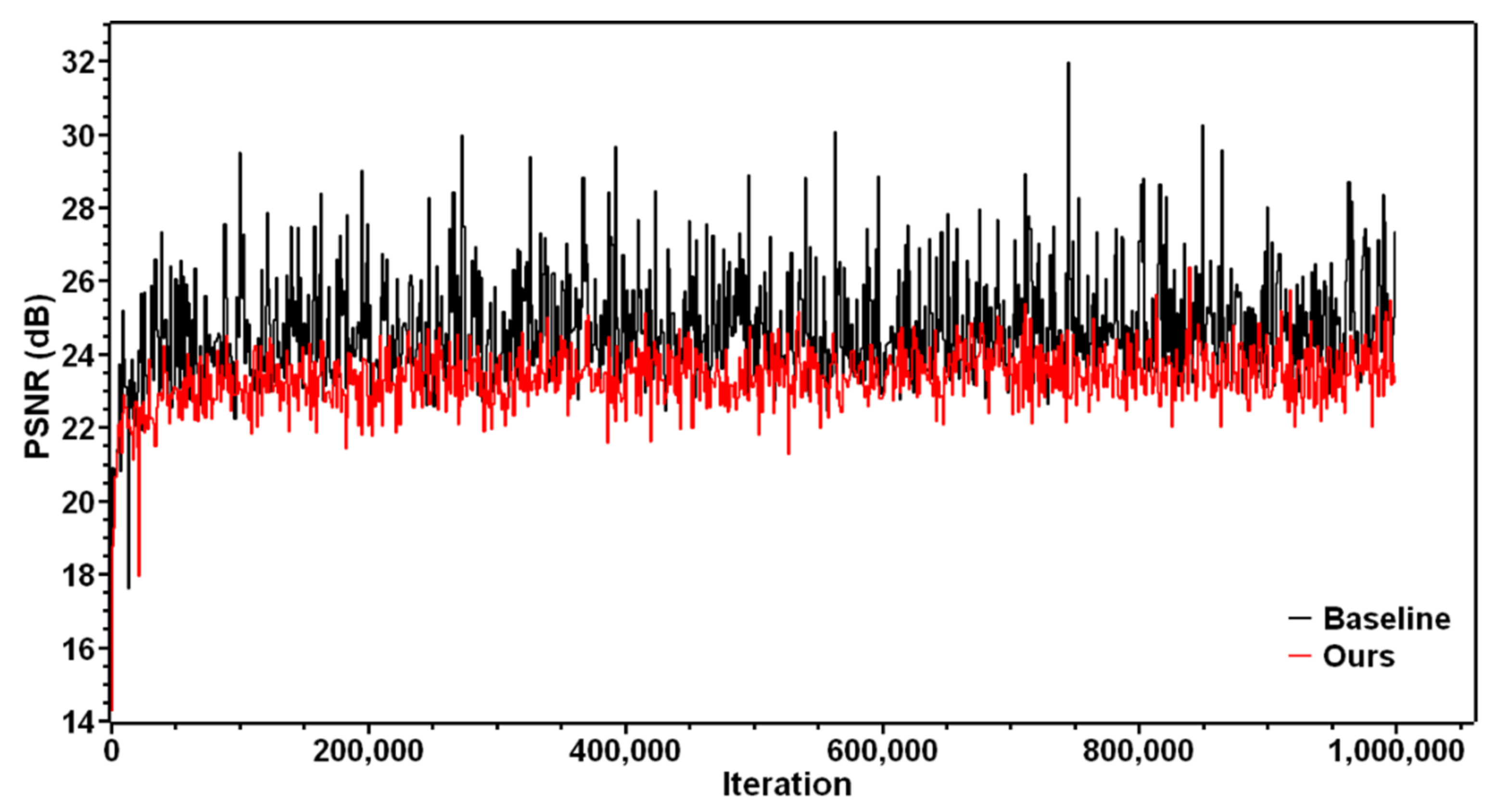
First, by comparing the results obtained using enhanced super-resolution GAN (ESRGAN) [35] and TE-SAGAN in the pretraining phase, we determined the generator network stabilization performance of the two networks. A visual example of PSNR values in the entire pretraining stage for the two methods is displayed in Figure 6. The results revealed that, compared with the baseline, the pretraining PSNR value for TE-SAGAN was slightly lower, and the network stability was considerably stronger without heavy fluctuations owing to the well-trained SAM module and WN layers.
To validate the pretrained model in detail, further experiments were conducted using remote sensing images of different scenes in the UC Merced Land Use dataset. As shown in Table 1, our method yielded better results than ESRGAN. Simultaneously, as depicted in Figure 7, the current loss function only described the low-frequency content of the image, resulting in smooth outcomes that were still not entirely convincing. We further compared several reconstructed tree shadow textures in detail and concluded that the results of the proposed model were closer to the ground truth. However, both methods produced smooth and fuzzy images in general. For alignment with human visual perception, further training using an adversarial component based on the pretrained model is necessary.
To complement prior studies, bicubic interpolation and four representative deep-learning-based SR technologies, namely, ESPCN [30], EDSR [54], SRGAN [34], ESRGAN [35], and RFDNet [55], were used as comparison methods. The quantitative comparison results are presented in Table 2. However, the mean PSNR values of our method were only 0.050 and 0.398 dB higher than the second-highest RFDNet algorithm for Test-10000 and runway, respectively. Moreover, the remaining mean PSNR values of our model were lower than RFDNet by 0.990, 0.234, and 0.205 dB for the harbor, airplane, and buildings sub-datasets, respectively, and all average SSIM scores of our model were lower than highest RFDNet by 0.017, 0.042, 0.008, 0.019, and 0.026. Instead, in the FID score term, where the lower score implies that generated images are closer to real reference images, most of the FID scores in our network were significantly lower than those in the second-lowest network, ESRGAN, by 8.816, 21.749, 7.139, and 10.580 for Test-10000, runway, airplane, and buildings, respectively, expect for the harbor sub-dataset, which was higher than RFDNet by 6.28. These findings indicate that compared with the other methods, TE-SAGAN focuses on sharpening the super resolution image while keeping a relatively high level of PSNR and SSIM image fidelity evaluations. Our method obtains a better objective rating for the four benchmark datasets. The program runtime is a non-negligible metric for evaluating network performance. ESPCN takes the shortest runtime with fast training using sub-pixel convolution, and the recent RFDNet belongs to an improved lightweight distillation network with a relatively low training runtime. Among the models with runtime lasting more than one day (1440 min), TE-SAGAN takes the shortest training time, which shortens around a quarter of the runtime than ESRGAN. The weight normalization (WN) layer introduced in this paper ensures the network stability in inputting mini-batch data to accelerate training time. Training EDSR takes the longest time. These findings indicate that TE-SAGAN shows improvement in network runtime.
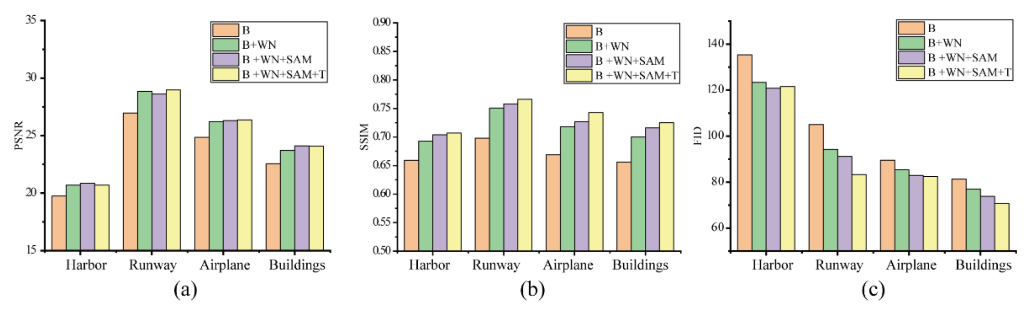
To systematically elucidate how the introduced WN and SAM affect the network performance, several TE-SAGAN ablation experiments were performed using the following networks: baseline (ESRGAN), baseline combined with the WN layer (Baseline + WN), baseline combined with the WN layer and SAM (Baseline + WN + SAM), and the final combination of SAM, WN layer, and texture loss term (Baseline + WN + SAM + Texture). Based on the results presented in Figure 8, the following conclusions were drawn. First, the addition of the WN and SAM modules to the baseline network improved the PSNR (Figure 8a) and SSIM (Figure 8b) values for several sub-datasets in the UC Merced Land Use dataset. This implies that the added modules are effective in improving the quality and fidelity of the reconstructed image. Second, the introduced texture loss focuses more on restoring texture details (FID score in Figure 8c) than on enhancing PNSR and SSIM values. Furthermore, although our network parameter was slightly larger than that of the baseline model during the experiment, our network showed higher training efficiency. In summary, the ability of WN and SAM modules to rapidly and accurately extract image features allows TE-SAGAN to reconstruct images with high fidelity, and texture loss further adds details consistent with human observation to the reconstructed image. We further believe that the added modules are associated with improved network fitness.
3.3.2. Qualitative Evaluation
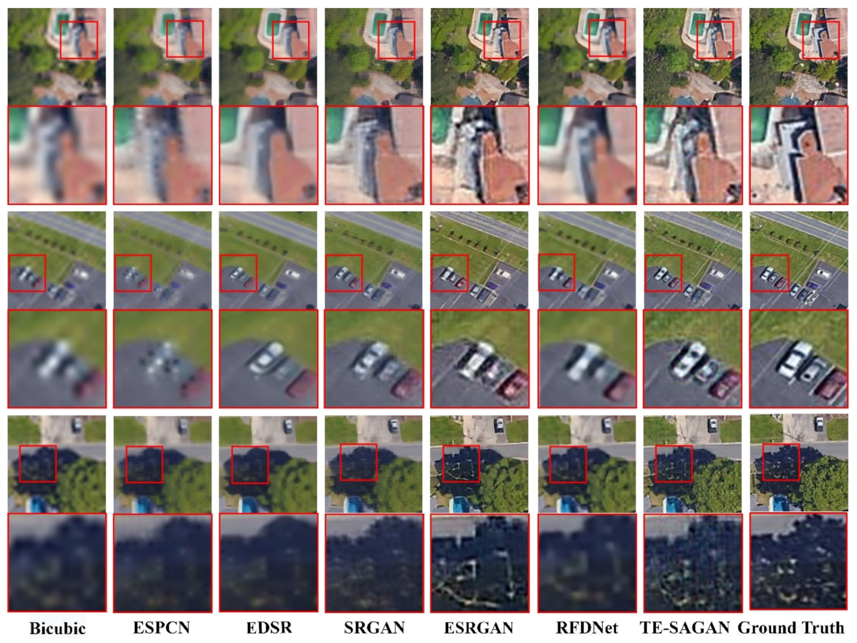
Faithful SR images has always been the focus of many image-processing tasks. As mentioned above, the PSNR and SSIM metrics obtained with the networks were different from human observations. Therefore, to further improve the texture and edge of reconstructed remote sensing images, qualitative visual comparisons were performed (Figure 9 and Figure 10). The overall quality of SR remote sensing images obtained using our method was significantly higher than those obtained via other algorithms. Figure 9 shows the processing results of our method for the test dataset (Test-10000), including the villa surroundings, car windows in the parking lot, and shade trees beside the road. In detail, bicubic interpolation [14] filled pixel information with a fixed computational paradigm, producing a blurry image. SRGAN [34] and ESRGAN [35] yielded more visually pleasant processing images than ESPCN [30] and EDSR [54] owing to their excellent depth feature extraction module and perceptual loss. However, the textures recovered by SRGAN and ESRGAN were inadequate and erroneous (e.g., car windows and tree shadows) because they lack expression and constraints on detailed and realistic textures. In particular, RFDNet is biased with respect to objective PSNR and SSIM showing higher scores, but generating super-resolution images with unclear textures. Our method was equipped with the WN layer and the Gram matrix for texture loss calculation, which significantly increased the calculation of high-frequency information correlation between SR and HR images and limited the pixel and texture deviation. Thus, our method yielded finer-grained and more realistic images.
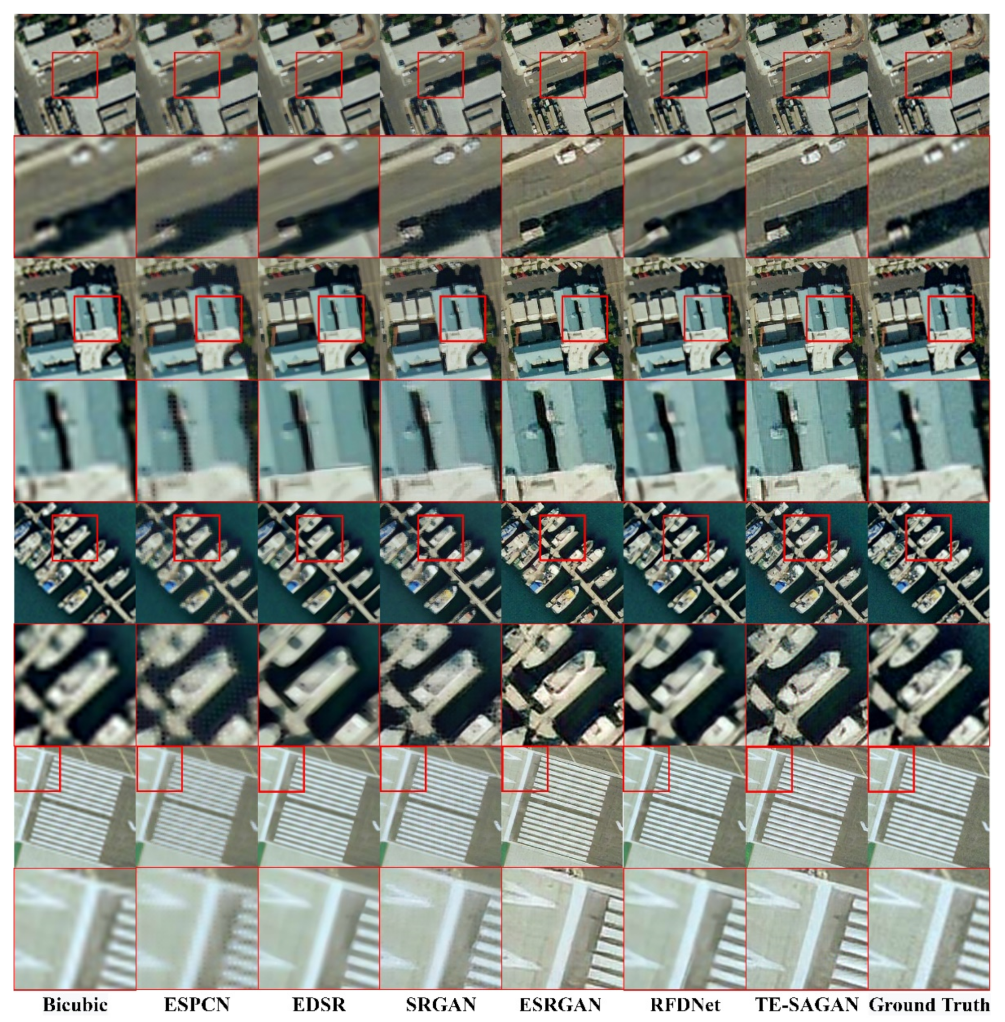
To examine the recovery status of image outlines, experiments were conducted using four representative remote sensing images from the UC Merced Land Use dataset, including street corners, rooftops, harbor ships, traffic lines, and other scenes, and the results are presented in Figure 10. SRGAN and ESRGAN produced more realistic edges than bicubic, ESPCN, EDSR, and RFDNet. However, the textures recovered by SRGAN and ESRGAN still contained unreal artifacts, as they rarely consider the spatial information of remote sensing images. In particular, RFDNet obtained high scores in objective PSNR and SSIM but generated super-resolution images with unclear outlines. In contrast, the SAM module in our proposed TE-SAGAN enhanced the connection between distant pixels, resulting in clearer, sharper edges in the reconstructed remote sensing images. Interestingly, even though several of the original HR images were slightly blurry, our method produced images with clearer and more natural borders than the original.
4. Conclusions
SR images have been widely applied for extracting information from remote sensing images. In this study, we elucidated why some algorithms lose control over edges and internal textures in the reconstructed remote sensing images even after smoothing. We proposed an RRDB-based texture-enhancement network, TE-SAGAN, which integrates the SAM and WN into the GAN framework. The SAM module effectively combines wide-area and long-range image information training. The WN layer stabilizes the reconstructed image quality using mini-batch data, thereby reducing the contrast gaps and artifacts in the generated images. In addition, the Gram matrix imposes a texture loss constraint to refine the reconstructed texture. The results for PSNR, SSIM, and FID scores of TE-SAGAN during training using our own and public benchmark remote sensing image datasets indicate improved performance. This study also suggests that our proposed method yields clearer image edges and more realistic internal details compared to existing methods. Of note, the main limitation of our current study is that we focused on rebuilding texture details and borders by increasing the model parameters. Further exploratory research is needed to reduce the model size while achieving equivalent or even superior results.
Author Contributions
Y.X. and L.T. proposed the architecture design. Y.X. and A.H. performed the experiments and analyzed the data. Y.X. and W.L. wrote the paper. X.X. and Z.X. proposed the figure in this paper. Z.X. and A.H. revised the paper and provided valuable advice for the experiments. All authors have read and agreed to the published version of the manuscript.
Funding
This study is funded by the National Natural Science Foundation of China (42001340) and the Open Fund of Key Laboratory of Urban Land Resources Monitoring and Simulation, Ministry of Natural Resources (KF-2020-05-068).
Data Availability Statement
This study did not report any data.
Conflicts of Interest
The authors declare no conflict of interest.
References
- Xu, Y.; Wu, L.; Xie, Z.; Chen, Z. Building extraction in very high resolution remote sensing imagery using deep learning and guided filters. Remote Sens. 2018, 10, 144. [Google Scholar] [CrossRef] [Green Version]
- Xu, Y.; Xie, Z.; Feng, Y.; Chen, Z. Road extraction from high-resolution remote sensing imagery using deep learning. Remote Sens. 2018, 10, 1461. [Google Scholar] [CrossRef] [Green Version]
- Guo, M.; Liu, H.; Xu, Y.; Huang, Y. Building extraction based on U-Net with an attention block and multiple losses. Remote Sens. 2020, 12, 1400. [Google Scholar] [CrossRef]
- Wei, S.; Ji, S. Graph convolutional networks for the automated production of building vector maps from aerial images. IEEE Trans. Geosci. Remote Sens. 2021, 60, 5602411. [Google Scholar] [CrossRef]
- Xia, L.; Zhang, X.; Zhang, J.; Wu, W.; Gao, X. Refined extraction of buildings with the semantic edge-assisted approach from very high-resolution remotely sensed imagery. Int. J. Remote Sens. 2020, 41, 8352–8365. [Google Scholar] [CrossRef]
- Tom, B.C.; Katsaggelos, A.K. Reconstruction of a High-Resolution Image by Simultaneous Registration, Restoration, and Interpolation of Low-Resolution Images. Proc. Int. Conf. Image Process. 1995, 2, 539–542. [Google Scholar]
- Galbraith, A.E.; Theiler, J.; Thome, K.J.; Ziolkowski, R.W. Resolution Enhancement of Multilook Imagery for the Multispectral Thermal Imager. IEEE Trans. Geosci. Remote Sens. 2005, 43, 1964–1977. [Google Scholar] [CrossRef]
- He, Y.; Yap, K.-H.; Chen, L.; Chau, L.-P. A Soft MAP Framework for Blind Super-Resolution Image Reconstruction. Image Vis. Comput. 2009, 27, 364–373. [Google Scholar] [CrossRef]
- Haut, J.M.; Fernández-Beltran, R.; Paoletti, M.E.; Plaza, J.; Plaza, A.J.; Pla, F. A New Deep Generative Network for Unsupervised Remote Sensing Single-Image Super-Resolution. IEEE Trans. Geosci. Remote Sens. 2018, 56, 6792–6810. [Google Scholar] [CrossRef]
- Lei, S.; Shi, Z.; Zou, Z. Coupled Adversarial Training for Remote Sensing Image Super-Resolution. IEEE Trans. Geosci. Remote Sens. 2020, 58, 3633–3643. [Google Scholar] [CrossRef]
- Tsai, R.Y.; Huang, T.S. Multiframe Image Restoration and Registration. Adv. Comput. Vis. Image Process. 1984, 1, 317–339. [Google Scholar]
- Cover, T.; Hart, P. Nearest Neighbor Pattern Classification. IEEE Trans. Inf. Theory 1967, 13, 21–27. [Google Scholar] [CrossRef]
- Duchon, C.E. Lanczos Filtering in One and Two Dimensions. J. Appl. Meteorol. Climatol. 1979, 18, 1016–1022. [Google Scholar] [CrossRef]
- Carlson, R.E.; Hall, C.A. Error Bounds for Bicubic Spline Interpolation. J. Approx. Theory 1973, 7, 41–47. [Google Scholar] [CrossRef] [Green Version]
- Miles, N. Method of Recovering Tomographic Signal Elements in a Projection Profile or Image by Solving Linear Equations. JUSTIA Patents No. 5323007, 21 June 1994. [Google Scholar]
- Stark, H.; Olsen, E.T. Projection-Based Image Restoration. J. Opt. Soc. Am. A-Opt. Image Sci. Vis. 1992, 9, 1914–1919. [Google Scholar] [CrossRef]
- Stark, H.; Oskoui, P. High-Resolution Image Recovery from Image-Plane Arrays, Using Convex Projections. J. Opt. Soc. Am. A Opt. Image Sci. 1989, 6, 1715–1726. [Google Scholar] [CrossRef]
- Irani, M.; Peleg, S.; Chang, H.; Yeung, D.; Xiong, Y. Super Resolution from Image Sequences Super-Resolution through Neighbor Embedding. CVPR 1990, 2, 115–120. [Google Scholar]
- Unser, M.A.; Aldroubi, A.; Eden, M. Fast B-Spline Transforms for Continuous Image Representation and Interpolation. IEEE Trans. Pattern Anal. Mach. Intell. 1991, 13, 277–285. [Google Scholar] [CrossRef]
- Unser, M.A.; Aldroubi, A.; Eden, M. B-Spline Signal Processing: Part I—Theory. IEEE Trans. Signal Process. 1993, 41, 821–833. [Google Scholar] [CrossRef]
- Unser, M.A.; Aldroubi, A.; Eden, M. B-Spline Signal Processing: Part II-Efficient Design and Applications. IEEE Trans. Signal Process. 1993, 41, 834–848. [Google Scholar] [CrossRef]
- Xu, Y.; Jin, S.; Chen, Z.; Xie, X.; Hu, S.; Xie, Z. Application of a graph convolutional network with visual and semantic features to classify urban scenes. Int. J. Geogr. Inf. Sci. 2022, 1–26. [Google Scholar] [CrossRef]
- Dong, C.; Loy, C.C.; He, K.; Tang, X. Learning a Deep Convolutional Network for Image Super-Resolution. In Proceedings of the ECCV 2014, Zurich, Switzerland, 6–12 September 2014. [Google Scholar]
- Denton, E.L.; Chintala, S.; Szlam, A.D.; Fergus, R. Deep Generative Image Models Using a Laplacian Pyramid of Adversarial Networks. NIPS 2015, 28, 1486–1494. [Google Scholar]
- Johnson, J.; Alahi, A.; Fei-Fei, L. Perceptual Losses for Real-Time Style Transfer and Super-Resolution. In Proceedings of the Computer Vision—ECCV 2016, Amsterdam, The Netherlands, 11–14 October 2016; Leibe, B., Matas, J., Sebe, N., Welling, M., Eds.; Springer International Publishing: Cham, Switzerland, 2016; pp. 694–711. [Google Scholar]
- Kim, J.; Lee, J.K.; Lee, K.M. Deeply-Recursive Convolutional Network for Image Super-Resolution. In Proceedings of the 2016 IEEE Conference on Computer Vision and Pattern Recognition (CVPR), Las Vegas, NV, USA, 27–30 June 2016; pp. 1637–1645. [Google Scholar]
- Li, J.; Fang, F.; Mei, K.; Zhang, G. Multi-Scale Residual Network for Image Super-Resolution. In Proceedings of the Computer Vision—ECCV 2018, Munich, Germany, 8–14 September 2018; Ferrari, V., Hebert, M., Sminchisescu, C., Weiss, Y., Eds.; Springer International Publishing: Cham, Switzerland, 2018; pp. 527–542. [Google Scholar]
- Han, W.; Chang, S.; Liu, D.; Yu, M.; Witbrock, M.; Huang, T.S. Image Super-Resolution via Dual-State Recurrent Networks. In Proceedings of the 2018 IEEE/CVF Conference on Computer Vision and Pattern Recognition, Salt Lake City, UT, USA, 18–23 June 2018; pp. 1654–1663. [Google Scholar]
- Dong, C.; Loy, C.C.; He, K.; Tang, X. Image Super-Resolution Using Deep Convolutional Networks. IEEE Trans. Pattern Anal. Mach. Intell. 2016, 38, 295–307. [Google Scholar] [CrossRef] [PubMed] [Green Version]
- Shi, W.; Caballero, J.; Huszár, F.; Totz, J.; Aitken, A.P.; Bishop, R.; Rueckert, D.; Wang, Z. Real-Time Single Image and Video Super-Resolution Using an Efficient Sub-Pixel Convolutional Neural Network. In Proceedings of the 2016 IEEE Conference on Computer Vision and Pattern Recognition (CVPR), Las Vegas, NV, USA, 26 June–1 July 2016; pp. 1874–1883. [Google Scholar]
- Kim, J.; Lee, J.K.; Lee, K.M. Accurate Image Super-Resolution Using Very Deep Convolutional Networks. In Proceedings of the 2016 IEEE Conference on Computer Vision and Pattern Recognition (CVPR), Las Vegas, NV, USA, 26 June–1 July 2016; pp. 1646–1654. [Google Scholar]
- Tai, Y.; Yang, J.; Liu, X.; Xu, C. MemNet: A Persistent Memory Network for Image Restoration. In Proceedings of the 2017 IEEE International Conference on Computer Vision (ICCV), Venice, Italy, 22–29 October 2017; pp. 4549–4557. [Google Scholar]
- Tong, T.; Li, G.; Liu, X.; Gao, Q. Image Super-Resolution Using Dense Skip Connections. In Proceedings of the 2017 IEEE International Conference on Computer Vision (ICCV), Venice, Italy, 22–29 October 2017; pp. 4809–4817. [Google Scholar]
- Ledig, C.; Theis, L.; Huszár, F.; Caballero, J.; Aitken, A.P.; Tejani, A.; Totz, J.; Wang, Z.; Shi, W. Photo-Realistic Single Image Super-Resolution Using a Generative Adversarial Network. In Proceedings of the 2017 IEEE Conference on Computer Vision and Pattern Recognition (CVPR), Honolulu, HI, USA, 21–26 June 2017; pp. 105–114. [Google Scholar]
- Wang, X.; Yu, K.; Wu, S.; Gu, J.; Liu, Y.; Dong, C.; Loy, C.C.; Qiao, Y.; Tang, X. ESRGAN: Enhanced Super-Resolution Generative Adversarial Networks. In Proceedings of the ECCV Workshops 2018, Munich, Germany, 8–14 September 2018. [Google Scholar]
- Rakotonirina, N.C.; Rasoanaivo, A. ESRGAN+: Further Improving Enhanced Super-Resolution Generative Adversarial Network. In Proceedings of the ICASSP 2020—2020 IEEE International Conference on Acoustics, Speech and Signal Processing (ICASSP), Barcelona, Spain, 4–8 May 2020; pp. 3637–3641. [Google Scholar]
- Wang, X.; Xie, L.; Dong, C.; Shan, Y. Real-ESRGAN: Training Real-World Blind Super-Resolution with Pure Synthetic Data. In Proceedings of the 2021 IEEE/CVF International Conference on Computer Vision Workshops (ICCVW), Montreal, BC, Canada, 10 October 2021; pp. 1905–1914. [Google Scholar]
- Jo, Y.; Yang, S.; Kim, S.J. Investigating Loss Functions for Extreme Super-Resolution. In Proceedings of the 2020 IEEE/CVF Conference on Computer Vision and Pattern Recognition Workshops (CVPRW), Seattle, WA, USA, 14–19 June 2020; pp. 1705–1712. [Google Scholar]
- Salimans, T.; Kingma, D.P. Weight Normalization: A Simple Reparameterization to Accelerate Training of Deep Neural Networks. In Proceedings of the 30th International Conference on Neural Information Processing Systems, Long Beach, CA, USA, 4–9 December 2017; Curran Associates Inc.: Red Hook, NY, USA, 2016; pp. 901–909. [Google Scholar]
- Goodfellow, I.J.; Pouget-Abadie, J.; Mirza, M.; Xu, B.; Warde-Farley, D.; Ozair, S.; Courville, A.; Bengio, Y. Generative Adversarial Nets. In Proceedings of the 27th International Conference on Neural Information Processing Systems, Bangkok, Thailand, 18–22 November 2020; MIT Press: Cambridge, MA, USA, 2020; Volume 2, pp. 2672–2680. [Google Scholar]
- Vaswani, A.; Shazeer, N.; Parmar, N.; Uszkoreit, J.; Jones, L.; Gomez, A.N.; Kaiser, L.; Polosukhin, I. Attention Is All You Need. In Proceedings of the 31st International Conference on Neural Information Processing Systems, Long Beach, CA, USA, 4–9 December 2017; Curran Associates Inc.: Red Hook, NY, USA, 2017; pp. 6000–6010. [Google Scholar]
- Ioffe, S.; Szegedy, C. Batch Normalization: Accelerating Deep Network Training by Reducing Internal Covariate Shift. In Proceedings of the 32nd International Conference on International Conference on Machine Learning, Lille, France, 7–9 July 2015; JMLR.org: Lille, France, 2015; Volume 37, pp. 448–456. [Google Scholar]
- Simonyan, K.; Zisserman, A. Very Deep Convolutional Networks for Large-Scale Image Recognition. arXiv 2015, arXiv:1409.1556. [Google Scholar]
- Krizhevsky, A.; Sutskever, I.; Hinton, G.E. ImageNet Classification with Deep Convolutional Neural Networks. Commun. ACM 2017, 60, 84–90. [Google Scholar] [CrossRef]
- Jolicoeur-Martineau, A. The Relativistic Discriminator: A Key Element Missing from Standard GAN. arXiv 2018, arXiv:1807.00734. [Google Scholar]
- Wang, Z.; Bovik, A.C.; Sheikh, H.R.; Simoncelli, E.P. Image Quality Assessment: From Error Visibility to Structural Similarity. IEEE Trans. Image Process. 2004, 13, 600–612. [Google Scholar] [CrossRef] [Green Version]
- Heusel, M.; Ramsauer, H.; Unterthiner, T.; Nessler, B.; Hochreiter, S. GANs Trained by a Two Time-Scale Update Rule Converge to a Local Nash Equilibrium. In Proceedings of the 31st International Conference on Neural Information Processing Systems, Long Beach, CA, USA, 4–9 December 2017; Curran Associates Inc.: Red Hook, NY, USA, 2017; pp. 6629–6640. [Google Scholar]
- Szegedy, C.; Vanhoucke, V.; Ioffe, S.; Shlens, J.; Wojna, Z. Rethinking the Inception Architecture for Computer Vision. In Proceedings of the 2016 IEEE Conference on Computer Vision and Pattern Recognition (CVPR), Las Vegas, NV, USA, 27–30 June 2016; pp. 2818–2826. [Google Scholar]
- Ma, W.; Pan, Z.; Guo, J.; Lei, B. Super-resolution of remote sensing images based on transferred generative adversarial network. In Proceedings of the IGARSS 2018–2018 IEEE International Geoscience and Remote Sensing Symposium, Valencia, Spain, 22–27 July 2018; pp. 1148–1151. [Google Scholar]
- Zhang, Z.; Tian, Y.; Li, J.; Xu, Y. Unsupervised Remote Sensing Image Super-Resolution Guided by Visible Images. Remote Sens. 2022, 14, 1513. [Google Scholar] [CrossRef]
- Guo, M.; Zhang, Z.; Liu, H.; Huang, Y. NDSRGAN: A Novel Dense Generative Adversarial Network for Real Aerial Imagery Super-Resolution Reconstruction. Remote Sens. 2022, 14, 1574. [Google Scholar] [CrossRef]
- Yang, Y.; Newsam, S. Bag-of-Visual-Words and Spatial Extensions for Land-Use Classification. In Proceedings of the 18th SIGSPATIAL International Conference on Advances in Geographic Information Systems, New York, NY, USA, 2–5 November 2010; Association for Computing Machinery: New York, NY, USA, 2010; pp. 270–279. [Google Scholar]
- Kingma, D.; Ba, J. Adam: A Method for Stochastic Optimization. Int. Conf. Learn. Represent. 2014. [Google Scholar] [CrossRef]
- Lim, B.; Son, S.; Kim, H.; Nah, S.; Lee, K.M. Enhanced Deep Residual Networks for Single Image Super-Resolution. In Proceedings of the 2017 IEEE Conference on Computer Vision and Pattern Recognition Workshops (CVPRW), Honolulu, HI, USA, 21–26 July 2017; pp. 1132–1140. [Google Scholar]
- Liu, J.; Tang, J.; Wu, G. Residual Feature Distillation Network for Lightweight Image Super-Resolution. In Proceedings of the Computer Vision—ECCV 2020 Workshops, Glasgow, UK, 23–28 August 2020; Bartoli, A., Fusiello, A., Eds.; Springer International Publishing: Glasgow, UK, 2020; Volume 12537, pp. 41–55. [Google Scholar]
Figure 1.
Schematic diagram of the super-resolution image processing in TE-SAGAN.

Figure 2.
Structure of the generator network of TE-SAGAN.

Figure 3.
Structure diagram of RRDB (convolution kernel size k = 3, stride s = 1, scaling factor ).

Figure 4.
The self-attention mechanism module structure.

Figure 5.
Schemes follow the same formatting. Structure diagram of the discriminator network, k denotes the convolutional kernel size, n denotes the number of convolutional kernel channels, and s denotes the convolutional stride.
Figure 5.
Schemes follow the same formatting. Structure diagram of the discriminator network, k denotes the convolutional kernel size, n denotes the number of convolutional kernel channels, and s denotes the convolutional stride.

Figure 6.
PSNR values in the pretraining networks. Baseline: pre-ESRGAN, the pretrain for ESRGAN; ours: pre-TE-SAGAN.
Figure 6.
PSNR values in the pretraining networks. Baseline: pre-ESRGAN, the pretrain for ESRGAN; ours: pre-TE-SAGAN.

Figure 7.
Results of SR processing using the Test-10000 dataset with a scale factor of 4 in the pretraining stage.
Figure 7.
Results of SR processing using the Test-10000 dataset with a scale factor of 4 in the pretraining stage.

Figure 8.
Ablation results of PSNR (a) ↑, SSIM (b) ↑, and FID (c) ↓ values using the UC Merced Land Use dataset. Baseline, ESRGAN; Baseline + WN, baseline combined with the WN layer; Baseline + WN + SAM, baseline combined with the WN and SAM modules; Baseline + WN + SAM + Texture, final combination of the SAM module, WN layer, and texture loss term.

Figure 9.
Image processing results of the different algorithms using the test dataset, including the details of roof, cars, and tree shadows.
Figure 9.
Image processing results of the different algorithms using the test dataset, including the details of roof, cars, and tree shadows.

Figure 10.
Comparative results of super-resolution image using the UC Merced Land Use dataset.


Table 1.
Comparison of pre-ESRGAN and Pre-TE-SAGAN using part of the UC Merced Land Use dataset.
| Dataset | Index | Pre-ESRGAN | Pre-TE-SAGAN |
|---|---|---|---|
| Harbor | SSIM | 0.800 | 0.798 |
| PSNR | 23.250 | 23.154 | |
| Runway | SSIM | 0.819 | 0.821 |
| PSNR | 30.574 | 30.724 | |
| Airplane | SSIM | 0.819 | 0.821 |
| PSNR | 28.748 | 28.800 | |
| Buildings | SSIM | 0.805 | 0.806 |
| PSNR | 26.124 | 26.138 |
Highest measures (PSNR [dB], SSIM) in bold [up-sampling scale 4×].
Table 2.
Comparison of Bicubic, ESPCN, EDSR, SRGAN, ESRGAN, RFDNet and TE-SAGAN on the Test-10000 set and part of UC Merced Land Use.
Table 2.
Comparison of Bicubic, ESPCN, EDSR, SRGAN, ESRGAN, RFDNet and TE-SAGAN on the Test-10000 set and part of UC Merced Land Use.
| Dataset | Metric | Bicubic | ESPCN | EDSR | SRGAN | ESRGAN | RFDNet | TE-SAGAN |
|---|---|---|---|---|---|---|---|---|
| Test-10000 | SSIM | 0.558 | 0.500 | 0.564 | 0.539 | 0.575 | 0.600 | 0.583 |
| PSNR | 22.854 | 22.141 | 22.855 | 22.695 | 23.500 | 23.650 | 23.700 | |
| FID | 136.312 | 148.199 | 95.226 | 55.252 | 32.587 | 81.866 | 23.771 | |
| Harbor | SSIM | 0.716 | 0.635 | 0.668 | 0.618 | 0.659 | 0.749 | 0.707 |
| PSNR | 20.314 | 19.339 | 19.302 | 18.814 | 19.765 | 21.760 | 20.770 | |
| FID | 147.225 | 169.257 | 205.605 | 227.557 | 135.349 | 115.247 | 121.527 | |
| Runway | SSIM | 0.704 | 0.668 | 0.678 | 0.708 | 0.698 | 0.756 | 0.748 |
| PSNR | 26.010 | 25.393 | 26.863 | 26.794 | 26.959 | 28.069 | 28.467 | |
| FID | 146.718 | 191.391 | 132.028 | 116.549 | 105.031 | 106.095 | 83.282 | |
| Airplane | SSIM | 0.713 | 0.662 | 0.709 | 0.677 | 0.669 | 0.752 | 0.733 |
| PSNR | 25.421 | 23.861 | 24.561 | 23.992 | 24.849 | 26.53 | 26.296 | |
| FID | 179.435 | 201.591 | 158.942 | 143.521 | 89.532 | 119.773 | 82.393 | |
| Buildings | SSIM | 0.699 | 0.625 | 0.670 | 0.643 | 0.656 | 0.746 | 0.720 |
| PSNR | 23.226 | 21.695 | 22.137 | 21.787 | 22.559 | 24.21 | 24.005 | |
| FID | 127.26 | 140.786 | 149.487 | 122.78 | 81.284 | 118.870 | 70.704 | |
| Runtime (min) | / | 107.8 | 3225.6 | 2292.0 | 3072.9 | 251.8 | 2288.7 |
For PSNR [dB] and SSIM , the highest values are in bold, whereas the second-highest values are underlined. On the contrary, for FID , the lowest values are in bold, whereas the second-lowest values are underlined.
Publisher’s Note: MDPI stays neutral with regard to jurisdictional claims in published maps and institutional affiliations. |
© 2022 by the authors. Licensee MDPI, Basel, Switzerland. This article is an open access article distributed under the terms and conditions of the Creative Commons Attribution (CC BY) license (https://creativecommons.org/licenses/by/4.0/).
Share and Cite
MDPI and ACS Style
Xu, Y.; Luo, W.; Hu, A.; Xie, Z.; Xie, X.; Tao, L. TE-SAGAN: An Improved Generative Adversarial Network for Remote Sensing Super-Resolution Images. Remote Sens. 2022, 14, 2425. https://0-doi-org.brum.beds.ac.uk/10.3390/rs14102425
AMA Style
Xu Y, Luo W, Hu A, Xie Z, Xie X, Tao L. TE-SAGAN: An Improved Generative Adversarial Network for Remote Sensing Super-Resolution Images. Remote Sensing. 2022; 14(10):2425. https://0-doi-org.brum.beds.ac.uk/10.3390/rs14102425
Chicago/Turabian StyleXu, Yongyang, Wei Luo, Anna Hu, Zhong Xie, Xuejing Xie, and Liufeng Tao. 2022. "TE-SAGAN: An Improved Generative Adversarial Network for Remote Sensing Super-Resolution Images" Remote Sensing 14, no. 10: 2425. https://0-doi-org.brum.beds.ac.uk/10.3390/rs14102425
Note that from the first issue of 2016, this journal uses article numbers instead of page numbers. See further details here.