Article

Mapping Fire Susceptibility in the Brazilian Amazon Forests Using Multitemporal Remote Sensing and Time-Varying Unsupervised Anomaly Detection

by
Andréa Eliza O. Luz
1,
Rogério G. Negri
1,2,*,
Klécia G. Massi
1,2,
Marilaine Colnago
3,
Erivaldo A. Silva
4 and
Wallace Casaca
5
1
Graduate Program in Natural Disasters, São Paulo State University (UNESP)/National Center for Monitoring and Early Warning of Natural Disasters (CEMADEN), São José dos Campos 12245-000, Brazil
2
Science and Technology Institute (ICT), São Paulo State University (UNESP), São José dos Campos 01049-010, Brazil
3
Institute of Mathematics and Computer Science (ICMC), São Paulo University (USP), São Carlos 13566-590, Brazil
4
Faculty of Science and Technology (FCT), São Paulo State University (UNESP), Presidente Prudente 19060-900, Brazil
5
Institute of Biosciences, Letters and Exact Sciences (IBILCE), São Paulo State University (UNESP), São José do Rio Preto 15054-000, Brazil
*
Author to whom correspondence should be addressed.
Remote Sens. 2022, 14(10), 2429; https://0-doi-org.brum.beds.ac.uk/10.3390/rs14102429
Submission received: 14 April 2022 / Revised: 8 May 2022 / Accepted: 13 May 2022 / Published: 18 May 2022

Abstract

:
The economic and environmental impacts of wildfires have leveraged the development of new technologies to prevent and reduce the occurrence of these devastating events. Indeed, identifying and mapping fire-susceptible areas arise as critical tasks, not only to pave the way for rapid responses to attenuate the fire spreading, but also to support emergency evacuation plans for the families affected by fire-related tragedies. Aiming at simultaneously mapping and measuring the risk of fires in the forest areas of Brazil’s Amazon, in this paper we combine multitemporal remote sensing, derivative spectral indices, and anomaly detection into a fully unsupervised methodology. We focus our analysis on recent forest fire events that occurred in the Brazilian Amazon by exploring multitemporal images acquired by both Landsat-8 Operational Land Imager and Modis sensors. We experimentally confirm that the current methodology is capable of predicting fire outbreaks immediately at posterior instants, which attests to the operational performance and applicability of our approach to preventing and mitigating the impact of fires in Brazilian forest regions.

Graphical Abstract

1. Introduction

Worldwide, wildfires comprise a phenomenon of paramount importance due to their severe economic and environmental consequences [1]. It is well-known that the origin of a fire may be natural, accidental, or even criminal [2]. However, in recent decades, climate changes and the intense human activity have substantially contributed to increasing the occurrence and severity of fire-related incidents on terrestrial biomes and ecosystems [3]. Furthermore, since fires are often used to renew pasture and cultivation areas [4], such dangerous strategies can trigger fire-caused accidents, leading to widespread fires such as those that devastated the Brazilian Amazon and Pantanal biomes in 2021 [5].
Fire in tropical forests are potentially hazardous for forest conservation and regeneration, which compromise plant species richness and vegetation biomass and structure [6].
In addition, according to the Intergovernmental Panel on Climate Change (IPCC), fire-occasioned events are considered the primary source of greenhouse gas emissions, thus deliberately contributing to global warming [7]. Moreover, as stated by Brando et al. [8] and Pan et al. [9], environmental issues such as temperature increasing, precipitation reduction, and other weather-related changes in vegetation areas are responsible for the emergence of less dense humid forest environments, which are more susceptible to fires.
Although fire monitoring represents a critically important activity, mapping the risk of fire events is a very challenging task in practice [10,11] since the success in predicting future fire outbreaks is limited by the lack of understanding of what triggers and controls the dynamics of such events [8]. Aiming at circumventing this issue, one can apply remote sensing (RS) tools, which include a vast repository of multitemporal data and robust computer vision apparatus. Indeed, new RS-based technologies have been proposed in recent years, allowing for the acquisition of reliable data over large monitored areas with high temporal frequency and affordable operating costs [12]. The increase in quantity and quality of RS data, as provided by a wide variety of sensors, favors the development of new and more robust data-driven methods for tracking, monitoring, and predicting fires [13,14].
Among the approaches devoted to detecting forest fires, the assessment of fire susceptibility is a particularly effective strategy, since it allows the forecasting of potential events as well as mapping areas of risk [15]. For example, the combination of varied RS data with the potentiality of unsupervised learning (UL) has proven to be consistent, not only for predicting wildfires [16,17,18], but also for other extreme weather incidents such as flood [19,20] and landslide [21] events. Moreover, unsupervised learning classification enables the automated extraction of knowledge from the Earth’s surface while mapping spatial domains. The works carried out by Dickson et al. [22], Kamalakannan et al. [23], and Hong et al. [15] are good representatives of fire susceptibility risk models that integrate the UL paradigm and large collections of RS images. The unification of UL-based techniques and multiple RS data sources is also advocated by Pourghasemi et al. [24], where the authors state the possibility of linking fire-prone areas with an incendiary event, including forest burning.
The problem of mapping fire vulnerability areas also appears in the context of anomaly detection (AD), where a classifier is trained to model and categorize nonconforming patterns that considerably deviate from the well-behaved image instances [25,26]. For instance, Xie et al. [27] merge geostationary earth observation and polar-orbiting data into a contextual AD model that relies on diurnal temperature adjustment schemes and classic image processing filtering such as Kalman and Otsu algorithms to detect active fire outbreaks. More recently, Coca and Datcu [28] discussed the use of AD for postfire assessment, estimating the fire-affected vegetation through multispectral imagery, while Saad [29] applied neural networks (NN) to forecast fire ignition areas in Western Africa by taking meteorological features and vegetation indices to solve a supervised learning classification problem. Such a learning paradigm was also adopted by Mohammed et al. [30], where a supervised support vector machine (SVM) and other classic machine learning methods are compared for early forest fire detection using geodata. Similarly, Gholamnia et al. [31] provide a comparative study between NN, random forest, decision trees, and SVM calibrated with data collected from a moderate resolution imaging spectrometer thermal anomalies product to estimate fire zones in Iran.
Despite the development of specific algorithms for the identification and quantification of wildfires, the RS literature still lacks robust and automatic techniques [32]. In fact, the need for eligible ground-truth data or a huge amount of annotated images for training is a challenge for most supervised learning methods, which include both machine [31] and deep learning [28] approaches. Another critical issue commonly found in most fire detection methods is related to their difficulty in simultaneously dealing with temporal data, illumination conditions, and the complexity of several spectral bands to properly work. Finally, as pointed out by Khosravi et al. [33] and Barmpoutis et al. [31], there is no definitive data-driven model that is best for certain hazards, since this strongly depends on the study area and abundance of data for that specific region.
Aiming at addressing most of the issues raised above, in this paper we propose a new methodology for mapping and quantifying fire-susceptible areas. More specifically, we design a fire mapping model as a time-varying anomaly detection problem, which is solved in terms of the unsupervised learning paradigm and the derivatives of spectral indices, computed from multitemporal remote sensing data. The proposed methodology is capable of both extracting and classifying fire-related features from different localities affected in a past period. In contrast to most fire detection and prediction systems, which usually depend on current weather information and do not consider features of local fire dynamics, our approach is independent of weather or other climatic variables, so that it only takes the local land cover temporal information to generate a fire-susceptibility inference model. We attest to the accuracy performance of the proposed methodology by investigating and assessing two real cases of forest fires in Brazil.
In summary, the main contributions of this study are:
  • The proposal of a fully automatic methodology for both mapping and quantifying fire-susceptible areas which relies on unsupervised anomaly detection, spectral indices differences, and satellite image time series towards better detecting patterns in complex data by learning from examples automatically.
  • The applicability assessment of two anomaly detection techniques as time-varying models to select the best-performing approach for the tasks of simultaneously classifying and quantifying fire-prone areas in Brazilian Amazon rainforest portions.
  • The development of an entire unsupervised training approach that integrates multiple sources of freely available satellite imagery and does not require any labeled data to generate a suitable fire detection model.
  • A comparative and statistical significance analysis for each implemented method regarding areas assigned as fire against areas of true fire for two real events of wildfires in the Brazilian Amazon.

2. Theoretical Aspects and Background

2.1. Anomaly Detection as a Classification Problem

In an elementary point-of-view, a classifier is a function F : X Y that assigns an element x from the attribute space X to a specific class in Ω   =   ω 1 , ω 2 , , ω c by setting a class indicator in a subset of natural numbers Y   =   1 , 2 , , c . Under these conditions, if x   X and y Y , y   =   F ( x ) indicates that x belongs to the class ω y .
The image classification task comprises the application of F on each pixel of a given image I . More specifically, the image I is defined on a support S N 2 , where each pixel s S is assigned to a vector x . Reciprocally, I ( s )   =   x may be used to denote the assignment between s and the vector x , giving rise to the formula C ( s )   =   ω y to express that F ( x )   =   y .
Basically, most image classification methods stand for different ways of defining F : X Y and applying it on I [34]. Supervised and unsupervised are the most usual learning paradigms adopted to model F. In the supervised approach, formulating F demands taking a set of training samples whose class indicator is known in advance. On the other hand, in the unsupervised case, the classifier does not depend on prelabeled training data so that the method accounts for automatically identifying patterns, clusters, and particular relationships over the data.
The anomaly detection problem can be understood as a particular application of unsupervised classification which aims at detecting events of rare occurrences or incidents that may conflict with a set of observations [35]. One-class support vector machine [36] and isolation forest [37] are effective representatives of anomaly detection techniques. These techniques can be appropriately fit and applied to extensive datasets with acceptable computational run time.
Such approaches have been successfully applied to detect bank frauds, verify intruders into security systems, and support medical examinations [38]. In addition, anomaly detection techniques have been used as very useful tools to cope with environmental monitoring issues [26,39,40].
Next, we briefly describe both aforementioned anomaly detection techniques, which are used to model our fire mapping methodology.

2.1.1. One-Class Support Vector Machine

Support vector machine (SVM) is a very popular classification method in remote sensing applications. Its solid mathematical formulation, simple algorithmic architecture, and high generalization capability are a few of the attractive characteristics of this well-established method [41,42].
From the original conception of SVM, different variants have been proposed, for example, Laplacian [43], transductive [44], context sensitive [41,45] and “one-class” SVMs [36]. Particularly, the one-class SVM (OC-SVM) relies on the problem of quantile estimation for anomaly detection.
Conceptually, starting from a set of observations I , the OC-SVM provides an unsupervised model that distinguishes the attribute vectors x as part of a set of nonanomalous elements according to a probability ν of false positive occurrences. Formally, we can write F : I X + 1 , 1 , where the output + 1 implies that the data input is in I and 1 otherwise. The definitive classifier, F, is given as follows:
F ( x )   =   sgn i   =   1 m α i K ( x , x i )     b   ,
where b   =   j   =   1 m α j K ( x i , x j ) to some x i I , and K ( · ,   · ) is a kernel function.
The coefficients α i , i   =   1 , , and m, are obtained by solving the following optimization problem:
min α 1 , , α m i , j   =   1 m α i α j K ( x i , x j ) s . t . α i [ 0 , 1 ν m ] i   =   1 m α i   =   1
It is worth noting that the OC-SVM is parameterized by ν [ 0 , 1 ] as well as by other parameters related to the kernel function used. Additional details on kernel functions are discussed in [46].

2.1.2. Isolation Forest

Isolation forest (IF) is one of the most recent methods applied to detect anomalies. Unlike other anomaly detection methods, IF relies on the fact that it does not depend on distance measurements or density-based models to select anomalous features in the image [47]. More precisely, IF focuses on looking for isolated anomalies rather than profiling regular patterns (i.e., nonanomalies). The anomaly characterization is performed through a set of binary decision trees, denominated “isolation trees” (IT), which are components of ensemble-type classifiers, the so-called “isolation forest”.
Two main properties are the basis of the IF classification [35]: (i) anomalous instances are minority present in a dataset; (ii) the data gather attribute values very different from those observed in regular instances. In addition, the IF method can be tuned by varying three major parameters: the number n i t of IT in the ensemble; the subsampling size m s u b of elements randomly drawn from the analyzed dataset; and the maximum depth d allowed for the IT growth.
Formally speaking, let I be a dataset whose elements x are defined on an n-dimensional space. We denote I ˜ as the set resulting from a subsampling performed on I with m s u b elements. From I ˜ , a binary decision tree is constructed where each node T, and its associated data, can be subdivided into the descendants T l and T r . Such division is accomplished by randomly choosing an attribute q { 1 , , n } and a value p, which may assume m s u b possible values. The division is then accomplished when the dataset associated with the node is greater than one; there are different values w.r.t. of the selected attribute, and the binary tree has not yet reached the maximum depth d.
We now assume that the process leading to the construction of an IT is replicated n i t times under the condition of different I ˜ , with distinct q and p selected for its construction. Therefore, as mentioned, the set of IT allows the creation of the definitive IF model.
Once the IF is properly built, a given vector x is classified as anomaly according to a root-to-leaf path length h ( x ) taken over each IT in the IF. Based on this concept, the following function is used to measure the anomaly level of x :
R ( x , m s u b )   =   2 E ( h ( x ) ) c ( n ) ,
where c ( n )   =   2 ln ( n 1 ) + ζ 2 ( n 1 ) n ; ζ   =   0.577215664 , representing an approximation for the Euler’s constant.
Therefore, whereas R ( x , m s u b ) 1 , x is characterized as an anomaly; otherwise, if R ( x , m s u b ) < 0.5 , the pattern x is considered regular. Finally, if R ( x , m s u b ) 0.5 , the whole set is classified as regular.

2.2. Spectral Indexes and Burn Detection

The use of spectral indices is a well-established, robust strategy to obtain discriminative features and useful information for a desirable set of targets [48]. These include as targets the wildfire areas captured by a remotely sensed scene, so that the indices allow the assessment of burn severity of these areas while still making use of low computational resources [49,50]. Some spectral indices traditionally used in remote sensing applications are: the normalized difference vegetation index (NDVI) [51], the normalized difference water index (NDWI) [52], and the normalized burn ratio (NBR) [53].
In general, spectral indices such as NDVI and NBR combine information from visible to shortwave-infrared spectral bands (which are sensitive to variations in color, soil composition, moisture, vegetation chlorophyll, etc.) in order to capture different characteristics of soil and vegetation areas affected by fire [54]. Moreover, it is worth mentioning that due to its low-reflectance behavior, the NBR index may be unable to distinguish water bodies and burned areas. In order to circumvent this issue, the NDWI becomes a useful index to quantify areas not associated with fires.
In more mathematical terms, let I ( s )   =   x be an attribute vector positioned at pixel s S , where x is formed by the reflectance intensities at green, red, near-infrared, and shortwave-infrared wavelengths bands, x Green , x Red , x NIR , and x SWIR , respectively. I NDVI , I NDWI , and I NBR establish the representation of image I in terms of NDVI, NDWI, and NBR spectral indices:
I NDVI   =   x NIR x Red x NIR + x Red , I NDWI   =   x Green x NIR x Green + x NIR , I NBR   =   x NIR x SWIR x NIR + x SWIR .
Notice that the above-described indices can be used as time-series images, as the difference (derivative) between two images taken at different instants may allow identifying and mapping specific events. As stated by Sobrino et al. [55], most fire mapping methods that make use of remote sensing data utilize postfire or prefire images. For example, the “delta-NBR” model ( Δ NBR ), introduced by Key and Benson [53], was designed to numerically assess the fire severity on vegetation areas by discriminating fire events as a function of the values obtained by:
Δ NBR   =   NBR ( pre )     NBR ( pos ) ,
where NBR ( pre ) and NBR ( pos ) account for the NBR index computed at two distinct instants, before and after the fire event. In our approach, burning signs are determined by values above 0.1 [53]. Moreover, a high value of derivative Δ NBR implies an elevated level of severity for burning.

3. Fire Susceptibility Mapping

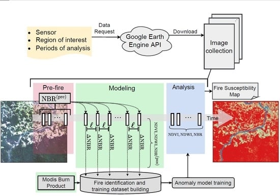
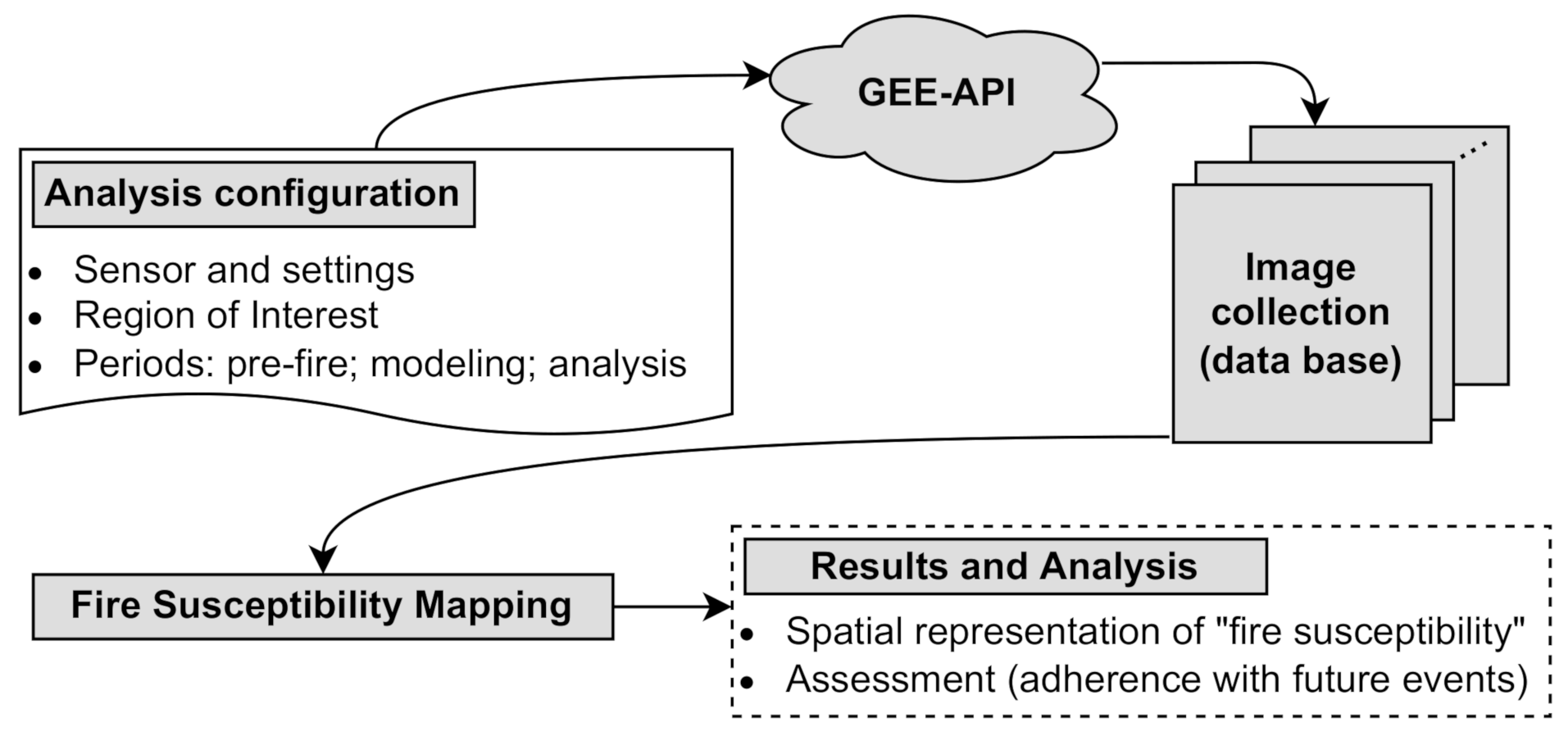
3.1. Computational Methodology

Now, we describe the main steps of the proposed methodology for mapping fire-prone areas by combining multitemporal remote sensing resources and unsupervised anomaly detection methods. Figure 1 shows an overview of the main stages of our approach, i.e., (i) analysis configuration and data acquisition, (ii) design of the fire-susceptibility mapping model, and (iii) generation of output results for analysis and validation purposes.

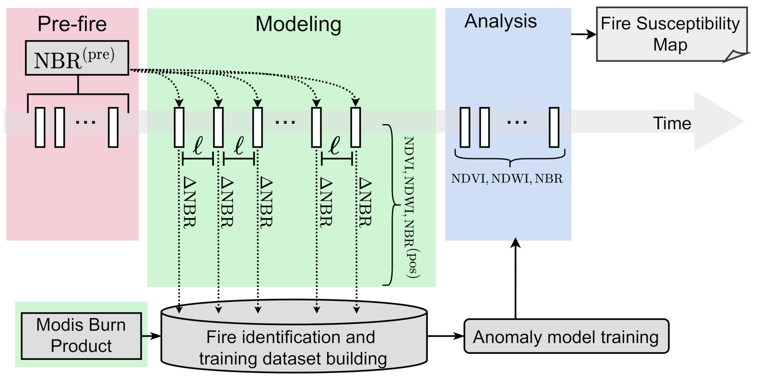
3.1.1. Multitemporal Arrangement of Remote Sensing Data

We start by describing the sequence of images taken in our study as multitemporal data, i.e., a set of remotely sensed images that were captured during three different periods.
  • Prefire period: Comprises an image series taken before the fire occurred. The goal here is to capture the central tendency at each position in the study area and then use this information to generate the NBR index as a benchmark before the presence of fire (i.e., NBR ( pre ) ) according to the Δ NBR model.
  • Modeling period: Covers a time interval whose data instances are exploited to identify fire events and, subsequently, build a time-varying anomaly detection model which learns the behavior of the fires immediately before they spread.
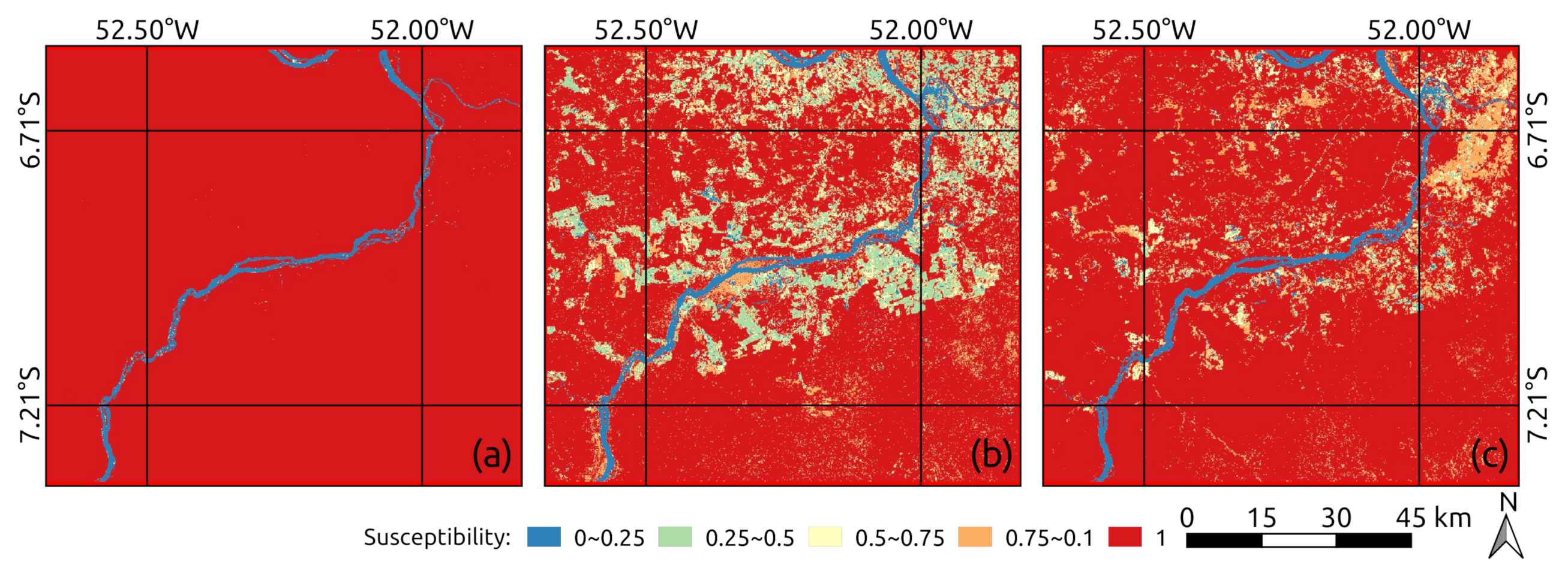
  • Analysis period: Consists of the test period, where our trained anomaly detection model is applied to classify the fire-susceptible areas.

3.1.2. Spectral Mapping, Δ NBR , and Modeling Dataset

Once the set of input images is collected, they are used to automatically build a training database, so that the unsupervised fire identification models are adjusted and generated (see Figure 2).
First, considering the image times series composed by “prefire period” data, the respective median image is computed, followed by the computation of the corresponding NBR index. As a result, the reference NBR ( pre ) is then generated. After that, concerning each instant of the “analysis period”, the NDVI, NDWI, and NBR indices are computed, where the latter is taken as NBR ( pos ) , which is used to calculate the derivative spectral index Δ NBR .
In our approach, if there is more than one image within the same time-lapse interval, we prioritize the most recent one. Moreover, areas affected by cloud/shadow occurrences are removed and recursively filled with the corresponding areas (i.e., not affected by cloud/shadow) taken from the immediately preceding instants.
The computation of Δ NBR is performed by taking the median of NBR, as calculated in the “prefire” period. In this process, the observed NBR values in the training period are taken as “postfire” (i.e., NBR ( pos ) ). From the Δ NBR computed at each instant, if it exceeds a prefixed threshold τ 0.1 (Preliminary tests show that τ 0.1 provides a suitable mapping of fire-affected locations.), then it is labeled as an event associated with fire occurrence. Aiming at minimizing false positives, the identified fire-affected areas are passed through the Modis burned area product [56]. This product, provides monthly maps with 500 m spatial resolution covering the burned areas and their respective confidence estimations. Areas that achieve Δ NBR > τ and confidence above 50%, representing a burn area in the respective period, are “double-checked” as a fire-affected location. The NDVI, NDWI, and NBR spectral indices are recorded at each fire-affected position but with respect to the immediately preceding instant.
In summary, we build a fire-prone database in a fully unsupervised fashion so that potential fire-related events are discriminated in terms of their spectral signatures and derivatives. Finally, the obtained database is used to train an anomaly detection model such as OC-SVM or IF.

3.1.3. Time-Varying Unsupervised Anomaly Detection

The anomaly detection models described in Section 2.1.1 and Section 2.1.2 are then applied on each image of the analysis period immediately after the computation of the spectral indices NDVI, NDWI, and NBR. Consequently, a collection of maps is obtained so that these mappings express the anomaly occurrences at each instant.
Notice that, in our fire mapping proposal, the identification of nonanomalous locations is interpreted as areas that demonstrate fire susceptibility. As a result, a high percentage of nonanomaly occurrences w.r.t. the number of instants in the “analysis period” at each position of the region of interest gives us the definitive fire-susceptibility map.
When the percentage values tend to 100% in a certain position, it means that such a location is similar to other fire-affected areas in all instants of the analysis period. It is important to emphasize that, once a certain AD model is built from fire-affected areas, a regular behavior (i.e., nonanomaly) is assigned to elements with areas similar to the observed fire-affected regions. Reversely, if the percentage values tend to zero, the assigned location rarely behaves like a fire-affected target, thus inferring a small susceptibility to fire.
A useful characteristic of our approach is that once the definitive model is trained, it is capable of learning the local environmental conditions, which include fire occurrences. Since this is a learned behavior, the changes occasioned by the fire incidence in a certain region make the image patterns—expressed in terms of spectral indices—less susceptible to being labeled as fire at later instants.

3.2. Data Sets, Computational Resources, and Parameter Tuning

In this section, we focus on covering a few computational aspects of our methodology as well as the data and tools used during our research.
To implement our computing prototypes, we use the Python 3.8 programming language [57]. Concerning data organization and processing, we use the Numpy [58] and Pandas [59] libraries. Finally, to train and build the OC-SMV and IF anomaly detection models, we run the Scikit-Learn [60] library.
In order to access the multitemporal remote sensing images, we adopt the Google Earth Engine application programming interface (API) [61], which is compatible with the Python language. This API favors access to high-performance computing resources for processing geospatial datasets, allowing the automation of the image search process for a given period and region of interest. The images used to define the prefire, training, and analysis periods are taken from the Operational Land Imager (OLI) sensor, onboard the Landsat-8 satellite, with 30 m of spatial resolution, 16 days of temporal resolution, and surface reflectance information from ultra-blue to shortwave-infrared wavelengths. Concerning the ancillary Modis burned area data, used to identify the fire events and build the training dataset, it comprises a 500 m resolution product containing the monthly burned area per pixel according to a confidence value [56].
The images selected to define the prefire, training, and analysis periods are limited to 50% of cloud/shadow occurrences with respect to the area comprised by the region of interest (as defined in the “analysis configuration”). This percentage level was established after a battery of preliminary tests. The cloud/shadow detection is determined by using the so-called image band “pixel_qa”. More details about this procedure are found in [62]. Regarding the parameter “time-lapse” (), once our implementation focuses on Landsat-8 images, we adopt   =   15 towards considering only one image per instant in the full time series.
As mentioned in Section 2.1, the OC-SVM and IF methods require parameters tuning. Faced with the high freedom degrees associated with the process of selecting appropriate parameters for both AD methods, we apply the well-established grid search [63] procedure to calibrate the definitive models. Basically, this procedure consists of exhaustively testing, over a defined search space, the best set of parameters that ensure higher performance. For the OC-SVM method, the search space that determines the tested settings is given by ν { 10 1 , 10 2 , , 10 7 } and an RBF kernel represented by γ { 10 1 , 10 2 , , 10 7 } . Regarding the IF parameters, we take n i t { 50 , 100 , 200 } , m s u b { d i m ( X ) , 100 % , 75 % , 50 % } , and d { 1 , 2 , , 30 } . In addition, this procedure is replicated into the decision rules of the data for each possible configuration, according to a 10-fold cross-validation process.
Finally, we freely provide the codes and data used to run our experiments at https://github.com/rogerionegri/fsm, accessed on 12 May 2022.

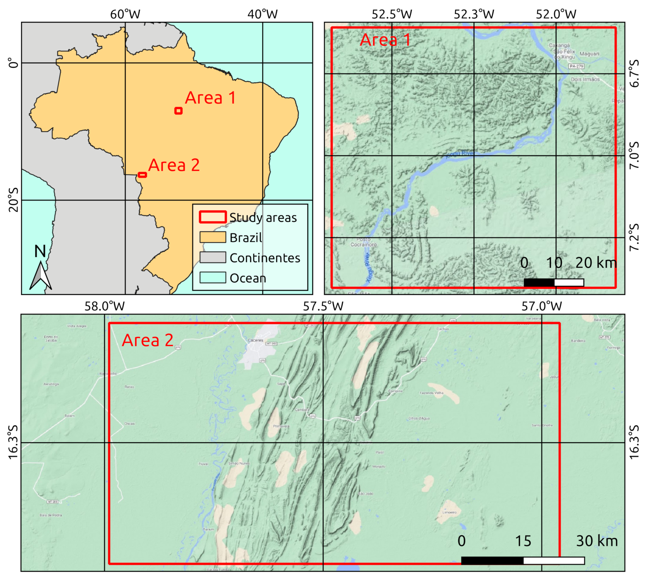
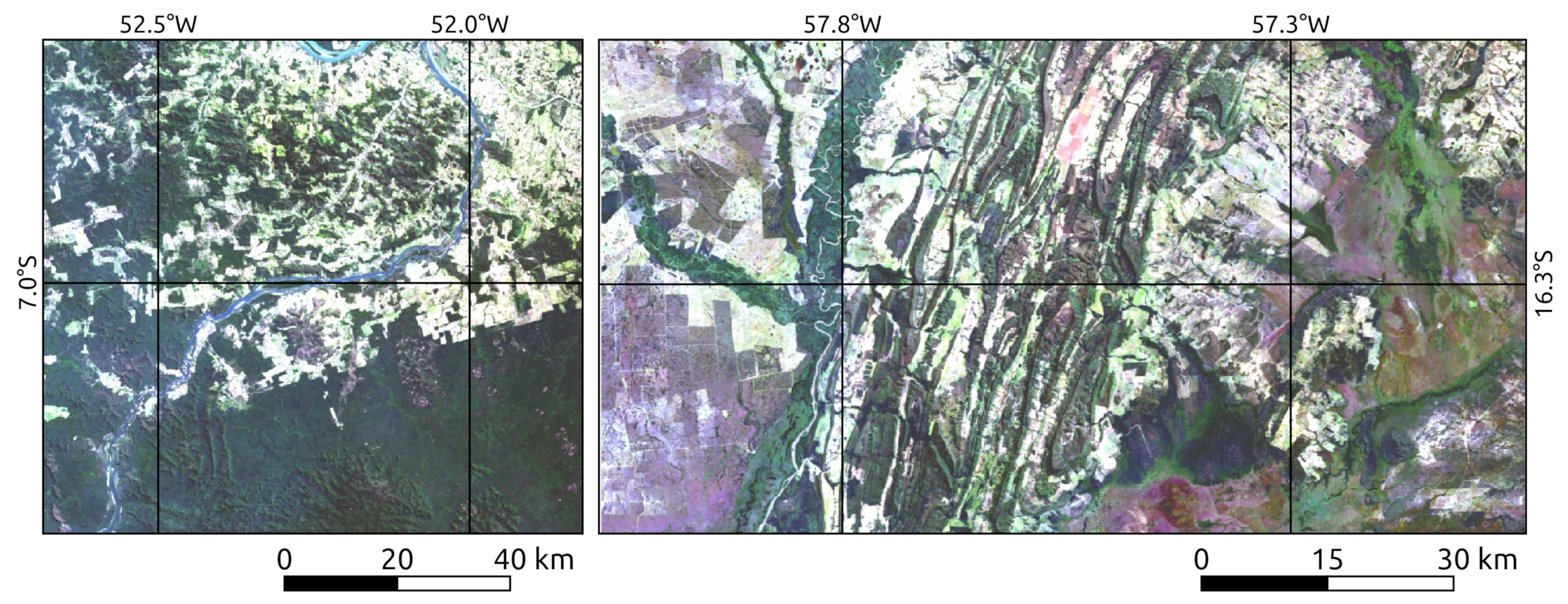
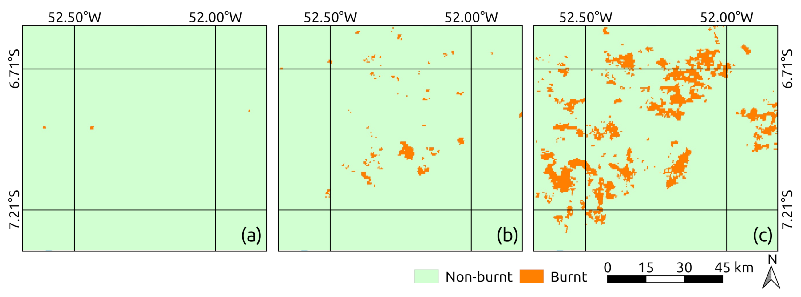
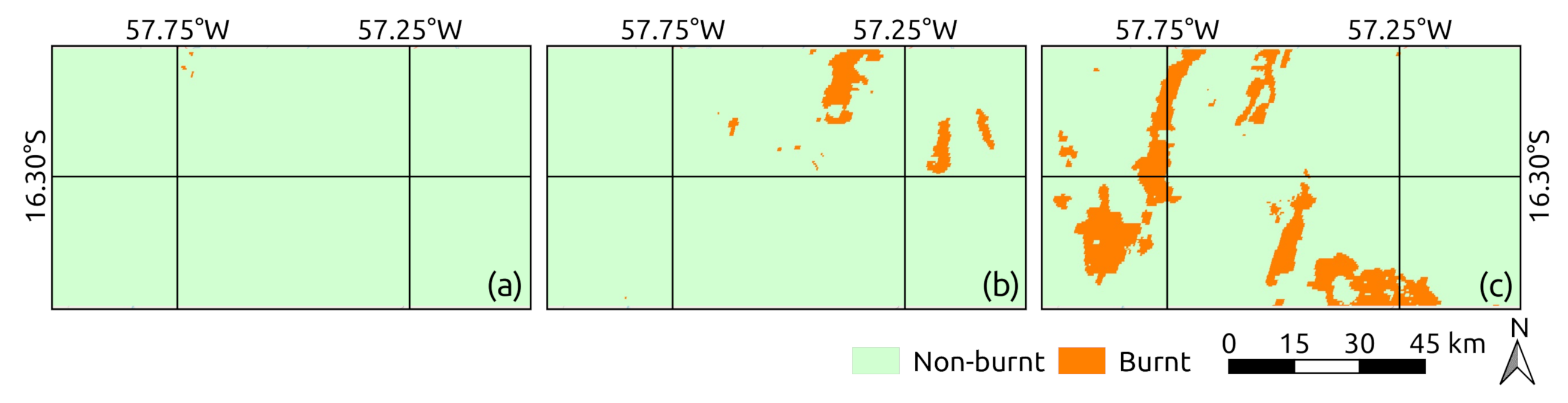
4. Study Areas and Assessment Periods

We apply the proposed methodology on two study areas and distinct epochs. Figure 3 depicts the spatial location of such regions. The first study area (Area 1) comprises an area of the Brazilian Amazon, i.e., a portion of São Félix do Xingu city, State of Pará, Brazil. The second area (Area 2) includes a portion of Cáceres city, State of Mato-Grosso, Brazil, which is another area of legal Amazon. Both areas were the scene of recent burn events with critical consequences.
Multitemporal image series registered by the OLI sensor are used as input data to the current methodology. For the sake of data exhibition, Figure 4 shows the median image computed from 1 January 2017 to 31 December 2019 regarding each study area.
The experiments comprise three distinct epochs: 2018, 2019, and 2020. Table 1 summarizes the epochs (I, II, and III) and the respective prefire, modeling, and analysis periods expressed as a function of the reference year Y. In addition, the “assessment period” shown in Table 1 stands for the burned areas registered by the Modis burned area product over the period from 1 September to 31 December Y, which are adopted to assess the fire susceptibility mappings. Figure 5 and Figure 6 present such reference dataset for Areas 1 and 2 at distinct epochs.

5. Experiments and Results

We now evaluate the current methodology for two study areas covering real fire incidents that occurred in the Brazilian Amazon rainforest from 2018 to 2020, as presented in Section 4. The obtained fire-susceptibility maps are then assessed by taking the burn events identified by the Modis burned area product as a benchmark (Figure 5 and Figure 6). For the sake of representation and comparison, the fire-susceptibility values are grouped into four classes: low [ 0 , 0.25 [ , mid-low [ 0.25 , 0.5 [ , mid-high [ 0.5 , 0.75 [ , and high [ 0.75 , 1 ] .
The experiments are conducted taking both OC-SVM and IF methods as anomaly detection models, so that the respective outputs are compared in order to determine the best fire mapping model for the investigated areas of the Amazon rainforest.
Figure 7 and Figure 8 comprise the obtained fire maps for Areas 1 and 2 at epochs I, II, and III, where the IF anomaly detection model was taken as part of our full classification methodology. Similarly, Figure 9 and Figure 10 present the results when employing OC-SVM to detect fire-prone regions. One can notice that the IF method provides more regularized mappings, i.e., results carrying fewer “isolated” pixels, when compared against OC-SVM. Targets with no burning event history are allocated in the low-susceptibility class (i.e., [ 0 , 0.25 [ ).
Notice that these targets appear as water bodies or low biomass portions, which means that such learned behavior reveals the consistency of the current approach.
The accuracy of the obtained fire-susceptibility maps can also be visually verified and assessed from the postfire events registered by the Modis burned area product (Figure 5 and Figure 6). As previously mentioned, only the burned areas are considered in our adherence analysis, so that the expected outputs should stand for high-susceptibility values.
The plots displayed in Figure 11 and Figure 12 present the observed frequencies for each susceptibility class when using the IF and OC-SVM methods, respectively. Both plotted results are quite similar to each other. As expected, the fire-affected areas (according to the adopted benchmark dataset—Figure 5 and Figure 6) are usually assigned to high-susceptibility levels (i.e., the class [ 0.75 , 1.0 ] ).
Aiming at statically assessing the significance level of the results (i.e., mid-high and high— [ 0.5 , 1.0 ] ) in comparison with the low-susceptibilities frequencies (i.e., low and mid-low [ 0 , 0.5 [ , a single-tailed (unilateral) hypothesis test for population proportion [64] was computed. Under a significance of 1%, the statistical tests reveal that the higher susceptibilities occur in proportions above 75%.
With the purpose of quantitatively comparing the susceptibility maps achieved by IF and OC-SVM at each study area and epochs, we compute 2 × 2 contingency error matrices. These reference matrices assume that the pixels of fire-affected areas, according to the Modis burn product (burn areas—Figure 5 and Figure 6), should be assigned to mid-high or high classes on the susceptibility maps, hence leading to a True Positive (TP) label. Reversely, pixels assigned to low and mid-low classes on the susceptibility maps are expected to fall within the nonburnt portions of Modis burn product images, resulting in a True Negative (TN) classification. False positives (FP) and negatives (FN) occur when expected allocations of TP or TN do not occur, respectively. For the sake of simplicity, FP and FN values are summed to indicate a global error rate, herein denoted by “False”.
Figure 13 depicts the TP, TN, and False proportions for each method and epoch. Since the number of pixels assigned to low/mid-low may change on each susceptibility map, the mentioned proportions may also change. In general, one can check that the IF method delivered slightly more False errors than OC-SVM. Nonetheless, the TP and TN proportions are quite similar for both methods regarding the results for Areas 1 and 2 in 2018 and 2019. As a result, high susceptibility regions are correctly assigned to fire-affected areas, and low-susceptibility regions are not places where fire events occur. Concerning 2020, both IF and OCSVM variants reached small False detection ratios in the period with higher occurrences of fire events (Figure 5c and Figure 6c). Moreover, the IF model achieved higher TP ratios than OCSVM in both study areas.
Additionally, we compute the F1-Score [65,66] and kappa coefficient and its variance [67] for the obtained contingency error matrices. Table 2 lists the quality metrics for both variants of our approach in all evaluation scenarios. From the tabulated kappa values for Area 1, one can verify that the OC-SVM achieves slightly better scores than IF. In terms of F1-Score, the trained models behave very similarly. Concerning Area 2, except for 2019, the IF model produced better performance. In a generalist view, it is valid to mention that the proposed methodology equipped with IF or OCSVM AD models is capable of delivering similar results.
Finally, in order to verify the statistical significance between IF and OC-SVM variants, unilateral hypothesis tests were performed to compare the kappa and variances scores. The corresponding p-values and decisions are presented in Table 3. Under a 5% level, the statistical analysis indicates that there are nonsignificant differences between the analyzed methods, except for Area 1/2019 and Area 2/2020, where OC-SVM and IF deliver the most accurate results, respectively.

6. Conclusions

In this paper, we proposed a new automatic methodology for mapping fire susceptibility in Amazon forest areas using multitemporal remote sensing images, derivative spectral indices, and unsupervised anomaly detection methods. We demonstrate the effectiveness and accuracy of the introduced approach by quantitatively as well as qualitatively analyzing two case studies covering areas heavily affected by fire in the legal Amazon forest in Brazil.
From the obtained results, we showed that the current methodology was capable of assigning a high fire-susceptibility level to the real fire-damaged areas by comparing the resulting maps with reference data representing the real fire occurrences in periods posterior to those adopted to infer the susceptibility maps. Concerning the effectiveness and consistency of IF and OC-SVM, taken as time-varying unsupervised anomaly detection techniques, we found that despite IF delivering more behaved susceptibility maps, both methods produced similar results in terms of accurateness and capability of mapping fire-prone areas.
Future perspectives for this research include: (i) adapting other anomaly detection models; (ii) taking other spectral indices as part of the anomaly detection modeling; (iii) applying the proposed methodology for other study areas; (iv) extending the implementation to other multispectral sensors such as Sentinel-2 MSI and Terra/Aqua Modis; (v) evaluating the proposed methodology through adaptations to other environmental issues, such as deforestation, floods, oil spills, melting glaciers, etc. Finally, we also intend to adapt our framework to support manually labeled data, i.e., building a semisupervised strategy. A feasible attempt could integrate labeled samples together with the conception of “cluster labeling” or even using methods such as the transduction support vector machine [68]. By doing so, we could build a training database composed of labeled data with high confidence, so that this database could be used to train anomaly detection models or even classifiers to discriminate areas susceptible to fire events in the “analysis period”.

Author Contributions

Conceptualization—A.E.O.L., R.G.N., K.G.M., M.C., E.A.S. and W.C.; Funding acquisition—R.G.N. and W.C.; Investigation—A.E.O.L. and R.G.N.; Methodology—A.E.O.L., R.G.N., K.G.M., M.C., E.A.S. and W.C.; Validation—A.E.O.L., R.G.N., K.G.M. and M.C. Writing—Original draft—A.E.O.L. and R.G.N. All authors have read and agreed to the published version of the manuscript.

Funding

This research was funded by the São Paulo Research Foundation (FAPESP), grants 2021/01305-6 and 2021/03328-3, and National Council for Scientific and Technological Development (CNPq), grants 427915/2018-0, 304402/2019-2, 316228/2021-4 and 164326/2020-0. The APC was partially funded by São Paulo State University (UNESP).

Data Availability Statement

The code of the proposed framework in Section 3.2 is freely available at https://github.com/rogerionegri/fsm, accessed on 12 May 2022.

Conflicts of Interest

The authors declare no conflict of interest. The funders had no role in the design of the study; in the collection, analyses, or interpretation of data; in the writing of the manuscript, or in the decision to publish the results.

References

  1. Artés, T.; Oom, D.; De Rigo, D.; Durrant, T.H.; Maianti, P.; Libertà, G.; San-Miguel-Ayanz, J. A global wildfire dataset for the analysis of fire regimes and fire behaviour. Sci. Data 2019, 6, 296. [Google Scholar] [CrossRef] [PubMed]
  2. Caúla, R.; Oliveira-Júnior, J.F.; Lyra, G.B.; Delgado, R.; Heilbron Filho, P. Overview of fire foci causes and locations in Brazil based on meteorological satellite data from 1998 to 2011. Environ. Earth Sci. 2015, 74, 1497–1508. [Google Scholar] [CrossRef]
  3. Cochrane, M.A.; Barber, C.P. Climate change, human land use and future fires in the Amazon. Glob. Chang. Biol. 2009, 15, 601–612. [Google Scholar] [CrossRef]
  4. Garcia, L.C.; Szabo, J.K.; de Oliveira Roque, F.; Pereira, A.d.M.M.; da Cunha, C.N.; Damasceno-Júnior, G.A.; Morato, R.G.; Tomas, W.M.; Libonati, R.; Ribeiro, D.B. Record-breaking wildfires in the world’s largest continuous tropical wetland: Integrative fire management is urgently needed for both biodiversity and humans. J. Environ. Manag. 2021, 293, 112870. [Google Scholar] [CrossRef]
  5. INPE. Instituto Nacional de Pesquisas Espaciais—Banco de Dados de Queimadas. 2021. Available online: https://queimadas.dgi.inpe.br/queimadas/bdqueimadas (accessed on 29 March 2021).
  6. Prestes, N.C.C.d.S.; Massi, K.G.; Silva, E.A.; Nogueira, D.S.; de Oliveira, E.A.; Freitag, R.; Marimon, B.S.; Marimon-Junior, B.H.; Keller, M.; Feldpausch, T.R. Fire effects on understory forest regeneration in southern Amazonia. Front. For. Glob. Chang. 2020, 3, 10. [Google Scholar] [CrossRef]
  7. Field, C.B.; Barros, V.; Stocker, T.F.; Dahe, Q. Managing the Risks of Extreme Events and Disasters to Advance Climate Change Adaptation: Special Report of the Intergovernmental Panel on Climate Change; Cambridge University Press: Cambridge, UK, 2012. [Google Scholar]
  8. Brando, P.M.; Balch, J.K.; Nepstad, D.C.; Morton, D.C.; Putz, F.E.; Coe, M.T.; Silvério, D.; Macedo, M.N.; Davidson, E.A.; Nóbrega, C.C.; et al. Abrupt increases in Amazonian tree mortality due to drought—Fire interactions. Proc. Natl. Acad. Sci. USA 2014, 111, 6347–6352. [Google Scholar] [CrossRef] [Green Version]
  9. Pan, Y.; Birdsey, R.A.; Fang, J.; Houghton, R.; Kauppi, P.E.; Kurz, W.A.; Phillips, O.L.; Shvidenko, A.; Lewis, S.L.; Canadell, J.G.; et al. A large and persistent carbon sink in the world’s forests. Science 2011, 333, 988–993. [Google Scholar] [CrossRef] [Green Version]
  10. Birch, D.S.; Morgan, P.; Kolden, C.A.; Abatzoglou, J.T.; Dillon, G.K.; Hudak, A.T.; Smith, A.M. Vegetation, topography and daily weather influenced burn severity in central Idaho and western Montana forests. Ecosphere 2015, 6, 1–23. [Google Scholar] [CrossRef]
  11. Mann, M.L.; Batllori, E.; Moritz, M.A.; Waller, E.K.; Berck, P.; Flint, A.L.; Flint, L.E.; Dolfi, E. Incorporating anthropogenic influences into fire probability models: Effects of human activity and climate change on fire activity in California. PLoS ONE 2016, 11, e0153589. [Google Scholar] [CrossRef] [Green Version]
  12. Pereira, A.A.; Pereira, J.; Libonati, R.; Oom, D.; Setzer, A.W.; Morelli, F.; Machado-Silva, F.; De Carvalho, L.M.T. Burned area mapping in the Brazilian Savanna using a one-class support vector machine trained by active fires. Remote Sens. 2017, 9, 1161. [Google Scholar] [CrossRef] [Green Version]
  13. Yuan, Q.; Shen, H.; Li, T.; Li, Z.; Li, S.; Jiang, Y.; Xu, H.; Tan, W.; Yang, Q.; Wang, J.; et al. Deep learning in environmental remote sensing: Achievements and challenges. Remote Sens. Environ. 2020, 241, 111716. [Google Scholar] [CrossRef]
  14. Martínez-Álvarez, F.; Tien Bui, D. Advanced Machine Learning and Big Data Analytics in Remote Sensing for Natural Hazards Management. Remote Sens. 2020, 12, 301. [Google Scholar] [CrossRef] [Green Version]
  15. Hong, H.; Tsangaratos, P.; Ilia, I.; Liu, J.; Zhu, A.X.; Xu, C. Applying genetic algorithms to set the optimal combination of forest fire related variables and model forest fire susceptibility based on data mining models. The case of Dayu County, China. Sci. Total Environ. 2018, 630, 1044–1056. [Google Scholar] [CrossRef] [PubMed]
  16. Leuenberger, M.; Parente, J.; Tonini, M.; Pereira, M.G.; Kanevski, M. Wildfire susceptibility mapping: Deterministic vs. stochastic approaches. Environ. Model. Softw. 2018, 101, 194–203. [Google Scholar] [CrossRef]
  17. Shirazi, Z.; Wang, L.; Bondur, V.G. Modeling Conditions Appropriate for Wildfire in South East China—A Machine Learning Approach. Front. Earth Sci. 2021, 9, 361. [Google Scholar] [CrossRef]
  18. Achu, A.; Thomas, J.; Aju, C.; Gopinath, G.; Kumar, S.; Reghunath, R. Machine-learning modeling of fire susceptibility in a forest-agriculture mosaic landscape of southern India. Ecol. Inform. 2021, 64, 101348. [Google Scholar] [CrossRef]
  19. Mirzaei, S.; Vafakhah, M.; Pradhan, B.; Alavi, S.J. Flood susceptibility assessment using extreme gradient boosting (EGB), Iran. Earth Sci. Inform. 2021, 14, 51–67. [Google Scholar] [CrossRef]
  20. Wang, H.; Zhao, Y.; Zhou, Y.; Wang, H. Prediction of urban water accumulation points and water accumulation process based on machine learning. Earth Sci. Inform. 2021, 14, 2317–2328. [Google Scholar] [CrossRef]
  21. Fallah-Zazuli, M.; Vafaeinejad, A.; Alesheykh, A.A.; Modiri, M.; Aghamohammadi, H. Mapping landslide susceptibility in the Zagros Mountains, Iran: A comparative study of different data mining models. Earth Sci. Inform. 2019, 12, 615–628. [Google Scholar] [CrossRef]
  22. Dickson, B.G.; Prather, J.W.; Xu, Y.; Hampton, H.M.; Aumack, E.N.; Sisk, T.D. Mapping the probability of large fire occurrence in northern Arizona, USA. Landsc. Ecol. 2006, 21, 747–761. [Google Scholar] [CrossRef]
  23. Kamalakannan, J.; Chakrabortty, A.; Bothra, G.; Pare, P.; Kumar, C.P. Forest fire prediction to prevent environmental hazards using data mining approach. In Proceedings of the 2nd International Conference on Data Engineering and Communication Technology, Pune, India, 15–16 December 2017; Springer: Singapore, 2017; pp. 615–622. [Google Scholar]
  24. Pourghasemi, H.R.; Kariminejad, N.; Amiri, M.; Edalat, M.; Zarafshar, M.; Blaschke, T.; Cerda, A. Assessing and mapping multi-hazard risk susceptibility using a machine learning technique. Sci. Rep. 2020, 10, 3203. [Google Scholar] [CrossRef] [PubMed] [Green Version]
  25. Li, Z.; Li, J.; Zhou, S.; Pirasteh, S. Developing an algorithm for local anomaly detection based on spectral space window in hyperspectral image. Earth Sci. Inform. 2015, 8, 741–749. [Google Scholar] [CrossRef]
  26. Dias, M.A.; Silva, E.A.d.; Azevedo, S.C.d.; Casaca, W.; Statella, T.; Negri, R.G. An Incongruence-Based Anomaly Detection Strategy for Analyzing Water Pollution in Images from Remote Sensing. Remote Sens. 2020, 12, 43. [Google Scholar] [CrossRef] [Green Version]
  27. Xie, Z.; Song, W.; Ba, R.; Li, X.; Xia, L. A Spatiotemporal Contextual Model for Forest Fire Detection Using Himawari-8 Satellite Data. Remote Sens. 2018, 10, 1992. [Google Scholar] [CrossRef] [Green Version]
  28. Coca, M.; Datcu, M. Anomaly Detection in Post Fire Assessment. In Proceedings of the IEEE International Geoscience and Remote Sensing Symposium (IGARSS), Brussels, Belgium, 11–16 July 2021; pp. 8620–8623. [Google Scholar]
  29. Saad, L. Predicting, Understanding, and Visualizing Fire Dynamics with Neural Networks. Master’s Thesis, Technical University of Munich, Munich, Germany, 2021. [Google Scholar]
  30. Mohammed, Z.; Hanae, C.; Larbi, S. Comparative Study on Machine Learning Algorithms for early fire forest detection system using geodata. Int. J. Electr. Comput. Eng. (IJECE) 2020, 10, 5507–5513. [Google Scholar] [CrossRef]
  31. Barmpoutis, P.; Papaioannou, P.; Dimitropoulos, K.; Grammalidis, N. Comparisons of Diverse Machine Learning Approaches for Wildfire Susceptibility Mapping. Symmetry 2020, 12, 604. [Google Scholar]
  32. Ban, Y.; Zhang, P.; Nascetti, A.; Bevington, A.R.; Wulder, M.A. Near real-time wildfire progression monitoring with Sentinel-1 SAR time series and deep learning. Sci. Rep. 2020, 10, 1322. [Google Scholar] [CrossRef] [Green Version]
  33. Khosravi, K.; Panahi, M.; Tien Bui, D. Spatial prediction of groundwater spring potential mapping based on an adaptive neuro-fuzzy inference system and metaheuristic optimization. Hydrol. Earth Syst. Sci. 2018, 22, 4771–4792. [Google Scholar] [CrossRef] [Green Version]
  34. Negri, R.G.; Frery, A.C.; Casaca, W.; Azevedo, S.; Dias, M.A.; Silva, E.A.; Alcântara, E.H. Spectral–Spatial-Aware Unsupervised Change Detection With Stochastic Distances and Support Vector Machines. IEEE Trans. Geosci. Remote Sens. 2021, 59, 2863–2876. [Google Scholar] [CrossRef]
  35. Akoglu, L.; Tong, H.; Koutra, D. Graph based anomaly detection and description: A survey. Data Min. Knowl. Discov. 2015, 29, 626–688. [Google Scholar] [CrossRef] [Green Version]
  36. Schölkopf, B.; Platt, J.C.; Shawe-Taylor, J.; Smola, A.J.; Williamson, R.C. Estimating the support of a high-dimensional distribution. Neural Comput. 2001, 13, 1443–1471. [Google Scholar] [CrossRef] [PubMed]
  37. Liu, F.T.; Ting, K.M.; Zhou, Z. Isolation Forest. In Proceedings of the 2008 Eighth IEEE International Conference on Data Mining, Pisa, Italy, 15–19 December 2008; pp. 413–422. [Google Scholar] [CrossRef]
  38. Gu, S.; Hu, Q.; Cheng, Y.; Bai, L.; Liu, Z.; Xiao, W.; Gong, Z.; Wu, Y.; Feng, K.; Deng, Y.; et al. Application of organic fertilizer improves microbial community diversity and alters microbial network structure in tea (Camellia sinensis) plantation soils. Soil Tillage Res. 2019, 195, 104356. [Google Scholar] [CrossRef]
  39. Dereszynski, E.W.; Dietterich, T.G. Spatiotemporal Models for Data-Anomaly Detection in Dynamic Environmental Monitoring Campaigns. ACM Trans. Sens. Netw. (TOSN) 2011, 8, 1–36. [Google Scholar] [CrossRef]
  40. Havens, T.C.; Bezdek, J.C. An efficient formulation of the improved visual assessment of cluster tendency (iVAT) algorithm. IEEE Trans. Knowl. Data Eng. 2011, 24, 813–822. [Google Scholar] [CrossRef]
  41. Bruzzone, L.; Persello, C. A novel context-sensitive semisupervised SVM classifier robust to mislabeled training samples. IEEE Trans. Geosci. Remote Sens. 2009, 47, 2142–2154. [Google Scholar] [CrossRef] [Green Version]
  42. Mountrakis, G.; Im, J.; Ogole, C. Support vector machines in remote sensing: A review. ISPRS J. Photogramm. Remote Sens. 2011, 66, 247–259. [Google Scholar] [CrossRef]
  43. Gu, Y.; Feng, K. Optimized Laplacian SVM with distance metric learning for hyperspectral image classification. IEEE J. Sel. Top. Appl. Earth Obs. Remote Sens. 2013, 6, 1109–1117. [Google Scholar] [CrossRef]
  44. Li, Y.; Wang, Y.; Bi, C.; Jiang, X. Revisiting transductive support vector machines with margin distribution embedding. Knowl.-Based Syst. 2018, 152, 200–214. [Google Scholar] [CrossRef]
  45. Negri, R.G.; da Silva, E.A.; Casaca, W. Inducing Contextual Classifications With Kernel Functions Into Support Vector Machines. IEEE Geosci. Remote Sens. Lett. 2018, 15, 962–966. [Google Scholar] [CrossRef]
  46. Shawe-Taylor, J.; Cristianini, N. Kernel Methods for Pattern Analysis; Cambridge University Press: Cambridge, UK, 2004. [Google Scholar]
  47. Liu, F.T.; Ting, K.M.; Zhou, Z.H. Isolation-based anomaly detection. ACM Trans. Knowl. Discov. Data (TKDD) 2012, 6, 1–39. [Google Scholar] [CrossRef]
  48. Kumar, A.; Bhandari, A.K.; Padhy, P. Improved normalised difference vegetation index method based on discrete cosine transform and singular value decomposition for satellite image processing. IET Signal Process. 2012, 6, 617–625. [Google Scholar] [CrossRef]
  49. Schepers, L.; Haest, B.; Veraverbeke, S.; Spanhove, T.; Vanden Borre, J.; Goossens, R. Burned area detection and burn severity assessment of a heathland fire in Belgium using airborne imaging spectroscopy (APEX). Remote Sens. 2014, 6, 1803–1826. [Google Scholar] [CrossRef] [Green Version]
  50. Veraverbeke, S.; Harris, S.; Hook, S. Evaluating spectral indices for burned area discrimination using MODIS/ASTER (MASTER) airborne simulator data. Remote Sens. Environ. 2011, 115, 2702–2709. [Google Scholar] [CrossRef]
  51. Rouse, J.W.; Haas, R.H.; Schell, J.A.; Deering, D.W. Monitoring vegetation systems in the Great Plains with ERTS. NASA Spec. Publ. 1974, 351, 309. [Google Scholar]
  52. Gao, B.C. NDWI—A normalized difference water index for remote sensing of vegetation liquid water from space. Remote Sens. Environ. 1996, 58, 257–266. [Google Scholar] [CrossRef]
  53. Key, C.H.; Benson, N.C. Landscape assessment (LA). In FIREMON: Fire Effects Monitoring and Inventory System; Gen. Tech. Rep., RMRS-GTR-164-CD; Lutes, D.C., Keane, R.E., Caratti, F., Key, C.H., Benson, N.C., Sutherland, S., Gangi, L.J., Eds.; US Department of Agriculture Forest Service, Rocky Mountain Research Station: Fort Collins, CO, USA, 2006; Volume 164, p. LA-1-55. [Google Scholar]
  54. Tran, B.N.; Tanase, M.A.; Bennett, L.T.; Aponte, C. Evaluation of spectral indices for assessing fire severity in Australian temperate forests. Remote Sens. 2018, 10, 1680. [Google Scholar] [CrossRef] [Green Version]
  55. Sobrino, J.A.; Llorens, R.; Fernández, C.; Fernández-Alonso, J.M.; Vega, J.A. Relationship between soil burn severity in forest fires measured in situ and through spectral indices of remote detection. Forests 2019, 10, 457. [Google Scholar] [CrossRef] [Green Version]
  56. USGS. MODIS/Terra+Aqua Burned Area Monthly L3 Global 500 m SIN Grid. 2021. Available online: https://lpdaac.usgs.gov/products/mcd64a1v006/ (accessed on 29 March 2021).
  57. Van Rossum, G.; Drake, F.L. The Python Language Reference Manual; Network Theory Ltd.: Surrey, UK, 2011. [Google Scholar]
  58. Van Der Walt, S.; Colbert, S.C.; Varoquaux, G. The NumPy array: A structure for efficient numerical computation. Comput. Sci. Eng. 2011, 13, 22–30. [Google Scholar] [CrossRef] [Green Version]
  59. McKinney, W. Data structures for statistical computing in python. In Proceedings of the 9th Python in Science Conference, Austin, TX, USA, 28 June–3 July 2010; Volume 445, pp. 51–56. [Google Scholar]
  60. Pedregosa, F.; Varoquaux, G.; Gramfort, A.; Michel, V.; Thirion, B.; Grisel, O.; Blondel, M.; Prettenhofer, P.; Weiss, R.; Dubourg, V.; et al. Scikit-learn: Machine learning in Python. J. Mach. Learn. Res. 2011, 12, 2825–2830. [Google Scholar]
  61. GEE-API. Google Earth Engine API. 2021. Available online: https://developers.google.com/earth-engine (accessed on 22 November 2021).
  62. Gorelick, N.; Hancher, M.; Dixon, M.; Ilyushchenko, S.; Thau, D.; Moore, R. Google Earth Engine: Planetary-scale geospatial analysis for everyone. Remote Sens. Environ. 2017, 202, 18–27. [Google Scholar] [CrossRef]
  63. LaValle, S.M.; Branicky, M.S.; Lindemann, S.R. On the relationship between classical grid search and probabilistic roadmaps. Int. J. Robot. Res. 2004, 23, 673–692. [Google Scholar] [CrossRef]
  64. Devore, J.L. Probability and Statistics for Engineering and the Sciences; Cengage Learning: Boston, MA, USA, 2011. [Google Scholar]
  65. Rijsbergen, C.J.V. Information Retrieval, 2nd ed.; Butterworth-Heinemann: Oxford, UK, 1979. [Google Scholar]
  66. Yasen Jiao, P.D. Performance measures in evaluating machine learning based bioinformatics predictors for classifications. Quant. Biol. 2016, 4, 320. [Google Scholar] [CrossRef] [Green Version]
  67. Congalton, R.G.; Green, K. Assessing the Accuracy of Remotely Sensed Data: Principles and Practices, 3rd ed.; CRC Press: Boca Raton, FL, USA, 2019. [Google Scholar]
  68. Joachims, T. Transductive Inference for Text Classification using Support Vector Machines. In Proceedings of the ICML-99, 16th International Conference on Machine Learning, Bled, Slovenia, 27–30 June 1999; pp. 200–209. [Google Scholar]
Figure 1. Overview of the proposed methodology.
Remotesensing 14 02429 g001
Figure 2. Step diagram of the proposed methodology for mapping fire susceptibility.
Remotesensing 14 02429 g002
Figure 3. Location of the study areas.
Remotesensing 14 02429 g003
Figure 4. The median images obtained from the period: 1 January 2017 to 31 December 2019 for Areas 1 (left) and 2 (right). Representations in natural color composition and computed from images acquired by the Landsat-8 OLI sensor.
Remotesensing 14 02429 g004
Figure 5. Fire-affected areas according to Modis burn area product for Area 1. The assessment periods regarding epochs I, II, and III are represented by the maps (ac), respectively.
Remotesensing 14 02429 g005
Figure 6. Fire-affected areas according to Modis burn area product for Area 2. The assessment periods regarding epochs I, II, and III are represented by the maps (ac), respectively.
Remotesensing 14 02429 g006
Figure 7. Fire susceptibility maps for Area 1 with IF method as anomaly detection model. Subfigures (ac) refer to mappings based on the “analysis period” of epochs I, II, and III, respectively.
Remotesensing 14 02429 g007
Figure 8. Fire susceptibility maps for Area 2 with IF method as anomaly detection model. Subfigures (ac) refer to mappings based on the “analysis period” of epochs I, II, and III, respectively.
Remotesensing 14 02429 g008
Figure 9. Fire susceptibility maps for Area 1 with OC-SVM method as anomaly detection model. Subfigures (ac) refer to mappings based on the “analysis period” of epochs I, II, and III, respectively.
Remotesensing 14 02429 g009
Figure 10. Fire susceptibility maps for Area 2 with OC-SVM method as anomaly detection model. Subfigures (ac) refer to mappings based on the “analysis period” of epochs I, II, and III, respectively.
Remotesensing 14 02429 g010
Figure 11. Observed susceptibility values w.r.t. the fire-affected areas in the reference dataset for each study area and epoch with IF method as anomaly detection model.
Remotesensing 14 02429 g011
Figure 12. Observed susceptibility values w.r.t. the fire-affected areas in the reference dataset for each study area and epoch with OC-SVM method as anomaly detection model.
Remotesensing 14 02429 g012
Figure 13. TP, TN and False proportions for each method and epoch.
Remotesensing 14 02429 g013
Table 1. Epochs and respective periods, expressed in terms of the reference year Y.
Pre-FireModelingAnalysisAssessment
1 January (Y-3) to1 June (Y-1) to1 July Y to1 September Y to
31 December (Y-1)31 March Y31 August Y31 December Y
EpochsIIIIII
Reference year (Y)201820192020
Table 2. Accuracy values summary. Variance of kappa scores are multiplied by 10 4 .
MethodYArea 1Area 2
F1-ScoreKappaVar. KappaF1-ScoreKappaVar. Kappa
IF20181.001.0001.000.94356.6
20190.970.571.10.990.9818.94
20200.950.911.50.950.901.1
OC-SVM20181.001.0001.000.90226.9
20190.990.611.21.000.9935.8
20200.960.943.80.880.862.2
Table 3. Comparison of kappa values assigned to IF and OC-SVM models according to a 5% significance level.
201820192020
Area 1p-value0.50.0030.077
decisionnon-significantOC-SVMnon-significant
Area 2p-value0.4420.4370.013
decisionnonsignificantnonsignificantIF
Publisher’s Note: MDPI stays neutral with regard to jurisdictional claims in published maps and institutional affiliations.

