
The Iterative Extraction of the Boundary of Coherence Region and Iterative Look-Up Table for Forest Height Estimation Using Polarimetric Interferometric Synthetic Aperture Radar Data


Abstract
:1. Introduction
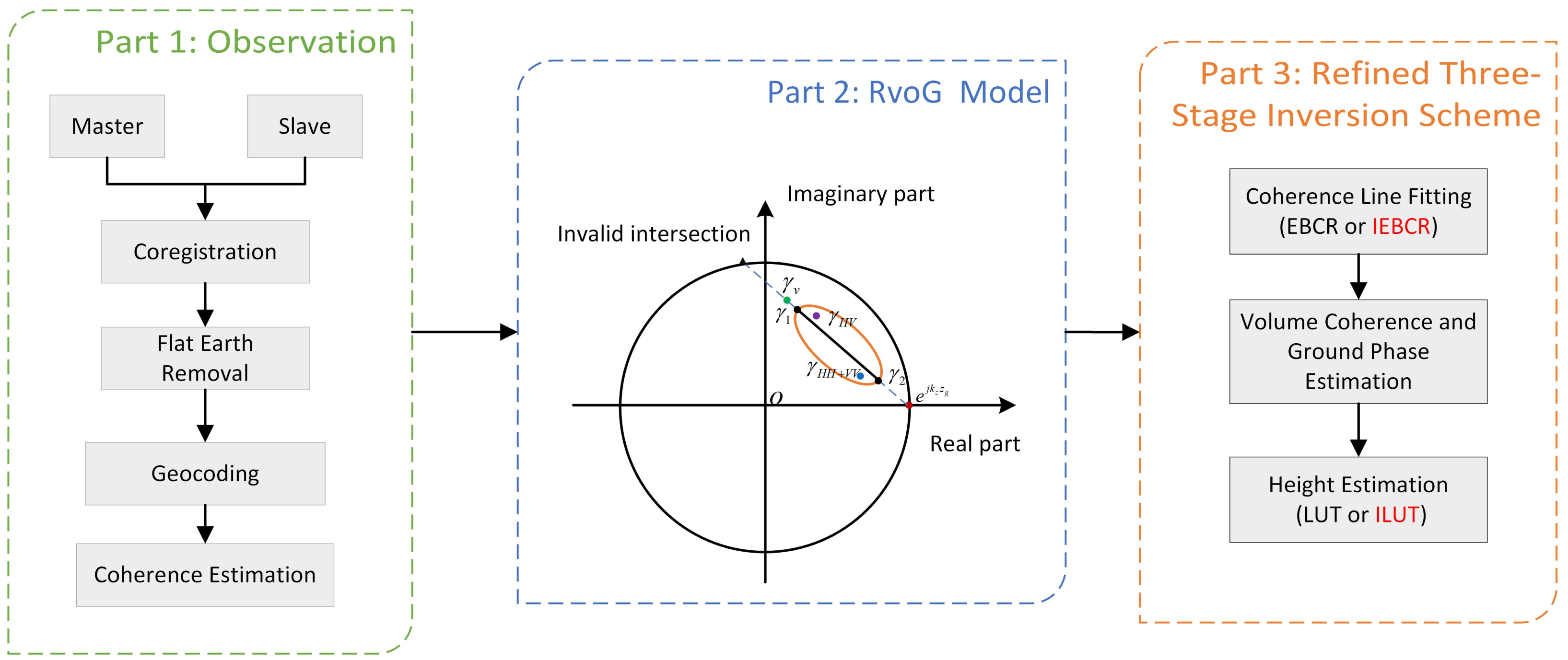
2. Model-Based Pol-InSAR Inversion
2.1. Observation
2.2. RVoG Model
2.3. Refined Three-Stage Inversion Scheme
2.3.1. Coherence Line Fitting
2.3.2. Volume Coherence and Ground Phase Estimation
2.3.3. Height and Extinction Estimation
3. Methods
3.1. IEBCR
| Algorithm 1. IEBCR. |
|
3.2. ILUT
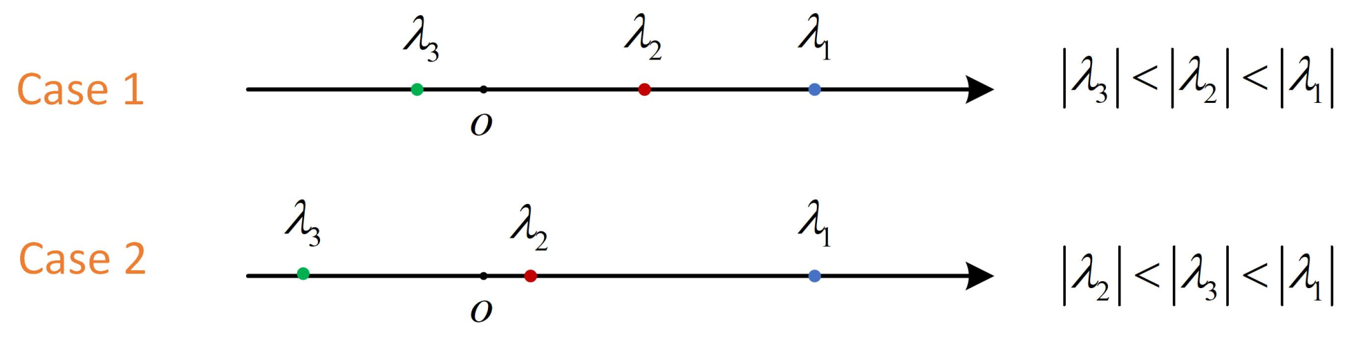
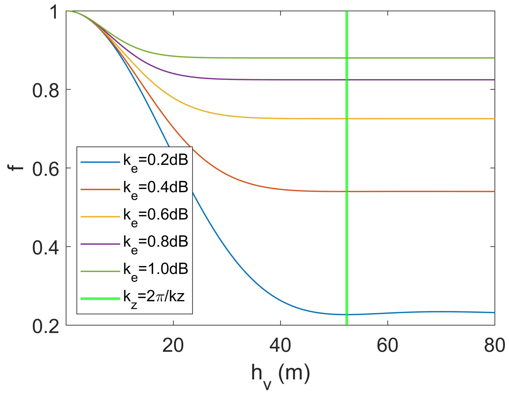
- 1.
- For a fixed , the function converges to a value as the tree height increases. Moreover, the value increases with the increase of .
- 2.
- In the direction of , the function is monotonically decreasing in a specific interval.
- 3.
- In the direction of , the function is monotonically increasing.
3.2.1. Convergence Properties
3.2.2. Monotoncity
3.2.3. ILUT
| Algorithm 2. ILUT. |
|
4. Results
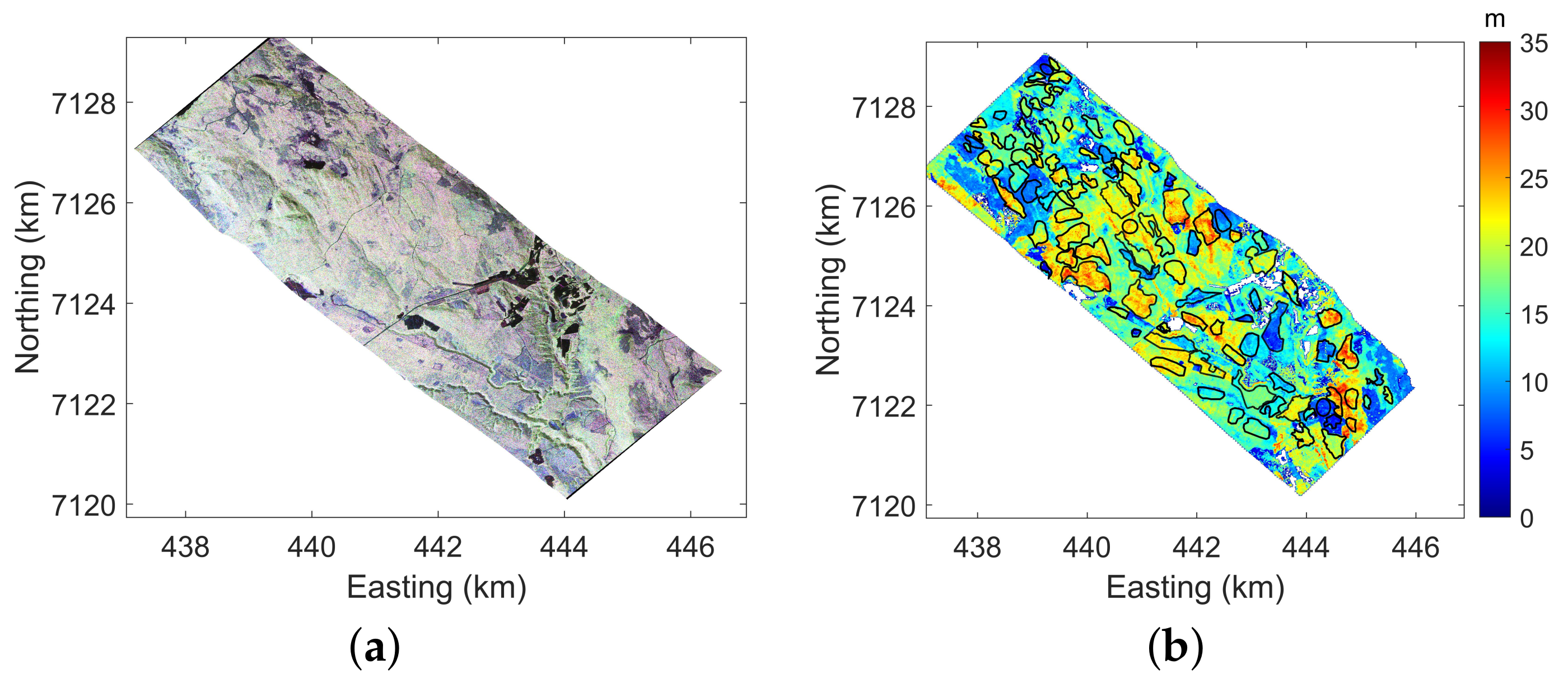
4.1. Data Description
4.2. Evaluation Indicator
4.3. Forest Height Inversion
4.4. Forest Height Validation
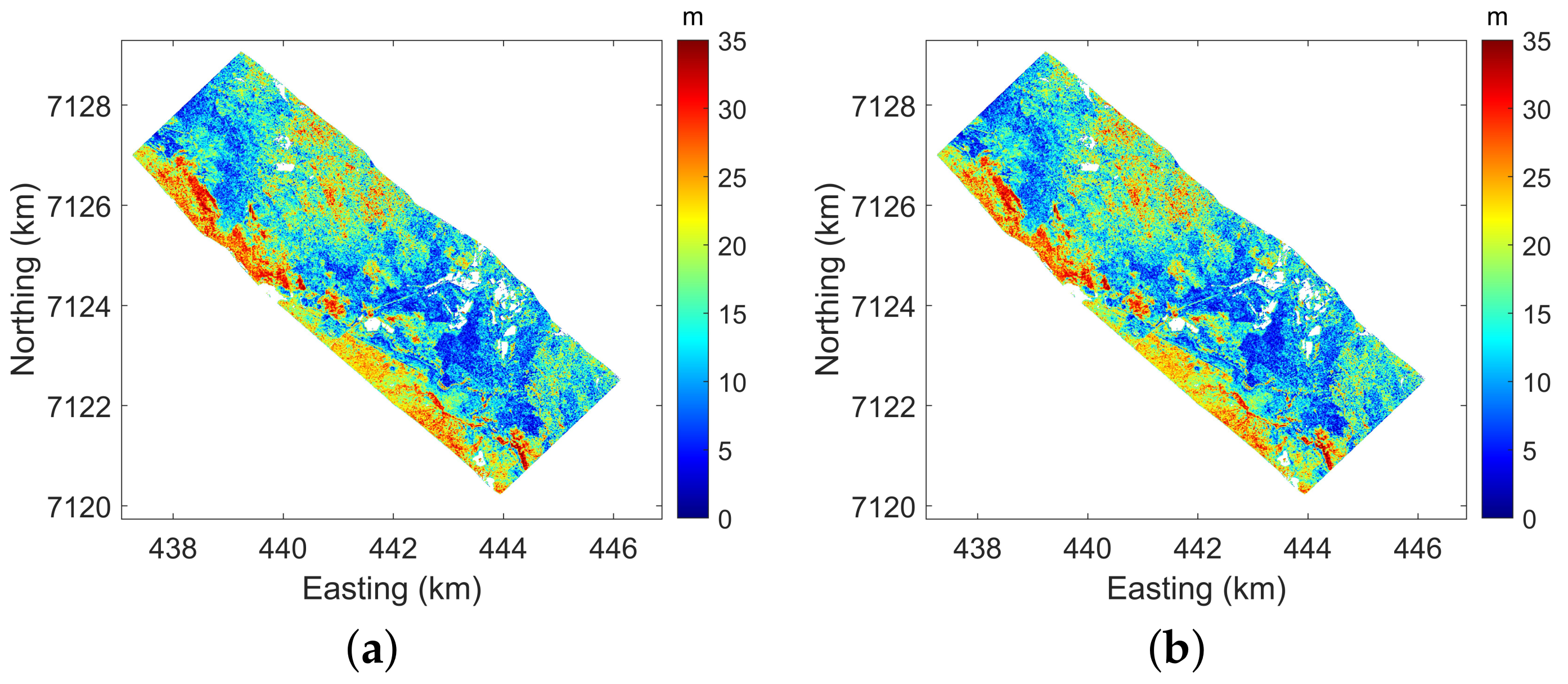
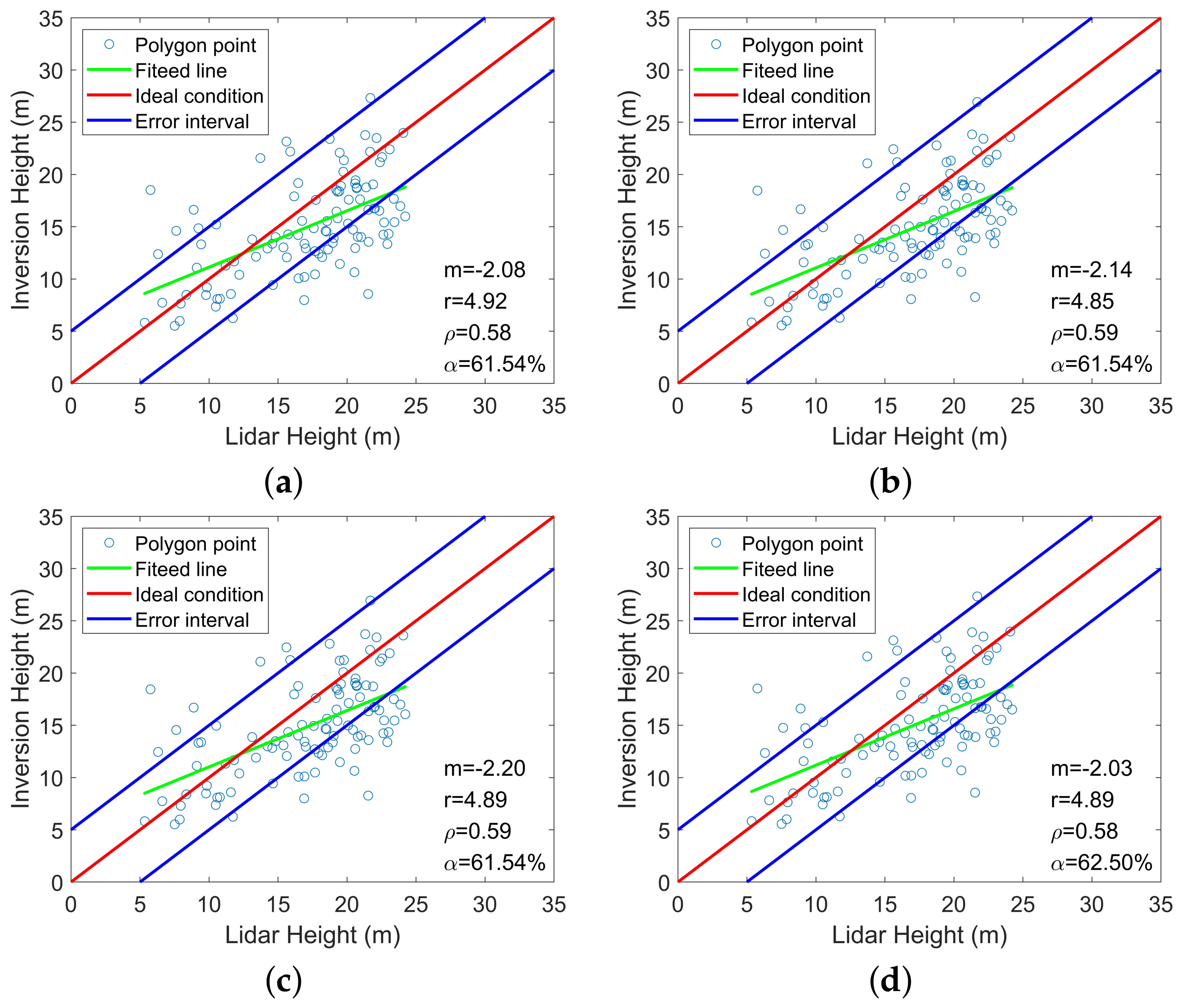
4.4.1. P-Band
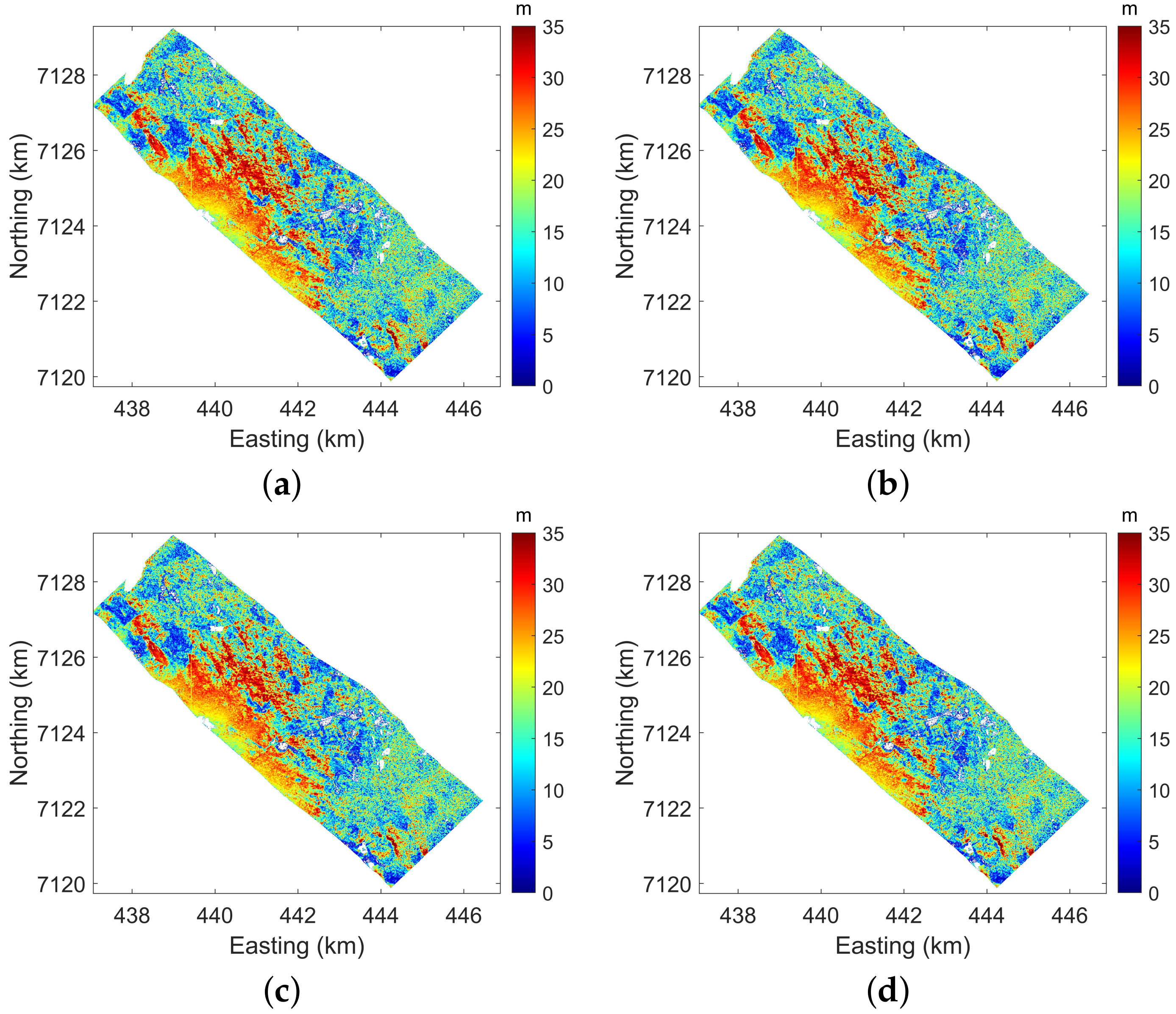
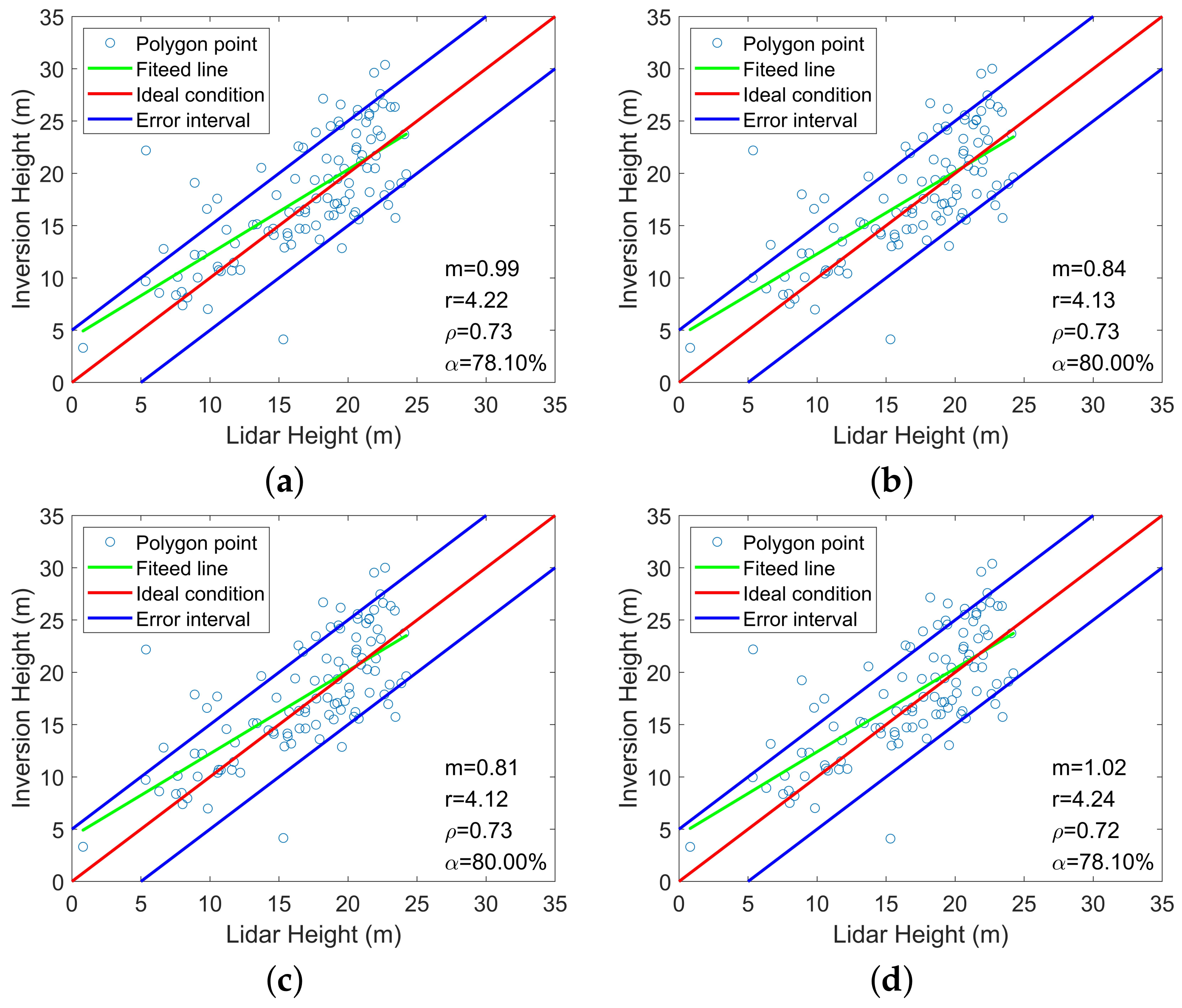
4.4.2. L-Band
5. Discussion
5.1. Quality of Forest Height Estimation
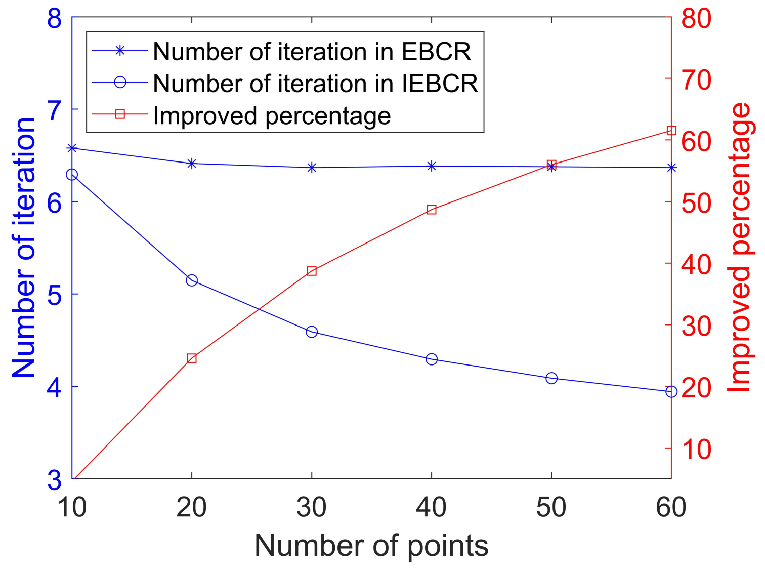
5.2. Analysis of IEBCR
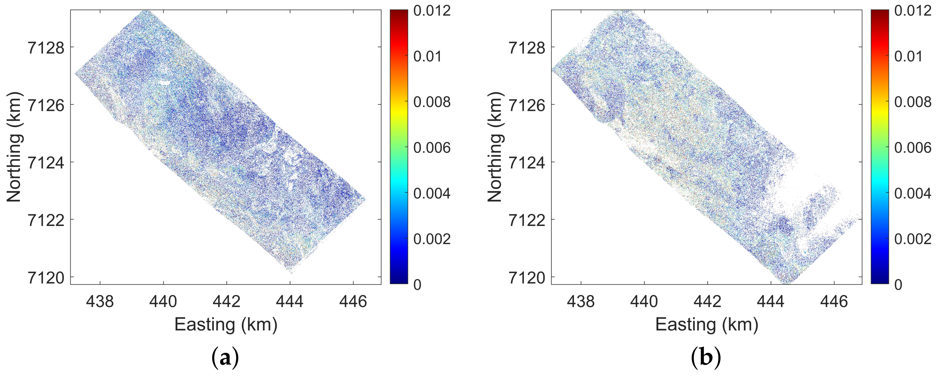
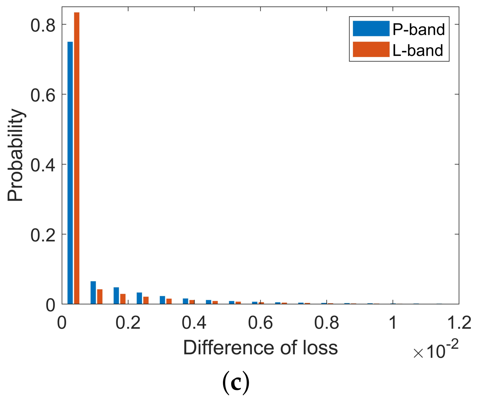
5.2.1. Analysis of the Accuracy
5.2.2. Analysis of Efficiency
5.3. Analysis of ILUT
5.3.1. Analysis of the Accuracy
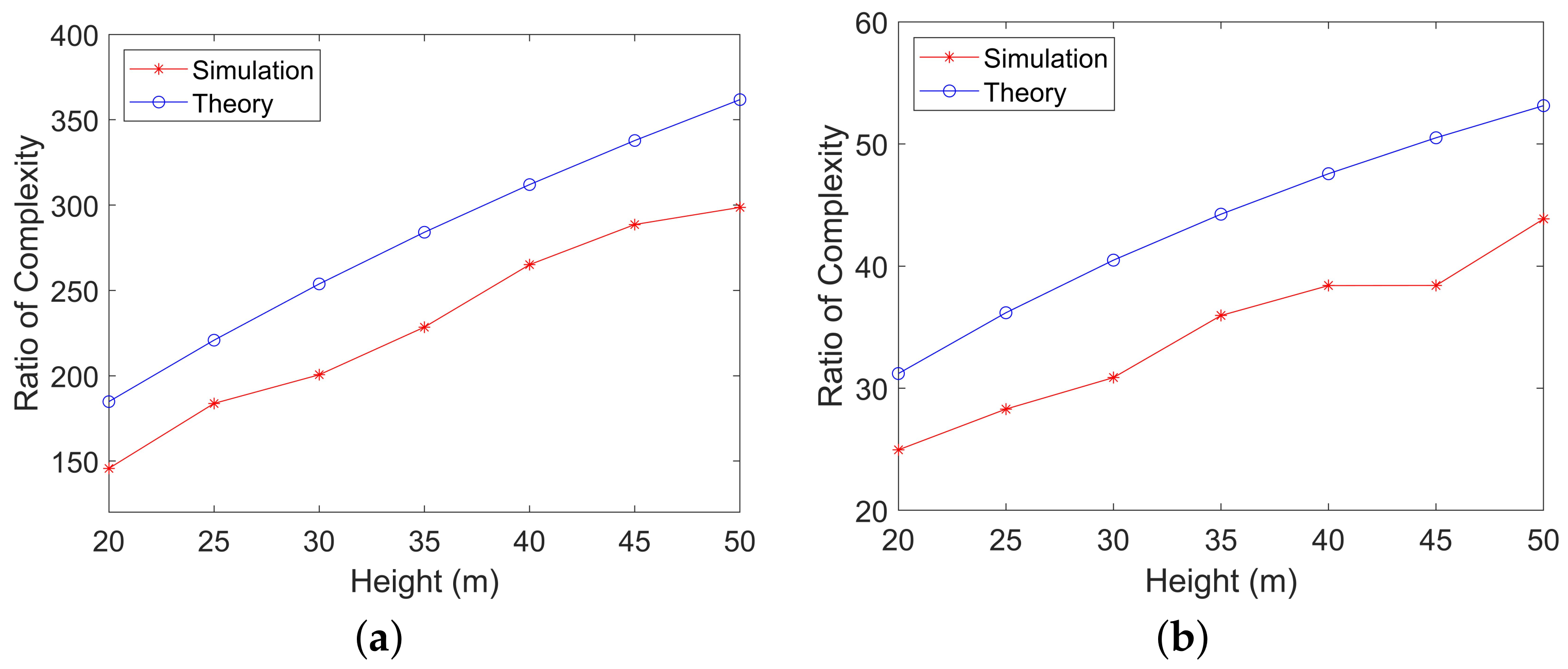
5.3.2. Analysis of the Efficiency
5.4. Limitations of the Proposed Methods
6. Conclusions
- 1.
- The two iterative methods are effective at P- and L-bands in single-baseline forest height inversion.
- 2.
- The iterative methods can significantly improve the computational efficiency without compromising on the accuracy and are applicable to various algorithms for retrieval of forest vertical structure based on the RVoG model.
Author Contributions
Funding
Institutional Review Board Statement
Informed Consent Statement
Data Availability Statement
Acknowledgments
Conflicts of Interest
Abbreviations
| RVoG | Random Volume over Ground |
| TSIA | three-stage inversion algorithm |
| LiDAR | Light Detection And Ranging |
| PolInSAR | Polarimetric Interferometric Synthetic Aperture Radar |
| GVR | ground-to-volume amplitude ratio |
| NGVR | null ground-to-volume amplitude ratio |
| RMoG | Random-Motion-over-Ground |
| VTD | volume temporal decorrelation |
| BCR | boundary of the coherence region |
| EBCR | extraction of the boundary of the coherence region |
| IEBCR | iterative extraction of the boundary of the coherence region |
| LUT | look-up table |
| ILUT | iterative look-up table |
| RMSE | root mean square error |
References
- Toan, T.L.; Villard, L.; Lasne, Y.; Mermoz, S.; Koleck, T. Assessment of tropical forest biomass: A challenging objective for the biomass mission. In Proceedings of the 2012 IEEE International Geoscience and Remote Sensing Symposium, Munich, Germany, 22–27 July 2012; pp. 7581–7584. [Google Scholar] [CrossRef]
- Bergen, K.M.; Goetz, S.J.; Dubayah, R.O.; Henebry, G.M.; Hunsaker, C.T.; Imhoff, M.L.; Nelson, R.F.; Parker, G.G.; Radeloff, V.C. Remote sensing of vegetation 3-D structure for biodiversity and habitat: Review and implications for lidar and radar spaceborne missions. J. Geophys. Res. Biogeosci. 2009, 114, G00E06. [Google Scholar] [CrossRef] [Green Version]
- Le Toan, T.; Quegan, S.; Davidson, M.W.J.; Balzter, H.; Paillou, P.; Papathanassiou, K.; Plummer, S.; Rocca, F.; Saatchi, S.; Shugart, H. The BIOMASS mission: Mapping global forest biomass to better understand the terrestrial carbon cycle. Remote Sens. Environ. 2011, 115, 2850–2860. [Google Scholar] [CrossRef] [Green Version]
- Agata, H.; Aneta, L.; Dariusz, Z.; Krzysztof, S.; Marek, L.; Christiane, S.; Carsten, P. Forest Aboveground Biomass Estimation Using a Combination of Sentinel-1 and Sentinel-2 Data. In Proceedings of the IGARSS 2018—2018 IEEE International Geoscience and Remote Sensing Symposium, Valencia, Spain, 22–27 July 2018; pp. 9026–9029. [Google Scholar] [CrossRef]
- Lefsky, M.A.; Cohen, W.B.; Parker, G.G.; Harding, D.J. Lidar Remote Sensing for Ecosystem Studies: Lidar, an emerging remote sensing technology that directly measures the three-dimensional distribution of plant canopies, can accurately estimate vegetation structural attributes and should be of particular interest to forest, landscape, and global ecologists. BioScience 2002, 52, 19–30. [Google Scholar] [CrossRef]
- Pourshamsi, M.; Xia, J.; Yokoya, N.; Garcia, M.; Lavalle, M.; Pottier, E.; Balzter, H. Tropical forest canopy height estimation from combined polarimetric SAR and LiDAR using machine-learning. ISPRS J. Photogramm. Remote Sens. 2021, 172, 79–94. [Google Scholar] [CrossRef]
- Papathanassiou, K.P.; Cloude, S.R. Single-baseline polarimetric SAR interferometry. IEEE Trans. Geosci. Remote Sens. 2001, 39, 2352–2363. [Google Scholar] [CrossRef] [Green Version]
- Garestier, F.; Dubois-Fernandez, P.C.; Champion, I. Forest height inversion using high-resolution P-band Pol-InSAR data. IEEE Trans. Geosci. Remote Sens. 2008, 46, 3544–3559. [Google Scholar] [CrossRef]
- Soja, M.J.; Persson, H.; Ulander, L.M.H. Estimation of forest height and canopy density from a single InSAR correlation coefficient. IEEE Geosci. Remote Sens. Lett. 2014, 12, 646–650. [Google Scholar] [CrossRef] [Green Version]
- Kugler, F.; Koudogbo, F.; Gutjahr, K.; Papathanassiou, K. Frequency effects in Pol-InSAR forest height estimation. In Proceedings of the European Conference on Synthetic Aperture Radar (EUSAR), Dresden, Germany, 16–18 May 2006; pp. 1–4. [Google Scholar]
- Zhao, L.; Chen, E.; Li, Z.; Zhang, W.; Fan, Y. A New Approach for Forest Height Inversion Using X-Band Single-Pass InSAR Coherence Data. IEEE Trans. Geosci. Remote Sens. 2021, 60, 5206018. [Google Scholar] [CrossRef]
- Sun, X.; Wang, B.; Xiang, M.; Zhou, L.; Jiang, S. Forest Height Estimation Based on P-Band Pol-InSAR Modeling and Multi-Baseline Inversion. Remote Sens. 2020, 12, 1319. [Google Scholar] [CrossRef] [Green Version]
- Soja, M.J.; Persson, H.J.; Ulander, L.M.H. Modeling and Detection of Deforestation and Forest Growth in Multitemporal TanDEM-X Data. IEEE J. Sel. Top. Appl. Earth Obs. Remote Sens. 2018, 11, 3548–3563. [Google Scholar] [CrossRef]
- Kugler, F.; Lee, S.; Hajnsek, I.; Papathanassiou, K.P. Forest Height Estimation by Means of Pol-InSAR Data Inversion: The Role of the Vertical Wavenumber. IEEE Trans. Geosci. Remote Sens. 2015, 53, 5294–5311. [Google Scholar] [CrossRef]
- Wang, X.; Xu, F. A PolinSAR Inversion Error Model on Polarimetric System Parameters for Forest Height Mapping. IEEE Trans. Geosci. Remote Sens. 2019, 57, 5669–5685. [Google Scholar] [CrossRef]
- Chen, H.; Cloude, S.R.; Goodenough, D.G.; Hill, D.A.; Nesdoly, A. Radar Forest Height Estimation in Mountainous Terrain Using Tandem-X Coherence Data. IEEE J. Sel. Top. Appl. Earth Obs. Remote Sens. 2018, 11, 3443–3452. [Google Scholar] [CrossRef]
- Askne, J.I.H.; Santoro, M. On the Estimation of Boreal Forest Biomass From TanDEM-X Data Without Training Samples. IEEE Geosci. Remote Sens. Lett. 2015, 12, 771–775. [Google Scholar] [CrossRef]
- Shi, Y.; He, B.; Liao, Z. An improved dual-baseline PolInSAR method for forest height inversion. Int. J. Appl. Earth Obs. Geoinf. 2021, 103, 102483. [Google Scholar] [CrossRef]
- Parache, H.B.; Mayer, T.; Herndon, K.E.; Flores-Anderson, A.I.; Lei, Y.; Nguyen, Q.; Kunlamai, T.; Griffin, R. Estimating Forest Stand Height in Savannakhet, Lao PDR Using InSAR and Backscatter Methods with L-Band SAR Data. Remote Sens. 2021, 13, 4516. [Google Scholar] [CrossRef]
- Chen, W.; Zheng, Q.; Xiang, H.; Chen, X.; Sakai, T. Forest Canopy Height Estimation Using Polarimetric Interferometric Synthetic Aperture Radar (PolInSAR) Technology Based on Full-Polarized ALOS/PALSAR Data. Remote Sens. 2021, 13, 174. [Google Scholar] [CrossRef]
- Dietterich, T.G. An experimental comparison of three methods for constructing ensembles of decision trees: Bagging, boosting, and randomization. Mach. Learn. 2000, 40, 139–157. [Google Scholar] [CrossRef]
- Smola, A.J.; Schölkopf, B. A tutorial on support vector regression. Stat. Comput. 2004, 14, 199–222. [Google Scholar] [CrossRef] [Green Version]
- Lavalle, M.; Hensley, S. Extraction of Structural and Dynamic Properties of Forests From Polarimetric-Interferometric SAR Data Affected by Temporal Decorrelation. IEEE Trans. Geosci. Remote Sens. 2015, 53, 4752–4767. [Google Scholar] [CrossRef]
- Garestier, F.; Toan, T.L. Forest Modeling For Height Inversion Using Single-Baseline InSAR/Pol-InSAR Data. IEEE Trans. Geosci. Remote Sens. 2010, 48, 1528–1539. [Google Scholar] [CrossRef]
- García, M.; Saatchi, S.; Ustin, S.; Balzter, H. Modelling forest canopy height by integrating airborne LiDAR samples with satellite Radar and multispectral imagery. Int. J. Appl. Earth Obs. Geoinf. 2018, 66, 159–173. [Google Scholar] [CrossRef]
- Brigot, G.; Simard, M.; Colin-Koeniguer, E.; Boulch, A. Retrieval of forest vertical structure from PolInSAR data by machine learning using LIDAR-derived features. Remote Sens. 2019, 11, 381. [Google Scholar] [CrossRef] [Green Version]
- Li, W.; Niu, Z.; Shang, R.; Qin, Y.; Wang, L.; Chen, H. High-resolution mapping of forest canopy height using machine learning by coupling ICESat-2 LiDAR with Sentinel-1, Sentinel-2 and Landsat-8 data. Int. J. Appl. Earth Obs. Geoinf. 2020, 92, 102163. [Google Scholar] [CrossRef]
- Treuhaft, R.N.; Madsen, S.N.; Moghaddam, M.; Zyl, J.J.v. Vegetation characteristics and underlying topography from interferometric radar. Radio Sci. 1996, 31, 1449–1485. [Google Scholar] [CrossRef]
- Treuhaft, R.N.; Siqueira, P.R. Vertical structure of vegetated land surfaces from interferometric and polarimetric radar. Radio Sci. 2000, 35, 141–177. [Google Scholar] [CrossRef] [Green Version]
- Cloude, S.R.; Papathanassiou, K.P. Polarimetric SAR interferometry. IEEE Trans. Geosci. Remote Sens. 1998, 36, 1551–1565. [Google Scholar] [CrossRef]
- Cloude, S.; Papathanassiou, K. Three-stage inversion process for polarimetric SAR interferometry. IEE Proc. Radar Sonar Navig. 2003, 150, 125–134. [Google Scholar] [CrossRef] [Green Version]
- Flynn, T.; Tabb, M.; Carande, R. Coherence region shape extraction for vegetation parameter estimation in polarimetric SAR interferometry. In Proceedings of the IEEE International Geoscience and Remote Sensing Symposium, Toronto, ON, Canada, 24–28 June 2002; Volume 5, pp. 2596–2598. [Google Scholar] [CrossRef]
- Mark, T.; Jeffrey, O.; Thomas, F.; Richard, C. Phase diversity: A decomposition for vegetation parameter estimation using polarimetric SAR interferometry. In Proceedings of the European Conference on Synthetic Aperture Radar EUSAR, Koln, Germany, 4–6 June 2002; pp. 721–724. [Google Scholar]
- Lavalle, M. Full and Compact Polarimetric Radar Interferometry for Vegetation Remote Sensing. Ph.D. Thesis, Université Rennes 1, Rennes, France, 2009. [Google Scholar]
- Colin, E.; Titin-Schnaider, C.; Tabbara, W. An interferometric coherence optimization method in radar polarimetry for high-resolution imagery. IEEE Trans. Geosci. Remote Sens. 2006, 44, 167–175. [Google Scholar] [CrossRef]
- Lu, H.X.; Song, W.Q.; Li, F.; Wang, Y.H.; Liu, H.W.; Bao, Z.; Huang, H.F. Forest parameters inversion based on nonstationarity compensation and mapping space regularization. J. Electron. Inf. Technol. 2015, 37, 283–290. [Google Scholar]
- Liao, Z.; He, B.; Bai, X.; Quan, X. Improving forest height retrieval by reducing the ambiguity of volume-only coherence using multi-baseline PolInSAR data. IEEE Trans. Geosci. Remote Sens. 2019, 57, 8853–8866. [Google Scholar] [CrossRef]
- Touzi, R.; Lopes, A.; Bruniquel, J.; Vachon, P. Coherence estimation for SAR imagery. IEEE Trans. Geosci. Remote. Sens. 1999, 37, 135–149. [Google Scholar] [CrossRef] [Green Version]
- Wold, S.; Esbensen, K.; Geladi, P. Principal component analysis. Chemom. Intell. Lab. Syst. 1987, 2, 37–52. [Google Scholar] [CrossRef]
- Neumann, M.; Reigber, A.; Ferro-Famil, L. Data classification based on PolInSAR coherence shapes. In Proceedings of the 2005 IEEE International Geoscience and Remote Sensing Symposium, Seoul, Korea, 29 July 2005; Volume 7, pp. 4852–4855. [Google Scholar] [CrossRef]
- Mathias, R. Matrices with positive definite Hermitian part: Inequalities and linear systems. SIAM J. Matrix Anal. Appl. 1992, 13, 640–654. [Google Scholar] [CrossRef] [Green Version]
- Al-Hawari, M. Hermitian Part, and Skew Hermitian Part of Normal Matrices; Istanbul Commerce University: Istanbul, Turkey, 2016; p. 23. [Google Scholar]
- Andrilli, S.; Hecker, D. Numerical methods. In Elementary Linear Algebra, 4th ed.; Andrilli, S., Hecker, D., Eds.; Academic Press: Boston, MA, USA, 2010; Chapter 9; pp. 587–643. [Google Scholar] [CrossRef]
- Horn, R.A.; Johnson, C.R. Matrix Analysis; Cambridge University Press: Cambridge, UK, 2012. [Google Scholar]
- Irena, H.; Rolf, S.; Martin, K.; Ralf, H.; Seungkuk, L.; Lars, U.; Anders, G.; Gustaf, S.; Thuy, L.T.; Stefano, T.; et al. BioSAR 2008 Experiment Final Report. Report. 2009. Available online: https://earth.esa.int/eogateway/documents/20142/37627/BIOSAR2_final_report.pdf (accessed on 5 May 2022).
- Laudon, H.; Hasselquist, E.M.; Peichl, M.; Lindgren, K.; Sponseller, R.; Lidman, F.; Kuglerova, L.; Hasselquist, N.J.; Bishop, K.; Nilsson, M.B.; et al. Northern landscapes in transition: Evidence, approach and ways forward using the Krycklan Catchment Study. Hydrol. Process. 2021, 35, e14170. [Google Scholar] [CrossRef]
- Hajnsek, I.; Kugler, F.; Lee, S.; Papathanassiou, K.P. Tropical-Forest-Parameter Estimation by Means of Pol-InSAR: The INDREX-II Campaign. IEEE Trans. Geosci. Remote Sens. 2009, 47, 481–493. [Google Scholar] [CrossRef] [Green Version]
- Keys, R. Cubic convolution interpolation for digital image processing. IEEE Trans. Acoust. Speech Signal Process. 1981, 29, 1153–1160. [Google Scholar] [CrossRef] [Green Version]


| Band | L | P |
|---|---|---|
| Centre Frequency | 1.300 GHz | 0.349 GHz |
| Spatial Baseline | 6, 12, 18, 24, 30 m | 8, 16, 24, 32, 40 m |
| Flight Direction | and | |
| Easting size | 9561 | |
| Northing size | 9821 | |
| Easting Range | 437,061–446,881 m | |
| Northing Range | 7,119,733–7,129,293 m | |
| Geocoded Resolution | 1 m × 1 m | |
Publisher’s Note: MDPI stays neutral with regard to jurisdictional claims in published maps and institutional affiliations. |
© 2022 by the authors. Licensee MDPI, Basel, Switzerland. This article is an open access article distributed under the terms and conditions of the Creative Commons Attribution (CC BY) license (https://creativecommons.org/licenses/by/4.0/).
Share and Cite
Huang, Z.; Yun, Y.; Chai, H.; Lv, X. The Iterative Extraction of the Boundary of Coherence Region and Iterative Look-Up Table for Forest Height Estimation Using Polarimetric Interferometric Synthetic Aperture Radar Data. Remote Sens. 2022, 14, 2438. https://0-doi-org.brum.beds.ac.uk/10.3390/rs14102438
Huang Z, Yun Y, Chai H, Lv X. The Iterative Extraction of the Boundary of Coherence Region and Iterative Look-Up Table for Forest Height Estimation Using Polarimetric Interferometric Synthetic Aperture Radar Data. Remote Sensing. 2022; 14(10):2438. https://0-doi-org.brum.beds.ac.uk/10.3390/rs14102438
Chicago/Turabian StyleHuang, Zenghui, Ye Yun, Huiming Chai, and Xiaolei Lv. 2022. "The Iterative Extraction of the Boundary of Coherence Region and Iterative Look-Up Table for Forest Height Estimation Using Polarimetric Interferometric Synthetic Aperture Radar Data" Remote Sensing 14, no. 10: 2438. https://0-doi-org.brum.beds.ac.uk/10.3390/rs14102438